Embed Size (px)
Citation preview
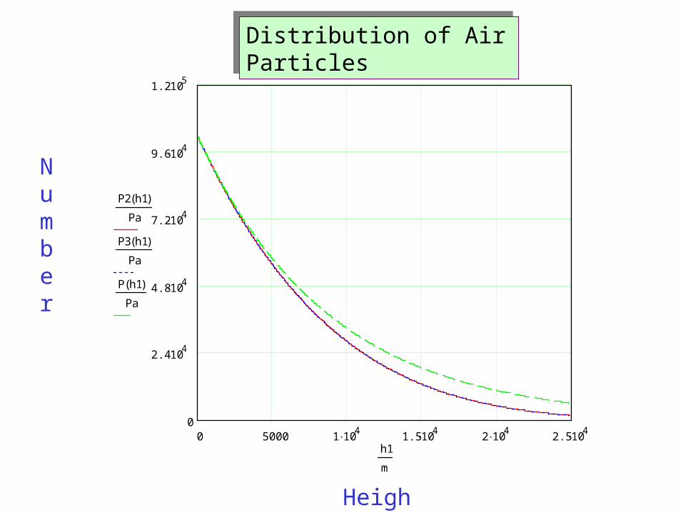
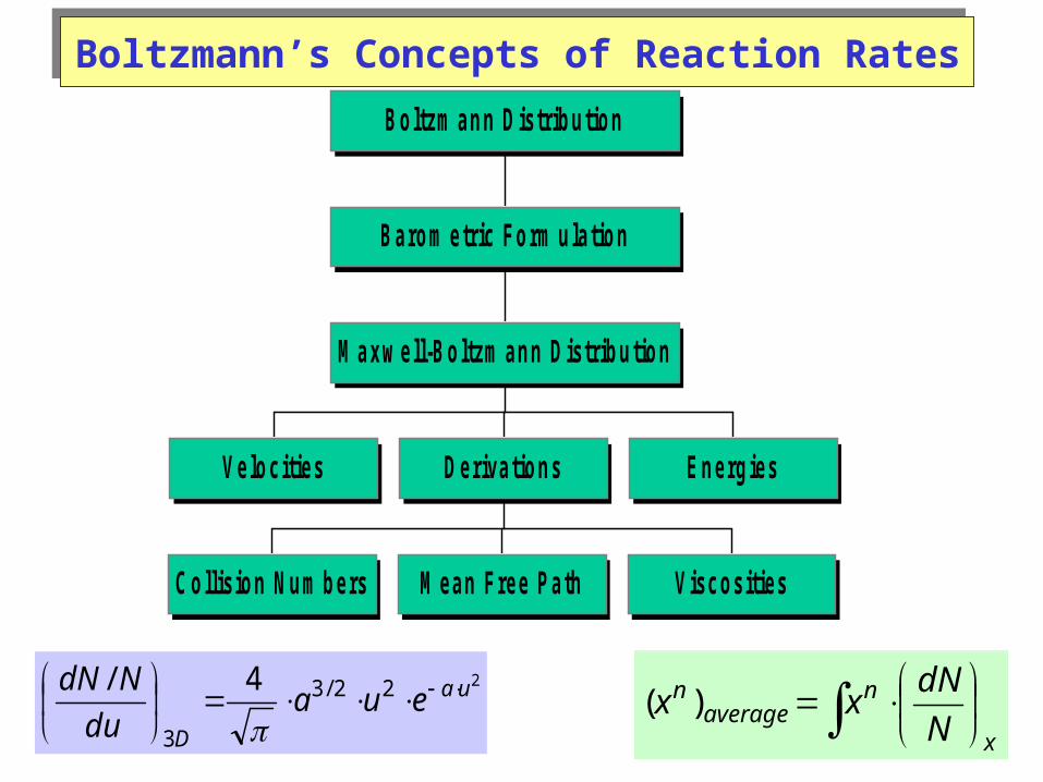
Boltzmann’s Concepts of Reaction RatesBoltzmann’s Concepts of Reaction Rates
Velocities
Collision Num bers M ean Free Path Viscosities
Derivations Energies
M axw ell-Boltzm ann Distribution
Barom etric Form ulation
Boltzm ann Distribution
04/18/23
0 5000 1 104
1.5 104
2 104
2.5 104
0
2.4 104
4.8 104
7.2 104
9.6 104
1.2 105
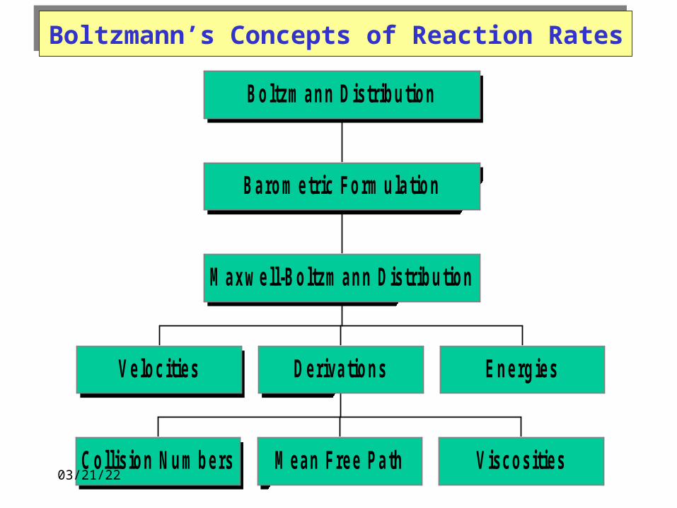
P2 h1( )
Pa
P3 h1( )
Pa
P h1( )
Pa
h1
m
Distribution of Air ParticlesDistribution of Air Particles
Number
Height

Distribution of Molecular Energy LevelsDistribution of Molecular Energy Levels
EquationBoltzmanneg
g
N
N kTE
j
i
j
i /
Where: E = Ei – Ej & e-E/kT = Boltzman Factor
If Boltz. Factor Comment
E << kT Close to 1 Ratio of population is equal
E ~ kT 1/e = 0.368 Upper level drops suddenly
E >> kT About 0 Zero upper level population

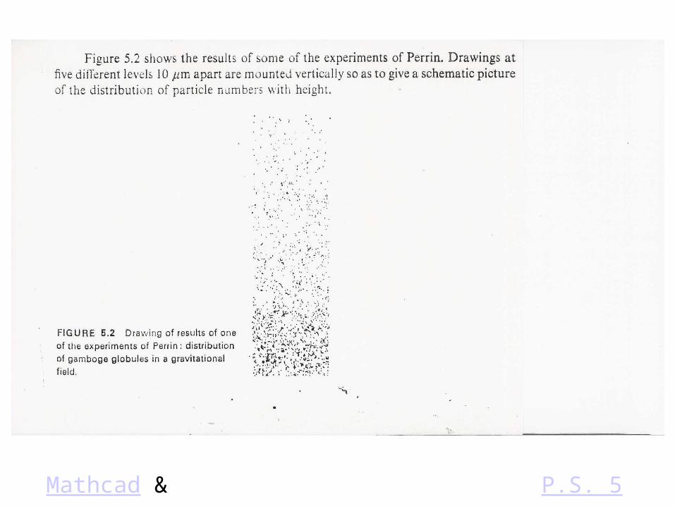
(S14) The Barometric Formulation(S14) The Barometric Formulation
(S14) The Barometric Formulation(S14) The Barometric Formulation
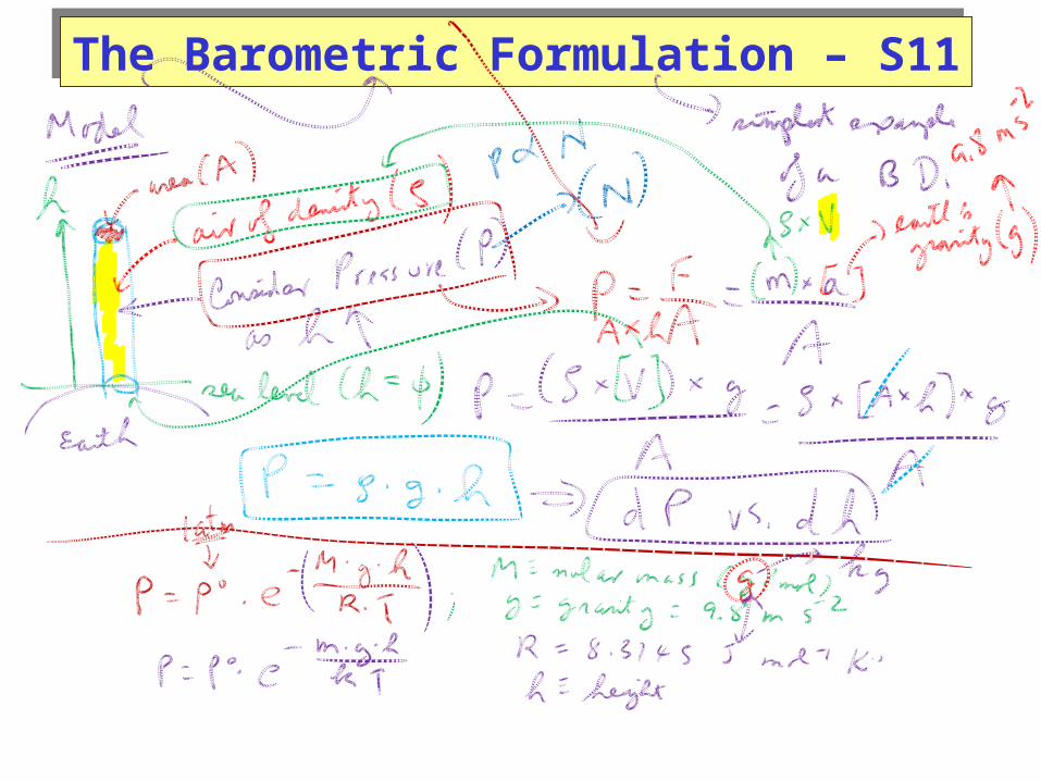
The Barometric Formulation – S11The Barometric Formulation – S11

The Barometric FormulationThe Barometric Formulation
• Calculate the pressure at mile high city (Denver, CO). [1 mile = 1610 m] Po = 101.325 kPa , T = 300. K . Assume 20.0 and 80.0 mole % of oxygen gas and nitrogen gas, respectively.

Molecular TemperatureMolecular Temperature
Distribution Measurement of
VibrationalTemp. in Hot Gases, Plasmas, Explosions
RotationalLow Temp. in Interstellar Gases
ElectronicHigh Stellar Temp. of Atoms and Ions

The Kinetic Molecular Model for Gases ( Postulates )
The Kinetic Molecular Model for Gases ( Postulates )
• Gas consists of large number of small individual particles with negligible size
• Particles in constant random motion and collisions
• No forces exerted among each other
• Kinetic energy directly proportional to temperature in Kelvin
TRKE 2
3
K-M Model: Root-Mean-Square SpeedK-M Model: Root-Mean-Square Speed

Maxwell-Boltzmann DistributionMaxwell-Boltzmann Distribution
M-B Equation gives distribution of molecules in terms of:
•Speed/Velocity, and
•Energy
One-dimensional Velocity Distribution in the x-direction:
[ 1Du-x ]
x
TkumdueA
N
dN x
/2
1 2

1500 1000 500 0 500 1000 15000
5 104
0.001
0.0015
0.002
0.0025
0
F1 u( )
m1
s
F2 u( )
m1
s
F3 u( )
m1
s
15001500 u
m s1
x
TkumdueA
N
dN x
/2
1 2
Mcad
MB Distribution: NormalizationMB Distribution: Normalization
Integral Tables

1D-x Maxwell-Boltzmann Distribution1D-x Maxwell-Boltzmann Distribution
One-dimensional Velocity Distribution in the x-direction: [ 1Du-x ]
x
Tkum
uD
dueTk
m
N
dN x
x
/2
1
1
2
2
One-dimensional Energy Distribution in the x-direction: [ 1DE-x ]
xTk
xED
deTkN
dNx
x
/2
1
1 4
1

x
Tkum
uD
dueTk
m
N
dN x
x
/2
1
1
2
2
xTk
xED
deTkN
dNx
x
/2
1
1 4
1
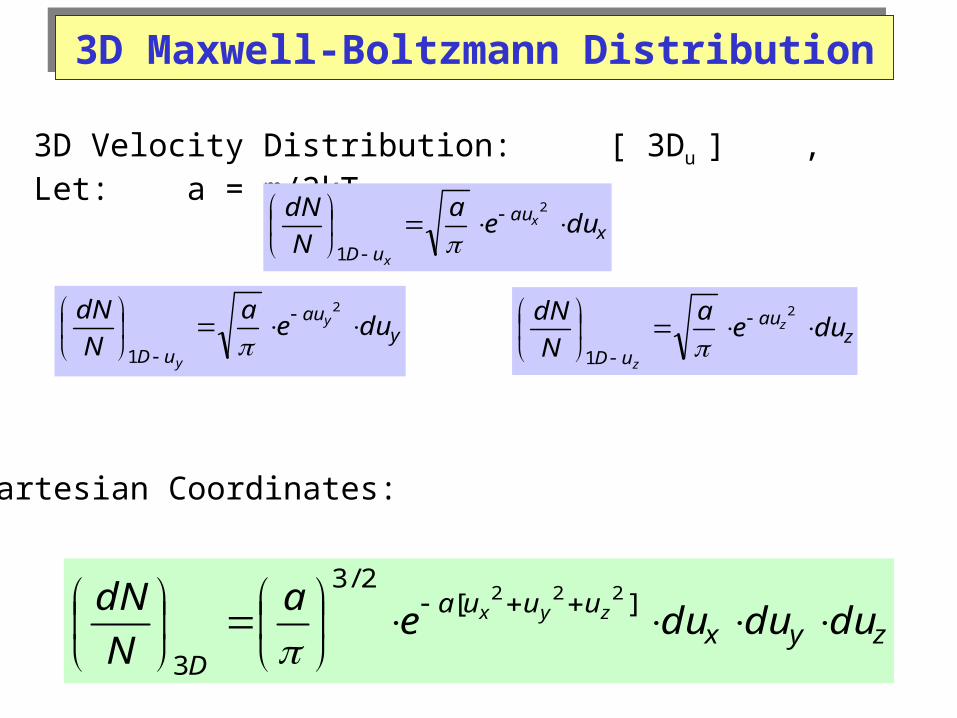
3D Maxwell-Boltzmann Distribution3D Maxwell-Boltzmann Distribution
3D Velocity Distribution: [ 3Du ] , Let: a = m/2kT
xau
uD
duea
N
dNx
x
2
1
Cartesian Coordinates:
zyxuuua
D
dududuea
N
dN zyx
][
2/3
3
222
yau
uD
duea
N
dN y
y
2
1 zau
uD
duea
N
dNz
z
2
1
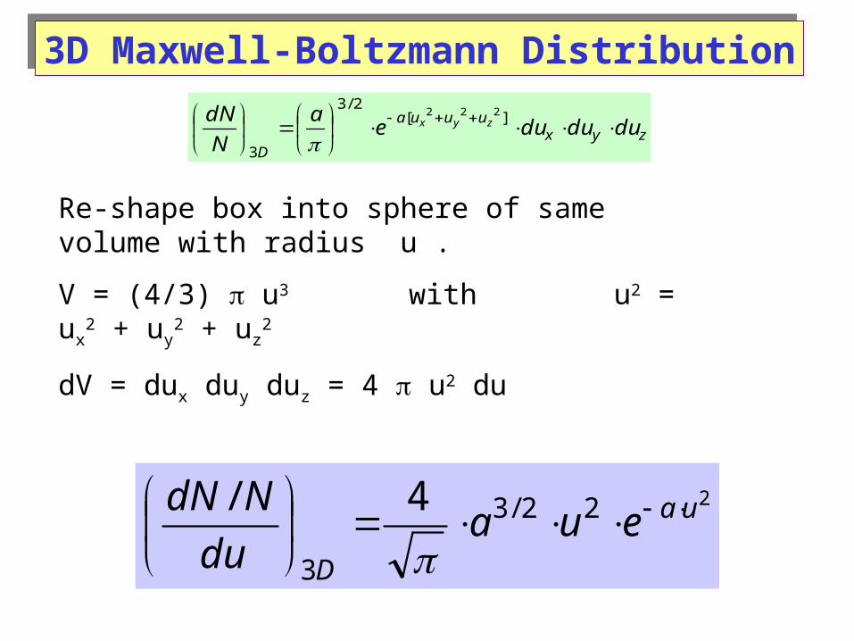
3D Maxwell-Boltzmann Distribution3D Maxwell-Boltzmann Distribution
Re-shape box into sphere of same volume with radius u .
V = (4/3) u3 with u2 = ux2 + uy
2 + uz2
dV = dux duy duz = 4 u2 du
222/3
3
4/ ua
D
euadu
NdN
zyxuuua
D
dududuea
N
dN zyx
][
2/3
3
222

0 500 1000 1500 2000 25000
0.001
0.002
0.003
0.0035
0
F1 u( )
m1
s
F2 u( )
m1
s
F3 u( )
m1
s
25000 u
m s1
3D Maxwell-Boltzmann Distribution3D Maxwell-Boltzmann Distribution
Low T
High T
Mcad


3D Maxwell-Boltzmann Distribution3D Maxwell-Boltzmann Distribution
Conversion of Velocity-distribution to Energy-distribution:
= ½ m u2 ; d = mu du
222/3
3
4/ ua
uD
euadu
NdN
kT
D
ekTd
NdN
2/1
2/3
3
12/
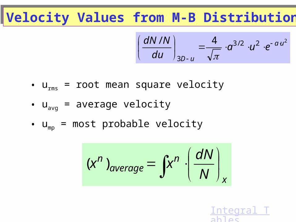
Velocity Values from M-B DistributionVelocity Values from M-B Distribution
• urms = root mean square velocity
• uavg = average velocity
• ump = most probable velocity
x
naverage
n
N
dNxx )(
222/3
3
4/ ua
uD
euadu
NdN
Integral Tables

Velocity Value from M-B Distribution – S14Velocity Value from M-B Distribution – S14
Integral Tables
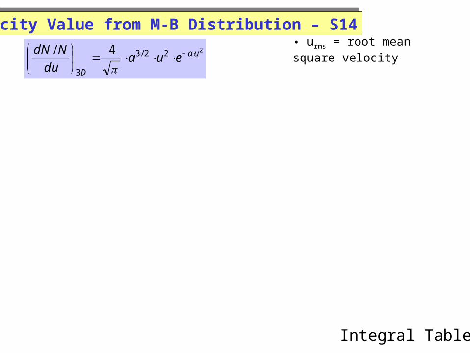
Velocity Value from M-B Distribution – S14Velocity Value from M-B Distribution – S14• urms = root mean square velocity
222/3
3
4/ ua
D
euadu
NdN
Integral Tables
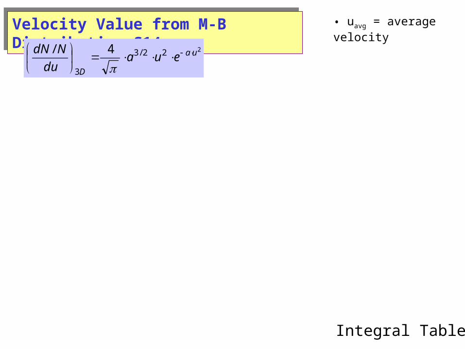
Velocity Value from M-B Distribution S14Velocity Value from M-B Distribution S14 • uavg = average velocity
222/3
3
4/ ua
D
euadu
NdN
Integral Tables

Velocity Value from M-B Distribution S14Velocity Value from M-B Distribution S14 • ump = most probable velocity
222/3
3
4/ ua
D
euadu
NdN
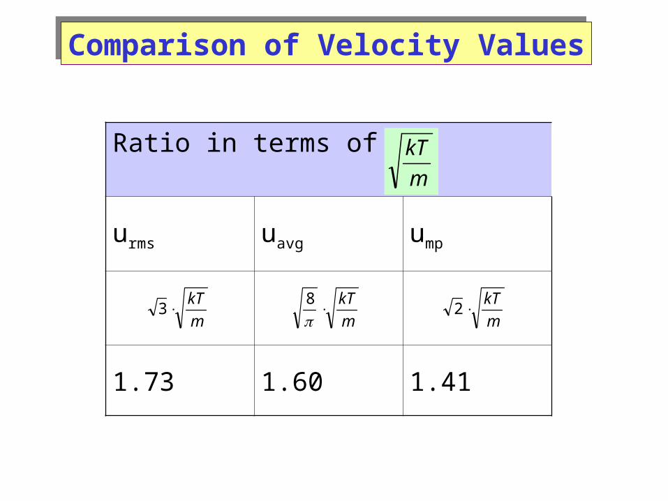
Comparison of Velocity ValuesComparison of Velocity Values
Ratio in terms of :
urms uavg ump
1.73 1.60 1.41
m
kT
m
kT3
m
kT
8
m
kT2
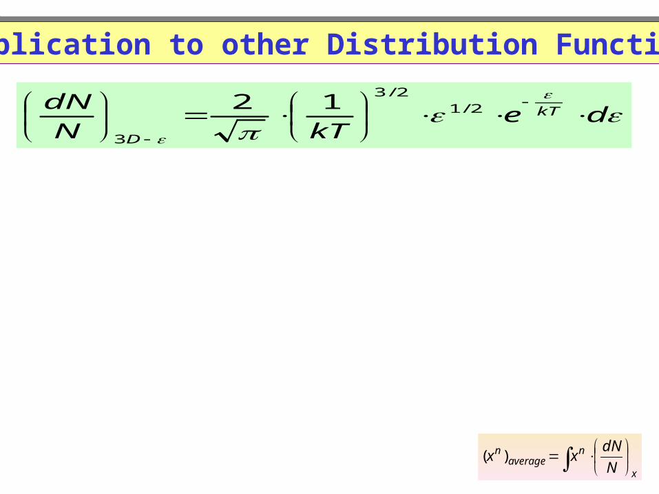
Application to other Distribution FunctionsApplication to other Distribution Functions
de
kTN
dN kT
D
2/12/3
3
12
x
naverage
n
N
dNxx )(
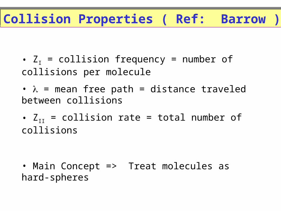
Collision Properties ( Ref: Barrow )Collision Properties ( Ref: Barrow )
• ZI = collision frequency = number of collisions per molecule
• = mean free path = distance traveled between collisions
• ZII = collision rate = total number of collisions
• Main Concept => Treat molecules as hard-spheres
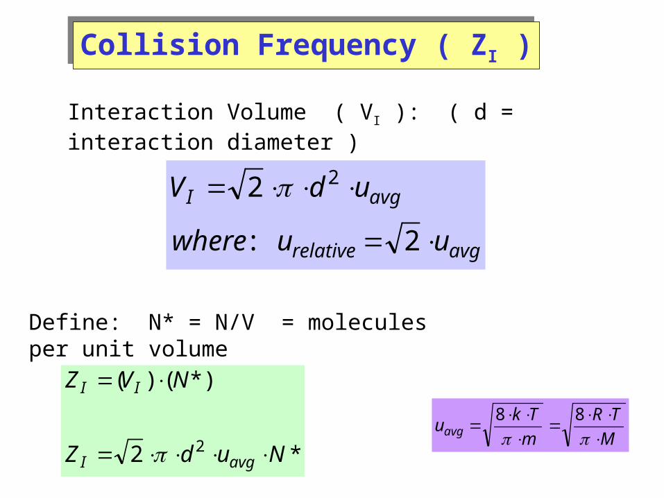
Collision Frequency ( ZI )Collision Frequency ( ZI )
Interaction Volume ( VI ): ( d = interaction diameter )
avgrelative
avgI
uuwhere
udV
2:
2 2
Define: N* = N/V = molecules per unit volume
*2
*)()(
2 NudZ
NVZ
avgI
II
M
TR
m
Tkuavg
88
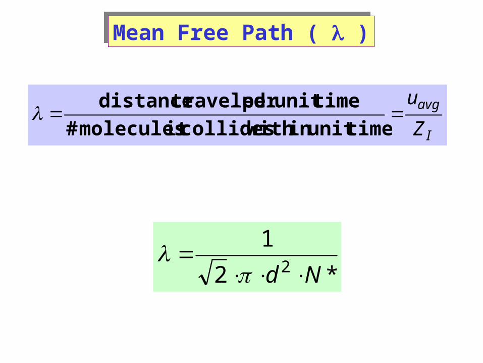
Mean Free Path ( )Mean Free Path ( )
I
avg
Z
u
timeunit in with collidesit molecules #
timeunit per traveled distance
*2
12 Nd
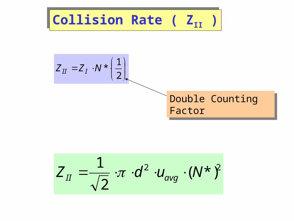
Collision Rate ( ZII )Collision Rate ( ZII )
2
1*NZZ III
Double Counting FactorDouble Counting Factor
22 *)(2
1NudZ avgII
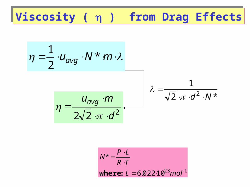
Viscosity ( ) from Drag EffectsViscosity ( ) from Drag Effects
mNuavg *2
1
*2
12 Nd
222 d
muavg
12310022.6
*
molL
TR
LPN
:where

Kinetic-Molecular-Theory Gas Properties - Collision Parameters @ 25oC and 1 atm
Species
Collision diameterMean free path
Collision Frequency
Collision Rate
d / 10-10 m d / Å / 10-8 m ZI / 109 s-1 ZII / 1034 m-3 s-1
H2 2.73 2.73 12.4 14.3 17.6
He 2.18 2.18 19.1 6.6 8.1N2 3.74 3.74 6.56 7.2 8.9O2 3.57 3.57 7.16 6.2 7.6
Ar 3.62 3.62 6.99 5.7 7.0CO2 4.56 4.56 4.41 8.6 10.6
HI 5.56 5.56 2.96 7.5 10.6

Boltzmann’s Concepts of Reaction RatesBoltzmann’s Concepts of Reaction Rates
Velocities
Collision Num bers M ean Free Path Viscosities
Derivations Energies
M axw ell-Boltzm ann Distribution
Barom etric Form ulation
Boltzm ann Distribution
222/3
3
4/ ua
D
euadu
NdN
x
naverage
n
N
dNxx )(
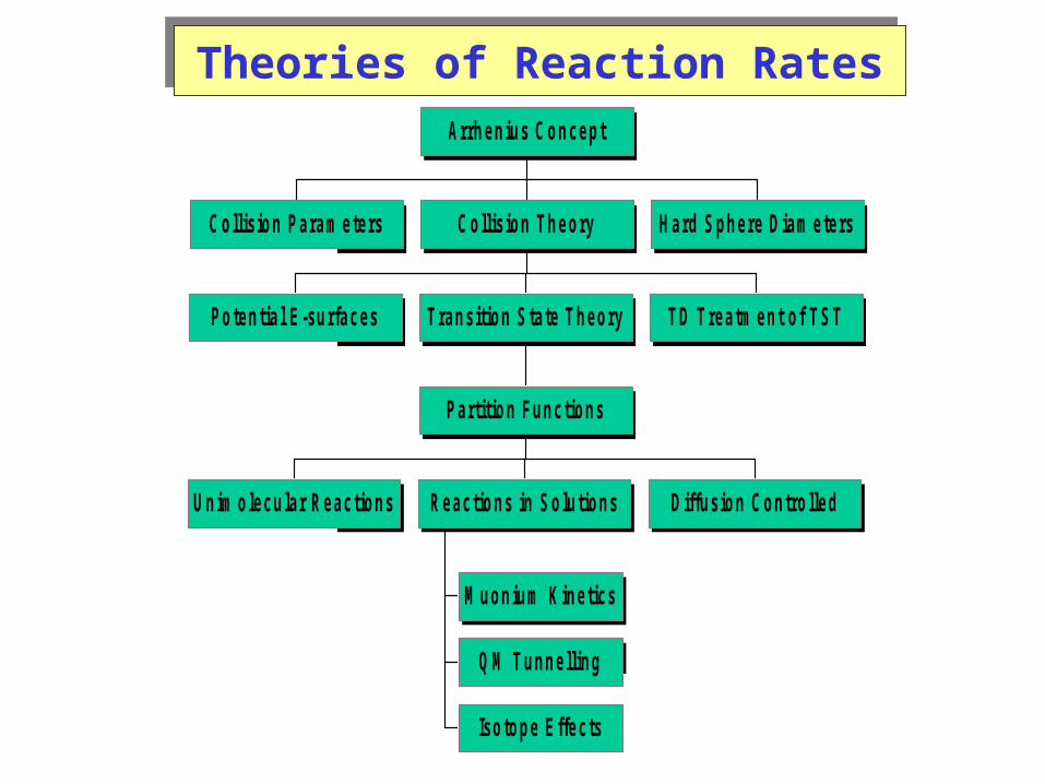
Theories of Reaction RatesTheories of Reaction Rates
Collision Param eters
Potential E -surfaces
Unim olecular Reactions
M uonium Kinetics
QM T unnelling
Isotope Effects
Reactions in Solutions Diffusion Controlled
Partition Functions
T ransition State T heory T D T reatm ent of T ST
Collision T heory Hard Sphere Diam eters
Arrhenius Concept

The Arrhenius Equation• Arrhenius discovered most reaction-rate data obeyed the
Arrhenius equation:
• Including natural phenomena such as:• Chirp rates of crickets• Creeping rates of ants
Arrhenius ConceptArrhenius Concept
TR
Ea
eAk
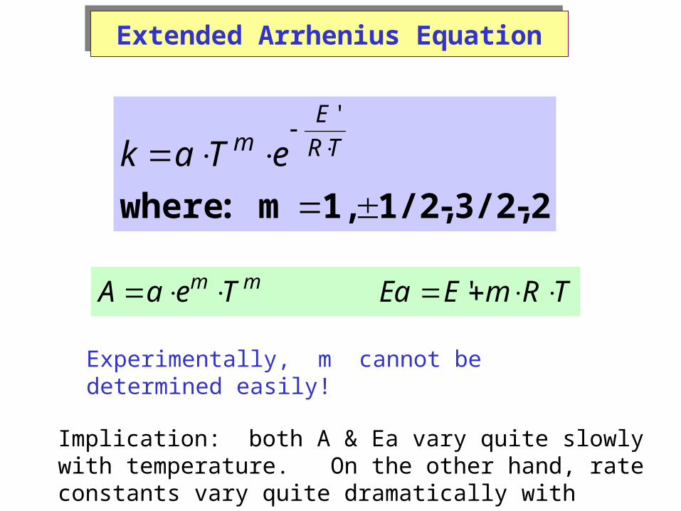
Extended Arrhenius EquationExtended Arrhenius Equation
2- 3/2,- 1/2, 1,m :where
TR
Em eTak
'
Experimentally, m cannot be determined easily!
TRmEEaTeaA mm '
Implication: both A & Ea vary quite slowly with temperature. On the other hand, rate constants vary quite dramatically with temperature,
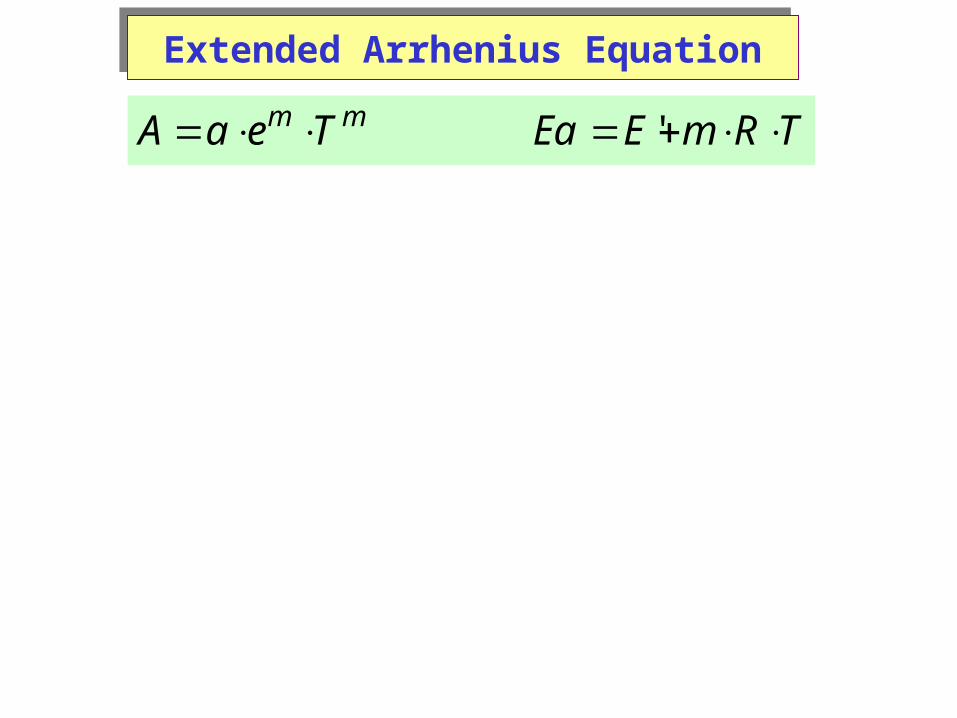
Extended Arrhenius EquationExtended Arrhenius Equation
TRmEEaTeaA mm '
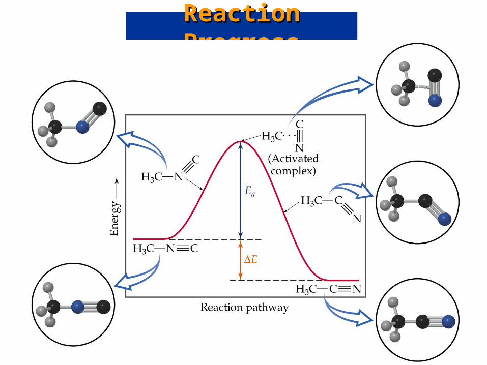
Reaction ProgressReaction Progress

Collision TheoryCollision Theory
Main Concept: Rate Determining Step requires Bimolecular Encounter (i.e. collision)
Rxn Rate = (Collision Rate Factor) x (Activation Energy)
ZII (from simple hard sphere collision properties)
ZII (from simple hard sphere collision properties)
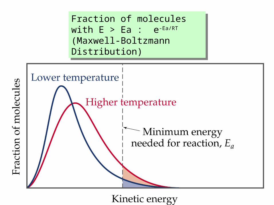
Fraction of molecules with E > Ea : e-Ea/RT (Maxwell-Boltzmann Distribution)
Fraction of molecules with E > Ea : e-Ea/RT (Maxwell-Boltzmann Distribution)
Fraction of molecules with E > Ea : e-Ea/RT (Maxwell-Boltzmann Distribution)
Fraction of molecules with E > Ea : e-Ea/RT (Maxwell-Boltzmann Distribution)

Collision Theory: collision rate ( ZII )Collision Theory: collision rate ( ZII )
][*)(2
1 22avgII vvvdNZ
M
TR
m
Tkv
88
For A-B collisions: AB , vAB
ABAB
BA
BAAB
Tkv
mm
mm
8Velocity Relative
Mass Reduced
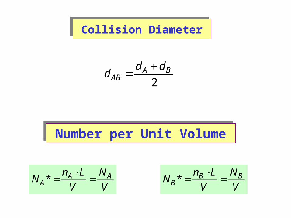
Collision DiameterCollision Diameter
2BA
ABdd
d
Number per Unit VolumeNumber per Unit Volume
V
N
V
LnN AA
A
*V
N
V
LnN BBB
*
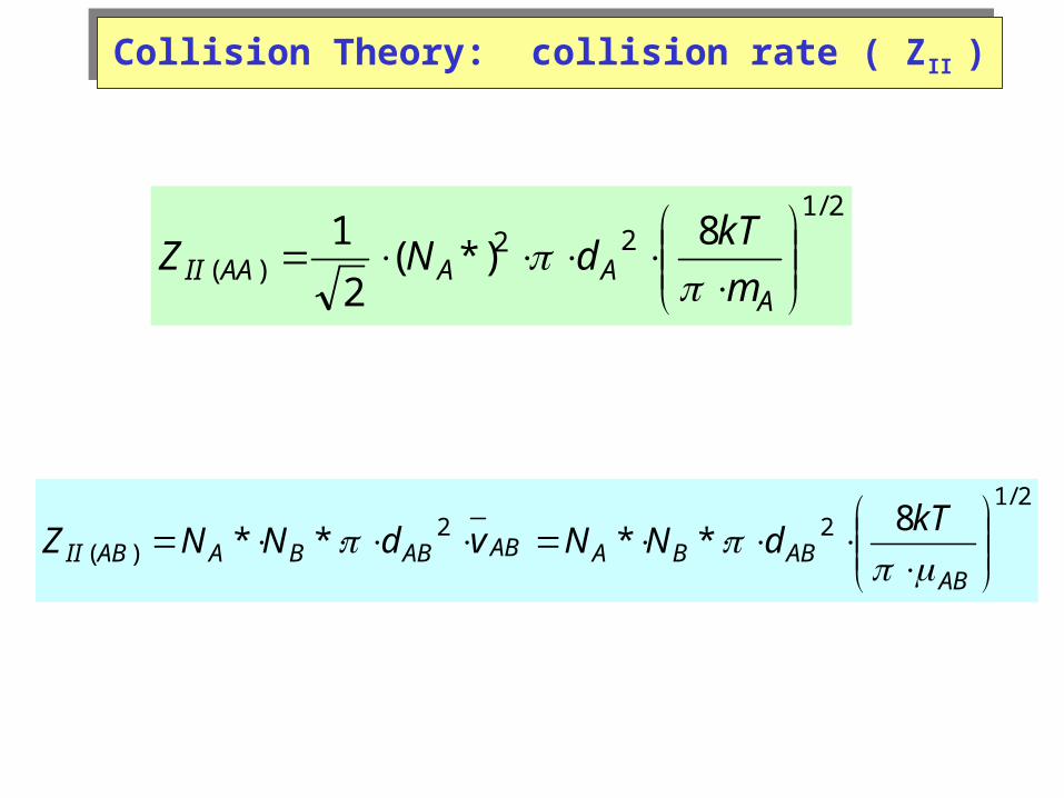
Collision Theory: collision rate ( ZII )Collision Theory: collision rate ( ZII )
2/122
)(8
*)(2
1
A
AAAAII m
kTdNZ
2/122
)(8
****
AB
ABBAABABBAABIIkT
dNNvdNNZ
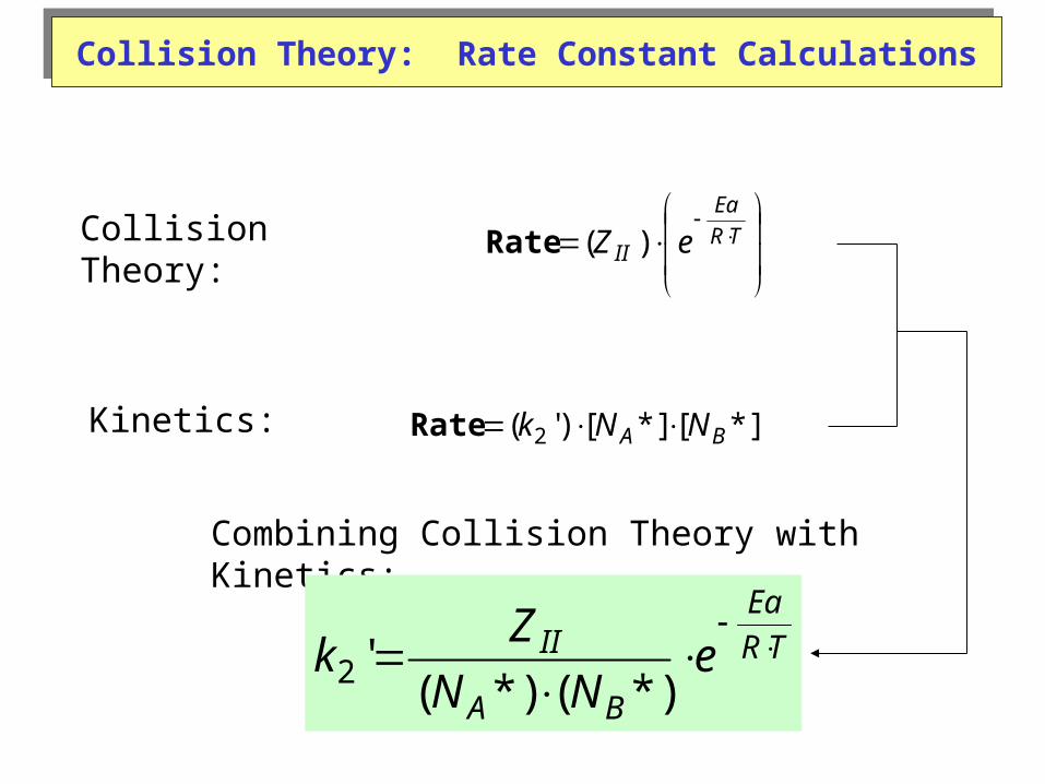
Collision Theory: Rate Constant CalculationsCollision Theory: Rate Constant Calculations
Collision Theory:
TR
Ea
II eZ )(Rate
Kinetics: *][*][)'( 2 BA NNk Rate
Combining Collision Theory with Kinetics:
TR
Ea
BA
II eNN
Zk
*)(*)('2

Collision Theory: Rate Constant CalculationsCollision Theory: Rate Constant Calculations
A-A Collisions
TR
Ea
AA e
m
Tkdk
2/12
28
2
1'
m2 m s-1 per molecule
mol
molecule
m
dm
1
10022.6
1
10 23
3
33
TR
Ea
AAAA e
m
Tkd
Lk
2/12
3
)(28
2
10
Units of k: dm3 mol-1 s-1 M-1 s-1

Collision Theory: Rate Constant CalculationsCollision Theory: Rate Constant Calculations
A-B Collisions
TR
Ea
ABABAB e
TkdLk
2/123
)(28
10
Units of k: dm3 mol-1 s-1 M-1 s-1
2BA
ABdd
d
BA
BAAB mm
mm

Collision Theory: Rate Constant CalculationsCollision Theory: Rate Constant Calculations
Consider: 2 NOCl(g) 2NO(g) + Cl2(g) T = 600. K
Ea = 103 kJ/mol dNOCl = 283 pm (hard-sphere diameter)
Calculate the second order rate constant.

mass ratio k2 / M s-1 Reaction Ea / kJ mol-1
atom-1/atom-2 atom-1 + atom-2-CO2- ---> atom-1-atom-2 + CO2
-
1 1.20E+08 H + HCO2- ---> H2 + CO2
-
0.5 2.30E+07 H + DCO2- ---> HD + CO2
-
0.11 3.40E+06 Mu + HCO2- ---> MuH + CO2
- 33
0.056 9.90E+05 Mu + DCO2- ---> MuD + CO2
- 39
Simple Collision Theory: Comparison of Muonium/Hydrogen/Deuterium Abstractions
0.0E+00
2.0E+07
4.0E+07
6.0E+07
8.0E+07
1.0E+08
1.2E+08
1.4E+08
0.00 0.20 0.40 0.60 0.80 1.00
mass ratio
k /
M-1
s-1
http://www.ubc.ca/index.html
Transition State TheoryTransition State Theory
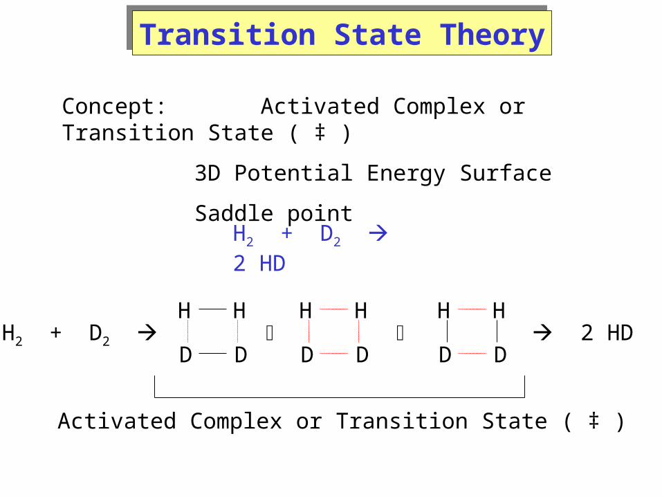
Concept: Activated Complex or Transition State ( ‡ )
3D Potential Energy Surface
Saddle point
H H
DD
H H
DD
H H
DD
H2 + D2 2 HD
H2 + D2 2 HD
Activated Complex or Transition State ( ‡ )
Potential Energy SurfacesPotential Energy Surfaces
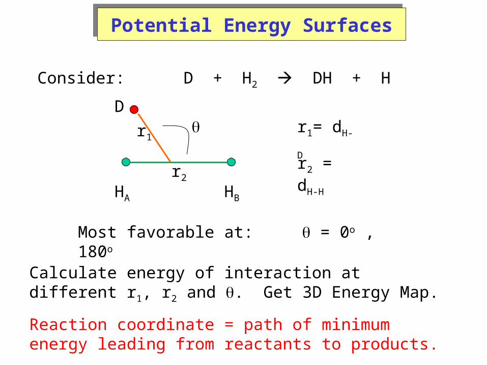
Consider: D + H2 DH + H
D
HA HB
r2
r1 r1= dH-D
r2 = dH-H
Most favorable at: = 0o , 180o
Calculate energy of interaction at different r1, r2 and . Get 3D Energy Map.
Reaction coordinate = path of minimum energy leading from reactants to products.
Reactions in SolutionsReactions in Solutions
Compared to gaseous reactions, reactions in solutions require diffusion through the solvent molecules.
The initial encounter frequencies should be substantially higher for gas collisions.
However, in solutions, though initial encounters are lower, but once the reactants meet, they get trapped in “solvent cages”, and could have a great number of collisions before escaping the solvent cage.

Diffusion Controlled SolutionsDiffusion Controlled Solutions
Smoluchowski (1917): D = diffusion coefficient
)(4 BAABdiff DDLdk
a
TkD
6
3
8 TRkdiff
a = radius;
= viscosity

Diffusion Controlled (Aqueous) Reactions
viscosity
25C 0.8904103 kg m
1 s1 95C 0.297510
3 kg m1 s
1
T1 25 273.15( ) Kk
8R T
3 R 8.3145J mol1 K
1T2 95 273.15( ) K
k25C8 R T1
3 25C k95C
8 R T2
3 95C
k25C 7.42 109 L mol
1 s1 k95C 2.74 10
10 L mol1 s
1
Arrhenius Equation: k A e
Ea
R T kJ 103
J
EaR T1 T2T2 T1
lnk25C
k95C
Ea 1.7 10
4 J mol1 Ea 17kJ mol
1
Therefore all aqueous solutions whose rate is determined by thediffusion of species should have an Activation Energy of about 17kJ/mol.
Diff-paper
Quantum Mechanical TunnelingQuantum Mechanical Tunneling
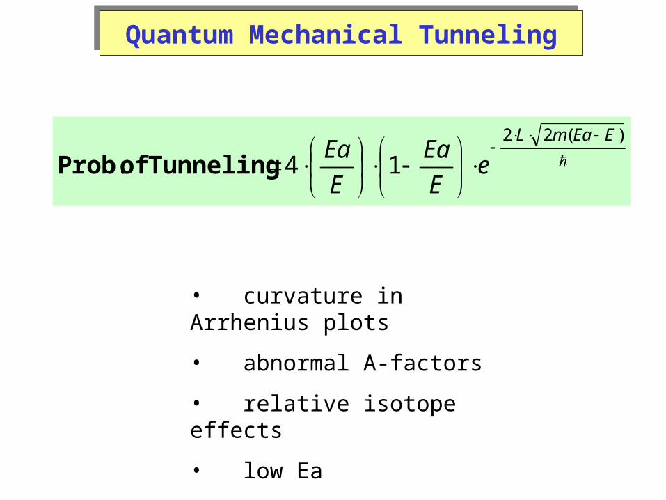
)(22
14EEamL
eE
Ea
E
Ea
Tunneling of Prob.
• curvature in Arrhenius plots
• abnormal A-factors
• relative isotope effects
• low Ea
Boltzmann’s Concepts of Reaction RatesBoltzmann’s Concepts of Reaction Rates
Velocities
Collision Num bers M ean Free Path Viscosities
Derivations Energies
M axw ell-Boltzm ann Distribution
Barom etric Form ulation
Boltzm ann Distribution
222/3
3
4/ ua
D
euadu
NdN
x
naverage
n
N
dNxx )(

Theories of Reaction RatesTheories of Reaction Rates
Collision Param eters
Potential E-surfaces
Unim olecular Reactions
M uonium Kinetics
QM Tunnelling
Isotope Effects
Reactions in Solutions Diffusion Controlled
Partition Functions
Transition State T heory TD T reatm ent of TST
Collision Theory Hard Sphere Diam eters
Arrhenius Concept
TR
Ea
ABABAB e
TkdLk
2/1
23)(2
810
3
8 TRkdiff