arX

iv:h

ep-p

h/03

1015

9v3

9 A

pr 2

004

IFT-25-03 FUT-03-02

UCRHEP-T364

TOKUSHIMA Report

(hep-ph/0310159)

Probing Anomalous Top-Quark Couplings Induced

by Dim.6 Operators at Photon Colliders

Bohdan GRZADKOWSKI 1), a), Zenro HIOKI 2), b),

Kazumasa OHKUMA 3), c) and Jose WUDKA 4), d)

1) Institute of Theoretical Physics, Warsaw University

Hoza 69, PL-00-681 Warsaw, POLAND

and

CERN, Department of Physics

Theory Division

1211 Geneva 23, Switzerland

2) Institute of Theoretical Physics, University of Tokushima

Tokushima 770-8502, JAPAN

3) Department of Management Science, Fukui University of Technology

Fukui 910-8505, JAPAN

4) Department of Physics, University of California

Riverside CA 92521-0413, USA

ABSTRACT

Possible anomalous top-quark couplings induced by SU(2)×U(1) gauge-invar-

iant dimension-6 effective operators were studied in the process of tt productions

and decays at polarized γγ colliders. Two CP -violating asymmetries, a linear-

polarization asymmetry and a circular-polarization asymmetry, were computed in-

cluding both non-standard ttγ and γγH couplings. An optimal-observable analysis

for the process γγ → tt → ℓ± · · · was performed in order to estimate the precision

for determination of all relevant non-standard couplings, including the anomalous

tbW coupling.

PACS: 14.60.-z, 14.65.Ha, 14.70.Bh

Keywords: anomalous top-quark couplings, γγ colliders

a)E-mail address: bohdan.grzadkowski@fuw.edu.plb)E-mail address: hioki@ias.tokushima-u.ac.jpc)E-mail address: ohkuma@ccmails.fukui-ut.ac.jpd)E-mail address: jose.wudka@ucr.edu

1. Introduction

A lot of data have been accumulated on the top-quark ever since its discovery [1].

However, it still remains an open question whether the top-quark couplings obey

the Standard-Model (SM) scheme of the electroweak forces or there exists a contri-

bution from some non-standard physics. Next-generation e+e− linear colliders are

expected to work as top-quark factories, and therefore a lot of attention has been

paid to study top-quark interactions through ee → tt (see, e.g., [2, 3] and their

reference lists).

An interesting option for e+e− machines could be that of photon-photon colli-

sions, where initial energetic photons are produced through electron and laser-light

backward scattering [4, 5]; such a collider presents remarkable advantages for the

study of CP violation. In the case of ee collisions, the only initial states that are

relevant are CP -even states |eL/ReR/L〉 under the usual assumption that the elec-

tron mass can be neglected and that the leading contributions to tt production

come from s-channel vector-boson exchanges. Therefore all CP -violating observ-

ables must be constructed from final-particle momenta/polarizations. In contrast,

a γγ collider offers a unique possibility of preparing the polarization of the incident

photon beams, which can be used to construct CP -violating asymmetries without

relying on final-state information.

This is why a number of authors have considered top-quark production and de-

cays in γγ collisions in order to study i) Higgs-boson couplings to the top-quark and

photon [6]-[12], or ii) anomalous top-quark couplings to photon [13]-[15]. However,

what is supposed to be observed in real experiments are combined signals that

originate both from the process of top-quark production, and in addition, from

its decays. In this sense, we have to conclude that in general those previous pa-

pers are not realistic enough. Therefore here we will consider γγ → tt → ℓ±X

including all possible non-standard interactions together (production and decay),

and perform comprehensive analysis as model-independently as possible within the

effective-Lagrangian framework of Buchmuller and Wyler [16].

The paper is organized as follows. In sec.2 we will briefly describe a framework

for our effective-Lagrangian approach. Section 3 will be devoted to determination of

– 2 –

the operator set relevant for the tt production/decay processes, and the Feynman

rules they induce. Based on them we compute two polarization asymmetries in

sec.4, and carry out an optimal-observable analysis aiming to determine all the

unknown parameters simultaneously in sec.5. Then we summarize our results in

the final section. For completeness, in the appendix we collect formulas that are

needed to describe the Stokes parameters for the initial photon beams. There we

also present some other formulas which are necessary for the calculation of the

cross sections σ(γγ → tt → ℓ±X). Throughout this work, we use FORM [17] for

main algebraic calculations.

2. Framework

In this article we use a model-independent technique based on effective low-energy

Lagrangian [16, 18] to describe possible new-physics effects. In this approach, we

are supposed to consider the SM Lagrangian modified by the addition of a series of

SU(2) × U(1) gauge-invariant operators whose coefficients parameterize the low-

energy effects of the underlying high-scale physics.

Assuming that the heavy degrees of freedom decouple implies that the effective

operators have coefficients suppressed by appropriate inverse powers of Λ, where

Λ expresses the energy scale of new physics [19]. If Λ ≫ v ∼ 250 GeV then

the leading effects are generated by operators of mass-dimension 6 (the dimension

5 operator violates the lepton-number conservation and therefore it is irrelevant

hereafter) [16]:

Leff = LSM +1

Λ2

∑

i

(αiOi + h.c.). (1)

If the high-scale theory is a weakly-coupled gauge theory, one can show that coeffi-

cients αi of the operators that may be generated at the tree level of the underlying

theory could be O(1) while those that can appear only at the one-loop level of

perturbative expansion must be suppressed by at least the loop-factor 1/(4π)2 [18].

Therefore we will assume all the couplings except those from the SM tree level are

small and take into account neither contributions of order 1/Λn with n > 2 nor

the SM higher-order terms. Below we will refer to application of Leff as to “B&W”

scenario [16]. Given our emphasis on top-quark physics the effects of the first two

– 3 –

fermion generations will be ignored.

In our framework, certain types of anomalous interactions are not included. For

instance, γγZ couplings, which has been studied in [20], is one of those couplings

since it is not on the list of SU(3)× SU(2)×U(1) invariant dim.6 operators (such

an operator will appear with a suppression factor of 1/Λ4 and can be ignored).

An extended ttH coupling is not taken into account either, since the other end

of the Higgs propagator in γγ → H → tt is a pure non-standard γγH vertex,

which requires that the ttH coupling should come from the SM tree level within

our approximation.

Before going to the next section, there is an important comment in order.

Even though our approach is model independent, one should keep in mind that we

assume Λ ≫ v. Consequently for the process considered here our results should not

be directly applicable in the context of, e.g., two Higgs-doublet model with extra

scalar bosons having their masses of O(v). That kind of non-standard interactions

would lead to non-local form-factors that cannot be accommodated within our

present framework. This is because of the virtual and therefore off-shell top-quark

line that is present in the amplitudes for γγ → tt. Note that this is quite in contrast

to ee → γ/Z → tt case, where for a given√s we are able to write down the most

general invariant amplitude with constant form factors because all the kinematic

variables are fixed.

3. Anomalous couplings from dim.6 operators

Within the B&W scenario, the following dim.6 operators could contribute to the

continuum top-quark production process γγ → tt:

OuB = iuγµDνuBµν , OqB = iqγµDνqB

µν ,OqW = iqτ iγµDνqW

i µν , O′uB = (qσµνu)ϕBµν ,

OuW = (qσµντ iu)ϕWi µν ,(2)

where we have adopted the notation from ref.[16]. Each of the above operators

contains both CP -violating and CP -conserving parts.

These operators, however, are not independent. Using the Bianchi identities

and SM equations of motion we find:

OuB = −1

4[ iΓu(O′

uB + g′Ouϕ) + h.c. ]− ig′

2Oϕu

– 4 –

+ 4-fermion operators + total derivative, (3)

OqB =1

4[ iΓu(O′

uB + g′Ouϕ) + iΓd(O′dB + g′Odϕ) + h.c. ]

− ig′

2O(1)

ϕq + 4-fermion operators + total derivative, (4)

OqW =1

4[ iΓu(OuW − gOuϕ) + iΓd(OdW + gOdϕ) + h.c. ]

− ig

2O(3)

ϕq + 4-fermion operators + total derivative, (5)

where Γu,d are the Yukawa couplings for up- and down-type quarks, respectively.♯1

These relations imply that the operators OuB, OqB and OqW are redundant and

can be dropped, which means the set of relevant operators is reduced to

O′uB = (qσµνu)ϕBµν , OuW = (qσµντ iu)ϕWi µν . (6)

This reduction is important, as it allows to determine the minimal set of operators

that are relevant for the process considered here. In practice, it can drastically

decrease the effort that otherwise would be necessary to obtain the final and correct

result. In particular, it shows that the contact interactions of the type ttγγ should

be dropped.

On the other hand, the following operators contribute to γγ → tt through the

resonant s-channel Higgs-boson exchange:

OϕW = (ϕ†ϕ)W iµνW

i µν , OϕW = (ϕ†ϕ)W iµνW

i µν/2,

OϕB = (ϕ†ϕ)BµνBµν , OϕB = (ϕ†ϕ)BµνB

µν/2,

OWB = (ϕ†τ iϕ)W iµνB

µν , OWB = (ϕ†τ iϕ)W iµνB

µν .

(7)

The operators that contain the dual tensors (e.g., Bµν ≡ ǫµναβBαβ/2 with ǫ0123 =

+1) are CP odd while the remaining are CP even.

These operators lead to the following Feynman rules for on-shell photons, which

are necessary for our later calculations:

(1) CP -conserving ttγ vertex √2

Λ2vαγ1 k/ γµ, (8)

(2) CP -violating ttγ vertex

i

√2

Λ2vαγ2 k/ γµγ5, (9)

♯1Notice an omission of the term iϕ†↔

Dβ ϕ/2 in eq.(2.14) of [16].

– 5 –

(3) CP -conserving γγH vertex

− 4

Λ2vαh1 [ (k1k2)gµν − k1νk2µ ], (10)

(4) CP -violating γγH vertex

8

Λ2vαh2 k

ρ1k

σ2 ǫρσµν , (11)

where k and k1,2 are incoming photon momenta, and αγ1,γ2,h1,h2 are defined as

αγ1 ≡ sin θWRe(αuW ) + cos θWRe(α′uB), (12)

αγ2 ≡ sin θW Im(αuW ) + cos θW Im(α′uB), (13)

αh1 ≡ sin2 θWRe(αϕW ) + cos2 θWRe(αϕB)− 2 sin θW cos θWRe(αWB), (14)

αh2 ≡ sin2 θWRe(αϕW ) + cos2 θWRe(αϕB)− sin θW cos θWRe(αWB). (15)

In our notation, the standard-model f fγ coupling is given by

eQfγµ,

where e is the proton charge and Qf is f ’s electric charge in e unit (e.g., Qu = 2/3).

The top-quark decay vertex is also affected by some dim.6 operators. For the on-

mass-shell W boson it will be sufficient to consider just the following tbW amplitude

since other possible terms do not interfere with the SM tree-level vertex when mb

is neglected:

Γ µWtb = − g√

2u(pb)

[

γµfL1 PL − iσµνkν

MWfR2 PR

]

u(pt), (16)

where PL,R ≡ (1∓ γ5)/2, and fL1 and fR

2 are given by

fL1 = 1 +

v

Λ2

[ mt

2αDu − 2vα(3)

ϕq

]

, (17)

fR2 = − v

Λ2MW

[ 4

gαuW +

1

2αDu

]

, (18)

with αDu and α(3)ϕq being the coefficients of the following operators:♯2.

ODu = (qDµu)Dµϕ, O(3)

ϕq = i(ϕ†Dµτiϕ)(qγµτ iq). (19)

Finally, the νℓW vertex is assumed to receive negligible contributions from physics

beyond the SM.♯2Note that there is another potential source of contribution, which may come from ODu =

(Dµq)uDµϕ. However, this operator could be eliminated using equations of motion; therefore, it

is neglected hereafter. We thank Ilya Ginzburg for pointing this to us.

– 6 –

4. Polarization asymmetries

We are now ready to calculate the cross section of γγ → tt(→ ℓ±X). The work

is straightforward and we carried it out via FORM [17] as mentioned in sec.1.

The analytical results are however too long to show in this paper. We therefore

refrain from showing them here and we will present only some general formulas

in appendix A1. As a direct application of those calculations, in this section we

study CP -violating asymmetries. CP -violation phenomena would be an interesting

indication of some new physics since SM contribution is negligible in the top-quark

couplings.

As mentioned in the Introduction, we can form CP -violating asymmetries by

adjusting initial-state polarizations. These are characterized by the initial electron

and positron longitudinal-polarizations Pe and Pe, the average helicities of the

initial-laser-photons Pγ and Pγ, and their maximum average linear-polarizations

Pt and Pt with the azimuthal angles ϕ and ϕ (defined the same way as in [4]). Pγ,t

and Pγ,t have to satisfy

0 ≤ P 2γ + P 2

t ≤ 1, 0 ≤ P 2γ + P 2

t ≤ 1. (20)

Specifically we consider the following CP -violating asymmetries:♯3

Alin ≡ σ(χ = +π/4)− σ(χ = −π/4)

σ(χ = +π/4) + σ(χ = −π/4)(21)

and

Acir ≡σ(++)− σ(−−)

σ(++) + σ(−−), (22)

where σ(χ = ±π/4) means the total cross section of γγ → tt with Pe = Pe = 1,

Pt = Pt = Pγ = Pγ = 1/√2 and χ ≡ ϕ− ϕ = ±π/4, while σ(±±) corresponds to

the one with Pe = Pe = Pγ = Pγ = ±1 (which means Pt = Pt = 0). They were

computed as functions of the Higgs-boson mass for

√see = 500 GeV, Λ = 1 TeV, y0 = y0 = 4.828,

αγ2 = αh2 = 0.1

and using the SM expression for the Higgs-boson width. The results are shown in

Figs.1 and 2.

♯3These were used previously in [8] in order to study the CP property of the Higgs bosonproduced in γγ → H . Alin was also used in [13, 14] for studying the CP -violating ttγ coupling.

– 7 –

100 200 300 400 500 600 700mHiggs

-0.08

-0.06

-0.04

-0.02

0

0.02

A lin

[GeV]

Figure 1: CP -violating linear-polarization asymmetry Alin as a function of theHiggs-boson mass computed for

√see = 500 GeV, Λ = 1 TeV, y0 = y0 = 4.828,

αγ2 = αh2 = 0.1, Pe = Pe = 1, Pt = Pt = Pγ = Pγ = 1/√2 and χ ≡ ϕ− ϕ = ±π/4.

The sharp peak in each asymmetry comes, of course, from the Higgs-boson

pole, where the signal will be easily observed. The resonance region has been

already studied in great details in existing literature [6]-[12]. Here we will study

the possibility of extracting a meaningful signal when the average√sγγ is far from

the Higgs-boson mass. For the parameters adopted above one can find approximate

formulas that illustrate sensitivity to CP -violating coefficients αγ2 and αh2:

(1) mH = 100 GeV

Alin = −(8.8αγ2 + 4.2αh2)× 10−2, (23)

Acir = −5.2× 10−6 αh2. (24)

(2) mH = 300 GeV

Alin = −(8.8αγ2 + 11αh2)× 10−2, (25)

Acir = −8.5 × 10−2 αh2. (26)

(3) mH = 500 GeV

Alin = −(8.8αγ2 − 8.1αh2)× 10−2, (27)

– 8 –

100 200 300 400 500 600 700mHiggs

-0.6

-0.5

-0.4

-0.3

-0.2

-0.1

0

A cir

[GeV]

Figure 2: CP -violating circular-polarization asymmetry Acir as a function of theHiggs-boson mass computed for

√see = 500 GeV, Λ = 1 TeV, y0 = y0 = 4.828,

αh2 = 0.1, and Pe = Pe = Pγ = Pγ = ±1.

Acir = −0.24αh2. (28)

Note that because of the γ5 factor in the CP -violating ttγ vertex (9) its interfer-

ence with the SM amplitude vanishes when the initial photons have pure circular

polarizations [13]. This is why the αγ2 contribution to Acir is zero.

Since the asymmetries are all small, their expected statistical errors in actual

measurements can be computed by

∆Alin,cir ≃ 1/√

Ntt (29)

and consequently their statistical significances are estimated as

NSD ≡ |A|/∆A ≃ |A|√

Ntt. (30)

We estimate Ntt ∼ 36,000 and 21,000 events for the linear and circular polar-

izations respectively assuming that a luminosity of Leffee ≡ ǫLee = 500 fb−1 can

be reached for each mode (ǫ denotes the relevant detection efficiency and Lee is

the integrated luminosity). In this case deviations from the SM will be observable

provided the coefficients αγ2 and αh2 are of the order of 0.1.

– 9 –

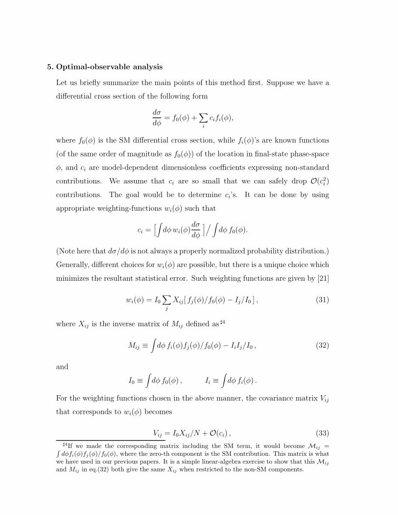
5. Optimal-observable analysis

Let us briefly summarize the main points of this method first. Suppose we have a

differential cross section of the following form

dσ

dφ= f0(φ) +

∑

i

cifi(φ),

where f0(φ) is the SM differential cross section, while fi(φ)’s are known functions

(of the same order of magnitude as f0(φ)) of the location in final-state phase-space

φ, and ci are model-dependent dimensionless coefficients expressing non-standard

contributions. We assume that ci are so small that we can safely drop O(c2i )

contributions. The goal would be to determine ci’s. It can be done by using

appropriate weighting-functions wi(φ) such that

ci =[

∫

dφwi(φ)dσ

dφ

]/

∫

dφ f0(φ).

(Note here that dσ/dφ is not always a properly normalized probability distribution.)

Generally, different choices for wi(φ) are possible, but there is a unique choice which

minimizes the resultant statistical error. Such weighting functions are given by [21]

wi(φ) = I0∑

j

Xij [ fj(φ)/f0(φ)− Ij/I0 ] , (31)

where Xij is the inverse matrix of Mij defined as ♯4

Mij ≡∫

dφ fi(φ)fj(φ)/f0(φ)− IiIj/I0 , (32)

and

I0 ≡∫

dφ f0(φ) , Ii ≡∫

dφ fi(φ) .

For the weighting functions chosen in the above manner, the covariance matrix Vij

that corresponds to wi(φ) becomes

Vij = I0Xij/N +O(ci) , (33)

♯4If we made the corresponding matrix including the SM term, it would become Mij =∫

dφfi(φ)fj(φ)/f0(φ), where the zero-th component is the SM contribution. This matrix is whatwe have used in our previous papers. It is a simple linear-algebra exercise to show that this Mij

and Mij in eq.(32) both give the same Xij when restricted to the non-SM components.

– 10 –

where N is the total number of collected events. Its diagonal elements give expected

statistical uncertainty for measurements of ci as

|∆ci| =√

Vii. (34)

We are going to apply this technique to the final-lepton angular and energy

distribution of γγ → tt → ℓ+X

dσ

dEℓd cos θℓ= fSM(Eℓ, cos θℓ) + αγ1fγ1(Eℓ, cos θℓ) + αγ2fγ2(Eℓ, cos θℓ)

+ αh1fh1(Eℓ, cos θℓ) + αh2fh2(Eℓ, cos θℓ) + αdfd(Eℓ, cos θℓ) (35)

in the ee-CM frame. Here fSM denotes the standard-model contribution, fγ1,γ2

describe, respectively, the anomalous CP -conserving- and CP -violating-ttγ-vertices

contributions, fh1,h2 those generated by the anomalous CP -conserving and CP -

violating γγH-vertices, and fd that by the anomalous tbW -vertex with

αd = Re(fR2 ).

See the Appendix for details of our calculation framework.

The covariance matrix Vij ∝ Xij determines our ability to measure the coeffi-

cients ci. However in the case considered here, it turns out that our results for Vij

are very unstable: even a tiny fluctuation of Mij changes Xij significantly. This in-

dicates that some of fi have similar shapes ♯5 and therefore their coefficients cannot

be easily disentangled. The only option in such a case is to refrain from determining

all the couplings at once through this process alone. Therefore hereafter we assume

that some of ci’s have been measured in other processes (e.g. in ee → tt → ℓ±X).

In order to carry out these studies numerically, we first give full elements of

MIJ =∫

dEℓd cos θℓ fI(Eℓ, cos θℓ)fJ(Eℓ, cos θℓ)/f1(Eℓ, cos θℓ),

where I, J = 1, · · · , 6 correspond to SM, γ1, γ2, h1, h2 and d respectively as our

basis. The (i, j) elements (i, j = 2 ∼ 6) of M’s inverse matrix coincide with Xij

appearing in eq.(31) as mentioned in footnote 3.

♯5Note that if two fi functions were proportional to each other then the matrix Mij would havea vanishing determinant, and therefore its inverse Xij could not be determined.

– 11 –

(1) Linear Polarization

We took Pe = Pe = 1, Pt = Pt = Pγ = Pγ = 1/√2 and χ = π/4, which

were used to compute Alin in the previous section as typical linear-polarization

parameters.

1-1) mH = 100 GeV

M11 = 0.810 · 101, M12 = 0.173 · 102, M13 = −0.703,M14 = −0.319 · 101, M15 = −0.337, M16 = 0,M22 = 0.377 · 102, M23 = −0.153 · 101, M24 = −0.627 · 101,M25 = −0.730, M26 = 0.125 · 101, M33 = 0.638 · 10−1,M34 = 0.248, M35 = 0.305 · 10−1, M36 = −0.683 · 10−1,M44 = 0.183 · 101, M45 = 0.122, M46 = 0.135 · 101,M55 = 0.149 · 10−1, M56 = −0.263 · 10−1, M66 = 0.392 · 101.

(36)

1-2) mH = 300 GeV

M11 = 0.810 · 101, M12 = 0.173 · 102, M13 = −0.703,M14 = −0.790 · 101, M15 = −0.152 · 101, M16 = 0,M22 = 0.377 · 102, M23 = −0.153 · 101, M24 = −0.156 · 102,M25 = −0.314 · 101, M26 = 0.125 · 101, M33 = 0.638 · 10−1,M34 = 0.616, M35 = 0.128, M36 = −0.683 · 10−1,M44 = 0.112 · 102, M45 = 0.176 · 101, M46 = 0.332 · 101,M55 = 0.309, M56 = 0.260, M66 = 0.392 · 101.

(37)

1-3) mH = 500 GeV

M11 = 0.810 · 101, M12 = 0.173 · 102, M13 = −0.703,M14 = 0.374 · 101, M15 = −0.221 · 101, M16 = 0,M22 = 0.377 · 102, M23 = −0.153 · 101, M24 = 0.737 · 101,M25 = −0.425 · 101, M26 = 0.125 · 101, M33 = 0.638 · 10−1,M34 = −0.293, M35 = 0.166, M36 = −0.683 · 10−1,M44 = 0.251 · 101, M45 = −0.165 · 101, M46 = −0.155 · 101,M55 = 0.110 · 101, M56 = 0.122 · 101, M66 = 0.392 · 101.

(38)

(2) Circular Polarization

What we took as circular-polarization parameters are also those used for Acir:

Pe = Pe = Pγ = Pγ = 1.

2-1) mH = 100 GeV

M11 = 0.460 · 101, M12 = 0.996 · 101, M13 = 0,M14 = −0.152 · 101, M15 = −0.240 · 10−4, M16 = 0,M22 = 0.219 · 102, M23 = 0, M24 = −0.306 · 101,M25 = −0.481 · 10−4, M26 = 0.611, M33 = 0,M34 = 0, M35 = 0, M36 = 0,M44 = 0.748, M45 = 0.122 · 10−4, M46 = 0.660,M55 = 0.198 · 10−9, M56 = 0.114 · 10−4, M66 = 0.229 · 101.

(39)

– 12 –

2-2) mH = 300 GeV

M11 = 0.460 · 101, M12 = 0.996 · 101, M13 = 0,M14 = −0.392 · 101, M15 = −0.389, M16 = 0,M22 = 0.219 · 102, M23 = 0, M24 = −0.793 · 101,M25 = −0.781, M26 = 0.611, M33 = 0,M34 = 0, M35 = 0, M36 = 0,M44 = 0.497 · 101, M45 = 0.502, M46 = 0.171 · 101,M55 = 0.511 · 10−1, M56 = 0.181, M66 = 0.229 · 101.

(40)

2-3) mH = 500 GeV

M11 = 0.460 · 101, M12 = 0.996 · 101, M13 = 0,M14 = 0.168 · 101, M15 = −0.110 · 101, M16 = 0,M22 = 0.219 · 102, M23 = 0, M24 = 0.338 · 101,M25 = −0.221 · 101, M26 = 0.611, M33 = 0,M34 = 0, M35 = 0, M36 = 0,M44 = 0.920, M45 = −0.634, M46 = −0.728,M55 = 0.436, M56 = 0.537, M66 = 0.229 · 101.

(41)

All the elements Mij above are given in units of fb. In these results, the third

components of M for the circular polarization vanish as was mentioned in sec.4.

Also, in accordance with the decoupling theorem shown in [22], the elements M16

are always zero within our approximation of neglecting contributions quadratic in

non-standard interactions and treating the decaying t and W as on-shell particles.

When estimating the statistical uncertainty in simultaneous measurements of,

e.g., αγ1 and αh1 (assuming all other coefficients are known), we need only the

components with indices 1, 2 and 4. Let us express the resultant uncertainties as

∆α[3]γ1 and ∆α

[3]h1, where “3” means that we took account of the input Mij up to

three decimal places. In order to see how stable the results are, we also computed

∆α[2]γ1 and ∆α

[2]h1 by rounding Mij off to two decimal places. Then, if both of the

deviations |∆α[3]γ1,h1 −∆α

[2]γ1,h1|/∆α

[3]γ1,h1 are less than 10 %, we adopted the results

as stable solutions. Therefore, the ambiguity of the following results ∆αi, which

are ∆α[3]i , is at most 10 %.

1) Linear Polarization

What we obtained as stable solutions for linear polarization are

• Independent of mH

∆αγ2 = 73/√

Nℓ, ∆αd = 1.9/√

Nℓ, (42)

– 13 –

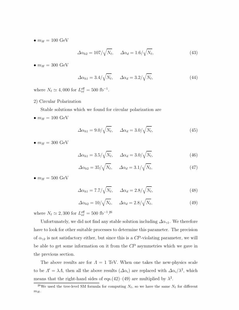
• mH = 100 GeV

∆αh2 = 107/√

Nℓ, ∆αd = 1.6/√

Nℓ, (43)

• mH = 300 GeV

∆αh1 = 3.4/√

Nℓ, ∆αd = 3.2/√

Nℓ, (44)

where Nℓ ≃ 4, 000 for Leffee = 500 fb−1.

2) Circular Polarization

Stable solutions which we found for circular polarization are

• mH = 100 GeV

∆αh1 = 9.0/√

Nℓ, ∆αd = 3.0/√

Nℓ, (45)

• mH = 300 GeV

∆αh1 = 3.5/√

Nℓ, ∆αd = 3.0/√

Nℓ, (46)

∆αh2 = 35/√

Nℓ, ∆αd = 3.1/√

Nℓ, (47)

• mH = 500 GeV

∆αh1 = 7.7/√

Nℓ, ∆αd = 2.8/√

Nℓ, (48)

∆αh2 = 10/√

Nℓ, ∆αd = 2.8/√

Nℓ, (49)

where Nℓ ≃ 2, 300 for Leffee = 500 fb−1.♯6

Unfortunately, we did not find any stable solution including ∆αγ1. We therefore

have to look for other suitable processes to determine this parameter. The precision

of αγ2 is not satisfactory either, but since this is a CP -violating parameter, we will

be able to get some information on it from the CP asymmetries which we gave in

the previous section.

The above results are for Λ = 1 TeV. When one takes the new-physics scale

to be Λ′ = λΛ, then all the above results (∆αi) are replaced with ∆αi/λ2, which

means that the right-hand sides of eqs.(42)–(49) are multiplied by λ2.

♯6We used the tree-level SM formula for computing Nℓ, so we have the same Nℓ for differentmH .

– 14 –

It should be mentioned here that the above estimation of expected errors does

not take into account a possible background. However the top-quark tagging in

the one-lepton and six-jets final state is relatively straightforward and therefore

should not increase the uncertainties found above very dramatically. Of course, in

the real experiment, one will have to redo the analysis taking into account not only

the background, but also all the systematic errors which are unknown at present.

Therefore the fully realistic analysis cannot be performed at this moment.

6. Summary and discussion

We have studied here beyond-the-SM effects in the process γγ → tt(→ ℓ+X) for

arbitrarily-polarized photon beams, taking advantage of the fact that one can con-

trol polarizations of the incoming photon beams. Non-standard interactions have

been parameterized through dim.6 local and gauge symmetric effective operators

a la Buchmuller and Wyler [16] toward the first realistic comprehensive model-

independent analysis of the process. We listed all the necessary operators and the

corresponding Feynman rules. It was shown that in the list of operators that seem

to contribute there are some which are redundant and should be dropped in the

analysis. Assuming that those new-physics (NP) effects are small, we have kept

only terms linear in modification of the SM tree vertices.

We first computed two CP -violating polarization asymmetries for linear and

circular photon polarizations, and found there are good chances of detecting their

signals. We then applied the optimal-observable technique to the final-lepton-

momentum distribution, and estimated statistical significances of measuring each

NP-parameters. Unfortunately, we had to conclude that it is never realistic to try

to determine all the independent NP-parameters at once through γγ → tt → ℓ±X

alone, but still we would be able to perform useful analysis if we could utilize

complementary information collected in other independent processes.

We have not discussed here a possible background. This is mainly because iden-

tifying the tt final state in semileptonic-hadronic decays is easy, since we always

have a very energetic charged lepton and the other (anti)top quark decaying purely

hadronically with an invariant mass of mt. That is, the tagging in this particular

final state will be relatively easy. However, some comments on background esti-

– 15 –

mation will be helpful. Although the most serious background is W -boson pair

productions and indeed its total cross section could be larger than σtot(tt), a ded-

icated simulation study [23] has shown that tt events can be selected with signal-

to-background ratio of 10 by imposing appropriate invariant-mass constraints on

the final-particle momenta.

It should be stressed that for the purpose of future data analysis it is unavoidable

to have a tool which would allow consistently to control all possible effects. For

instance it is conceivable that some non-standard effects from the top-quark decays

would mimic another non-standard interactions from the tt production process,

therefore without an analysis that allows to control all those contribution any

meaningful data analysis would be impossible.

Finally, it should be emphasized here that the effective-operator strategy adopted

in this article is valid only for Λ ≫ v ∼ 250 GeV, in contrast with e+e− → tt →ℓ±X . Should the reaction γγ → tt → ℓ±X exhibit a deviation from the SM predic-

tions that cannot be described properly within this framework, this would be an

indication of a low-energy beyond-the-SM physics, e.g., two Higgs-doublet model

with relatively low mass scale of new scalar degrees of freedom.

ACKNOWLEDGMENTS

One of us (Z.H.) would like to thank Tohru Takahashi for very useful discussion,

Isamu Watanabe for showing some results of their numerical computations, and Eri

Asakawa and Saurabh Rindani for kind correspondence on their works. B.G. thanks

Mikolaj Misiak for useful discussions concerning effective Lagrangians. This work

is supported in part by the State Committee for Scientific Research (Poland) under

grant 1 P03B 078 26 in the period 2004-2006 and the Grant-in-Aid for Scientific

Research No.13135219 from the Japan Society for the Promotion of Science.

APPENDIX

A1. Cross section for γγ → tt → ℓ±X

– 16 –

For photons with definite polarizations the cross section for γγ → tt is given by

dσ(γγ → tt) = C|Mαβǫα(h1)ǫ

β(h2)|2

= CMαβǫα(h1)ǫ

β(h2)M∗ρσǫ

∗ρ(h1)ǫ∗σ(h2), (50)

where C expresses the kinematically-determined part, and h1,2 are the helicities of

the initial two photons:

ǫµ(h1) =1√2(ǫµ1 + ih1ǫ

µ2 ), ǫµ(h2) =

1√2(−ǫµ1 + ih2ǫ

µ2 ) (51)

with ǫµ1 = (0, 1, 0, 0) and ǫµ2 = (0, 0, 1, 0). Since ǫµ(±1) and ǫµ(±1) are

ǫµ(±1) =1√2(ǫµ1 ± iǫµ2 ), ǫµ(±1) =

1√2(−ǫµ1 ± iǫµ2 ),

we can express ǫµ(h1) and ǫµ(h2) as

ǫµ(h1) =∑

a=±1

eaǫµ(a), ǫµ(h2) =∑

a=±1

eaǫµ(a), (52)

where the coefficients are e±1 = (1± h1)/2 and e±1 = (1±h2)/2. In terms of these

quantities, the above cross section is

dσ(γγ → tt) = C∑

a,b,c,d=±1

eaec∗ebed∗MαβM∗ρσǫ

α(a)ǫ∗ρ(c)ǫβ(b)ǫ∗σ(d)

≡ C∑

a,b,c,d=±1

eaec∗ebed∗T ac,bd . (53)

The actual cross section dσ(γγ → tt) measured at experiments is obtained by

multiplying the above cross section with the photon-spectra functions dN/dy and

dN/dy, which work similarly to the parton-distribution functions inside hadrons

and replacing eaec∗ and ebed∗ with the spin density matrices ρ and ρ respectively,

dσ =∑

a,b,c,d=±1

∫

dy dydN(y)

dy

dN(y)

dyρac(y)ρbd(y)dσac,bd(y, y), (54)

where

dσac,bd(y, y) = C T ac,bd(y, y)

is the cross section for two initial photons carrying energy-fraction y and y of those

of e and e, ρ(y) and ρ(y) are expressed in terms of the three Stokes parameters as

ρ(y) =1

2

(

1 + ξ2(y) ξ3(y)− iξ1(y)ξ3(y) + iξ1(y) 1− ξ2(y)

)

, (55)

– 17 –

ρ(y) =1

2

(

1 + ξ2(y) ξ3(y) + iξ1(y)

ξ3(y)− iξ1(y) 1− ξ2(y)

)

(56)

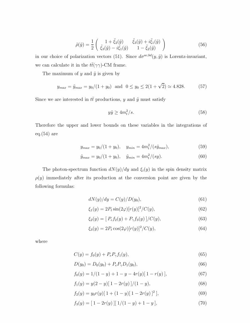
in our choice of polarization vectors (51). Since dσac,bd(y, y) is Lorentz-invariant,

we can calculate it in the tt(γγ)-CM frame.

The maximum of y and y is given by

ymax = ymax = y0/(1 + y0) and 0 ≤ y0 ≤ 2(1 +√2) ≃ 4.828. (57)

Since we are interested in tt productions, y and y must satisfy

yy ≥ 4m2t/s. (58)

Therefore the upper and lower bounds on these variables in the integrations of

eq.(54) are

ymax = y0/(1 + y0), ymin = 4m2t/(symax), (59)

ymax = y0/(1 + y0), ymin = 4m2t/(sy). (60)

The photon-spectrum function dN(y)/dy and ξi(y) in the spin density matrix

ρ(y) immediately after its production at the conversion point are given by the

following formulas:

dN(y)/dy = C(y)/D(y0), (61)

ξ1(y) = 2Pt sin(2ϕ)[r(y)]2/C(y), (62)

ξ2(y) = [ Pef2(y) + Pγf3(y) ]/C(y), (63)

ξ3(y) = 2Pt cos(2ϕ)[r(y)]2/C(y), (64)

where

C(y) = f0(y) + PePγf1(y), (65)

D(y0) = D0(y0) + PePγD1(y0), (66)

f0(y) = 1/(1− y) + 1− y − 4r(y)[ 1− r(y) ], (67)

f1(y) = y(2− y)[ 1− 2r(y) ]/(1− y), (68)

f2(y) = y0r(y)[ 1 + (1− y)[ 1− 2r(y) ]2 ], (69)

f3(y) = [ 1− 2r(y) ][ 1/(1− y) + 1− y ], (70)

– 18 –

r(y) = y/[ y0(1− y) ], (71)

D0(y0) = (1− 4/y0 − 8/y20) ln(1 + y0) + 1/2

+ 8/y0 − 1/[ 2(1 + y0)2 ], (72)

D1(y0) = (1 + 2/y0) ln(1 + y0)− 5/2 + 1/(1 + y0)

− 1/[ 2(1 + y0)2 ], (73)

which are of course common to dN(y)/dy and ξi(y) too.

Finally, combining thus-calculated dσ(γγ → tt) with dΓ (t → ℓX) through the

Kawasaki-Shirafuji-Tsai formula [24], we arrive at the cross section dσ(γγ → tt →ℓ±X):

dσ

dpℓ

≡ dσ

dpℓ

(1 + 2 → t+ · · · → ℓ + · · ·)

= 2∫

dpt

dσ

dpt

(st = n)1

Γt

dΓ

dpℓ

= 2Bℓ

∫

dpt

dσ

dpt

(st = n)1

Γ

dΓ

dpℓ

. (74)

Here dp denotes the Lorentz-invariant phase-space element dp/[ (2π)32p0 ], dΓ/dpℓ

is the spin-averaged top-quark width

dΓ

dpℓ

≡ dΓ

dpℓ

(t → ℓ+ · · ·),

Bℓ ≡ Γ/Γt, and dσ(st = n)/dpt is the single-top-quark inclusive cross section

dσ

dpt

(st = n) ≡ dσ

dpt

(1 + 2 → t+ · · · ; st = n)

with the polarization vector st being replaced with the so-called “effective polar-

ization vector” n

nµ = −[

gµν −ptµptνm2

t

]

∑

spin

∫

dΦ BΛ+γ5γνB

∑

spin

∫

dΦ BΛ+B, (75)

where the spinor B is defined such that the matrix element for t(st) → ℓ + · · · isexpressed as But(pt, st), Λ+ ≡ p/t + mt, dΦ is the relevant final-state phase-space

element, and∑

spin denotes the appropriate spin summation. dΓ (t → ℓX) for the

amplitude (16) is given by

1

Γt

dΓ

dxdω=

1 + β

β

3Bℓ

Wω[

1 + 2Re(fR2 )

√r( 1

1− ω− 3

1 + 2r

) ]

(76)

– 19 –

where r ≡ (MW/mt)2, W ≡ (1 − r)2(1 + 2r), ω ≡ (pt − pℓ)

2/m2t , and x is defined

by the tt CM-frame lepton-energy Eℓ and β ≡√

1− 4m2t/s as

x ≡ 2Eℓ

mt

√

(1− β)/(1 + β).

Note that eq.(74) holds very generally as long as the narrow-width approximation

is applicable to both the top-quark and W -boson propagators.

A2. Cross sections in ee- and γγ-CM frames

Calculations of cross sections are much simpler in γγ-CM frame, while actual exper-

imental measurements are performed in ee-CM frame. Any observables expressed

in these two frames are of course connected via a proper Lorentz transformation.

We summarize here some necessary formulas.

Let us express the lepton energy and scattering angle in ee-CM frame as E and

θ, and those in the γγ-CM frame as E⋆ and θ⋆. Their relation is given by

E⋆ =E(1− β cos θ)√

1− β2, cos θ⋆ =

cos θ − β

1− β cos θ, (77)

where

β = (y − y)/(y + y), (78)

y and y are the energy fractions of e and e carried by the initial photon 1 and 2,

which appeared in eq.(54). The scattering angle is defined as the angle between

the final-lepton ℓ and the initial-photon 1.

Based on these formulas, we have

dσ

dEd cos θ=∫

dy dydN(y)

dy

dN(y)

dy

dσ

dEd cos θ(y, y)

=∫

dy dydN(y)

dy

dN(y)

dyJ(y, y)

dσ

dE⋆d cos θ⋆(y, y), (79)

where the Jacobian J(y, y) is given by

J(y, y) =

√1− β2

1− β cos θ. (80)

dσ(y, y)/(dE⋆d cos θ⋆) is originally a function of E⋆ and cos θ⋆, but they have to

be re-expressed in terms of E and cos θ in eq.(79) through the relations given in

eq.(77).

– 20 –

Finally let us show the integration region for E and cos θ in dσ/(dEd cos θ). It

is easy to confirm

− 1 ≤ cos θ⋆ ≤ +1 ⇐⇒ −1 ≤ cos θ ≤ +1. (81)

On the other hand, the upper and lower bounds of the energy are a bit more

complicated. Since

mtr

2

√

1− β⋆(y, y)

1 + β⋆(y, y)≤ E⋆ ≤ mt

2

√

1 + β⋆(y, y)

1− β⋆(y, y),

where β⋆(y, y) ≡√

1− 4m2t/(yys), one obtains

1

2mtr

√

1− β⋆(y, y)

1 + β⋆(y, y)

√1− β2

1− β cos θ≤ E ≤ 1

2mt

√

1 + β⋆(y, y)

1− β⋆(y, y)

√1− β2

1− β cos θ. (82)

Since the right(left)-hand side takes its maximum (minimum) for y = y = ymax,

we have1

2mtr

√

1− β⋆max

1 + β⋆max

≤ E ≤ 1

2mt

√

1 + β⋆max

1− β⋆max

(83)

for the energy integration in the ee-CM frame, where β⋆max ≡ β⋆(ymax, ymax).

REFERENCES

[1] CDF Collaboration : F. Abe et al., Phys. Rev. Lett. 73 (1994), 225

(hep-ex/9405005); Phys. Rev. D50 (1994), 2966; Phys. Rev. Lett. 74 (1995),

2626 (hep-ex/9503002);

D0 Collaboration : S. Abachi et al., Phys. Rev. Lett. 74 (1995), 2632

(hep-ex/9503003).

[2] D. Atwood, S. Bar-Shalom, G. Eilam and A. Soni, Phys. Rept. 347 (2001), 1

(hep-ph/0006032).

[3] ACFA Linear Collider Working Group Collaboration : K. Abe et al., “Particle

physics experiments at JLC” KEK Report 2001-11 (hep-ph/0109166).

[4] I.F. Ginzburg, G.L. Kotkin, V.G. Serbo and V.I. Telnov, Nucl. Instrum. Meth.

205 (1983) 47.

– 21 –

[5] D.L. Borden, D. Bauer and D.O. Caldwell, SLAC-PUB-5715, UCSB-HEP-92-

01.

[6] B. Grzadkowski and J.F. Gunion, Phys. Lett. B294 (1992), 361

(hep-ph/9206262).

[7] H. Anlauf, W. Bernreuther and A. Brandenburg, Phys. Rev.D52 (1995), 3803;

ibid. D53 (1995), 1725 (Erratum) (hep-ph/9504424).

[8] G.J. Gounaris and G.P. Tsirigoti, Phys. Rev. D56 (1997), 3030, ibid. D58

(1998) 059901 (Erratum) (hep-ph/9703446).

[9] E. Asakawa, J. Kamoshita, A. Sugamoto and I. Watanabe, Eur. Phys. J. C14

(2000), 335 (hep-ph/9912373).

[10] E. Asakawa, S.Y. Choi, K. Hagiwara and J.S. Lee, Phys. Rev. D62 (2000),

115005 (hep-ph/0005313).

[11] R.M. Godbole, S.D. Rindani and R.K. Singh, Phys. Rev. D67 (2003), 095009

(hep-ph/0211136).

[12] E. Asakawa and K. Hagiwara, Report UT-ICEPP 03-04/KEK-TH-888

(hep-ph/0305323).

[13] S.Y. Choi and K. Hagiwara, Phys. Lett. B359 (1995), 369 (hep-ph/9506430]).

[14] M.S. Baek, S.Y. Choi and C.S. Kim, Phys. Rev. D56 (1997), 6835

(hep-ph/9704312).

[15] P. Poulose and S.D. Rindani, Phys. Rev. D57 (1998), 5444; ibid. D61 (1998),

119902 (Erratum) (hep-ph/9709225);

[16] W. Buchmuller and D. Wyler, Nucl. Phys. B268 (1986), 621.

[17] J.A.M. Vermaseren, “Symbolic Manipulation with FORM” version 2, Tutorial

and Reference Manual, CAN, Amsterdam 1991, ISBN 90-74116-01-9.

[18] C. Arzt, M.B. Einhorn and J. Wudka, Nucl. Phys. B433 (1995), 41

(hep-ph/9405214).

– 22 –

[19] T. Appelquist and J. Carazzone, Phys. Rev. D11 (1975), 2856;

J. Collins, F. Wilczek and A. Zee, Phys. Rev. D18 (1978), 242;

Y. Kazama and Y.P. Yao, Phys. Rev. D25 (1982), 1605.

[20] P. Poulose and S.D. Rindani, Phys. Lett. B452 (1999), 347 (hep-ph/9809203).

[21] D. Atwood and A. Soni, Phys. Rev. D45 (1992), 2405;

M. Davier, L. Duflot, F. Le Diberder and A. Rouge, Phys. Lett. B306 (1993),

411;

M. Diehl and O. Nachtmann, Z. Phys. C62 (1994), 397;

J.F. Gunion, B. Grzadkowski and X.G. He, Phys. Rev. Lett. 77 (1996), 5172

(hep-ph/9605326).

[22] B. Grzadkowski and Z. Hioki, Phys. Lett. B557 (2003), 55 (hep-ph/0208079);

See also

B. Grzadkowski and Z. Hioki, Phys. Lett. B476 (2000), 87 (hep-ph/9911505);

Phys. Lett. B529 (2002), 82 (hep-ph/0112361);

S.D. Rindani, Pramana 54 (2000) 791 (hep-ph/0002006).

[23] T. Takahashi and K. Ikematsu, Int. J. Mod. Phys. A15 (2000), 2599.

[24] Y.S. Tsai, Phys. Rev. D4 (1971), 2821; ibid. D13 (1976), 771(Erratum);

S. Kawasaki, T. Shirafuji and S.Y. Tsai, Prog. Theor. Phys. 49 (1973), 1656.

– 23 –