Bob BarskyMiles KimballNoah Smith

• Two Polar Views of Consumer Confidence in Macroeconomics–Information–Animal Spirits

• Issues in Cognitive Psychology–Effect of affect on judgment –Degree of persistence in

“happiness shocks”

• Confidence shocks reflect genuine news about relevant future variables

• Link between confidence and economic behavior not causal

“Animal Spirits” View

• Important movements in confidence that are exogenous to the macroeconomy

• “Confidence shocks” have causal effects on economy

• Do changes in measured confidence reflect information or fluctuations in pure sentiment?

• Is the relationship between confidence and subsequent economic outcomes causal?

• What might “explain” variation in confidence?– Time-series variation– Cross-sectional variation at a point in

time – Individual innovations in panel data

The Index of Consumer Sentiment

1. Pago: “Would you say that you (and your family living there) are better off or worse off financially than a year ago?”

2. Pexp: “Do you think that a year from now you (and your family living there) will be better off financially, or worse off, or just about the same as now?”

3. Bus12: “Do you think that during the next 12 months we’ll have good times financially, or bad times, or what?”

4. Bus5: “Which would you say is more likely – that in the country as a whole we’ll have continuous good times during the next 5 years or so, or that we will have periods of widespread unemployment and depression, or what?”

5. Dur: “Generally speaking, do you think now is a good time or a bad time for people to buy major household items?”

• National vs. Personal

• Expectations vs. Judgments about the Past and Present

• Clearly Defined or Not

Three Dimensions

“Now turning to business conditions in the country as a whole:

Do you think that over the next five years we will have mostly good times, or mostly bad times with periods of widespread unemployment and depression, or what?”

• Time series co-variation in happiness measures and the responses to the various confidence questions

• How is variation in confidence answers across individuals related to the happiness individual effect?

• How do changes in each individual’s answer to the confidence questions between the initial interview and the reinterview covary with happiness?

Now think about the past week and the feelings you have experienced. Please tell me if each of the following was true

for you much of the time this past week:

• Much of the time during past week, you felt you were happy. (Would you say yes or no?)

• (Much of the time during the past the week,) you felt sad. (Would you say yes or no?)

• (Much of the time during the past week,) you enjoyed life. (Would you say yes or no?)

• (Much of the time during the past week,) you felt depressed. ( Would you say yes or no?)

(average survey time=36 seconds)

0

4

8

12

16

20

100 200 300 400 500 600 700 800 900

HAP_INDEX

Negligible Serial Persistence in Daily Average Happiness

note: some days have only 1 obs

-.8

-.4

.0

.4

.8

12.8

13.2

13.6

14.0

14.4

5 10 15 20 25 30 35

Residual Actual Fitted

0.50

0.75

1.00

1.25

1.50

1.75

2.00

2.25

2.50

13.0

13.2

13.4

13.6

13.8

14.0

14.2

14.4

14.6

5 10 15 20 25 30 35

BUS5 BUS12 HAP_INDEX

(Green is Happiness)

-.100

-.075

-.050

-.025

.000

.025

.050

.075

.100

1975 1980 1985 1990 1995 2000 2005

HAPPINESS_Z

• Negligible variation even over this long period• Strikingly, national mood was not depressed during

1970s “malaise” period nor ebullient in late 1980s or 1990

• Celebrated relationship between happiness and inflation, unemployment apparently not first order

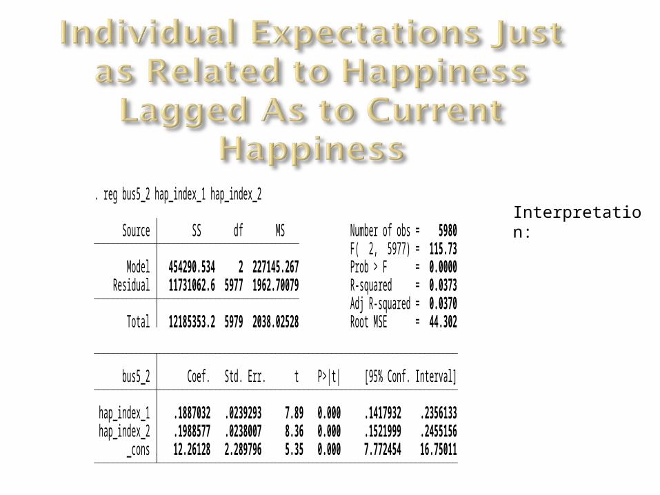
_cons 12.26128 2.289796 5.35 0.000 7.772454 16.75011 hap_index_2 .1988577 .0238007 8.36 0.000 .1521999 .2455156 hap_index_1 .1887032 .0239293 7.89 0.000 .1417932 .2356133 bus5_2 Coef. Std. Err. t P>|t| [95% Conf. Interval]

Total 12185353.2 5979 2038.02528 Root MSE = 44.302 Adj R-squared = 0.0370 Residual 11731062.6 5977 1962.70079 R-squared = 0.0373 Model 454290.534 2 227145.267 Prob > F = 0.0000 F( 2, 5977) = 115.73 Source SS df MS Number of obs = 5980

. reg bus5_2 hap_index_1 hap_index_2Interpretation:

Effect of household income on happiness

Table 2: Effect of Log Income on Happiness

Dependent Variable Regressor Effect size P-value

Happiness Average income over 6 mo. 0.226 0.000Change in income over 6 mo. 0.052 0.087

Change in happiness over 6 mo. Average income over 6 mo. -0.002 0.889Change in income over 6 mo. 0.069 0.038

To get intuition about the likely size of causal effects of changes in expectations on happiness at the 6 month frequency, let’s look at the effect of objective circumstances on happiness at the 6 month frequency.

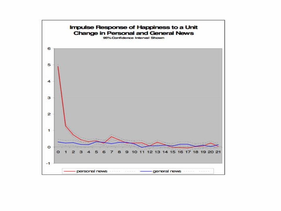
National News

Personal News

Econometric Issues for Later

• Discreteness of the components of the happiness index.

• Differential sensitivity of the components of the happiness index to the underlying latent variable.

• Plan: Use an approach similar to Kimball, Sahm and Shapiro, “Imputing Risk Tolerance from Survey Responses” JASA (forthcoming) and NBER 13337

Measurement Model

xitq xtN xi

P xitT si uit viq witq

xtN , xi

P , xitT , si ,ui ,vit ,witq orthogonal and i.i.d

xit1 HAPPY

xit 2 NOTSAD

xit 3 NOTDEPRESSED

xit 4 ENJOYLIFE

Component Impulse Responses (National News)

Impulse Response of Happiness Components to National News

-1.0

-0.5

0.0

0.5

1.0

1.5

2.0

-4 -3 -2 -1 0 1 2 3 4 5 6 7 8 9 10 11 12 13 14

Day

Co

effi

cien

t

"Feeling happy" "Not sad" "Feeling good" "Not depressed"

Component Impulse Responses (Personal News)

Impulse Response of Happiness Components to Personal News

-1.0

0.0

1.0

2.0

3.0

4.0

5.0

6.0

7.0

-4 -3 -2 -1 0 1 2 3 4 5 6 7 8 9 10 11 12 13 14

Day

Co

effi

cien

t

"Feeling happy" "Not sad" "Feeling good" "Not depressed

Measurement Modelxitq xt

N xiP xit

T si uit viq witq

LATENT HAPPINESS: xtN national,

xiP persistent personal, xit

T transitory personal.

IDIOSYNCRATIC RESPONSE ERROR:

si persistent, uit transitory,

ALL IDIOSYNCRATIC

QUESTION-SPECIFIC ELEMENTS:

viq persistent, witq transitory

Structural Model

yit N xtN Pxi

P T xitT ssi uuit it

yit Expectation or Evaluation

it uncorrelated with xiP , xit

T , si and uit for National y

(possibility of reverse causality yt xtN )

Structural Model: Comments

yit N xtN Pxi

P T xitT ssi uuit it

N : includes social construction of expectations

P : includes (1) habitual rose-colored glasses

(i.e., effects of personality-type) and

(2) effect of a good mood over extended time

T : effect of being in a good mood right now

s effect of persistent global response style

u effect of transitory global response style

Measurement Model for Happiness Index

xit xtN xi

P xitT si uit vi wit

where

xit (xit1 xit 2 xit 3 xit 4 ) / 4

vi (vi1 vi2 vi3 vi4 ) / 4

wit (wit1 wit 2 wit 3 wit 4 ) / 4

Measurement Model for Average Daily Happiness

Index of Othersx it xt

N x itP x it

T s it u it v it w it

where

x it x jt

jimt 1

etc.

NOTE: All components depend on the date because the set of “others” depends on the date.

Identifying N

Cov(xit , x it ) Cov(xtN xi

P xitT si uit vi wit ,

xtN x i

P x itT si u it v i w it )

Var(xtN )

Cov(yit , x it ) Cov( N xtN Pxi

P T xitT ssi uuit it ,

xtN x i

P x itT s i u it v i w it )

NVar(xtN ) Cov( it , xt

N )

(y x causation)

Identifying N

Cov(yit , xit )

Cov(xit , x it )N

Cov( it , xtN )

Var(xtN )

Persistence of national happiness

Estimated covariance of happiness with its own lags

-0.01

-0.005

0

0.005

0.01

0.015

0 5 10 15

Lag

Co

vari

ance

Covariance of happiness with lagged happiness

Persistence of national happiness

Table 5: Estimates of covariance of happiness with its own lags

Lag Covariance t-statistic 95% (low) 95% (high)0 0.0073531 2.3 0.0010768 0.01362931 0.0050124 2.18 0.0005042 0.00952072 0.0006685 0.28 -0.0040431 0.00538013 0.0061494 2.49 0.0013059 0.01099284 -0.0008634 -0.34 -0.0057708 0.0040445 -0.0002865 -0.11 -0.0053285 0.00475556 0.0007713 0.3 -0.0043453 0.00588797 -0.0034011 -1.3 -0.0085169 0.00171478 -0.0010418 -0.38 -0.006384 0.00430039 -0.0012532 -0.46 -0.0066251 0.0041187

10 -0.0027007 -0.95 -0.0082713 0.002869911 -0.0015549 -0.54 -0.0071569 0.00404712 -0.0008071 -0.28 -0.0064879 0.004873813 -0.0022994 -0.79 -0.0079699 0.003371114 0.0071094 2.44 0.001396 0.0128227

Effect of national happinessTable 6: Effect of national happiness on national expectation levels and vice versa

Variable Effect of happiness on variable P-value Effect of variable on happiness P-valuepago -0.350 0.430 -0.104 0.597pexp -0.864 0.175 -0.232 0.387bus12 0.325 0.625 0.135 0.201bus5 0.470 0.249 0.536 0.324dur 0.238 0.425 0.053 0.755inexq1 0.334 0.583 0.508 0.364v228 -0.093 0.889 0.567 0.179hom 0.047 0.946 124.249 0.995car 0.657 0.677 0.046 0.836homeval 0.284 0.691 -0.019 0.664bago 0.563 0.461 0.026 0.605bexp 0.765 0.078 0.085 0.739govt -0.341 0.629 0.215 0.731unemp 0.209 0.498 -0.260 0.454ratex 0.213 0.651 0.003 0.918gaspx1 -0.487 0.283 -0.513 0.104gas1px1 0.004 0.992 -0.016 0.849px1q1 0.081 0.859 0.258 0.217px5q1 -0.381 0.118 -0.476 0.395

Identifying P

Cov(yi2 , xi1 x i1) Cov( N x2N Pxi

P T xi2T ssi uui2 i2 ,

xiP x i1

P xi1T xi1

T (si ui1 vi wi1)

(s i1 u i1 v i1 w i1))

PVar(xiP ) sVar(si )

1=1st obs date, 2=2d obs date; cross-question covariance: rq

Cov(xi2q , xi1r x i1r ) Cov(xN xiP xi2

T (si ui2 viq wi2q ),

xiP x i1

P xi1T xi1

T (si ui1 vir wi1r ) (s i1 u i1 v i1r w i1r ))

Var(xiP ) Var(si )

Identifying P

Cov(yi2 , xi1 x i1)

Cov(xi2q , xi1r x i1r )(1 )P s ,

where =Var(si )

[Var(xiP ) Var(si )]

.

Identifying P

Cov(yi2 , xi1 x i1)

Cov(xi2q , xi1r x i1r )(1 )P s ,

where =Var(si )

[Var(xiP ) Var(si )]

.

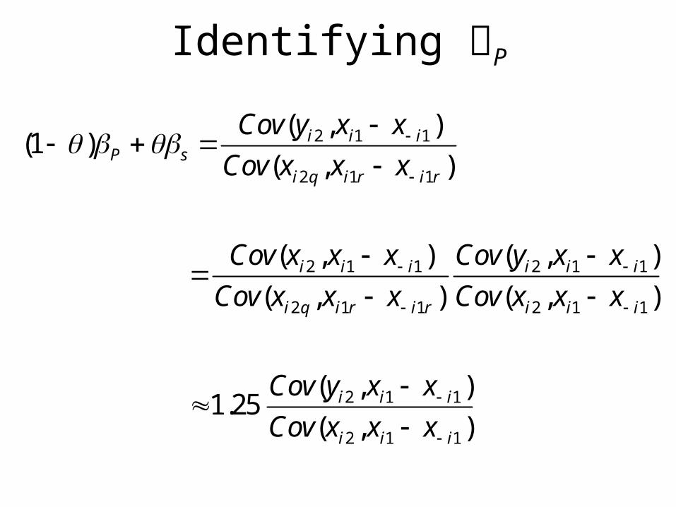
Identifying P

(1 )P s Cov(yi2 , xi1 x i1)

Cov(xi2q , xi1r x i1r )

Cov(xi2 , xi1 x i1)

Cov(xi2q , xi1r x i1r )Cov(yi2 , xi1 x i1)

Cov(xi2 , xi1 x i1)

1.25Cov(yi2 , xi1 x i1)

Cov(xi2 , xi1 x i1)

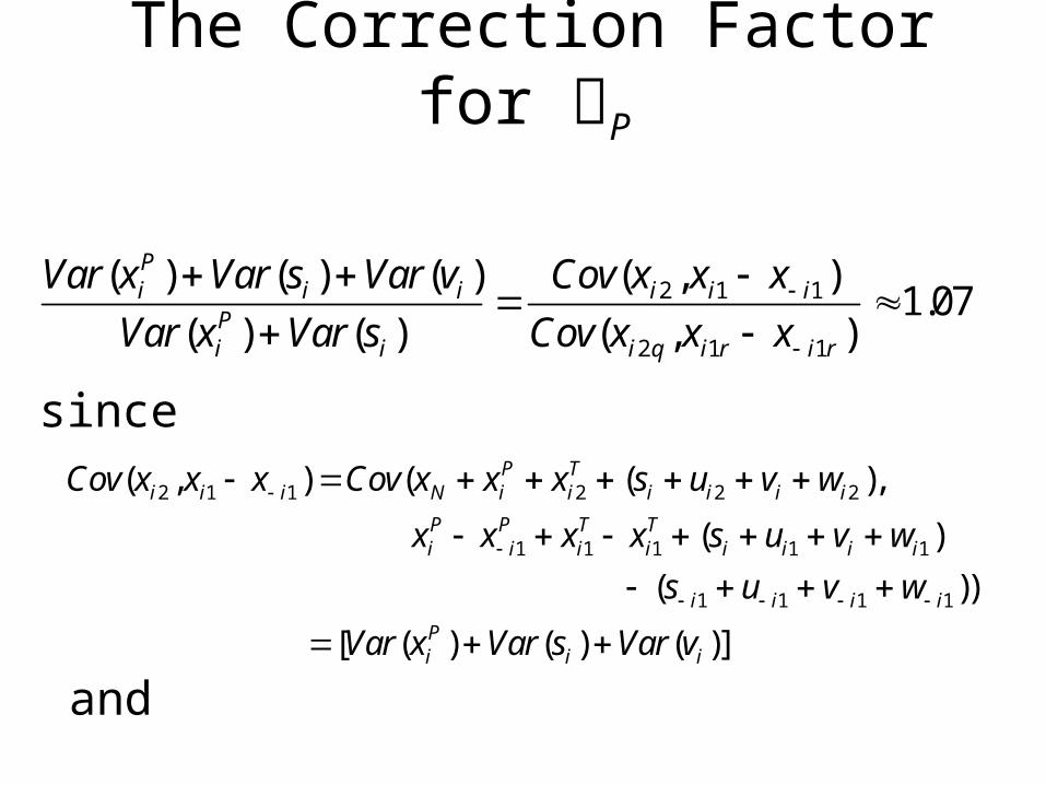
The Correction Factor for P

Var(xiP ) Var(si ) Var(vi )Var(xi

P ) Var(si )Cov(xi2 , xi1 x i1)

Cov(xi2q , xi1r x i1r )1.07

Cov(xi2 , xi1 x i1) Cov(xN xiP xi2

T (si ui2 vi wi2 ),

xiP x i1

P xi1T xi1

T (si ui1 vi wi1)

(s i1 u i1 v i1 w i1))

[Var(xiP ) Var(si ) Var(vi )]

since

and

Covariances of Happiness Responses across Contact Dates

[Average of All]/[Average off Diagonal] = 1.07

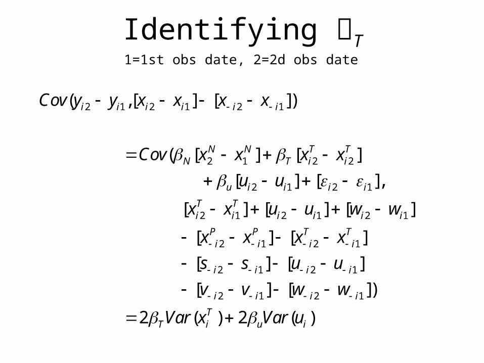
Identifying T

Cov(yi2 yi1,[xi2 xi1] [x i2 x i1])

Cov(N [x2N x1

N ] T [xi2T xi2

T ]

u[ui2 ui1] [ i2 i1],

[xi2T xi1

T ] [ui2 ui1] [wi2 wi1]

[x i2P x i1

P ] [x i2T x i1

T ]

[s i2 s i1] [u i2 u i1]

[v i2 v i1] [w i2 w i1])

2TVar(xiT ) 2uVar(ui )

1=1st obs date, 2=2d obs date

Identifying T

Cov(xi2q xi1q , [xi2r xi1r ] [x i2r x i1r ])

Cov([x2N x1

N ] [xi2T xi1

T ] [ui2 ui1] [wi2q wi1q ],

[xi2T xi1

T ] [ui2 ui1] [wi2r wi1r ]

[x i2P x i1

P ] [x i2T x i1

T ]

[s i2 s i1] [u i2 u i1]

[v i2r v i1r ] [w i2 w i1r ])

2[Var(xitT ) Var(uit )]

1=1st obs date, 2=2d obs date; cross-question covariance: rq

Identifying T

Cov(yi2 yi1, [xi2 xi1] [x i2 x i1])

Cov(xi2q xi1q , [xi2r xi1r ] [x i2r x i1r ])(1 )T u ,

where =Var(uit )

[Var(xitT ) Var(uit )]

.

Identifying T

(1 )T u Cov(yi2 yi1, [xi2 xi1] [x i2 x i1])

Cov(xi2q xi1q , [xi2r xi1r ] [x i2r x i1r ])

Cov(xi2 xi1, [xi2 xi1] [x i2 x i1])

Cov(xi2q xi1q , [xi2r xi1r ] [x i2r x i1r ])

Cov(yi2 yi1, [xi2 xi1] [x i2 x i1])

Cov(xi2 xi1, [xi2 xi1] [x i2 x i1])

1.91Cov(yi2 yi1, [xi2 xi1] [x i2 x i1])

Cov(xi2 xi1, [xi2 xi1] [x i2 x i1])

The Correction Factor for T

Var(xitT ) Var(uit ) Var(wit )Var(xit

T ) Var(uit )

Cov(xi2 xi1, [xi2 xi1] [x i2 x i1])

Cov(xi2q xi1q , [xi2r xi1r ] [x i2r x i1r ])

1.40

since

and

Cov(xi2 xi1, [xi2 xi1] [x i2 x i1])

Cov([x2N x1

N ] [xi2T xi1

T ] [ui2 ui1] [wi2 wi1],

[xi2T xi1

T ] [ui2 ui1] [wi2 wi1]

[x i2P x i1

P ] [x i2T x i1

T ]

[s i2 s i1] [u i2 u i1]

[v i2 v i1] [w i2 w i1])

2[Var(xitT ) Var(uit ) Var(wit )]

Covariances of 6-month changes in individual responses

to happiness questions

Average on Diagonal/Average off Diagonal = 1.400 (Omitting ENJOYLIFE: 1.421)

Bus5 (national, future, ρ=.446)“Which would you say is more likely – that in the country as a

whole we’ll have continuous good times during the next 5 years or so, or that we will have periods of widespread

unemployment and depression, or what?”

(1-)P s .521 (t=11.26)

(1 )T u=.05 (t=.014)

Bus12 (national, future, ρ=.422)“Do you think that during the next 12 months we’ll have good times financially, or bad times, or what?”

(1-)P s .393 (t=8.42)

(1 )T u=.050 (t=3.24)

P : includes (1) habitual rose-colored glasses

(i.e., effects of personality-type) and

(2) effect of a good mood over extended time

T : effect of being in a good mood right now

s effect of persistent global response style

u effect of transitory global response style

Why is (1 )T u so much smaller

than (1-)P s?

Sticky Expectations?

• People may not reevaluate their expectations every day.

• However, being interviewed may trigger the reevaluation of an expectations.

• If being interviewed does not trigger reevaluation, people can respond from explicit or implicit memory.

• Today’s happiness should only matter if the expectation is reevaluated, pushing down

T in relation to P .

Sticky Expectations: A Testable Prediction?

The ratio (1 )T u

(1-)P s should be smaller

for expectations and other judgments

that are likely to be reevaluted less often.

Bus5 (national, future, ρ=.446)“Which would you say is more likely – that in the country as a

whole we’ll have continuous good times during the next 5 years or so, or that we will have periods of widespread

unemployment and depression, or what?”

(1-)P s .521 (t=11.26)

(1 )T u=.05 (t=0.01)

Bus12 (national, future, ρ=.422)“Do you think that during the next 12 months we’ll have good times financially, or bad times, or what?”

(1-)P s .393 (t=8.42)

(1 )T u=.050 (t=3.24)

Px5q1 (national, future, ρ=.312)“Do you think prices will be higher, about the

same, or lower 5 to 10 years from now?”

(1-)P s .102 (t= 2.23)

(1 )T u=-.003 (t= 0.02)

Px1q1 (national, future, ρ=.263)“Do you think that during the next 12 months, prices will go up, or go down, or stay where they are now?”

(1-)P s .057 (t=1.26)

(1 )T u=.020 (t=1.25)

Gaspx1 (national, future, ρ=.318)“Do you think that the price of gasoline will go up during the next 5 years, go down, or stay

about the same?”

(1-)P s .032 (t=0.75)

(1 )T u=.004 (t=0.27)

Gas1px1 (national, future, ρ=.231)“Do you think that the price of gasoline will go up during the next 12 months, go down, or stay about the same?”

(1-)P s .029 (t=0.65)

(1 )T u=.015 (t=0.85)

Bexp (national, future, ρ=.323)“A year from now, do you expect that in the country as a whole business conditions will be better, or worse than

they are at present, or just about the same?”

(1-)P s .145 (t=4.27)

(1 )T u=.005 (t=0.23)

Ratex (national, future, ρ=.297)“What do you think will happen to interest rates for borrowing money over the next 12 months – will they go up, stay the same, or go down?”

(1-)P s .145 (t=4.02)

(1 )T u=.015 (t=0.69)

Unemp (national, future, ρ=.285)“How about people out of work during the

coming 12 months – do you think that there will be more unemployment than now, about the

same, or less?”

(1-)P s .132 (t=3.93)

(1 )T u=.057 (t=2.71)Dur (national, present, ρ=.274)“Generally speaking, do you think now is a good time or a bad time for people to buy major household items?”

(1-)P s .148 (t=4.11)

(1 )T u=.050 (t=2.22)

Govt (national, present, ρ=.539)“As to the economic policy of the government – I mean steps taken to fight inflation or unemployment – would you say the

government is doing a good job, only fair, or a poor job?”

(1-)P s .338 (t=9.91)

(1 )T u=.049 (t=2.89)

Bago (national, past, ρ=.345)“Would you say that at the present time business conditions are better or worse than they were a year ago?”

(1-)P s .155 (t=4.64)

(1 )T u=.036 (t=1.77)

Conclusions: General

1. The variance and persistence of national happiness are small.

2. Happiness affects expectations causally.

3. Suggestive evidence for sticky expectations- expectations that people would plausibly

reevaluate less often seem less affected by changes in happiness.

Conclusions: Animal Spirits vs. Information

• Upper bound on the size of business cycle fluctuations that are caused by structural shocks to the emotion of happiness.

• Bad for the “animal spirits” view• Happiness does seem to affect expectations,

but happiness is mostly idiosyncratic. • Leaves plenty of room for the empirical

successes of the information view based on aggregate data.

Inexq1 (personal, future, ρ=.416)“During the next 12 months, do you expect your

(family) income to be higher or lower than during the past year?”

(1-)P s .176 (t=5.17)

(1 )T u=.067 (t=3.54)Pexp (personal, future, ρ=.419)“Do you think that a year from now you (and your family living there) will be better off financially, or worse off, or just about the same as now?”

(1-)P s .124 (t=3.67)

(1 )T u=.013 (t=0.70)

Pago (personal, past, ρ=.462)“Would you say that you (and your family living there) are better off or worse off financially than a year ago?”

(1-)P s .402 (t=11.87)

(1 )T u=.047 (t=2.60)

V228 (personal, past, ρ=.429)“Compared with 5 years ago, do you think the chances that you (and your husband/wife) will have a comfortable retirement have gone up, gone down, or remained about the same?”

(1-)P s .275 (t=8.22)

(1 )T u=.084 (t=4.51)

Homeval (personal, past, ρ=.580)“Do you think the present value of your home – I mean

what it would bring you if you sold it today – has increased compared with a year ago, decreased, or

stayed about the same?”

(1-)P s .090 (t=2.14)

(1 )T u=.013 (t=.069)

Hom (personal, present, ρ=.361)“Generally speaking, do you think now is a good time or a bad time to buy a house?”

(1-)P s .247 (t=7.22)

(1 )T u= .001 (t= 0.03)

Car (personal, future, ρ=.286)“Do you think the next 12 months will be a good

time or a bad time to buy a vehicle?”

(1-)P s .208 (t=5.81)

(1 )T u=.000 (t=0.00)