BMEGUI Tutorial 3 Space/time BME for synchronized data

1. Objective

The primary objective of this tutorial is to perform the full space/time BME analysis on a

simulated dataset where all the measurements are collected at fixed monitoring sites, and

synchronized times. The analysis will consist in an exploratory analysis of the data across

space and time, in the modeling of its global space/time mean trend and space/time

covariance, and in obtaining plots showing the BME estimate as a function of time, as

well as maps of the BME estimates across space.

2. Install BMEGUI 3.0.1

See tutorial 1.

3. Data

Download the data file “data03.csv” from the Tutorial Data Files and save it in a folder

called “work03”. Open the data file using a spreadsheet editor or a text editor to see the

data available. Note that there are 15 measurements collected at 15 different spatial

locations at time 1, followed by 15 measurements collected at the same spatial locations

at time 2, 3, 4, 5, 6, 7, 8, 9, and 10.

4. Operation

i. Launch BMEGUI by double clicking on ‘BMEGUI’ desktop icon. Refer to the

BMEGUI 3.0.1 user’s manual for more details.

ii. Run the BMEGUI tool and select the following workspace and data file.

Workspace: work03

Data File: data03.csv

Figure 1: Data and directory selection BMGUI screen

iii. Click on the “OK” button. The “Data Field” screen appears.

iv. In the “Data Field Setting” section, check the “Use Datatype” button and select

the following column names from the dropdown menu in each field.

X Field: X

Y Field: Y

Time Field: T

ID: Automatic ID

Data Type: Type

Value1 Field: Val1

Value2 Field: Val2

Value3 Field: Val3

Value4 Field: Val4

v. In the “Unit/Name” section, input the following units and name of data in each

entry box.

Space Unit: deg.

Time Unit: days

Data Unit: ug/L

Name of Data: Contaminant C

Figure 2: The “Data Field” screen

vi. Click on the “Next” button. The “Data Distribution” screen appears

vii. Check the basic statistics (mean, standard deviation, coefficient of skewness, and

coefficient of kurtosis) of the data and its log-transformed data in the “Statistics”

section.

viii. Check the histograms of raw data and log-transformed data. By clicking the “Raw

Data” and “Log Data” tab in the “Histogram” section, you can switch the

histograms

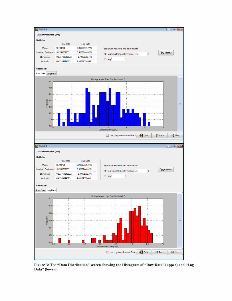
Figure 3: The “Data Distribution” screen showing the Histogram of “Raw Data” (upper) and “Log

Data” (lower)

ix. Click on the “Next” button. The “Exploratory Data Analysis” screen appears

x. Click on the “Temporal Evolution” tab. Change the “Station ID” and see the

corresponding temporal distribution of the data

xi. Click on the “Spatial Distribution” tab. Change the “Time” and see the

corresponding spatial distribution of the data

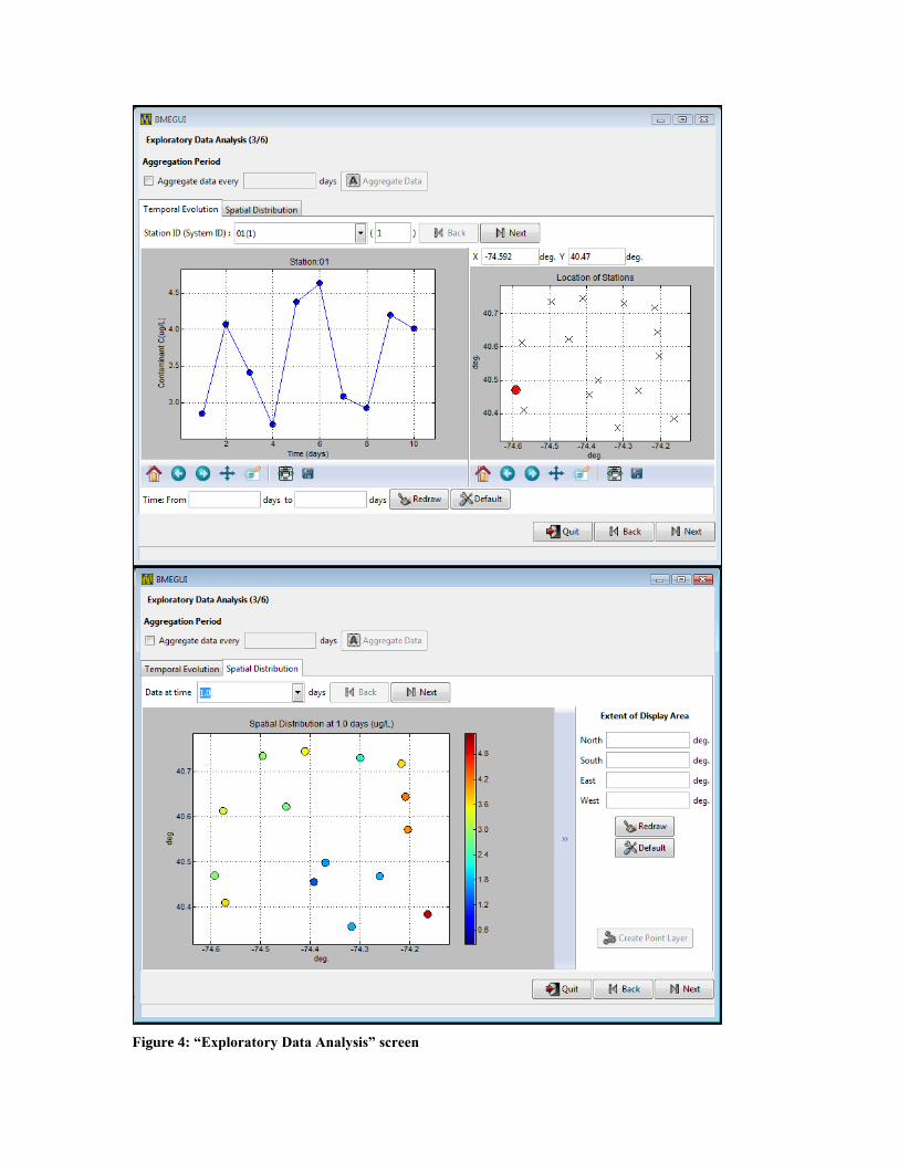
Figure 4: “Exploratory Data Analysis” screen

xii. Click on the “Next” button. The “Mean Trend Analysis” screen appears

xiii. Click on the “Model mean trend and remove it from data” button to plot the mean

trend

xiv. To obtain the mean trend using new parameters, input the following parameter

values, and click on the “Recalculate Mean Trend” button

Search Radius Smoothing Range

Spatial 1 0.12

Temporal 10 2

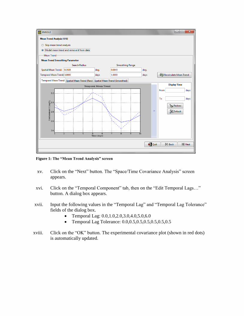
Figure 1: The “Mean Trend Analysis” screen

xv. Click on the “Next” button. The “Space/Time Covariance Analysis” screen

appears.

xvi. Click on the “Temporal Component” tab, then on the “Edit Temporal Lags…”

button. A dialog box appears.

xvii. Input the following values in the “Temporal Lag” and “Temporal Lag Tolerance”

fields of the dialog box.

Temporal Lag: 0.0,1.0,2.0,3.0,4.0,5.0,6.0

Temporal Lag Tolerance: 0.0,0.5,0.5,0.5,0.5,0.5,0.5

xviii. Click on the “OK” button. The experimental covariance plot (shown in red dots)

is automatically updated.

Figure 2: The “Space/Time Covariance Analysis” screen, showing Temporal Component of the

covariance

xix. Input the following model parameters

Sill: 0.80122

Spatial Model: exponentialC

Spatial Range: 0.16

Temporal Model: exponentialC

Temporal Range: 5

xx. Click on the “Plot Model” button. A plot of covariance model is superimposed on

the experimental covariance values.

Figure 3: The covariance model, shown on the Spatial Component (upper) and Temporal

Component (lower) plot

NOTE: alternatively you can also fit covariance model by clicking on ‘Automatic Cov

Fit’ button.

xxi. Click on the “Next” button. The “BME Estimation” screen appears.

xxii. Click on the “Spatial Distribution” tab. To obtain the BME estimation at 5.0 (day),

use following parameters

BME Parameters: Use default

Estimation Grid:

Estimation Time: 5.0

Check “Include Data Points”

Check “Include Voronoi Points”

Display Grid: Use default

xxiii. Click on the “Estimate” button. Two new tabs labeled “Plot ID: 0001(Mean)” and

“Plot ID: 0001(Error)” appear, and a new entry appears on the list in the “Maps

Estimated” section.

Figure 4: The “BME Estimation” screen

xxiv. Click on the “Plot ID: 0001(Mean)” tab and check the map of BME mean

estimates.

xxv. Click on the “Plot ID: 0001(Error)” tab and check the map of BME error variance.

Figure 5: Maps of the BME mean estimate and BME error variance

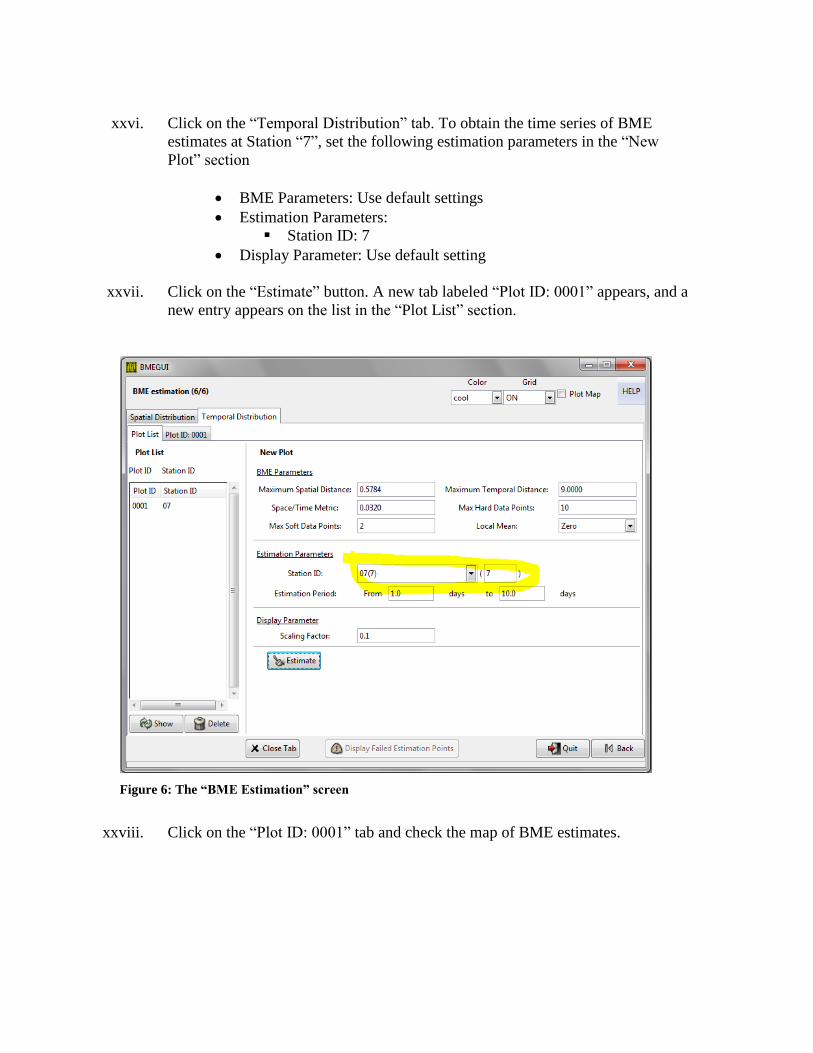
xxvi. Click on the “Temporal Distribution” tab. To obtain the time series of BME

estimates at Station “7”, set the following estimation parameters in the “New

Plot” section

BME Parameters: Use default settings

Estimation Parameters:

Station ID: 7

Display Parameter: Use default setting

xxvii. Click on the “Estimate” button. A new tab labeled “Plot ID: 0001” appears, and a

new entry appears on the list in the “Plot List” section.

Figure 6: The “BME Estimation” screen

xxviii. Click on the “Plot ID: 0001” tab and check the map of BME estimates.

Figure 7: Time series of BME estimates

xxix. Click on the “Quit” button to close the screen. A dialog box appears. Click on the

“OK” button of that dialog box to confirm that you want to quit BMEGUI.