BlueScout 1 Wind Measurements and Power

© BlueScout Technologies, Inc. www.BlueScout.com

1

Wind Measurements and Power

A great wind is blowing, and that gives you

either imagination or a headache.

Catherine the Great (1729-1796)

Introduction The wind is a curious creature, blowing this way and that. Mathematicians would say that wind is a classic example of chaos. If asked about the wind, a surfer would simply shrug and say that waves are crazy, too. This powerful, but also quirky creature, the breeze that makes a child smile- this is what we must capture. Our world needs us, the wind turbine industry, to produce power, cleanly, efficiently and at low cost. Here at BlueScout, our contribution to the wind industry is to use our understanding of optics to provide a fundamentally deeper understanding of the wind resource - to produce substantial, repeatable increases in the output power of wind turbines.

Synopsis A BlueScout Optical Control System (OCS), beta-version, is tested upon an operating utility scale wind turbine. The turbine was operated in four regimes; legacy yaw control (sonic anemometer) and three OCS control regimes. The behavior of the sonic anemometer, measuring both speed and wind angle, is studied. The uptime of the OCS is studied. Power curves in the four regimes are compared.

Data Set and Analytic Tools The data set is large, approximately 500 MB, composed of 335,000 data points taken at 1 second spacing. SAS JMP used as the statistical analytic tool. The dataset includes output from the OCS, two sonic anemometers (giving both wind speed and wind direction), turbine state, ambient temperature, output power, and absolute yaw position.


2

The Ideal Wind Turbine Wind has a mind of its own; it is turbulent, has shear, changes direction, and changes velocity. An ideal wind turbine needs to be pointed in the right direction, with its blades set at the correct angle to the wind. When a gust approaches, an ideal turbine will take actions to avoid damage. Practically, this means that the turbine has sufficient wind data to properly adjust blade pitch and yaw, is equipped with adjustable pitch and yaw, and has a control architecture that is sufficiently sophisticated to translate wind data into the appropriate turbine actions. To properly adjust the pitch of all of the blades at the same time (“collective” pitch control) requires an accurate understanding of the average wind speed approaching the entire spatial plane of the blades of the turbine. To properly adjust the pitch of each blade individually (“individual” pitch control) requires both rapid pitch adjustment and an accurate mapping of the variance (either modeled or measured directly) of the wind speed incident upon the turbine. A discussion of 2-D mapping is outside of the scope of this discussion. Correct yaw adjustment implies that the turbine understands the direction of the wind, as it approaches the blades of the turbine. As an aside, we note that most analysis of a wind turbine, particular work on advanced control algorithms and controller analysis and design tend to begin with an a priori assumption that the there is no yaw misalignment. The data collected in this work, regardless of which control algorithm is used, clearly demonstrated that the assumption of no yaw misalignment is not valid. Gust avoidance is possible when the turbine knows the wind speed and direction that will hit the wind turbine, with enough warning time to take actions to avoid damage.

Current State of the Art

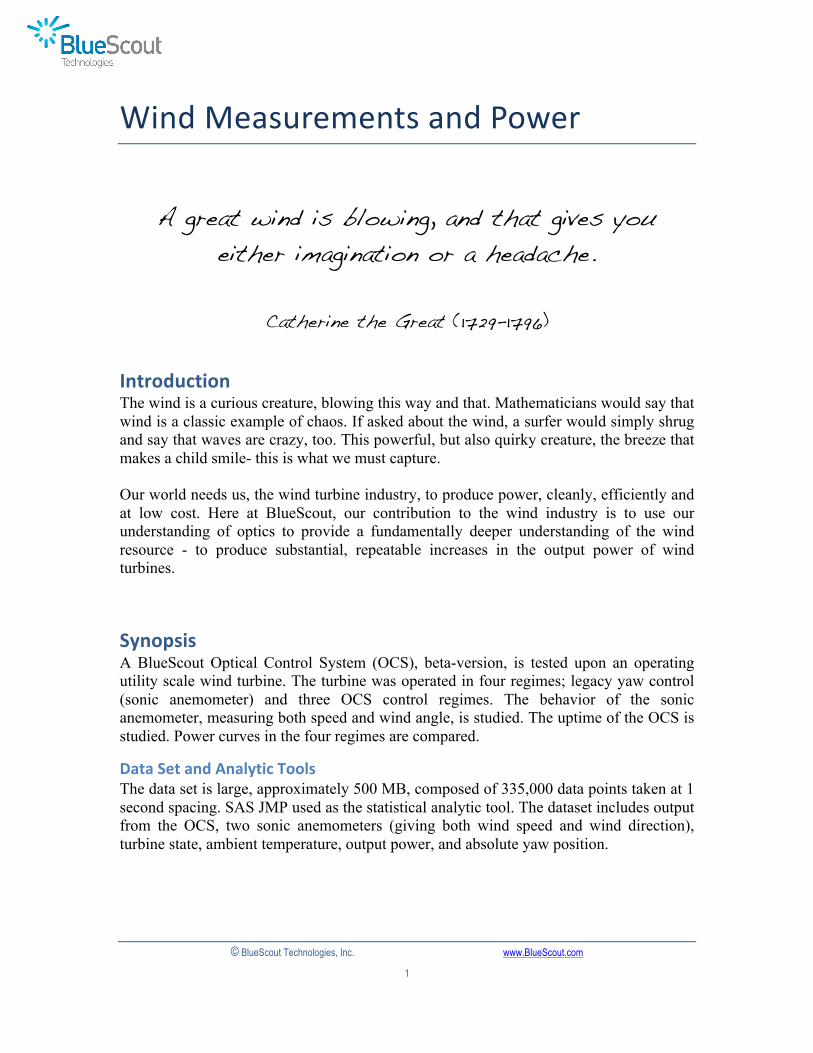
Speed Measurement Wind turbines today use anemometers, mounted on the rear of the nacelle, to measure wind speed. Although these are high quality wind measurement devices, they cannot be mounted in front of the turbine and, hence, must operate in the turbulent air that has already passed through the turbine blades, which has little resemblance to the wind condition in front of the blades. Figure 1 shows the raw output of a sonic anemometer in action. The horizontal axis is recorded seconds, with the figure capturing 10 minutes of operation. This particular turbine model has two sonic anemometers; Figure 1 only shows the output of one of the two sonic anemometers. Throughout this document, the sonic anemometers are referred to as A1 and A2.


3

Figure 1 The data of a sonic anemometer, mounted on the rear of the nacelle of an operating wind turbine. The data is taken each second of operation. The period shown here covers a 10 minute interval.

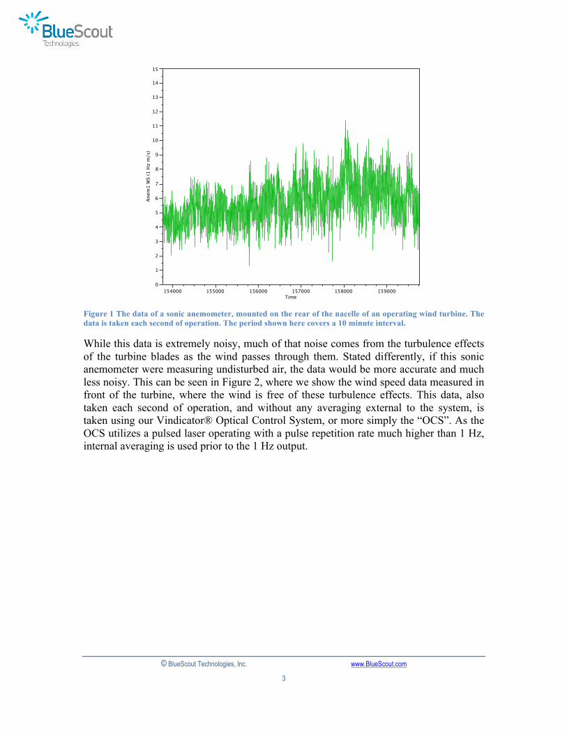
While this data is extremely noisy, much of that noise comes from the turbulence effects of the turbine blades as the wind passes through them. Stated differently, if this sonic anemometer were measuring undisturbed air, the data would be more accurate and much less noisy. This can be seen in Figure 2, where we show the wind speed data measured in front of the turbine, where the wind is free of these turbulence effects. This data, also taken each second of operation, and without any averaging external to the system, is taken using our Vindicator® Optical Control System, or more simply the “OCS”. As the OCS utilizes a pulsed laser operating with a pulse repetition rate much higher than 1 Hz, internal averaging is used prior to the 1 Hz output.

Nordex_active: Overlay Plot by Time Page 2 of 5154000 155000 156000 157000 158000 159000

Time

0

1

2

3

4

5

6

7

8

9

10

11

12

13

14

15

Ane

m1

WS

(1 H

z m

/s)

154000 155000 156000 157000 158000 159000Time

Overlay Plot


4

Figure 2 The wind speed in front of the turbine, measured with the OCS.This data is also taken each second, un-averaged, with a 10-minute period of operation shown.

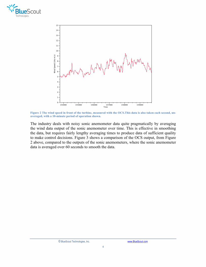
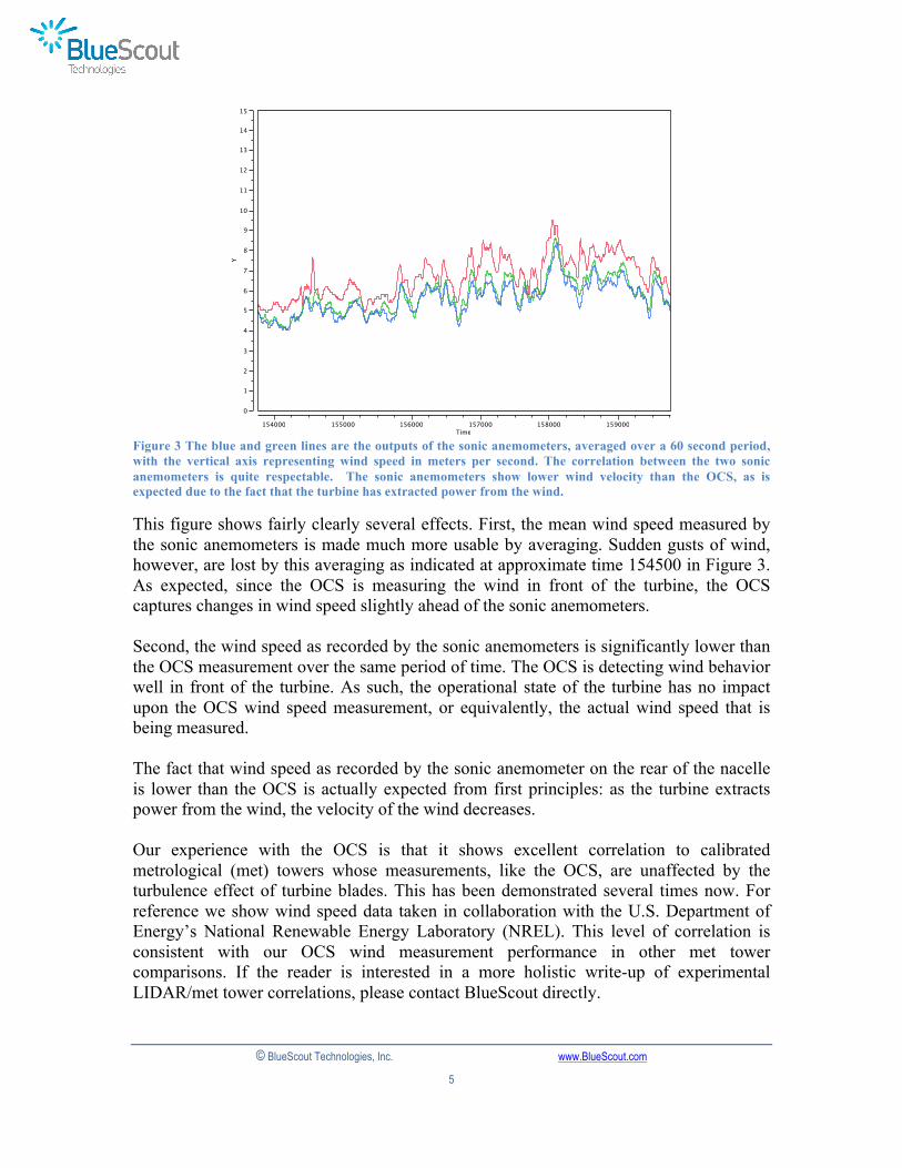
The industry deals with noisy sonic anemometer data quite pragmatically by averaging the wind data output of the sonic anemometer over time. This is effective in smoothing the data, but requires fairly lengthy averaging times to produce data of sufficient quality to make control decisions. Figure 3 shows a comparison of the OCS output, from Figure 2 above, compared to the outputs of the sonic anemometers, where the sonic anemometer data is averaged over 60 seconds to smooth the data.

Nordex_active: Overlay Plot by Time Page 1 of 5

0

1

2

3

4

5

6

7

8

9

10

11

12

13

14

15

Win

d Sp

eed

(1H

z m

/s)

154000 155000 156000 157000 158000 159000Time

Overlay Plot


5

Figure 3 The blue and green lines are the outputs of the sonic anemometers, averaged over a 60 second period, with the vertical axis representing wind speed in meters per second. The correlation between the two sonic anemometers is quite respectable. The sonic anemometers show lower wind velocity than the OCS, as is expected due to the fact that the turbine has extracted power from the wind.

This figure shows fairly clearly several effects. First, the mean wind speed measured by the sonic anemometers is made much more usable by averaging. Sudden gusts of wind, however, are lost by this averaging as indicated at approximate time 154500 in Figure 3. As expected, since the OCS is measuring the wind in front of the turbine, the OCS captures changes in wind speed slightly ahead of the sonic anemometers. Second, the wind speed as recorded by the sonic anemometers is significantly lower than the OCS measurement over the same period of time. The OCS is detecting wind behavior well in front of the turbine. As such, the operational state of the turbine has no impact upon the OCS wind speed measurement, or equivalently, the actual wind speed that is being measured. The fact that wind speed as recorded by the sonic anemometer on the rear of the nacelle is lower than the OCS is actually expected from first principles: as the turbine extracts power from the wind, the velocity of the wind decreases. Our experience with the OCS is that it shows excellent correlation to calibrated metrological (met) towers whose measurements, like the OCS, are unaffected by the turbulence effect of turbine blades. This has been demonstrated several times now. For reference we show wind speed data taken in collaboration with the U.S. Department of Energy’s National Renewable Energy Laboratory (NREL). This level of correlation is consistent with our OCS wind measurement performance in other met tower comparisons. If the reader is interested in a more holistic write-up of experimental LIDAR/met tower correlations, please contact BlueScout directly.


0

1

2

3

4

5

6

7

8

9

10

11

12

13

14

15

Y

154000 155000 156000 157000 158000 159000Time

Overlay Plot

Y Wind Speed (1Hz m/s) 30 Sec Avg Anem1 WS 30 Sec Avg Anem2 WS


6

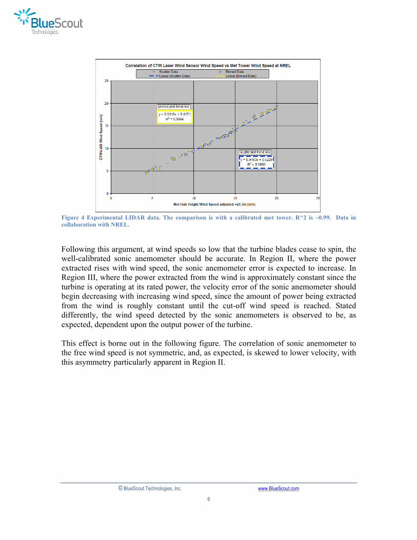
Figure 4 Experimental LIDAR data. The comparison is with a calibrated met tower. R^2 is ~0.99. Data in collaboration with NREL.

Following this argument, at wind speeds so low that the turbine blades cease to spin, the well-calibrated sonic anemometer should be accurate. In Region II, where the power extracted rises with wind speed, the sonic anemometer error is expected to increase. In Region III, where the power extracted from the wind is approximately constant since the turbine is operating at its rated power, the velocity error of the sonic anemometer should begin decreasing with increasing wind speed, since the amount of power being extracted from the wind is roughly constant until the cut-off wind speed is reached. Stated differently, the wind speed detected by the sonic anemometers is observed to be, as expected, dependent upon the output power of the turbine. This effect is borne out in the following figure. The correlation of sonic anemometer to the free wind speed is not symmetric, and, as expected, is skewed to lower velocity, with this asymmetry particularly apparent in Region II.


7

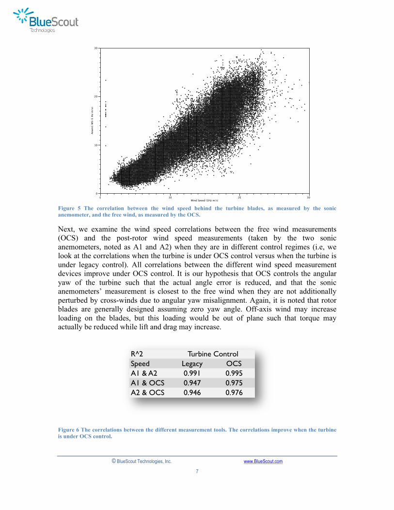
Figure 5 The correlation between the wind speed behind the turbine blades, as measured by the sonic anemometer, and the free wind, as measured by the OCS.

Next, we examine the wind speed correlations between the free wind measurements (OCS) and the post-rotor wind speed measurements (taken by the two sonic anemometers, noted as A1 and A2) when they are in different control regimes (i.e, we look at the correlations when the turbine is under OCS control versus when the turbine is under legacy control). All correlations between the different wind speed measurement devices improve under OCS control. It is our hypothesis that OCS controls the angular yaw of the turbine such that the actual angle error is reduced, and that the sonic anemometers’ measurement is closest to the free wind when they are not additionally perturbed by cross-winds due to angular yaw misalignment. Again, it is noted that rotor blades are generally designed assuming zero yaw angle. Off-axis wind may increase loading on the blades, but this loading would be out of plane such that torque may actually be reduced while lift and drag may increase.

Figure 6 The correlations between the different measurement tools. The correlations improve when the turbine is under OCS control.

Nordex Data: Overlay Plot Page 1 of 3

0

10

20

30

Ane

m1

WS

(1 H

z m

/s)

0 10 20 30Wind Speed (1Hz m/s)

Overlay Plot Control (0-legacy 1-Vind)=0

Overlay Plot Control (0-legacy 1-Vind)=1

R^2Speed Legacy OCSA1 & A2 0.991 0.995A1 & OCS 0.947 0.975A2 & OCS 0.946 0.976

Turbine Control


8

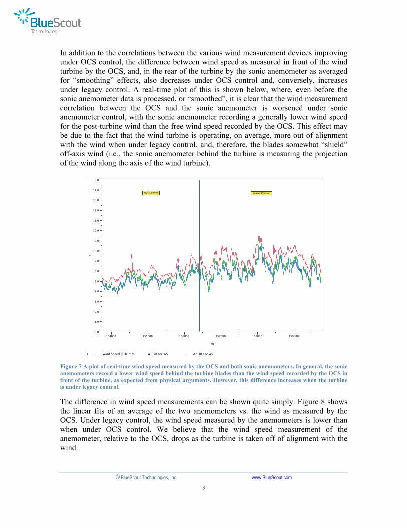
In addition to the correlations between the various wind measurement devices improving under OCS control, the difference between wind speed as measured in front of the wind turbine by the OCS, and, in the rear of the turbine by the sonic anemometer as averaged for “smoothing” effects, also decreases under OCS control and, conversely, increases under legacy control. A real-time plot of this is shown below, where, even before the sonic anemometer data is processed, or “smoothed”, it is clear that the wind measurement correlation between the OCS and the sonic anemometer is worsened under sonic anemometer control, with the sonic anemometer recording a generally lower wind speed for the post-turbine wind than the free wind speed recorded by the OCS. This effect may be due to the fact that the wind turbine is operating, on average, more out of alignment with the wind when under legacy control, and, therefore, the blades somewhat “shield” off-axis wind (i.e., the sonic anemometer behind the turbine is measuring the projection of the wind along the axis of the wind turbine).

Figure 7 A plot of real-time wind speed measured by the OCS and both sonic anemometers. In general, the sonic anemometers record a lower wind speed behind the turbine blades than the wind speed recorded by the OCS in front of the turbine, as expected from physical arguments. However, this difference increases when the turbine is under legacy control.

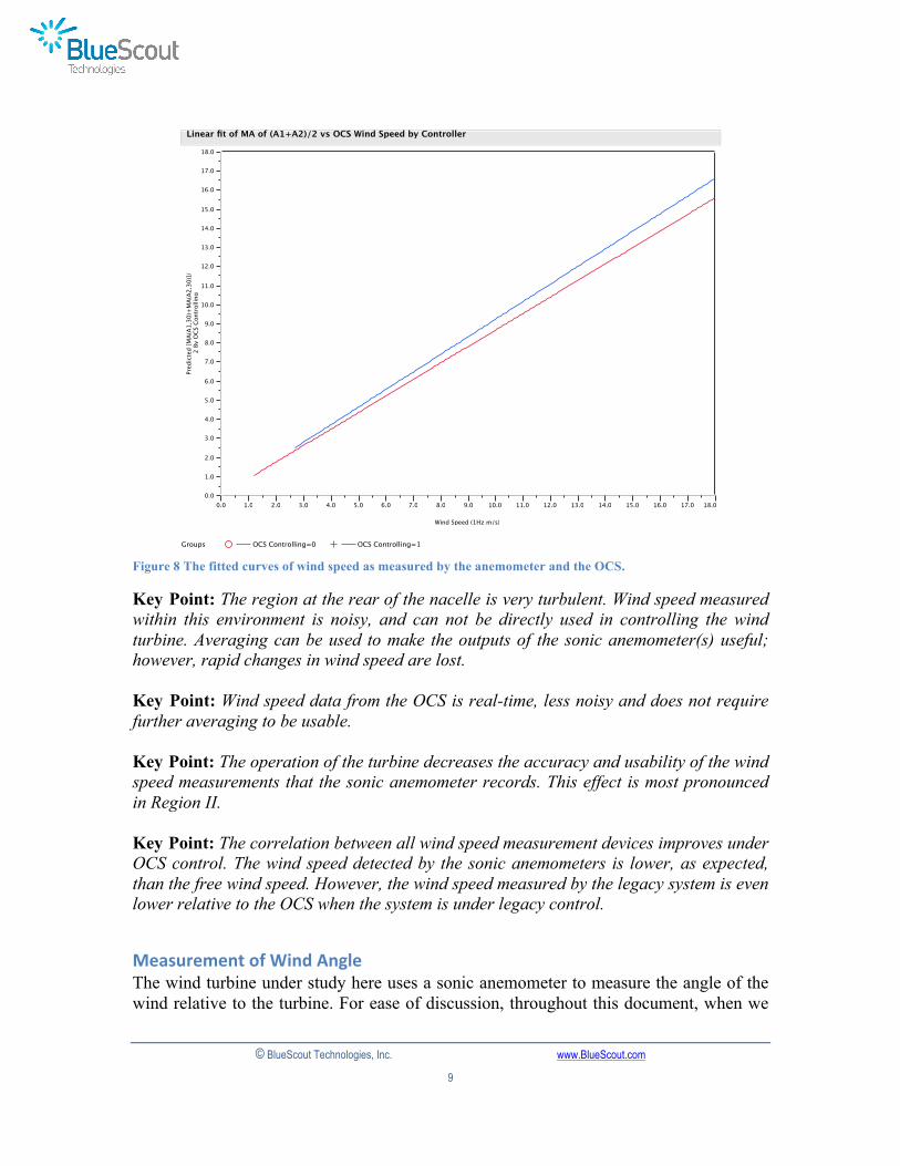
The difference in wind speed measurements can be shown quite simply. Figure 8 shows the linear fits of an average of the two anemometers vs. the wind as measured by the OCS. Under legacy control, the wind speed measured by the anemometers is lower than when under OCS control. We believe that the wind speed measurement of the anemometer, relative to the OCS, drops as the turbine is taken off of alignment with the wind.

Nordex_Turbine_OCS_online_turbine_time: Overlay Plot by Time Page 1 of 1

0.0

1.0

2.0

3.0

4.0

5.0

6.0

7.0

8.0

9.0

10.0

11.0

12.0

13.0

14.0

15.0

Y

154000 155000 156000 157000 158000 159000

Time

OCS WS, 30 sec MA of A1, A2 WS

OCS Control Legacy Control

Y Wind Speed (1Hz m/s) A1 30 sec WS A2 30 sec WS


9

Figure 8 The fitted curves of wind speed as measured by the anemometer and the OCS.

Key Point: The region at the rear of the nacelle is very turbulent. Wind speed measured within this environment is noisy, and can not be directly used in controlling the wind turbine. Averaging can be used to make the outputs of the sonic anemometer(s) useful; however, rapid changes in wind speed are lost. Key Point: Wind speed data from the OCS is real-time, less noisy and does not require further averaging to be usable. Key Point: The operation of the turbine decreases the accuracy and usability of the wind speed measurements that the sonic anemometer records. This effect is most pronounced in Region II. Key Point: The correlation between all wind speed measurement devices improves under OCS control. The wind speed detected by the sonic anemometers is lower, as expected, than the free wind speed. However, the wind speed measured by the legacy system is even lower relative to the OCS when the system is under legacy control.

Measurement of Wind Angle The wind turbine under study here uses a sonic anemometer to measure the angle of the wind relative to the turbine. For ease of discussion, throughout this document, when we

Nordex_Turbine_OSC_online: Overlay Plot of Predicted [MA(A1,30)+MA(A2,30)]/2 By OCS Controlling by Wind Speed (1Hz m/s) Page 1 of 1

0.0

1.0

2.0

3.0

4.0

5.0

6.0

7.0

8.0

9.0

10.0

11.0

12.0

13.0

14.0

15.0

16.0

17.0

18.0

Pred

icte

d [M

A(A1

,30)

+M

A(A2

,30)

]/2

By O

CS C

ontr

ollin

g

0.0 1.0 2.0 3.0 4.0 5.0 6.0 7.0 8.0 9.0 10.0 11.0 12.0 13.0 14.0 15.0 16.0 17.0 18.0

Wind Speed (1Hz m/s)

Linear fit of MA of (A1+A2)/2 vs OCS Wind Speed by Controller

Groups OCS Controlling=0 OCS Controlling=1


10

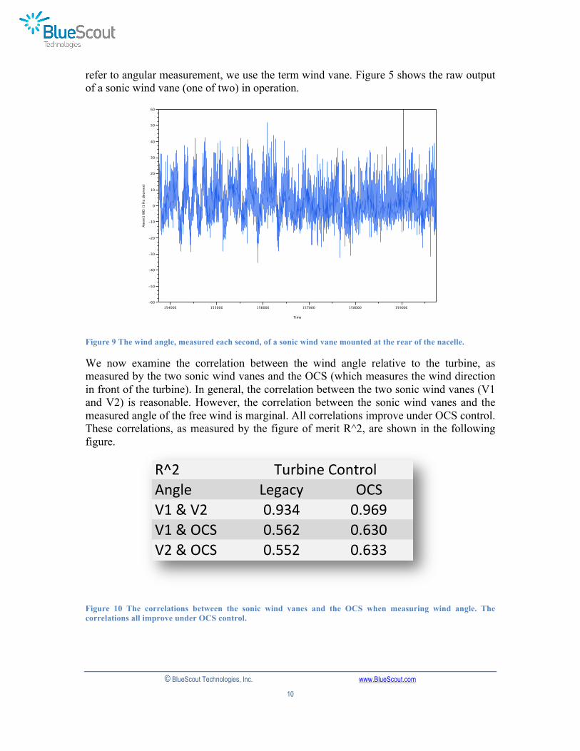
refer to angular measurement, we use the term wind vane. Figure 5 shows the raw output of a sonic wind vane (one of two) in operation.

Figure 9 The wind angle, measured each second, of a sonic wind vane mounted at the rear of the nacelle.

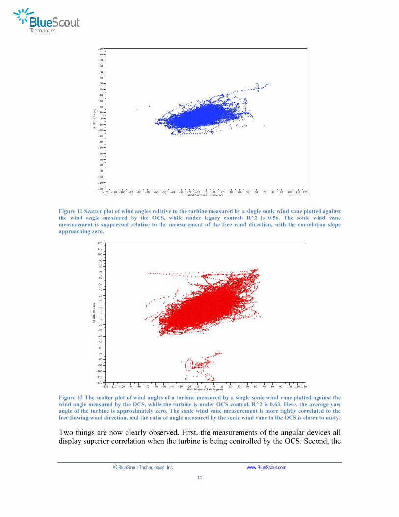
We now examine the correlation between the wind angle relative to the turbine, as measured by the two sonic wind vanes and the OCS (which measures the wind direction in front of the turbine). In general, the correlation between the two sonic wind vanes (V1 and V2) is reasonable. However, the correlation between the sonic wind vanes and the measured angle of the free wind is marginal. All correlations improve under OCS control. These correlations, as measured by the figure of merit R^2, are shown in the following figure.

Figure 10 The correlations between the sonic wind vanes and the OCS when measuring wind angle. The correlations all improve under OCS control.

Nordex_Turbine_OSC_online: Overlay Plot of Anem1 WD (1 Hz degrees) by Time Page 1 of 1

-60

-50

-40

-30

-20

-10

0

10

20

30

40

50

60

Ane

m1

WD

(1 H

z de

gree

s)

154000 155000 156000 157000 158000 159000

Time

A1 Wind Direction (no averaging) vs. Time - 10 min. window

R^2Angle) Legacy OCSV1)&)V2 0.934 0.969V1)&)OCS 0.562 0.630V2)&)OCS 0.552 0.633

Turbine)Control


11

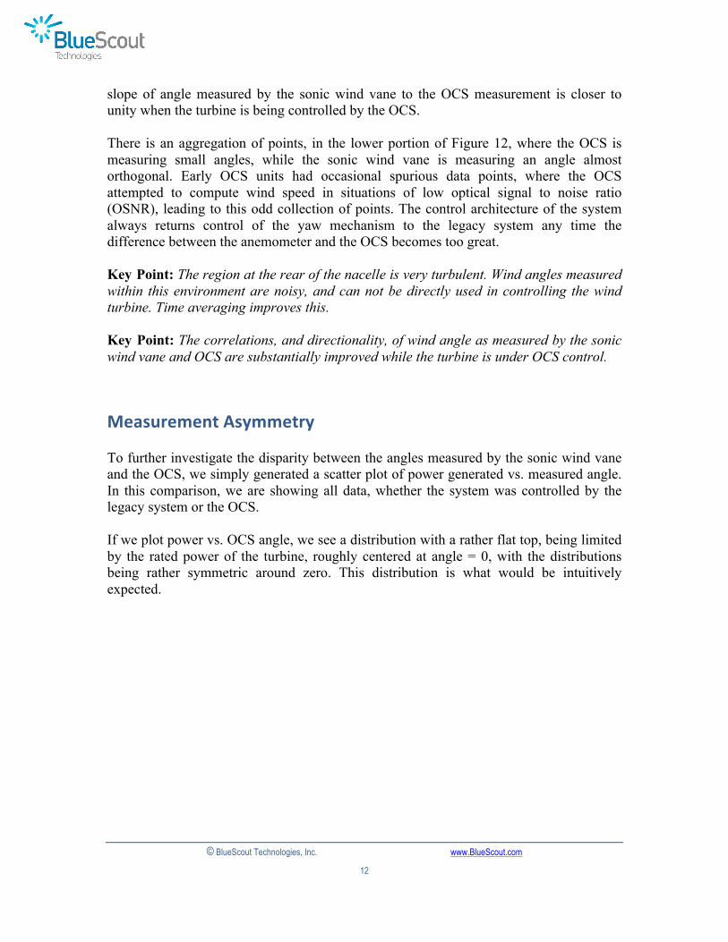
Figure 11 Scatter plot of wind angles relative to the turbine measured by a single sonic wind vane plotted against the wind angle measured by the OCS, while under legacy control. R^2 is 0.56. The sonic wind vane measurement is suppressed relative to the measurement of the free wind direction, with the correlation slope approaching zero.

Figure 12 The scatter plot of wind angles of a turbine measured by a single sonic wind vane plotted against the wind angle measured by the OCS, while the turbine is under OCS control. R^2 is 0.63. Here, the average yaw angle of the turbine is approximately zero. The sonic wind vane measurement is more tightly correlated to the free flowing wind direction, and the ratio of angle measured by the sonic wind vane to the OCS is closer to unity.

Two things are now clearly observed. First, the measurements of the angular devices all display superior correlation when the turbine is being controlled by the OCS. Second, the

Nordex_Turbine_OSC_online: Overlay Plot Page 1 of 2

-120

-110

-100

-90

-80

-70

-60

-50

-40

-30

-20

-10

0

10

20

30

40

50

60

70

80

90

100

110

120

A1

WD

, 30

s av

g.

-120 -110 -100 -90 -80 -70 -60 -50 -40 -30 -20 -10 0 10 20 30 40 50 60 70 80 90 100 110 120Wind Direction (1 Hz degrees)

Overlay Plot OCS Controlling=0


Nordex_Turbine_OSC_online: Overlay Plot Page 2 of 2

-120

-110

-100

-90

-80

-70

-60

-50

-40

-30

-20

-10

0

10

20

30

40

50

60

70

80

90

100

110

120

A1

WD

, 30

s av

g.

-120 -110 -100 -90 -80 -70 -60 -50 -40 -30 -20 -10 0 10 20 30 40 50 60 70 80 90 100 110 120Wind Direction (1 Hz degrees)



12

slope of angle measured by the sonic wind vane to the OCS measurement is closer to unity when the turbine is being controlled by the OCS. There is an aggregation of points, in the lower portion of Figure 12, where the OCS is measuring small angles, while the sonic wind vane is measuring an angle almost orthogonal. Early OCS units had occasional spurious data points, where the OCS attempted to compute wind speed in situations of low optical signal to noise ratio (OSNR), leading to this odd collection of points. The control architecture of the system always returns control of the yaw mechanism to the legacy system any time the difference between the anemometer and the OCS becomes too great. Key Point: The region at the rear of the nacelle is very turbulent. Wind angles measured within this environment are noisy, and can not be directly used in controlling the wind turbine. Time averaging improves this. Key Point: The correlations, and directionality, of wind angle as measured by the sonic wind vane and OCS are substantially improved while the turbine is under OCS control.

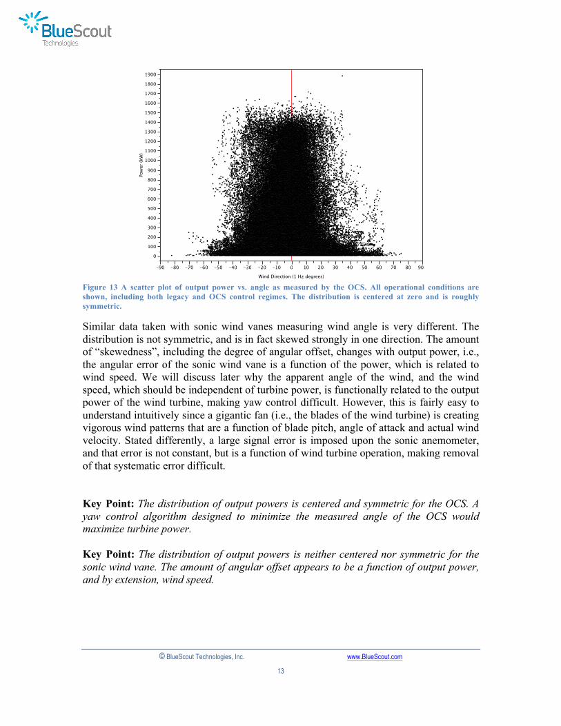
Measurement Asymmetry To further investigate the disparity between the angles measured by the sonic wind vane and the OCS, we simply generated a scatter plot of power generated vs. measured angle. In this comparison, we are showing all data, whether the system was controlled by the legacy system or the OCS. If we plot power vs. OCS angle, we see a distribution with a rather flat top, being limited by the rated power of the turbine, roughly centered at angle = 0, with the distributions being rather symmetric around zero. This distribution is what would be intuitively expected.


13

Figure 13 A scatter plot of output power vs. angle as measured by the OCS. All operational conditions are shown, including both legacy and OCS control regimes. The distribution is centered at zero and is roughly symmetric.

Similar data taken with sonic wind vanes measuring wind angle is very different. The distribution is not symmetric, and is in fact skewed strongly in one direction. The amount of “skewedness”, including the degree of angular offset, changes with output power, i.e., the angular error of the sonic wind vane is a function of the power, which is related to wind speed. We will discuss later why the apparent angle of the wind, and the wind speed, which should be independent of turbine power, is functionally related to the output power of the wind turbine, making yaw control difficult. However, this is fairly easy to understand intuitively since a gigantic fan (i.e., the blades of the wind turbine) is creating vigorous wind patterns that are a function of blade pitch, angle of attack and actual wind velocity. Stated differently, a large signal error is imposed upon the sonic anemometer, and that error is not constant, but is a function of wind turbine operation, making removal of that systematic error difficult.

Key Point: The distribution of output powers is centered and symmetric for the OCS. A yaw control algorithm designed to minimize the measured angle of the OCS would maximize turbine power. Key Point: The distribution of output powers is neither centered nor symmetric for the sonic wind vane. The amount of angular offset appears to be a function of output power, and by extension, wind speed.

Journal: untitled journal 3 Page 1 of 3

0

100

200

300

400

500

600

700

800

900

1000

1100

1200

1300

1400

1500

1600

1700

1800

1900

Pow

er (k

W)

-90 -80 -70 -60 -50 -40 -30 -20 -10 0 10 20 30 40 50 60 70 80 90

Wind Direction (1 Hz degrees)

Power vs. OCS Wind Direction

Power vs 60 sec MA of A1


14

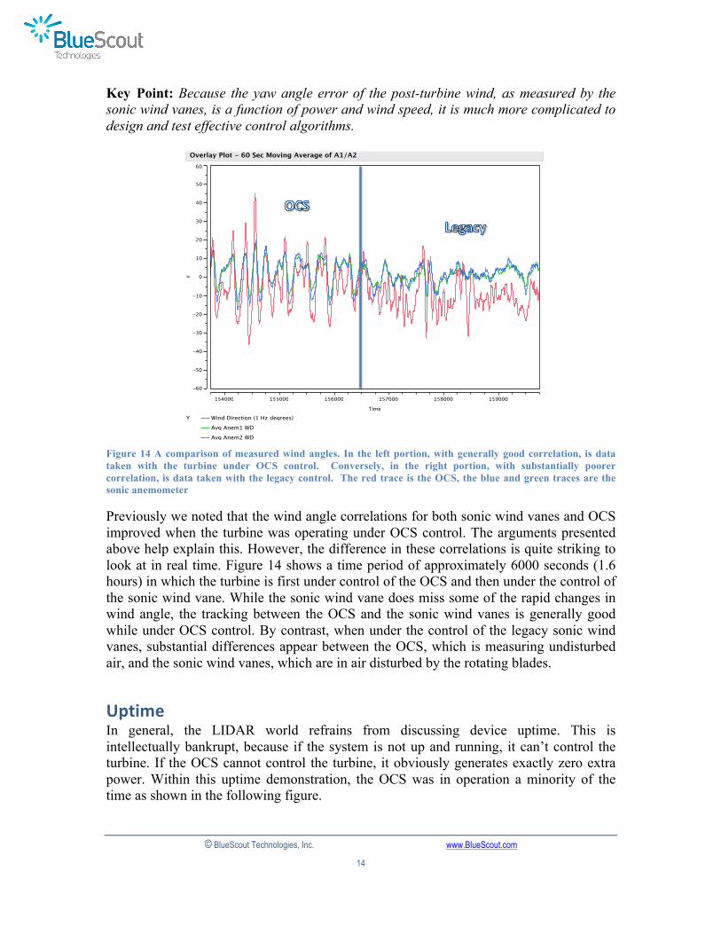
Key Point: Because the yaw angle error of the post-turbine wind, as measured by the sonic wind vanes, is a function of power and wind speed, it is much more complicated to design and test effective control algorithms.

Figure 14 A comparison of measured wind angles. In the left portion, with generally good correlation, is data taken with the turbine under OCS control. Conversely, in the right portion, with substantially poorer correlation, is data taken with the legacy control. The red trace is the OCS, the blue and green traces are the sonic anemometer

Previously we noted that the wind angle correlations for both sonic wind vanes and OCS improved when the turbine was operating under OCS control. The arguments presented above help explain this. However, the difference in these correlations is quite striking to look at in real time. Figure 14 shows a time period of approximately 6000 seconds (1.6 hours) in which the turbine is first under control of the OCS and then under the control of the sonic wind vane. While the sonic wind vane does miss some of the rapid changes in wind angle, the tracking between the OCS and the sonic wind vanes is generally good while under OCS control. By contrast, when under the control of the legacy sonic wind vanes, substantial differences appear between the OCS, which is measuring undisturbed air, and the sonic wind vanes, which are in air disturbed by the rotating blades.

Uptime In general, the LIDAR world refrains from discussing device uptime. This is intellectually bankrupt, because if the system is not up and running, it can’t control the turbine. If the OCS cannot control the turbine, it obviously generates exactly zero extra power. Within this uptime demonstration, the OCS was in operation a minority of the time as shown in the following figure.


-60

-50

-40

-30

-20

-10

0

10

20

30

40

50

60

Y

154000 155000 156000 157000 158000 159000

Time

Overlay Plot - 60 Sec Moving Average of A1/A2

Y Wind Direction (1 Hz degrees)

Avg Anem1 WD

Avg Anem2 WD


15

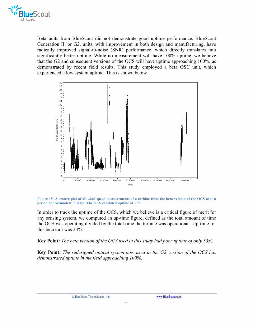
Beta units from BlueScout did not demonstrate good uptime performance. BlueScout Generation II, or G2, units, with improvement in both design and manufacturing, have radically improved signal-to-noise (SNR) performance, which directly translates into significantly better uptime. While no measurement will have 100% uptime, we believe that the G2 and subsequent versions of the OCS will have uptime approaching 100%, as demonstrated by recent field results. This study employed a beta OSC unit, which experienced a low system uptime. This is shown below.

Figure 15 A scatter plot of all wind speed measurements of a turbine from the beta version of the OCS over a period approximately 30 days. The OCS exhibited uptime of 33%.

In order to track the uptime of the OCS, which we believe is a critical figure of merit for any sensing system, we computed an up-time figure, defined as the total amount of time the OCS was operating divided by the total time the turbine was operational. Up-time for this beta unit was 33%. Key Point: The beta version of the OCS used in this study had poor uptime of only 33%. Key Point: The redesigned optical system now used in the G2 version of the OCS has demonstrated uptime in the field approaching 100%.


1

2

3

4

5

6

7

8

9

10

11

12

13

14

15

16

17

18

19

20

21

22

23

24

2526

Win

d Sp

eed

(1H

z m

/s)

0 250000 500000 750000 1000000 1250000 1500000 1750000 2000000 2250000

Time

Overlay Plot


16

Turbine Power Production

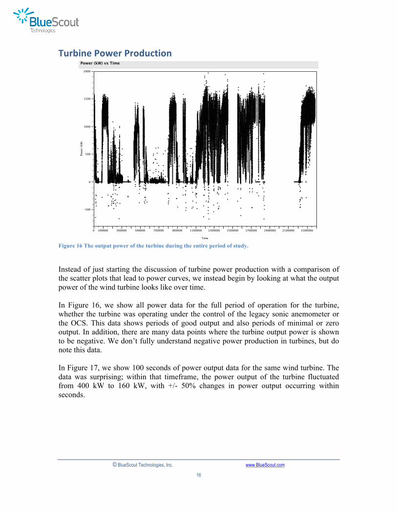
Figure 16 The output power of the turbine during the entire period of study.

Instead of just starting the discussion of turbine power production with a comparison of the scatter plots that lead to power curves, we instead begin by looking at what the output power of the wind turbine looks like over time. In Figure 16, we show all power data for the full period of operation for the turbine, whether the turbine was operating under the control of the legacy sonic anemometer or the OCS. This data shows periods of good output and also periods of minimal or zero output. In addition, there are many data points where the turbine output power is shown to be negative. We don’t fully understand negative power production in turbines, but do note this data. In Figure 17, we show 100 seconds of power output data for the same wind turbine. The data was surprising; within that timeframe, the power output of the turbine fluctuated from 400 kW to 160 kW, with +/- 50% changes in power output occurring within seconds.

Nordex Data: Overlay Plot of Power (kW) by Time Page 1 of 1

-500

0

500

1000

1500

2000

Pow

er (

kW)

0 100000 300000 500000 700000 900000 1100000 1300000 1500000 1700000 1900000 2100000 2300000

Time

Power (kW) vs Time


17

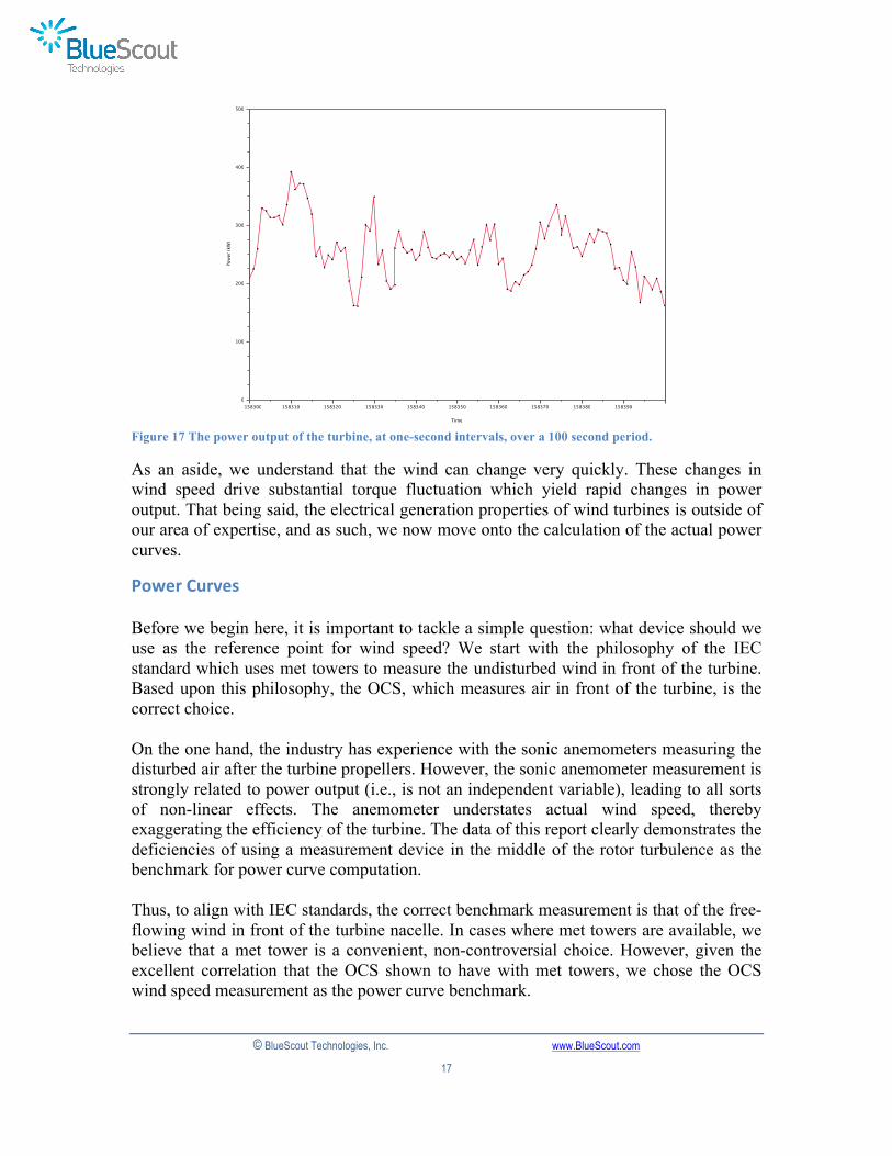
Figure 17 The power output of the turbine, at one-second intervals, over a 100 second period.

As an aside, we understand that the wind can change very quickly. These changes in wind speed drive substantial torque fluctuation which yield rapid changes in power output. That being said, the electrical generation properties of wind turbines is outside of our area of expertise, and as such, we now move onto the calculation of the actual power curves.

Power Curves Before we begin here, it is important to tackle a simple question: what device should we use as the reference point for wind speed? We start with the philosophy of the IEC standard which uses met towers to measure the undisturbed wind in front of the turbine. Based upon this philosophy, the OCS, which measures air in front of the turbine, is the correct choice. On the one hand, the industry has experience with the sonic anemometers measuring the disturbed air after the turbine propellers. However, the sonic anemometer measurement is strongly related to power output (i.e., is not an independent variable), leading to all sorts of non-linear effects. The anemometer understates actual wind speed, thereby exaggerating the efficiency of the turbine. The data of this report clearly demonstrates the deficiencies of using a measurement device in the middle of the rotor turbulence as the benchmark for power curve computation. Thus, to align with IEC standards, the correct benchmark measurement is that of the free-flowing wind in front of the turbine nacelle. In cases where met towers are available, we believe that a met tower is a convenient, non-controversial choice. However, given the excellent correlation that the OCS shown to have with met towers, we chose the OCS wind speed measurement as the power curve benchmark.

Nordex_Turbine_OCS_online_turbine_time: Overlay Plot of Power (kW) by Time Page 1 of 1

0

100

200

300

400

500

Pow

er (

kW)

158300 158310 158320 158330 158340 158350 158360 158370 158380 158390

Time

Overlay Plot


18

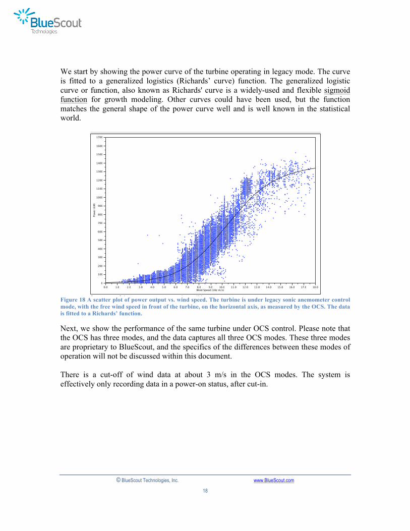
We start by showing the power curve of the turbine operating in legacy mode. The curve is fitted to a generalized logistics (Richards’ curve) function. The generalized logistic curve or function, also known as Richards' curve is a widely-used and flexible sigmoid function for growth modeling. Other curves could have been used, but the function matches the general shape of the power curve well and is well known in the statistical world.

Figure 18 A scatter plot of power output vs. wind speed. The turbine is under legacy sonic anemometer control mode, with the free wind speed in front of the turbine, on the horizontal axis, as measured by the OCS. The data is fitted to a Richards’ function.

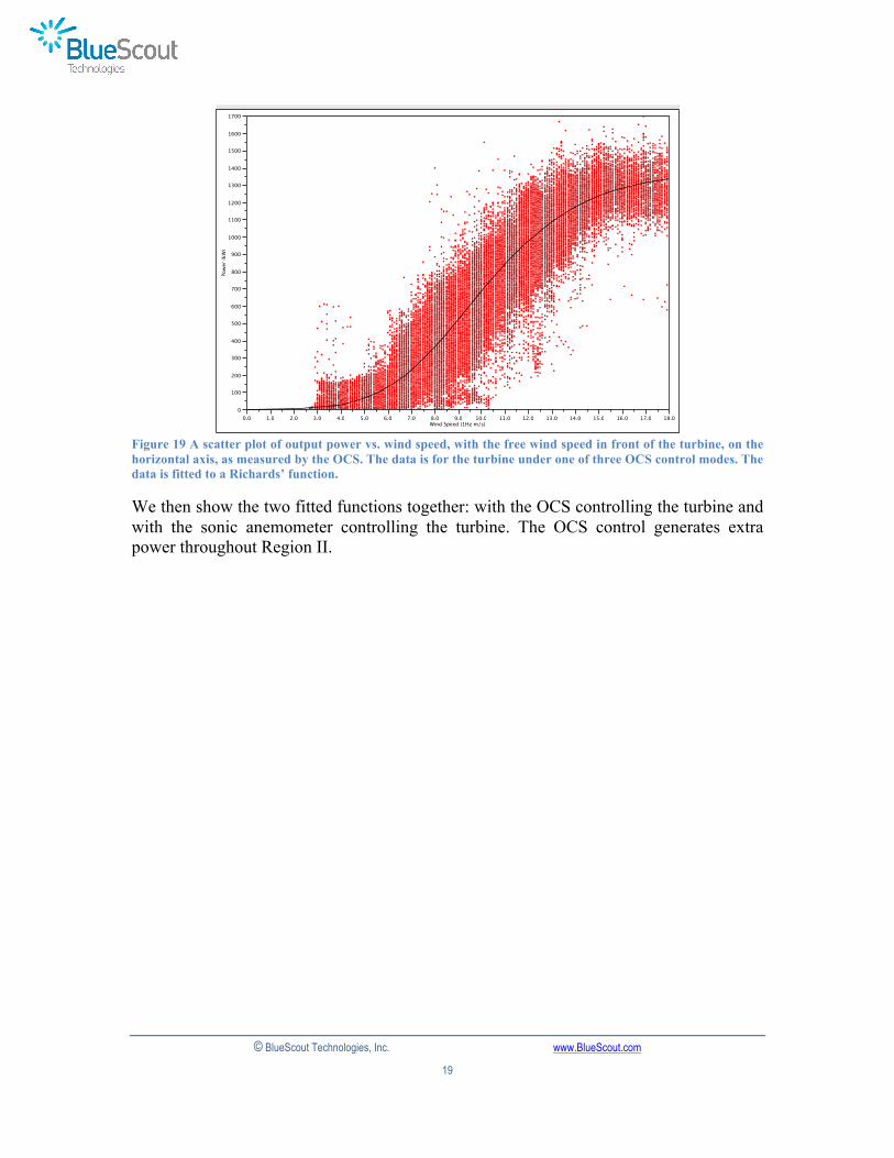
Next, we show the performance of the same turbine under OCS control. Please note that the OCS has three modes, and the data captures all three OCS modes. These three modes are proprietary to BlueScout, and the specifics of the differences between these modes of operation will not be discussed within this document. There is a cut-off of wind data at about 3 m/s in the OCS modes. The system is effectively only recording data in a power-on status, after cut-in.

Nordex_Turbine_OSC_online: Nonlinear Page 1 of 2

Response: Power (kW), Predictor: Column 35

0

100

200

300

400

500

600

700

800

900

1000

1100

1200

1300

1400

1500

1600

1700

Pow

er (k

W)

0.0 1.0 2.0 3.0 4.0 5.0 6.0 7.0 8.0 9.0 10.0 11.0 12.0 13.0 14.0 15.0 16.0 17.0 18.0Wind Speed (1Hz m/s)

theta1theta2theta3theta4theta5

Parameter0

1382.79215694.2339636201-0.4431492561.3803824449

Estimate5e-101

653.3931.98155-0.69980.81616

Low2e-100

1960.185.94464-0.23332.44847

High

Plot

Nonlinear Fit OCS Controlling=0



19

Figure 19 A scatter plot of output power vs. wind speed, with the free wind speed in front of the turbine, on the horizontal axis, as measured by the OCS. The data is for the turbine under one of three OCS control modes. The data is fitted to a Richards’ function.

We then show the two fitted functions together: with the OCS controlling the turbine and with the sonic anemometer controlling the turbine. The OCS control generates extra power throughout Region II.

Nordex_Turbine_OSC_online: Nonlinear Page 2 of 2Nonlinear Fit OCS Controlling=0

Response: Power (kW), Predictor: Column 35

0

100

200

300

400

500

600

700

800

900

1000

1100

1200

1300

1400

1500

1600

1700

Pow

er (k

W)

0.0 1.0 2.0 3.0 4.0 5.0 6.0 7.0 8.0 9.0 10.0 11.0 12.0 13.0 14.0 15.0 16.0 17.0 18.0Wind Speed (1Hz m/s)

theta1theta2theta3theta4theta5

Parameter0

1390.02750752.4530321336-0.3779418213.0026449335

Estimate5e-101

653.3931.98155-0.69980.81616

Low2e-100

1960.185.94464-0.23332.44847

High

Plot



20

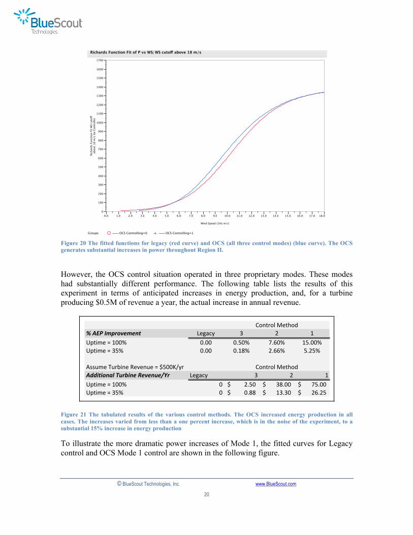
Figure 20 The fitted functions for legacy (red curve) and OCS (all three control modes) (blue curve). The OCS generates substantial increases in power throughout Region II.

However, the OCS control situation operated in three proprietary modes. These modes had substantially different performance. The following table lists the results of this experiment in terms of anticipated increases in energy production, and, for a turbine producing $0.5M of revenue a year, the actual increase in annual revenue.

Figure 21 The tabulated results of the various control methods. The OCS increased energy production in all cases. The increases varied from less than a one percent increase, which is in the noise of the experiment, to a substantial 15% increase in energy production

To illustrate the more dramatic power increases of Mode 1, the fitted curves for Legacy control and OCS Mode 1 control are shown in the following figure.

Nordex_Turbine_OSC_online: Overlay Plot of Richards Function Fit WS cutoff above 18 m/s by Controller by Wind Speed (1Hz m/s) Page 1 of 1

0

100

200

300

400

500

600

700

800

900

1000

1100

1200

1300

1400

1500

1600

1700

Rich

ards

Fun

ctio

n Fi

t WS

cutoff

abov

e 18

m/s

by

Cont

rolle

r

0.0 1.0 2.0 3.0 4.0 5.0 6.0 7.0 8.0 9.0 10.0 11.0 12.0 13.0 14.0 15.0 16.0 17.0 18.0

Wind Speed (1Hz m/s)

Richards Function Fit of P vs WS; WS cutoff above 18 m/s

Groups OCS Controlling=0 OCS Controlling=1

%"AEP"Improvement Legacy 3 2 1Uptime/=/100% 0.00 0.50% 7.60% 15.00%Uptime/=/35% 0.00 0.18% 2.66% 5.25%

Assume/Turbine/Revenue/=/$500K/yrAdditional"Turbine"Revenue/Yr Legacy 3 2 1Uptime/=/100% 0 2.50$////////// 38.00$//////// 75.00$//////// /Uptime/=/35% 0 0.88$////////// 13.30$//////// 26.25$////////

Control/Method

Control/Method


21

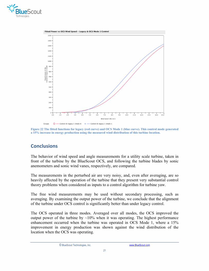
Figure 22 The fitted functions for legacy (red curve) and OCS Mode 1 (blue curve). This control mode generated a 15% increase in energy production using the measured wind distribution of this turbine location.

Conclusions The behavior of wind speed and angle measurements for a utility scale turbine, taken in front of the turbine by the BlueScout OCS, and following the turbine blades by sonic anemometers and sonic wind vanes, respectively, are compared. The measurements in the perturbed air are very noisy, and, even after averaging, are so heavily affected by the operation of the turbine that they present very substantial control theory problems when considered as inputs to a control algorithm for turbine yaw. The free wind measurements may be used without secondary processing, such as averaging. By examining the output power of the turbine, we conclude that the alignment of the turbine under OCS control is significantly better than under legacy control. The OCS operated in three modes. Averaged over all modes, the OCS improved the output power of the turbine by ~10% when it was operating. The highest performance enhancement occurred when the turbine was operated in OCS Mode 1, where a 15% improvement in energy production was shown against the wind distribution of the location when the OCS was operating.


22

The beta version OCS had substantial periods of time when it was not collecting good data, and by extension, was not controlling the turbine. This is being improved in the G2 version of the OCS. For the period of time studied here, the uptime of the beta OCS was 33%. In future G2 units, we anticipate that the uptime of the device will be close to 100%.

Documents

BlueScout 1 Wind Measurements and Power