Embed Size (px)
Citation preview

1
BLUE: Behaviour Lifestyles and Uncertainty Energy model
Online Documentation Revision 04, Version 2.3, January 2019
Francis G. N. Lia, [email protected]
Neil Strachana, [email protected]
aUCL Energy Institute, Central House, 14 Upper Woburn Place, London, WC1H 0NN, United Kingdom
1.0 Overview
This document gives a description of the key features, mathematical equations and data used for the Behaviour, Lifestyles and Uncertainty Energy model (BLUE). The documentation will be periodically updated in line with major modifications and extensions to the model. In the interest of transparency and being able to identify which revisions of the model have been used to produce different publications [1], a list of publications and associated model version numbers is maintained under Section 7.0 of the documentation.
BLUE is a system dynamic model of the UK energy system that simulates technological change, energy use, and emissions. A defining feature of the model is the ability to simulate the individual behaviours of multiple energy system actors who interact dynamically through time as changes to technologies, demands, and prices unfold.
BLUE aims to enhance the policy relevance of energy system modelling by explicitly addressing deviations from strict economic rationality found in the behavioural economics literature and also by enabling technological diffusion to be directly related to decisions made by multiple representative agents. The model employs a stochastic Monte Carlo formulation which makes it particularly well-suited for exploring energy transitions under conditions of deep uncertainty. BLUE has been designed to complete a full set of simulations in a matter of minutes. This rapid run time, alongside multi-agent simulation, potentially makes the model suitable for participatory modelling with stakeholders [2] as a means of promoting learning and critical thinking about energy system futures, and consensus building amongst disparate actors [3].
2.0 Implementation and System Requirements
The equations and data for the BLUE model are implemented in Analytica, a visual software environment for quantitative decision models. For more details see the developers’ website: http://www.lumina.com/why-analytica/what-is-analytica1/. The roots of Analytica can be found in the decision tools developed by Granger and Henrion in their seminal publication on decision making under uncertainty [4].

2
Analytica currently is provided as a native Microsoft Windows binary and requires a virtualisation environment to run on Apple Mac OS or Linux systems. The principal performance bottleneck found in large Analytica models is system memory. It is recommended that the BLUE model is run on systems with at least 4GB RAM.
3.0 Brief Description
BLUE is a system dynamic simulation model that shares key concepts with so-called bottom-up hybrids [5] such as the Canadian Integrated Modelling System (CIMS) [6], PRIMES [7], POTeNCIA [8], or the IMpact Assessment of CLIMate policies (IMACLIM) model family [9]. BLUE simulates decisions taken in different economic sectors using multiple representative agents. The dynamics of the system are dominated by a number of agents that are relatively few in number (i.e. tens, not thousands) and so BLUE is closer to what is termed in the literature as an “actor-based” model [10] rather than what many researchers might call an “agent-based model” (at least in the classic sense implied by Epstein and Axtell [11]). BLUE occupies an interesting space in the landscape of energy system simulation models. BLUE is more disaggregated in its representation of decision makers in the energy system than models that take a social planning perspective (which often only have a single representative agent), but it does not feature extremely granular micro-simulation with a population of thousands of individual agents. The model also aims to capture energy system interactions across multiple sectors (industrial, residential, transport etc.) rather than focusing on individual sectors. The system-wide perspective is critical for understanding economy-wide decarbonisation targets in the context of climate policy assessment. The model is designed for addressing “exploratory” scenario analysis activities (in the sense implied by Börjeson [12]) rather than backcasting from normative targets [13].
In BLUE, representative agents make decisions independently of one another, with some sectors captured with a single agent whereas others use multiple agents (discussed further in Section 4.0). Sector-based actors are responsible for capital stock replacement in their own domains. As capital assets reach the end of their economic lives and are retired, each sector-specific decision maker has a window of opportunity to replace assets on either a like-for-like basis or to switch investment into new technologies. The government is captured as a separate type of actor that does not directly make decisions on capital assets but rather influences the macro-scale techno-economic conditions for investment across the whole system.
The non-government actors in BLUE carry out value appraisals from their own perspectives, attempting to minimise their overall individual costs with imperfect knowledge of how other actors in the energy system might respond to their actions. Each actor makes myopic choices and they do not possess advance knowledge of what future changes to landscape conditions such as fuel prices, social preferences, and technology performance/costs might be. The myopia in the model takes the form of decisions by different actors being taken across a series of discrete time horizons that correspond to expected technology lifetimes. These do not overlap, and so the myopic formulation can be characterised as being of the “limited foresight” type

3
(rather than the “moving decision window” type) in the classic taxonomy of myopic energy system models by Keppo and Strubegger [14].
BLUE therefore captures system level energy demand, emissions, and technological diffusion as emergent phenomena resulting from the interaction of the different representative agents across the time horizon. BLUE employs Monte Carlo simulation (with n=500 by default) to capture parametric uncertainty, which can result from any of the inputs, be they technological, economic, or behavioural.
Figure 1- Model Topology
4.0 Actors and Behaviour
4.1 Overview of Actor Types
BLUE features a range of representative agents that are used to depict various transition actors within the energy system. Some sectors are depicted with a single decision-maker, while others use multiple representative agents that have differentiated behavioural settings (details are given later in Section 7.0). These are adapted from Rogers classic taxonomy of the diffusion of innovations [15] and are termed: innovators, early adopters, early majority, late majority, and laggards.
Each representative agent has different levels of agency when it comes to their influence over the energy system. Notably, the representative agent for the Government actor is the only one that can affect macro-scale conditions for investment across the entire system.

4
Table 1 – System Actors, Representative Agents and Agency
System Actor Representative Agents Agency
Government Single representative agent for the
Government
Decisions over economy wide CO2 pricing
Decisions over subsidies for technologies in all sectors
Decisions over technology regulation in all sectors
Power Generation
Single representative agent for the Power sector
Decisions over electricity generation investment
Commercial Buildings
Single representative agent for all Commercial buildings
Decisions over heating system replacement in commercial buildings
Residential Buildings
Five representative agents, each depicting a stylised social group: innovators, early
adopters, early majority, late majority, and laggards
Decisions over heating system replacement
Decisions on investment in microgeneration
Decisions on investment in highly thermally efficient buildings
Industrial Single representative agent for all Industrial
energy use Decisions over fuel switching to meet
industrial process demand
Road Transport
Five representative agents, each depicting a stylised social group: innovators, early
adopters, early majority, late majority, and laggards
Decisions over road transport choices
Air Transport Single representative agent for Air transport No technological or fuel switching options in
current model version
Rail Transport Single representative agent for Rail transport No technological or fuel switching options in
current model version
Marine Transport
Single representative agent for Marine transport
No technological or fuel switching options in current model version
4.2 Government Actor Behaviour
The Government actor in BLUE monitors progress towards economy-wide decarbonisation targets and attempts to change the macro-scale environment for investment in technologies for the other actors. Key equations are provided in Section 5.0. The Government actor is able to act via two principal means:
An economy-wide CO2 tax on emissions which affects all fuels in all sectors.
Regulating against polluting fossil fuel technologies
The ability of the government to increase the CO2 tax is imagined as being societally constrained. BLUE employs the idea of a societal mandate [16] for the transition, based on the proportion of the electorate who own low carbon technologies. Conceptually, it is assumed that ownership of low carbon technologies effectively

5
creates a constituency of voters (following Patashnik [17] and Lockwood [18]) in favour of decarbonisation.
Regulation takes the form of subsidies for low-carbon technologies and bans for polluting technologies. These are currently operationalised in the model as taking effect when low-carbon technologies comprise different fractions of market share, allowing the model to represent both conditions where the government is supporting/penalising a mainstream technology or supporting/penalising a niche one. The thresholds are currently implemented as user-defined exogenous parameters, that can be set during exploratory scenario exercises.
4.3 Non-State Actor Behaviour
Representative agents (with the exception of the Government actor, who is treated differently as discussed in Section 4.2) can be configured with a range of behavioural parameters, including:
Demand elasticities e, describing actor sensitivity to changes in prices
Market heterogeneity v, describing actor propensity to cost-optimise
Intangible costs i, describing actor perception of non-monetary costs
Hurdle rates r, describing actor sensitivity to up-front investment
Retrofitting/replacement rate b, describing actor investment cycles
The behavioural parameters in BLUE can strongly influence system behaviour, and end users are encouraged to implement and test their own data ranges. The default settings assume that the behaviour of firms is more cost driven then that of individuals.
4.3.1 Demand Elasticities, e
Demand elasticities for each representative agent are described in Section 6.0. These are mostly drawn from a review of the literature for each modelled sector conducted by Pye et al. [19].
4.3.2 Market Heterogeneity, v
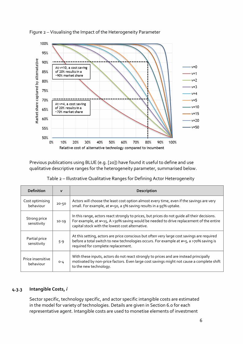
Section 6.0 contains details of the default settings for each representative agent. The effects of adopting different values for the heterogeneity parameter, v are illustrated below with an example comparing two technologies against one another. As v approaches zero, the costs of different options play little to no role in investment choices (i.e. implying that non-monetary factors are the driver), while for high values of v the model displays highly cost optimising behaviour (i.e. even a tiny percentage saving in costs is enough to trigger a switch from one option to the other).
6
Figure 2 – Visualising the Impact of the Heterogeneity Parameter
Previous publications using BLUE (e.g. [20]) have found it useful to define and use qualitative descriptive ranges for the heterogeneity parameter, summarised below.
Table 2 – Illustrative Qualitative Ranges for Defining Actor Heterogeneity
Definition v Description
Cost optimising behaviour
20-50 Actors will choose the least cost option almost every time, even if the savings are very small. For example, at v=50, a 5% saving results in a 95% uptake.
Strong price sensitivity
10-19 In this range, actors react strongly to prices, but prices do not guide all their decisions. For example, at v=15, A >30% saving would be needed to drive replacement of the entire capital stock with the lowest cost alternative.
Partial price sensitivity
5-9 At this setting, actors are price conscious but often very large cost savings are required before a total switch to new technologies occurs. For example at v=5, a >70% saving is required for complete replacement.
Price insensitive behaviour
0-4 With these inputs, actors do not react strongly to prices and are instead principally motivated by non-price factors. Even large cost savings might not cause a complete shift to the new technology.
4.3.3 Intangible Costs, i
Sector specific, technology specific, and actor specific intangible costs are estimated in the model for variety of technologies. Details are given in Section 6.0 for each representative agent. Intangible costs are used to monetise elements of investment

7
decision-making that are not explained by direct financial costs (e.g. transaction costs and other negative externalities [21]). Negative intangible costs might be interpreted as non-financial co-benefits.
4.3.4 Hurdle Rates, r
Representative agents use a variety of hurdle rates in their decision making, which is an indicator of their sensitivity to up-front investment costs. The default calibration for each representative agent is described in Section 6.0. The financial cost of capital available to individuals and private companies might range from 9-17% [22], whereas it is more common for policy assessment activities to be conducted with a longer term perspective on valuing the future (due to considerations such as intergenerational equity [23]) using rates of 3-6% [24,25].
The UK government recommends a social discount rate of 3.5% [24] and outputs from most energy economic models represent economically rational choices made from the perspective of maximising social utility. Energy system optimisation models (ESOMs) like MESSAGE [26], TIMES/MARKAL [27], OSEMoSYS [28] etc. are therefore often set up by analysts to assume social discount rates (typically ~3%).
However, there are a wide range of factors that cause individual choices to deviate from the social optimum. Individual actors are exposed to investment risks in the way which society at large is not because their assets are not as diversified [29]. While individuals might analyse investments based on say, a market rate of 15%, revealed discount rates i.e. what rates are implicit in actual decision-making, can actually be much higher, and have even been estimated as being high as 30%, 50%, or even 80% [30].
5.0 Key Equations
5.1 Energy Service Demands and Energy Prices
Energy service demands are assumed to grow in line with user-defined exogenous drivers that are calibrated to reflect individual national circumstances. Energy service demands are affected by demand elasticity parameters and the rate of change in energy prices between t=t and t=1-1. This is expressed as:
𝐷𝑠,𝑡 = 𝐷𝑠,𝑡−1 × [1 + 𝐺𝑠] × [𝑒𝑠,𝑡−1(1 − ∆𝑃𝑠,𝑡−1)] (1)
Where D = energy service demand, s = sector, t = time period, G = demand driver, P = energy price, and e = price elasticity of demand.
Energy prices grow by a user input rate through time, which can be aligned with policy projections or randomised as desired by the user. Energy prices contain a fuel price component and a carbon price component.

8
𝐸𝑓,𝑡 = [𝑃𝑓,𝑡−1 × (1 + 𝑘𝑓)] + [𝑧𝑓,𝑡 × {𝐶𝑂2,𝑡−1 × (1 + 𝑗)}] (2)
Where E = energy price, P = fuel price, t = time period, f = fuel type, k = periodic fuel price increase/decrease, CO2 = carbon price, j = periodic carbon price increase/decrease and z = specific emissions intensity.
5.2 Capital Stock Replacement
Each sector evaluates the net present value of competing technology options. The net present value of available technologies is expressed as:
𝑁𝑠,𝑡,𝑥 = 𝐶𝑠,𝑡,𝑥 + 𝑖𝑠,𝑡,𝑥 + 𝑞𝑠,𝑡,𝑥 − 𝑢𝑠,𝑡,𝑥 + ∑ [𝐷𝑠,𝑡×𝑃𝑓,𝑡×𝑌𝑠,𝑡,𝑥
−1
(1+𝑟𝑠,𝑡)𝑡 ]𝑇
𝑡 (3)
Where N = net present value, s = sector, t = time period, x = energy technology, C = investment cost, i = intangible cost, q = pigouvian tax from government, u = government subsidy, D = energy service demand, f = fuel type, Y = efficiency, r = hurdle rate, T =investment time horizon
The net present value then serves as an input into the model’s evaluation of technology diffusion into the marketplace.
𝑀𝑠,𝑡,𝑥 = [𝑀𝑠,𝑡−1,𝑥 × (1 − 𝑏𝑠,𝑡)] + [𝑀𝑠,𝑡−1 × 𝑏𝑠,𝑡 × (𝑁𝑠,𝑡
−𝑣𝑠,𝑡
∑ 𝑁𝑠,𝑡
−𝑣𝑠,𝑡𝑥
)] (4)
Where M = technology portfolio, s = sector, t = time period, x = energy technology, b = retrofitting/replacement rate, N = net present value, v = heterogeneity parameter
5.3 Government Decision-Making and Government-Society Relations
The government tracks the total level of CO2 emissions across the economy in each annual time slice against the CO2 emission trajectory implied by a linear decarbonisation pathway between the 1990 base year specified in UK law and the target date:
∆𝑡𝑎𝑟𝑔𝑒𝑡= 𝐸𝑚𝑡 ((𝑡 − 1) × [𝐸𝑚𝑡𝑎𝑟𝑔𝑒𝑡−𝐸𝑚1990
𝑌]) (5)
Where target = distance to target trajectory, Emt = emissions in current time period, Emtarget = emissions target, Em1990 = emissions in 1990, Y = time horizon for the energy transition, t = time period
If the model is on target or ahead of target (target = 0 or target = negative) and reducing emissions in line with the assessment trajectory, no further action is taken. If
the model if off target (target = positive), however, then the government is considered to have failed to reduce emissions for that year. A failure counter (described below) tracks the total number of cumulative failure years.

9
Following a failure year, the Government actor tries to change the macro-scale investment conditions across the energy system by raising the CO2 tax by a percentage indexed to the societal mandate for the energy transition (equation 7). Conceptually the normative ideal is for a fossil-fuel free system, so we imagine that a society with complete buy-in (again, following the idea that ownership implies a constituency in favour of the transition, discussed in Section 4.2) to the idea of such an energy transition (100% mandate) would imply a society where all power and transport was without fossil fuels, and all heating was as low-carbon as possible.
The rate of change for the CO2 tax year on year is scaled (divided by 10) to be between 0 – 10% in this model version. The basis for this is that an increase of 10% per annum implies a doubling every 7 years, which by any measure of systemic change is a very rapid rate of increase. The carbon tax in any given year can therefore be given as:
𝐶𝑂2𝑡𝑎𝑥,𝑡 = 𝐶𝑂2𝑡𝑎𝑥,𝑡−1 × (1 +𝑆𝑀
10) (6)
Where CO2tax = the carbon price, t = time period, SM = societal mandate (see below)
Additionally, if the total number of cumulative failure years increases above user defined threshold (currently this is set to 3 years) then there is an arbitrary collapse in the carbon price for a single year (currently set to 10%).
The societal mandate is currently computed as the average market share across the power, heating and transport sectors:
𝑆𝑀 =[𝑀𝑆𝑝+𝑀𝑆ℎ+𝑀𝑆𝑡]
3 (7)
Where SM = societal mandate, MSp = market share of non-fossil fuel power, MSh = market share of non-fossil fuel heating, MSt = market share of non-fossil fuel transport
The Government actor can also be set up by the model operator to intervene in specific sectors. The model tracks the market share of all technologies, with fossil fuel technologies tracked separately from non-fossil fuel options. Both Pigouvian taxes on polluting fossil fuel technologies and subsidies for non-fossil fuel technologies can be levied up to certain user-defined thresholds of market share in individual sectors. These are included in the description of capital cost computation above under Section 5.2.
The rate of change for the proportion of the population in each societal group (from the base year defined in Section 6.2) is also influenced by the societal mandate. The change driver is scaled so that the largest year-on-year change between groups is 10% (again, this is a very rapid rate of change that is used as a plausible upper limit in the current model version). The population moves between adjacent groups, so that all intermediate groups have a source group and a destination group. Laggards move to become late majority, late majority become early majority, early majority become early adopters, and early adopters become innovators. For intermediate groups we can write this as:

10
𝑃𝑔,𝑡 = 𝑃𝑔,𝑡−1 + [𝑃𝑗,𝑡−1 × (1 +𝑆𝑀
10)] − [𝑃𝑔,𝑡−1 × (1 +
𝑆𝑀
10)] (8)
Where P = population fraction, g = current societal group, j = source societal group, t = time period, SM = societal mandate
6.0 Data Sources and Calibration
6.1 Base Year Energy Service Demands
The BLUE model is calibrated for the United Kingdom using official government statistics and a 2010 base year. Energy service demands originally given in other units are converted to petajoules (PJ).
Table 3 – BLUE Base Year Energy Service Demands
Parameter Sub-Parameter Value
(L=Low, C=Central, H=High) Units Notes
Energy Service Demands
Residential
Commercial
Industrial
Transport (Road)
Transport (Air)
Transport (Rail)
Transport (Marine)
2064
821
1093
1691
515
42
38
PJ UK Department of Energy and Climate Change (DECC) [31].
6.2 Population and Societal Groups
The population in the base year is calibrated to UK National Statistics. The growth rate is set to a linear annual increase of 0.51% in order to align with government population projections. In the absence of other assumptions, this trend continues out to the end of the model time horizon in 2070. The base year societal groupings for the innovator, early adopters, early majority, late majority, and laggard categories are taken from Rogers [15].
Table 4 – BLUE Population and Societal Groups
Parameter Sub-Parameter Value Units Notes
Population Population 2010
Growth Rate
62.76
0.51
million
%
UK Office of National Statistics, Table A1-1, Principal Projection - UK Summary, 2012-based [32]

11
Societal Groups
Innovators
Early Adopters
Early Majority
Late Majority
Laggards
2.5
13.5
34
34
16
% Rogers [15]
6.3 Fuel Costs and Emission Factors
BLUE currently employs a stylised representation of fuel types. For example, various types of liquid transport fuels are aggregated together into “Oil”, while different coal grades (e.g. bituminous coal, anthracite, etc.) are covered by “Coal”. Electricity costs and emission intensities are determined dynamically based on the generation portfolio used in each time period (see below).
Table 5 – BLUE Fuel Costs and Emission Factors
Parameter Sub-Parameter
Value
(L=Low, C=Central, H=High)
Units Notes
Fossil Fuel Prices
Oil
Coal
Gas
Dynamic
Dynamic
Dynamic
£/GJ
Users can select low / medium / high projections or capture all trajectories as a triangular distribution.
Costs are based on projections from UK Department of Energy and Climate Change (DECC) [33].
Fossil Fuel Emission Intensities
Oil
Coal
Gas
0.0917
0.0763
0.0517
tCO2/GJ US Energy Information Administration (EIA) [34]
6.4 Power Generation
6.4.1 Behavioural Calibration
The power sector uses a single representative agent that acts to balance energy demand with (time delayed) investments in generation technologies. The default model assumptions are that this actor makes decisions that are highly cost driven.
Table 6 – Behavioural Parameters for Power Sector (L=Low, C=Central, H=High)
Behavioural Parameter Commercial
Demand elasticities (e), see Section 4.3.1 -
Market heterogeneity (v), see Section 4.3.2 Cost optimising behaviour, L=20, H=50
Intangible costs (i), see Section 4.3.4 -
Hurdle rate (r), see Section 4.3.4 Implicit in LCOE (see Table 7)

12
Retrofit / replacement rate (b), see Section 4.3.5 Technology specific, based on [35,36]
6.4.2 Technologies
BLUE employs 9 different power technologies that characterise the base year generation fleet as well as capturing future options for electricity supply. The techno-economic performance of different options is expressed in terms of their levelised costs of energy (LCOE, see [37]), which is determined from unit estimates of capital costs, fixed operation and maintenance costs, and variable operation and maintenance costs taken from a range of government and academic sources (see below). BLUE’s stylized representation of the power sector determines total generation requirements against a user defined capacity margin, while the contribution to total capacity requirements from individual technologies varies by technology.
Table 7 –Technology Parameters for Power Generation Sector
Parameter Sub-Parameter Value
(L=Low, C=Central, H=High) Units Notes
Power Generation Technology Portfolio
Gas
Coal
Coal-CCS
Gas-CCS
Nuclear
Onshore Wind
Offshore Wind
Large Scale Solar PV
Bioenergy-CCS
35.3
35.8
0
0
10.9
0
4.218
0
0
GW UK Department of Energy and Climate Change [38].
Power Generation Technology Capital Costs
Gas
Coal
Coal-CCS
Gas-CCS
Nuclear
Onshore Wind
Offshore Wind
Large Scale Solar PV
Bioenergy-CCS
L=601, C=669, H=805
L=1488, C=1648, H=1865
L=3387, C=3584, H=3856
L=1462, C=1634, H=1888
L=5082, H=5767
L=1221, C=1532, H=1910
L=2046, C=2685, H=3650
L=1038, H=1140
L=2433, C=4055, H=5677
£/kW
Triangular distributions used where literature provides low (L), central (C) and high (H) values, uniform distributions used for high / low data.
Sources include a range of government and academic references converted to 2010 base year [35,36,39,40]
Power Generation Technology Fixed Operating Costs (FOM)
Gas
Coal
Coal-CCS
Gas-CCS
Nuclear
Onshore Wind
L=14.7, C=27.4, H=40.3
L=15.4, C=42.6, H=66.4
L=39.3, C=81.0, H=120.0
L=26.4, C=45.5, H=67.7
L=65.5, C=87.2, H=110.0
C=15.0
£/kWh/year
Triangular distributions used where literature provides low (L), central (C) and high (H) values, uniform distributions used for high / low data.
Sources include a range of government and academic

13
Offshore Wind
Large Scale Solar PV
Bioenergy-CCS
L=63.0, H=71.0
L=24.0, H=27.0
L=96.0, C=96.0, H=96.0
references converted to 2010 base year [35,36,39,40]
Power Generation Technology Variable Operating Costs (VOM)
Gas
Coal
Coal-CCS
Gas-CCS
Nuclear
Onshore Wind
Offshore Wind
Large Scale Solar PV
Bioenergy-CCS
L=0, C=0.0001, H=0.0002
L=0.0008, C=0.001, H=0.0012
L=0.0093, C=0.0103, H=0.0113
L=0.0035, C=0.0044, H=0.0053
C=0.0285
C=0.003
C=0.0015
0
L=0.012, C=0.024, H=0.036
£/kWh/year
Triangular distributions used where literature provides low (L), central (C) and high (H) values, uniform distributions used for high / low data.
Sources include a range of government and academic references converted to 2010 base year [35,36,39,40]. For some technologies sources VOM costs in FOM values.
Power Generation Technology Thermal Efficiency
Gas
Coal
Coal-CCS
Gas-CCS
Nuclear
Onshore Wind
Offshore Wind
Large Scale Solar PV
Bioenergy-CCS
L=57, C=58, H=60
L=43, C=44, H=45
L=35.8, C=36.7, H=37.5
L=47.5, C=48.3, H=50
-
-
-
-
L=25, C=26.1, H=27.2
%
Triangular distributions used where literature provides low (L), central (C) and high (H) values, uniform distributions used for high / low data.
Sources include a range of government and academic references converted to 2010 base year [35,36,39,40].
Power Generation Technology Deployment Constraints
Gas
Coal
Coal-CCS
Gas-CCS
Nuclear
Onshore Wind
Offshore Wind
Large Scale Solar PV
Bioenergy-CCS
-
-
-
-
40
20
60
80
17
GW
Nuclear constraint based on build rate assumptions for model time horizon.
Wind power constraints based on reports commissioned by government [41] and by industry [42].
Bioenergy constraint is consistent with not exceeding resource limits implied by CCC Bioenergy Review Further Land Conversion (ELU) scenario [43,44].
Transmission and Distribution Losses
- 7.9 % UK Digest of United Kingdom Energy Statistics [38]
Capacity Margin
- 20 % Based on Royal Academy of Engineering [45]
Power Generation Technology De-Rating Factors
Gas
Coal
Coal-CCS
Gas-CCS
Nuclear
Onshore Wind
0.88
0.85
0.88
0.85
0.81
L=0.17, H=0.24
%
Non-solar technologies are based on Ofgem generator de-rating factors by technology type [46]
The assumptions used for solar PV are based on those used by the UK Department of Energy and Climate

14
Offshore Wind
Large Scale Solar PV
Bioenergy-CCS
L=0.17, H=0.24
0.097
0.88
change for their Feed-in-Tariff model [47]
6.4.3 Default Technological Change Parameters
LCOE calculated using assumptions in Section 6.4.2 is modified over the model time horizon to reflect technological change. Most technologies by default are set to see falls in costs to 2030 and then have costs plateau at this 2030 level in real terms out to the end of the model time horizon. End-users can and should challenge the default assumptions about the potential rates of technological change applied in the model to explore alternative futures.
Table 8 – Default Technological Change Parameters for Power Generation
Parameter Sub-Parameter Value
(L=Low, C=Central, H=High) Units Notes
Power Generation LCOE Annual Change Modifier
Gas
Normal(0,0.2)
%
No large changes in technology costs (other than those associated with policy mechanisms such as putting a price on GHG emissions)
Coal Normal(0,0.2)
Coal-CCS If time<= 2030 then
Triangular(H=-1.35,C=-1.30,L=-1.28) else Normal(0,0.2)
Based on Chapman et al. [48]
Gas-CCS If time <=2030 then
Triangular(H=-1.45,C=-1.42,L=-1.35) else Normal(0,0.2)
Nuclear Normal(0,0.2)
Nuclear power costs highly uncertain (see Section 6.4.2) - these uncertainties are propagated across the model time horizon
Onshore Wind If time <=2030 then
Triangular(H=-0.16,C=-0.11,L=-0.08) else Normal(0,0.2)
Based on DECC [49]
Offshore Wind If time <=2030 then
Triangular(H=-1.53,C=-1.51,L=-1.46) else Normal(0,0.2)
Based on The Crown Estate Offshore Wind Cost Reduction Pathways Study [50]
Large Scale Solar PV If time <=2030 then
Triangular(H=-2.48,C=-2.41,L=-2.36) else Normal(0,0.2)
Based on DECC [49]
15
Bioenergy-CCS Normal(0,0.2) No large-scale changes assumed in real terms
6.5 Commercial Building Sector
6.5.1 Behavioural Calibration
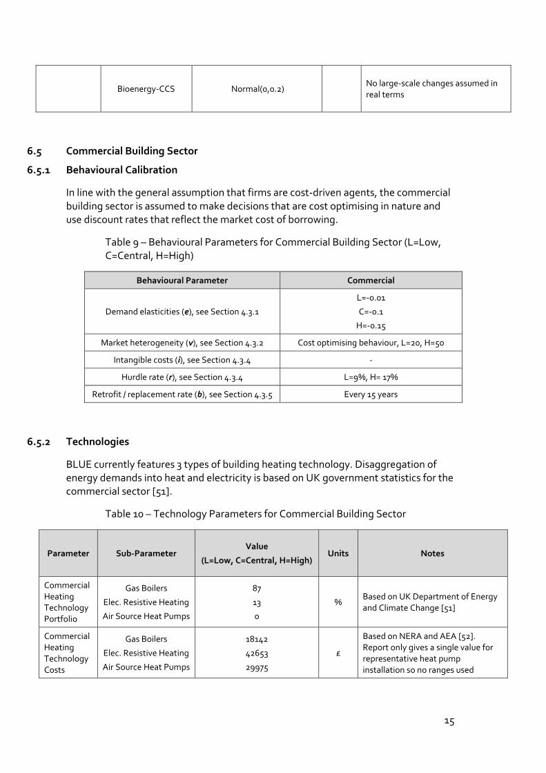
In line with the general assumption that firms are cost-driven agents, the commercial building sector is assumed to make decisions that are cost optimising in nature and use discount rates that reflect the market cost of borrowing.
Table 9 – Behavioural Parameters for Commercial Building Sector (L=Low, C=Central, H=High)
Behavioural Parameter Commercial
Demand elasticities (e), see Section 4.3.1
L=-0.01
C=-0.1
H=-0.15
Market heterogeneity (v), see Section 4.3.2 Cost optimising behaviour, L=20, H=50
Intangible costs (i), see Section 4.3.4 -
Hurdle rate (r), see Section 4.3.4 L=9%, H= 17%
Retrofit / replacement rate (b), see Section 4.3.5 Every 15 years
6.5.2 Technologies
BLUE currently features 3 types of building heating technology. Disaggregation of energy demands into heat and electricity is based on UK government statistics for the commercial sector [51].
Table 10 – Technology Parameters for Commercial Building Sector
Parameter Sub-Parameter Value
(L=Low, C=Central, H=High) Units Notes
Commercial Heating Technology Portfolio
Gas Boilers
Elec. Resistive Heating
Air Source Heat Pumps
87
13
0
% Based on UK Department of Energy and Climate Change [51]
Commercial Heating Technology Costs
Gas Boilers
Elec. Resistive Heating
Air Source Heat Pumps
18142
42653
29975
£
Based on NERA and AEA [52]. Report only gives a single value for representative heat pump installation so no ranges used

16
Commercial Heating Efficiency
Gas Boilers
Elec. Resistive Heating
Air Source Heat Pumps
94
100
350
% Based on NERA and AEA [52]
6.5.3 Default Technological Change Parameters
Future changes to commercial building sector technologies that are assumed by default in the model are shown below, with accompanying references. End-users should explore alternative trajectories for future technological change as they see fit.
Table 11 – Default Technological Change Parameters for Commercial Building Sector
Parameter Sub-Parameter Value
(L=Low, C=Central, H=High) Units Notes
Commercial Heating Annual Technology Cost Change
Gas Boilers
Elec. Resistive Heating
Air Source Heat Pumps
Normal(0,0.2)
Normal(0,0.2)
Triangular(H=-1,C=-0.6,L=-0.3)
%
Gas boilers and electric resistive heating are mature technologies, and the model default assumptions are that there will be no major changes to costs in real terms.
Future cost changes to air source heat pumps are based on studies by Sweett Group / BuroHappold [53] and Frontier Economics / Element Energy [54]
6.6 Residential Building Sector
6.6.1 Behavioural Calibration
The residential building sector is captured using five representative agents which we term innovators, early adopters, early majority, late majority, and laggards. These are set up on a spectrum to be more or less risk-averse. Intangible costs for these agents are expressed as a percentage of the intangible costs described in Section 6.5.2.
Table 12 – Behavioural Parameters for Residential Building Sector (L=Low, C=Central, H=High)
Behavioural Parameter Innovators Early Adopters Early Majority Late Majority Laggards
Demand elasticities (e), see Section 4.3.1
L=-0.1
C=-0.25
H=-0.40

17
Market heterogeneity (v), see Section 4.3.2
Price insensitive, L=0, H=4
Partial price sensitivity, L=5,
H=9
Partial price sensitivity, L=5,
H=9
Strong price sensitivity, L=10, H=19
Cost optimising behaviour, L=20, H=50
Intangible costs (i), see Section 4.3.4
0% 50% 100% 150% 200%
Hurdle rate (r), see Section 4.3.4
3% 5% 10% 15% 20%
Retrofit / replacement rate (b), see Section 4.3.5
Every 15 years
6.6.2 Technologies
The residential sector features similar types of heating technologies to the commercial sector, although the values are different and are drawn from different sources. Disaggregation of energy demands into heat and electricity is based on UK government statistics for the residential [55] sector.
The model does not depict the effect of energy efficiency measures as an output from a complex model that includes important parameters that affect the thermal performance of buildings. Instead, the concept of a highly thermally efficient home (a Near-Zero Heating Home) is included as a stylised heating technology that meets end-use demand for thermal comfort without any fuel costs. Empirical data on the costs of retrofitting existing building to these standards is very sparse, so the model currently uses what could be considered order of magnitude estimates in this regard.
Table 13 – Technology Parameters for Residential Building Sector
Parameter Sub-Parameter Value
(L=Low, C=Central, H=High) Units Notes
Residential Heating Technology Portfolio
Gas Boiler
Elec. Resistive Heating
Air Source Heat Pump
Near-Zero Heating Home
92.8
7.2
0
0
% UK Department of Energy and Climate Change (DECC) [31].
Residential Heating Technology Costs
Gas Boilers
Elec. Resistive Heating
Air Source Heat Pumps
Near-Zero Heating Home
L=2500, H=3000
L=1750, H=4025
L=8400, H=10500
L=60,000, H=100,000
£
Uniform distributions used to span range of estimates for heating [52].
Ex-post analysis of Passivhaus projects in the UK finds that new build costs were around £140,000 [56]. Anecdotal discussion seems to find that retrofit projects are not much cheaper than new build and could be easily in the range of 60,000 - 100,000.

18
Residential Heating
Efficiency
Gas Boilers
Elec. Resistive Heating
Air Source Heat Pumps
Near-Zero Heating Home
94
100
250-275
-
% Based on NERA and AEA [52]
Residential Heating Intangible Costs
Gas Boilers
Elec. Resistive Heating
Air Source Heat Pumps
Near-Zero Heating Home
0
0
L=200, H=480
20,000
£ Heat pumps based on Holdaway et. al [57]
Residential Microgen Technology Portfolio
Residential Photovoltaics 0 % -
Residential Microgen Technology Costs
Residential Photovoltaics L = 5842, C = 6666, H = 7912 £ Based on Parsons Brinckerhoff [58]
Residential Microgen Intangible Costs
Residential Photovoltaics 5000 £ Based on Parsons Brinckerhoff [58] and Scarpa and Willis [59]
6.6.3 Default Technological Change Parameters
Future changes to residential building sector technologies that are assumed by default in the model are shown below, with accompanying references. End-users can modify these numbers as desired to explore alternative trajectories.
Parameter Sub-Parameter Value
(L=Low, C=Central, H=High) Units Notes
Residential Heating Annual Technology Cost Change
Gas Boilers
Elec. Resistive Heating
Normal(0,0.2) Normal(0,0.2)
%
Gas boilers and electric resistive heating are mature technologies, and the model default assumptions are that there will be no major changes to costs in real terms.
Air Source Heat Pumps Triangular(H=-1,C=-0.6,L=-
0.3)
Future cost changes to air source heat pumps are based on studies by Sweett Group / BuroHappold [53] and Frontier Economics / Element Energy [54]
Residential Microgen Annual
Residential Photovoltaics If Time<= 2030 then
Triangular(H=-3.3735,M=-2.5665,L=-1.0144) else 0
% Based on Parsons Brinckerhoff [58]
19
Technology Cost Change
6.7 Industrial Sector
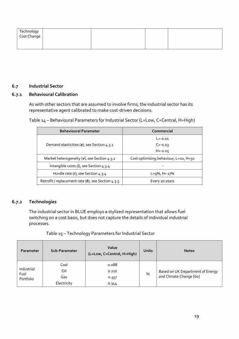
6.7.1 Behavioural Calibration
As with other sectors that are assumed to involve firms, the industrial sector has its representative agent calibrated to make cost-driven decisions.
Table 14 – Behavioural Parameters for Industrial Sector (L=Low, C=Central, H=High)
Behavioural Parameter Commercial
Demand elasticities (e), see Section 4.3.1
L=-0.01
C=-0.03
H=-0.05
Market heterogeneity (v), see Section 4.3.2 Cost optimising behaviour, L=20, H=50
Intangible costs (i), see Section 4.3.4 -
Hurdle rate (r), see Section 4.3.4 L=9%, H= 17%
Retrofit / replacement rate (b), see Section 4.3.5 Every 20 years
6.7.2 Technologies
The industrial sector in BLUE employs a stylized representation that allows fuel switching on a cost basis, but does not capture the details of individual industrial processes.
Table 15 – Technology Parameters for Industrial Sector
Parameter Sub-Parameter Value
(L=Low, C=Central, H=High) Units Notes
Industrial Fuel Portfolio
Coal
Oil
Gas
Electricity
0.088
0.210
0.357
0.344
% Based on UK Department of Energy and Climate Change [60]

20
6.8 Road Transport Sector
6.8.1 Behavioural Calibration
As with residential building sector, the road transport sector is captured using five representative agents: innovators, early adopters, early majority, late majority, and laggards, who have differentiated attitudes to risk and investment that are reflected in their behavioural parameter settings.
Table 16 – Behavioural Parameters for Road Transport Sector (L=Low, C=Central, H=High)
Behavioural Parameter Innovators Early Adopters Early Majority Late Majority Laggards
Demand elasticities (e), see Section 4.3.1
L=-0.15
C=-0.3
H=-0.50
Market heterogeneity (v), see Section 4.3.2
Price insensitive, L=0, H=4
Partial price sensitivity, L=5,
H=9
Partial price sensitivity, L=5,
H=9
Strong price sensitivity, L=10, H=19
Cost optimising behaviour, L=20, H=50
Intangible costs (i), see Section 4.3.4
0% 50% 100% 150% 200%
Hurdle rate (r), see Section 4.3.4
3% 5% 10% 15% 20%
Retrofit / replacement rate (b), see Section 4.3.5
Every 10 years
6.8.2 Technologies
BLUE currently features two types of road vehicle technology – a generic electric drivetrain vehicle and a generic fossil fuel vehicle. A third technology is used to capture the concept of Non-Motorised Transport (NMT) – this is captured as a low-cost vehicle type that has no fuel costs. In order to represent the idea that there are both range constraints for typical trip distances using non-motorised options as well as infrastructural constraints (availability of cycle pathways etc.) the model employs a constraint of 670 pkm/capita for NMT, based on analysis carried out in Pye and Daly [61] aimed at integrated sustainable road travel options into energy system models.
Table 17 – Technology Parameters for Road Transport Sector
Parameter Sub-Parameter Value
(L=Low, C=Central, H=High) Units Notes
Road Transport Technology Portfolio
Fossil Fuel Vehicles
Electric Vehicles
Non-Motorised Transport
100
0
0
%
Electric vehicle sales in the UK were less than 0.1% of annual sales in 2012 [62], so it can be
21
assumed that as a fraction of the road fleet composition they were negligible in 2010.
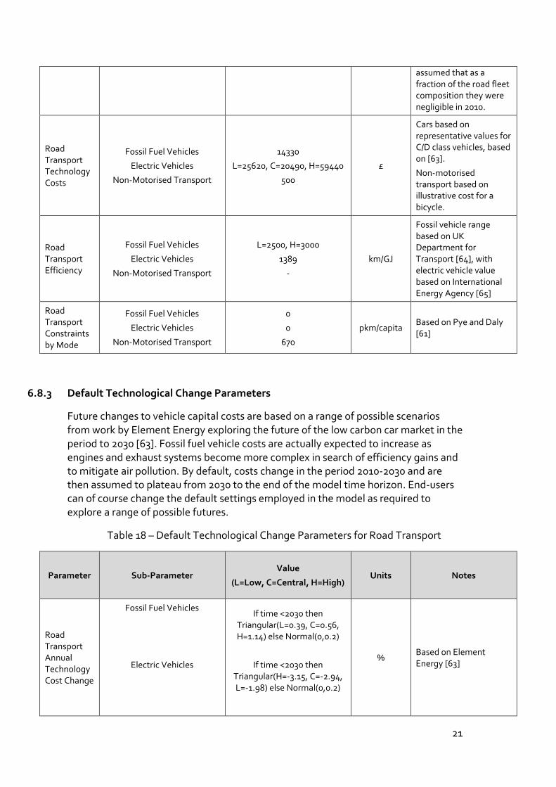
Road Transport Technology Costs
Fossil Fuel Vehicles
Electric Vehicles
Non-Motorised Transport
14330
L=25620, C=20490, H=59440
500
£
Cars based on representative values for C/D class vehicles, based on [63].
Non-motorised transport based on illustrative cost for a bicycle.
Road Transport Efficiency
Fossil Fuel Vehicles
Electric Vehicles
Non-Motorised Transport
L=2500, H=3000
1389
-
km/GJ
Fossil vehicle range based on UK Department for Transport [64], with electric vehicle value based on International Energy Agency [65]
Road Transport Constraints by Mode
Fossil Fuel Vehicles
Electric Vehicles
Non-Motorised Transport
0
0
670
pkm/capita Based on Pye and Daly [61]
6.8.3 Default Technological Change Parameters
Future changes to vehicle capital costs are based on a range of possible scenarios from work by Element Energy exploring the future of the low carbon car market in the period to 2030 [63]. Fossil fuel vehicle costs are actually expected to increase as engines and exhaust systems become more complex in search of efficiency gains and to mitigate air pollution. By default, costs change in the period 2010-2030 and are then assumed to plateau from 2030 to the end of the model time horizon. End-users can of course change the default settings employed in the model as required to explore a range of possible futures.
Table 18 – Default Technological Change Parameters for Road Transport
Parameter Sub-Parameter Value
(L=Low, C=Central, H=High) Units Notes
Road Transport Annual Technology Cost Change
Fossil Fuel Vehicles
Electric Vehicles
If time <2030 then Triangular(L=0.39, C=0.56, H=1.14) else Normal(0,0.2)
If time <2030 then Triangular(H=-3.15, C=-2.94, L=-1.98) else Normal(0,0.2)
% Based on Element Energy [63]

22
Non-Motorised Transport
0
6.9 Other Transport Sectors
6.9.1 Behavioural Calibration
Non-road transport actors in the current model version have very limited decision-making powers as there are not yet explicit technology and fuel switching options. However, the representative agents for each sector are sensitive to changes in fuel prices.
Table 19 – Behavioural Parameters for Other Transport Sectors (L=Low, C=Central, H=High)
Behavioural Parameter Transport
(Air)
Transport
(Rail)
Transport (Marine)
Demand elasticities (e), see Section 4.3.1
L=-0.40
C=-0.70
H=-1.00
L=-0.60
C=-0.80
H=-1.10
L=-0.01
C=-0.03
H=-0.06
Market heterogeneity (v), see Section 4.3.2
- - -
Intangible costs (i), see Section 4.3.4 - - -
Hurdle rate (r), see Section 4.3.4 - - -
Retrofit / replacement rate (b), see Section 4.3.5
- - -
6.9.2 Technologies
The non-road transport sectors have few technological mitigation options in the current model version. Future changes to aviation technologies are captured as reductions in CO2 intensity per unit of energy demand (2% reduction per year from 2010-2050) to reflect efficiency improvements that are likely to arise over the time horizon at zero marginal costs from existing R&D investments [66]. Radical design changes to aircraft and/or air travel infrastructure are not represented. Fuel switching and technological change in the marine and rail sectors is also not presently captured in the current model version. These latter two sectors are currently small in absolute consumption terms, together comprising 3.5% of UK transport energy demand [31].
7.0 History of Model Versions and Associated Publications
It can sometimes be challenging to understand the differences between multiple versions of the same model when it is applied to different studies [1]. This section of

23
the documentation is intended to mitigate this challenge by providing an understanding of which model versions have been used to produce which publications and what the key changes have been between revisions.
7.1 Early Versions
An early development version of the model was calibrated for the city of London, and used to showcase the core concept of a multi-agent transition model in a conference paper titled “Incorporating Behavioural Complexity in Energy-Economic Models” [67]. An early version, without a formal version designation, was calibrated for UK energy balances and featured within a multi-model comparison paper “Linking a storyline with multiple models: A cross-scale study of the UK power system transition” [68].
7.2 Model Version 1.7.1, June 2016
This was the first version of the model that was published alongside a fully documented description of its key feature and inputs. This formed the centrepiece of a journal publication in Environmental Innovation and Societal Transitions on energy transitions modelling, entitled “Modelling energy transitions for climate targets under landscape and actor inertia” [20].
7.3 Model Version 1.9.4_RI, November 2016 – March 2017
This version of the model was used for a single journal publication in Energy Strategy Reviews on decision-making in second-best policy environments called “Actors behaving badly: Exploring the modelling of non-optimal behaviour in energy transitions” [69].
Key changes from previous version include:
Endogenous calculation of Levelised Cost of Energy (LCOE) for the power sector.
Addition of a stylised Bioenergy with Carbon Capture and Storage (BECCS) technology for the power sector.
Introduction of installed capacity constraints for power generation technologies.
7.4 Model Version 2.3, April 2017 – Present
This version of the model was featured in a publication in Energy Research and Social Science: “Take me to your leader: using socio-technical energy transitions (STET) modelling to explore the role of actors in decarbonisation pathways” [70].
Key changes from the previous version include:

24
Model time horizon extended from 2050 to 2070.
Addition of Government as a representative agent with decision-making powers over CO2 prices, incentives for low carbon technologies, penalties for polluting technologies, and regulating technologies out of the options space.
Disaggregation of domestic sector and road transport sector into five stylised societal groups with names drawn from Rogers [15] seminal work on the diffusion of innovations: innovators, early adopters, early majority, late majority, and laggards.
Addition of: domestic microgeneration, non-motorised transport, and highly thermally efficient buildings.
8.0 References
[1] P.E. Dodds, I. Keppo, N. Strachan, Characterising the Evolution of Energy System Models Using Model Archaeology, Environ. Model. Assess. 20 (2015) 83–102. doi:10.1007/s10666-014-9417-3.
[2] A. Voinov, F. Bousquet, Modelling with stakeholders, Environ. Model. Softw. 25 (2010) 1268–1281. doi:10.1016/j.envsoft.2010.03.007.
[3] N. Hughes, N. Strachan, Methodological review of UK and international low carbon scenarios, Energy Policy. 38 (2010) 6056–6065. doi:10.1016/j.enpol.2010.05.061.
[4] M.G. Morgan, M. Henrion, Uncertainty: A Guide to Dealing with Uncertainty in Quantitative Risk and Policy Analysis, Cambridge University Press, 1992. http://www.cambridge.org/jp/academic/subjects/psychology/cognition/uncertainty-guide-dealing-uncertainty-quantitative-risk-and-policy-analysis?format=PB.
[5] S. Pye, C. Bataille, Improving deep decarbonization modelling capacity for developed and developing country contexts, Clim. Policy. 16 (2016) S27–S46. doi:10.1080/14693062.2016.1173004.
[6] C. Bataille, M. Jaccard, J. Nyboer, N. Rivers, Towards General Equilibrium in a Technology-Rich Model with Empirically Estimated Behavioral Parameters, Energy J. SI2006 (2006). doi:10.5547/ISSN0195-6574-EJ-VolSI2006-NoSI2-5.
[7] P. Capros, L. Paroussos, P. Fragkos, S. Tsani, B. Boitier, F. Wagner, S. Busch, G. Resch, M. Blesl, J. Bollen, Description of models and scenarios used to assess European decarbonisation pathways, Energy Strateg. Rev. 2 (2014) 220–230. doi:10.1016/j.esr.2013.12.008.
[8] L. Mantzos, N.A. Matei, M. Rózsai, P. Russ, A.S. Ramirez, POTEnCIA: A new EU-wide energy sector model, in: 2017 14th Int. Conf. Eur. Energy Mark., IEEE, 2017: pp. 1–5. doi:10.1109/EEM.2017.7982028.

25
[9] H. Waisman, C. Guivarch, F. Grazi, J.C. Hourcade, The Imaclim-R model: infrastructures, technical inertia and the costs of low carbon futures under imperfect foresight, Clim. Change. 114 (2012) 101–120. doi:10.1007/s10584-011-0387-z.
[10] K. Hasselmann, D. V. Kovalevsky, Simulating animal spirits in actor-based environmental models, Environ. Model. Softw. 44 (2013) 10–24. doi:10.1016/j.envsoft.2012.04.007.
[11] J.M. Epstein, R.L. Axtell, Growing artificial societies: Social science from the bottom up, Comput. Math. with Appl. 33 (1997) 127. doi:10.1016/S0898-1221(97)82923-9.
[12] L. Börjeson, M. Höjer, K.-H. Dreborg, T. Ekvall, G. Finnveden, Scenario types and techniques: Towards a user’s guide, Futures. 38 (2006) 723–739. doi:10.1016/j.futures.2005.12.002.
[13] J.B. Robinson, Futures under glass, Futures. 22 (1990) 820–842. doi:10.1016/0016-3287(90)90018-D.
[14] I. Keppo, M. Strubegger, Short term decisions for long term problems – The effect of foresight on model based energy systems analysis, Energy. 35 (2010) 2033–2042. doi:10.1016/j.energy.2010.01.019.
[15] E.M. Rogers, Diffusion of Innovations, 5th Editio, Free Press Simon and Schuster, New York, NY, USA, 2003. http://www.simonandschuster.com/books/Diffusion-of-Innovations-5th-Edition/Everett-M-Rogers/9780743222099.
[16] E. Krick, Ensuring social acceptance of the energy transition. The German government’s ‘consensus management’ strategy, J. Environ. Policy Plan. 20 (2018) 64–80. doi:10.1080/1523908X.2017.1319264.
[17] E. Patashnik, After the Public Interest Prevails: The Political Sustainability of Policy Reform, Governance. 16 (2003) 203–234. doi:10.1111/1468-0491.00214.
[18] M. Lockwood, The political sustainability of climate policy: The case of the UK Climate Change Act, Glob. Environ. Chang. 23 (2013) 1339–1348. doi:10.1016/j.gloenvcha.2013.07.001.
[19] S. Pye, W. Usher, N. Strachan, The uncertain but critical role of demand reduction in meeting long-term energy decarbonisation targets, Energy Policy. 73 (2014) 575–586. doi:10.1016/j.enpol.2014.05.025.
[20] F.G.N. Li, N. Strachan, Modelling energy transitions for climate targets under landscape and actor inertia, Environ. Innov. Soc. Transitions. 24 (2017) 106–129. doi:10.1016/j.eist.2016.08.002.
[21] D. Ürge-Vorsatz, A. Novikova, S. Köppel, B. Boza-Kiss, Bottom–up assessment of potentials and costs of CO2 emission mitigation in the buildings sector: insights into the missing elements, Energy Effic. 2 (2009) 293–316.
26
doi:10.1007/s12053-009-9051-0.
[22] H. Pollitt, S. Billington, The Use of Discount Rates in Policy Modelling, Cambridge Econometrics, 2015. http://www.camecon.com/Libraries/Downloadable_Files/The_use_of_Discount_Rates_in_Policy_Modelling.sflb.ashx.
[23] D. Moellendorf, Discounting the Future and the Morality in Climate Change Economics, in: Moral Chall. Danger. Clim. Chang., Cambridge University Press, New York, 2013: pp. 90–122. doi:10.1017/CBO9781139083652.005.
[24] HM Treasury, The Green Book: Appraisal and Evaluation in Central Government, London, UK, 2011. http://www.hm-treasury.gov.uk/d/green_book_complete.pdf.
[25] A.H. Hermelink, D. de Jager, Evaluating our Future: The Crucial Role of Discount Rates in European Commission Energy System Modelling, Ecofys for The European Council for an Energy Efficient Economy (eceee), 2015. http://europeanclimate.org/evaluating-our-future-the-crucial-role-of-discount-rates-in-european-commission-energy-system-modelling/.
[26] L. Schrattenholzer, The Energy Supply Model MESSAGE, International Institute for Applied Systems Analysis (IIASA), Laxenburg, Austria, 1981. http://webarchive.iiasa.ac.at/Publications/Documents/RR-81-031.pdf.
[27] R. Loulou, G. Goldstein, A. Kanudia, A. Lehtila, U. Remme, Documentation for the TIMES Model; Part 1 TIMES concepts and theory, Energy Technology Systems Analysis Programme (ETSAP), 2016. https://iea-etsap.org/docs/Documentation_for_the_TIMES_Model-Part-I_July-2016.pdf.
[28] M. Howells, H. Rogner, N. Strachan, C. Heaps, H. Huntington, S. Kypreos, A. Hughes, S. Silveira, J.F. DeCarolis, M. Bazillian, A. Roehrl, OSeMOSYS: The Open Source Energy Modeling System, Energy Policy. 39 (2011) 5850–5870. doi:10.1016/j.enpol.2011.06.033.
[29] R.J. Sutherland, Market Barriers to Energy-Efficiency Investments, Energy J. 12 (1991). doi:10.5547/ISSN0195-6574-EJ-Vol12-No3-3.
[30] J. Nyober, Simulating Evolution of Technology: An Aid to Energy Policy Analysis, Simon Fraser University, 1997. http://www.collectionscanada.gc.ca/obj/s4/f2/dsk3/ftp04/nq24339.pdf.
[31] DECC, Energy consumption in the United Kingdom: 2011 - Overall energy consumption in the UK since 1970 (Publication URN 11D/806), UK Department of Energy and Climate Change (DECC), London, UK, 2011.
[32] ONS, National Population Projections, 2012-based Statistical Bulletin, UK Office of National Statistics (ONS), Newport, UK, 2013. http://www.ons.gov.uk/ons/dcp171778%7B_%7D334975.pdf.
[33] DECC, DECC Fossil Fuel Price Projections, July 2013 (URN 13D/170),

27
Department of Energy and Climate Change (DECC), London, UK, 2013. https://www.gov.uk/government/uploads/system/uploads/attachment_data/file/212521/130718_decc-fossil-fuel-price-projections.pdf.
[34] EIA, Annual Energy Review 2011: DOE/EIA-0384(2011), United States Energy Information Administration (EIA), Washington D.C., USA, 2012. https://www.eia.gov/totalenergy/data/annual/pdf/aer.pdf.
[35] Parsons Brinckerhoff, Electricity Generation Cost Model - 2011 Update, 2011. http://www.decc.gov.uk/assets/decc/11/meeting-energy-demand/nuclear/2153-electricity-generation-cost-model-2011.pdf.
[36] Parsons Brinckerhoff, Electricity Generation Costs Model: 2013 Update of Renewable Technologies, Parsons Brinckerhoff, Newcastle, UK, 2013. https://www.gov.uk/government/publications/parsons-brinkerhoff-electricity-generation-model-2013-update-of-renewable-technologies.
[37] E. de Visser, A. Held, Methodologies for estimating Levelised Cost of Electricity (LCOE), 2014. http://res-cooperation.eu/images/pdf-reports/ECOFYS_Fraunhofer_Methodologies_for_estimating_LCoE_Final_report.pdf.
[38] DECC, Digest of United Kingdom Energy Statistics (DUKES) 2015, Department of Energy and Climate Change (DECC), London, UK, 2015. https://www.gov.uk/government/statistics/digest-of-united-kingdom-energy-statistics-dukes-2015-printed-version.
[39] G. Harris, P. Heptonstall, R. Gross, D. Handley, Cost estimates for nuclear power in the UK, ICEPT Working Paper (ICEPT/WP/2012/014), Imperial College Centre for Energy Policy and Technology (ICEPT), London, UK, 2012. https://workspace.imperial.ac.uk/icept/Public/Cost.
[40] DECC, Renewables Obligation Banding Review for the period 1 April 2013 to 31 March 2017: Government Response to further consultations on solar PV support, biomass affordability and retaining the minimum calorific value requirement in the RO, 2012. https://www.gov.uk/government/uploads/system/uploads/attachment_data/file/66516/7328-renewables-obligation-banding-review-for-the-perio.pdf.
[41] SKM, Quantification of Constraints on the Growth of UK Renewable Generating Capacity, Sinclair Knight Merz (SKM), Newcastle upon Tyne, UK, 2008. https://www.gov.uk/government/uploads/system/uploads/attachment_data/file/42966/1_20090501131320_e____SKMRenewableConstraintsReportFinal425062008.pdf.
[42] The Offshore Valuation Group, The Offshore Valuation, Department of Energy & Climate Change, Scottish Government, Welsh Assembly Government, Crown Estate, Energy Technologies Institute, Scottish & Southern Energy, RWE Innogy, E.ON, DONG Energy, Statoil, Mainstream Renewable Power, RES,

28
Vestas, PIRC, 2010. http://publicinterest.org.uk/offshore/.
[43] CCC, Bioenergy Review, The Committee on Climate Change (CCC), London, UK, 2011. http://www.theccc.org.uk/reports/bioenergy-review.
[44] CCC, Bioenergy Review: Technical Paper 2: Global and UK Bioenergy Supply Scenarios, The Committee on Climate Change (CCC), London, UK, 2011. http://archive.theccc.org.uk/aws2/Bioenergy/1463.
[45] Royal Academy of Engineering, GB electricity capacity margin, The Royal Academy of Engineering, London, UK, 2013. https://www.gov.uk/government/publications/electricity-capacity-margin-report.
[46] Ofgem, Electricity Capacity Asessment Report 2013, Office of Gas and Electricity Markets (Ofgem), London, UK, 2013. https://www.ofgem.gov.uk/ofgem-publications/75232/electricity-capacity-assessment-report-2013.pdf.
[47] J. Hemingway, Special feature – FiT generation methodology: Estimating generation from Feed in Tariff installations, Department of Energy and Climate Change (DECC), London, UK, 2013. https://www.gov.uk/government/uploads/system/uploads/attachment_data/file/266474/estimating_generation_from_fit_installations.pdf.
[48] J. Chapman, W. Goldthorpe, J. Overton, P. Dixon, P. Hare, S. Murray, The potential for reducing the costs of CCS in the UK: Interim Report of the UK Carbon Capture and Storage Cost Reduction Task Force, London, UK, 2012. https://www.gov.uk/government/uploads/system/uploads/attachment%7B_%7Ddata/file/198823/ccsa%7B_%7Dctrf%7B_%7Dinterim%7B_%7Dreport.pdf.
[49] DECC, Electricity Generation Costs (December 2013) URN 14D/005, UK Department of Energy and Climate Change (DECC), London, UK, 2013. https://www.gov.uk/government/uploads/system/uploads/attachment%7B_%7Ddata/file/269888/131217%7B_%7DElectricity%7B_%7DGeneration%7B_%7Dcosts%7B_%7Dreport%7B_%7DDecember%7B_%7D2013%7B_%7DFinal.pdf.
[50] The Crown Estate, Offshore Wind Cost Reduction Pathways Study, The Crown Estate, London, UK, 2012. http://www.thecrownestate.co.uk/media/5493/ei-offshore-wind-cost-reduction-pathways-study.pdf.
[51] DECC, Energy consumption in the United Kingdom (2015): Chapter 5 - Service sector energy consumption in the UK between 1970 and 2014 (Publication URN 15D/381), Department of Energy and Climate Change (DECC), London, UK, 2015. https://www.gov.uk/government/statistics/energy-consumption-in-the-uk.
[52] NERA, AEA, The UK Supply Curve for Renewable Heat: Study for the Department of Energy and Climate Change, Department of Energy and Climate Change (DECC), London, UK, 2009.

29
http://www.rhincentive.co.uk/library/regulation/0907Heat_Supply_Curve.pdf.
[53] Sweett Group, Buro Happold, ACE, Research on the costs and performance of heating and cooling technologies, 2013. https://www.gov.uk/government/consultations/non-domestic-rhi-early-tariff-review.
[54] Frontier Economics, Element Energy, Pathways to high penetration of heat pumps, Frontier Economics and Element Energy for the Committee on Climate Change (CCC), London, UK, 2013. http://www.theccc.org.uk/wp-content/uploads/2013/12/Frontier-Economics-Element-Energy-Pathways-to-high-penetration-of-heat-pumps.pdf.
[55] DECC, Energy consumption in the United Kingdom (2015): Chapter 3 - Domestic energy consumption in the UK between 1970 and 2014 (Publication URN 15D/377), Department of Energy and Climate Change (DECC), London, UK, 2015. https://www.gov.uk/government/statistics/energy-consumption-in-the-uk.
[56] Passivhaus Trust & AECOM, Passivhaus Capital Cost Research Project, Passivhaus Trust, London, UK, 2015. http://www.passivhaustrust.org.uk/news/detail/?nId=638.
[57] E. Holdaway, B. Samuel, J. Greenleaf, A. Briden, A. Gardiner, The Hidden Costs and Benefits of Domestic Energy Efficiency and Carbon Saving Measures, Ecofys for Department of Energy and Climate Change (DECC), 2009. http://www.decc.gov.uk/assets/decc/whatwedo/supportingconsumers/saving_energy/analysis/1_20100111103046_e_@@_ecofyshiddencostandbenefitsdefrafinaldec2009.pdf.
[58] P. Brinckerhoff, Solar PV Cost Update, 2012. https://www.gov.uk/government/uploads/system/uploads/attachment%7B_%7Ddata/file/43083/5381-solar-pv-cost-update.pdf.
[59] R. Scarpa, K. Willis, Willingness-to-pay for renewable energy: Primary and discretionary choice of British households’ for micro-generation technologies, Energy Econ. 32 (2010) 129–136. doi:10.1016/j.eneco.2009.06.004.
[60] DECC, Energy consumption in the United Kingdom (2015): Chapter 4 - Industrial energy consumption in the UK between 1970 and 2014 (Publication URN 15D/379), Department of Energy and Climate Change (DECC), London, UK, 2015. https://www.gov.uk/government/statistics/energy-consumption-in-the-uk.
[61] S. Pye, H. Daly, Modelling sustainable urban travel in a whole systems energy model, Appl. Energy. 159 (2015) 97–107. doi:10.1016/j.apenergy.2015.08.127.
[62] Element Energy, Pathways to high penetration of electric vehicles: Final report for the Committee on Climate Change, Element Energy, Cambridge, UK, 2013. http://www.theccc.org.uk/wp-content/uploads/2013/12/CCC-EV-

30
pathways_FINAL-REPORT_17-12-13-Final.pdf.
[63] Element Energy, Influences on the Low Carbon Car Market from 2020-2030: Final Report for Low Carbon Vehicle Partnership, Element Energy, Cambridge, UK, 2011. lowcvp.org.uk/assets/reports/Influences.
[64] DfT, Average new car fuel consumption: Great Britain (Table ENV0103), UK Department for Transport (DfT), London, UK, 2014. https://www.gov.uk/government/statistical-data-sets/env01-fuel-consumption.
[65] IEA, Technology Roadmap: Electric and plug-in hybrid electric vehicles, International Energy Agency (IEA), Paris, France, 2011. https://www.iea.org/publications/freepublications/publication/EV_PHEV_Roadmap.pdf.
[66] A.W. Schäfer, A.D. Evans, T.G. Reynolds, L. Dray, Costs of mitigating CO2 emissions from passenger aircraft, Nat. Clim. Chang. 6 (2015) 412–417. doi:10.1038/nclimate2865.
[67] N. Strachan, P. Warren, Incorporating Behavioural Complexity in Energy-Economic Models, in: UK Energy Res. Cent. Conf. Energy People Futur. Complex. Challenges, Environmental Change Institute, Oxford, UK, 2011: pp. 1–20.
[68] E. Trutnevyte, J. Barton, Á. O’Grady, D. Ogunkunle, D. Pudjianto, E. Robertson, Linking a storyline with multiple models: A cross-scale study of the UK power system transition, Technol. Forecast. Soc. Change. 89 (2014) 26–42. doi:10.1016/j.techfore.2014.08.018.
[69] F.G.N. Li, Actors behaving badly: Exploring the modelling of non-optimal behaviour in energy transitions, Energy Strateg. Rev. 15 (2017) 57–71. doi:10.1016/j.esr.2017.01.002.
[70] F.G.N. Li, N. Strachan, Take me to your leader: Using socio-technical energy transitions (STET) modelling to explore the role of actors in decarbonisation pathways, Energy Res. Soc. Sci. 51 (2019) 67–81. doi:10.1016/j.erss.2018.12.010.