Embed Size (px)
Citation preview

Block-Structured Adaptive MeshRefinement
Lecture 3Incompressible AMR
Linear solversMultiphysics applications
– LMC (Low Mach Number Combustion)– AMAR (Adaptive Mesh and Algorithm Refinement)
Short Course Bell 3 – p. 1/44
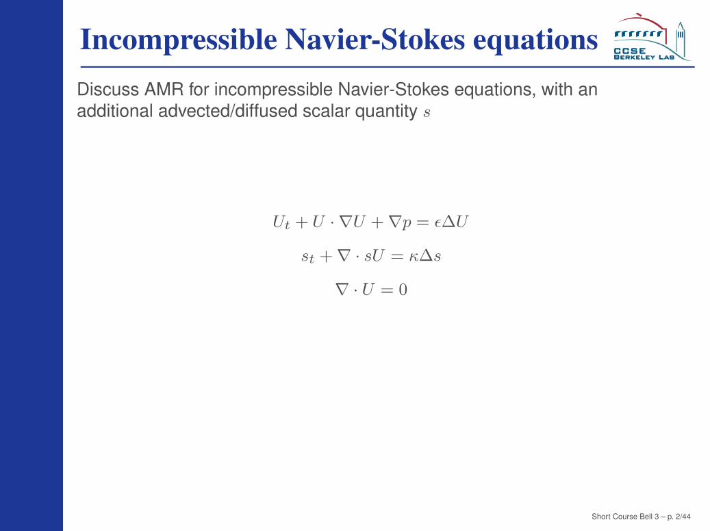
Incompressible Navier-Stokes equationsDiscuss AMR for incompressible Navier-Stokes equations, with anadditional advected/diffused scalar quantity s
Ut + U · ∇U + ∇p = ε∆U
st + ∇ · sU = κ∆s
∇ · U = 0
Short Course Bell 3 – p. 2/44

Review of projection methodFractional step scheme
Advection / Diffusion step:
U∗ − Un
∆t= −[UADV · ∇U ]n+ 1
2 −∇pn− 1
2 + ε∆Un + U∗
2
sn+1 − sn
∆t+ [∇ · sU ]n+1/2 = κ∆
sn + sn+1
2
Projection step:
Solve Lpn+ 1
2 = DV where V = U∗
∆t + Gpn− 1
2
and set
Un+1 = ∆t(V − Gpn+ 1
2 )
Short Course Bell 3 – p. 3/44
Algorithm components
Construction of explicit hyperbolic advection terms for U and s
Cell-centered elliptic solve to enforce constraint at half-time level
Crank-Nicolson discretization of diffusion
Nodal projection to enforce constraint
Short Course Bell 3 – p. 4/44

AMR for projection methodGoal: Combine basic methodology for solving hyperbolic,
parabolic and elliptic PDE’s on hierarchicallyrefined grids to develop efficient adaptiveprojection algorithm
Design Issues: Desireable properties of the adaptive projection algorithm
Second-order accurate in both space and time
Use subcycling in time (i.e. ∆tc = r∆tf )
Conservative“Free-stream” preserving (i.e. constant fields stay constant)
Short Course Bell 3 – p. 5/44

Adaptive projection time stepAdvance (level `)
Predict normal velocitiesDo MAC projection to define advection velocities
Compute advection terms for U, s, etc., using upwind methodology
Solve for diffusive transport using Crank-Nicholson discretization
Perform nodal projection to enforce divergence constraint
if (` < `max)
– Advance(` + 1) r times using Dirichlet boundary conditions fromlevel ` at coarse / fine boundary
– Synchronize levels ` and ` + 1
Short Course Bell 3 – p. 6/44

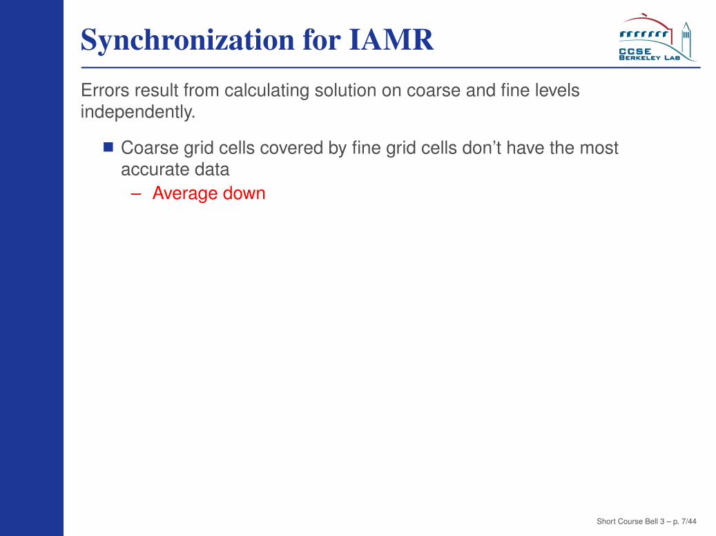
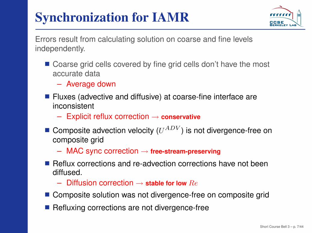
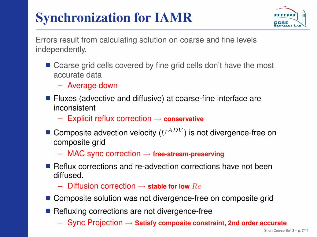
Synchronization for IAMRErrors result from calculating solution on coarse and fine levelsindependently.
Coarse grid cells covered by fine grid cells don’t have the mostaccurate data
– Average down
Fluxes (advective and diffusive) at coarse-fine interface areinconsistent
– Explicit reflux correction → conservative
Composite advection velocity (UADV ) is not divergence-free oncomposite grid
– MAC sync correction → free-stream-preserving
Reflux corrections and re-advection corrections have not beendiffused.
– Diffusion correction → stable for low Re
Composite solution was not divergence-free on composite grid
Refluxing corrections are not divergence-free– Sync Projection → Satisfy composite constraint, 2nd order accurate
Short Course Bell 3 – p. 7/44
Synchronization for IAMRErrors result from calculating solution on coarse and fine levelsindependently.
Coarse grid cells covered by fine grid cells don’t have the mostaccurate data
– Average down
Fluxes (advective and diffusive) at coarse-fine interface areinconsistent
– Explicit reflux correction → conservative
Composite advection velocity (UADV ) is not divergence-free oncomposite grid
– MAC sync correction → free-stream-preserving
Reflux corrections and re-advection corrections have not beendiffused.
– Diffusion correction → stable for low Re
Composite solution was not divergence-free on composite grid
Refluxing corrections are not divergence-free
– Sync Projection → Satisfy composite constraint, 2nd order accurate
Short Course Bell 3 – p. 7/44
Synchronization for IAMRErrors result from calculating solution on coarse and fine levelsindependently.
Coarse grid cells covered by fine grid cells don’t have the mostaccurate data
– Average down
Fluxes (advective and diffusive) at coarse-fine interface areinconsistent
– Explicit reflux correction → conservative
Composite advection velocity (UADV ) is not divergence-free oncomposite grid
– MAC sync correction → free-stream-preserving
Reflux corrections and re-advection corrections have not beendiffused.
– Diffusion correction → stable for low Re
Composite solution was not divergence-free on composite grid
Refluxing corrections are not divergence-free– Sync Projection → Satisfy composite constraint, 2nd order accurate
Short Course Bell 3 – p. 7/44

Explicit RefluxThis step is analogous to the hyperbolic case. Form
δFU = FfU − Fc
U
δFs = Ffs − Fc
s
where these include both advective and diffusive fluxes
For updating s we define
ssync = ∆tc/∆xcδFs
As in the hyperbolic reflux, ssync is only nonzero of coarse cells borderingthe fine grid
Analogously for the velocity we define
V sync = ∆tc/∆xcδFU
These corrections are what is needed to make the scheme conservative.
Short Course Bell 3 – p. 8/44
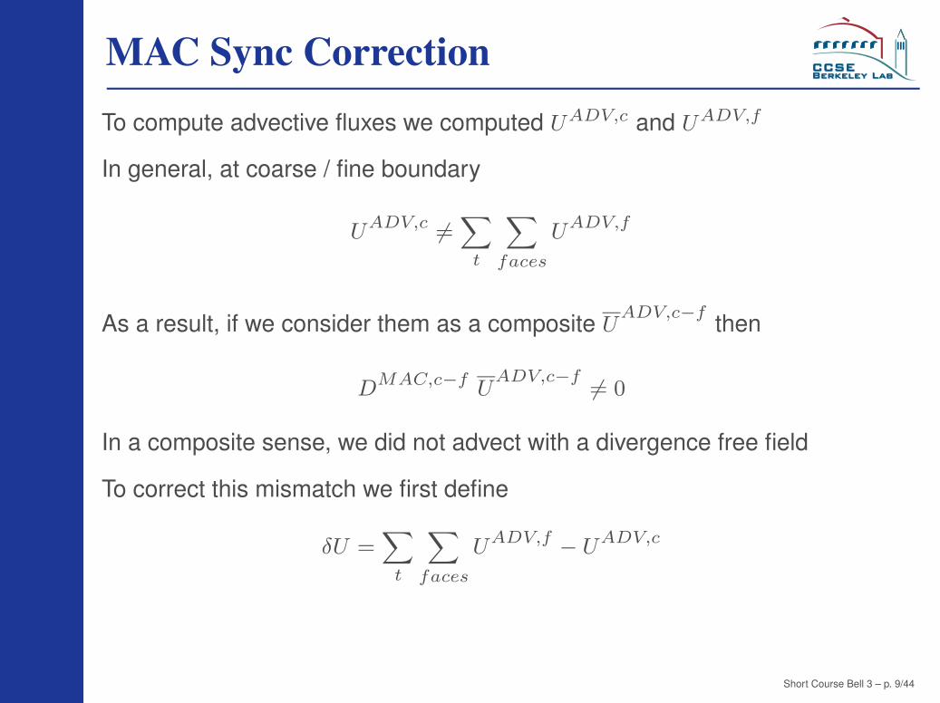
MAC Sync CorrectionTo compute advective fluxes we computed UADV,c and UADV,f
In general, at coarse / fine boundary
UADV,c 6=∑
t
∑
faces
UADV,f
As a result, if we consider them as a composite UADV,c−f then
DMAC,c−f UADV,c−f
6= 0
In a composite sense, we did not advect with a divergence free field
To correct this mismatch we first define
δU =∑
t
∑
faces
UADV,f − UADV,c
Short Course Bell 3 – p. 9/44

MAC Sync Correction (p2)From δU we compute a correction U corr to the composite advectionvelocity by solving
DMACGMACecorr = DMAC(δU)
Ucorr = −Gecorr
and explicitly re-advecting with this “correction velocity”
Namely, we compute
(Ucorr · ∇)U and DMACF corrs = ∇ · (Ucorrs)
These corrections are defined at every coarse grid cell and interpolated tofiner grids
We add these correction to the reflux corrections
ssync : = ssync + ∆tDMACF corrs
V sync : = V sync + ∆t(Ucorr · ∇)U
If κ = 0, sn+1 = sn+1 + ssync synchronizes s Short Course Bell 3 – p. 10/44

MAC Sync Correction (p3)What does this correction do?
Consider the case with s = 1 throughout the domain at tn.
Then sn+ 1
2 = 1 at all edges at tn+ 1
2 , and the correct solution issc,n+1 = sf,n+1 = 1.
But explicit refluxing would replace the value sc,n+1 = 1 (computed duringthe coarse advance) by sc,n+1 = 1 + ∆tc/∆xcδFs.
As a result, the correction to make the scheme conservative introducesspurious variation in s
The MAC sync correction removes this variation:
sn+1 := sn+1 + ∆tc/∆xcδFs + ∆tDMACF corrs ≡ 1
in our example
This makes the scheme free-stream preserving
Short Course Bell 3 – p. 11/44

Diffusing the correctionWhen viscosity/diffusivity is non-zero:
Recall the parabolic synchronization step from the 1-d example.
Instead of adding the refluxing corrections directly to the solution, we mustsolve
(I −ε∆t
2∆h)en+1
U =∆tc
∆xc(δFU ) + ∆tcDMAC(Fcorr
U )(Ucorr · ∇)U ≡ V sync
(I −κ∆t
2∆h)en+1
s =∆tc
∆xc(δFs) + ∆tcDMAC(Fcorr
s ) ≡ ssync
This keeps the scheme stable at low Re.
Thensn+1 := sn+1 + en+1
s
Here we perform a coarse level solve and interpolate to finer grids
We still are not ready to update UShort Course Bell 3 – p. 12/44

Sync ProjectionRemaining problem:
Composite solution was not divergence-free on composite grid
Corrections due to refluxing, etc, are not divergence-free
These mismatches can be combined in the solution of
DGφSP = RHSelliptic + RHSreflux
RHSelliptic = contribution to Dc(Ut − Gφ)c coming from coarse side+∑
time contribution from Df (Ut − Gφ)f coming from fine side
and is non-zero only at coarse nodes on coarse-fine interface
RHSreflux = D(en+1U ) is defined at all nodes with contributions from all
coarse grid cells
Then
pn+1/2,c := pn+1/2,c + φSP
pn+3/4,f := pn+3/4,f + φSP
Un+1,c := Un+1,c − GφSP
Un+1,f := Un+1,f − GφSPShort Course Bell 3 – p. 13/44

Examples
2D shear layer
3D planar jet
Short Course Bell 3 – p. 14/44
Additional software support for IAMRWhat operations must be supported for IAMR that did not exist forhyperbolic AMR?
Linear solvers for parabolic and elliptic equations.
Single-level solvers
Multi-level solvers
Cell-centered (for MAC and diffusive solves)
Node-centered (for projection)
Short Course Bell 3 – p. 15/44
Linear Solvers
Even for single-level solvers, the distribution of points on multiplegrids results in irregular data layout.
Off-the-shelf and black box methods have been inadequate
Iterative methods have proven to be the most efficient solvers.
Multigrid methods, in particular, are desirable– Multigrid naturally respects the AMR hierarchy present in
multi-level solves– Typically require many fewer iterations than other iterative
methods (conjugate gradient)
– O(N log N) as opposed to O(N2)
Short Course Bell 3 – p. 16/44

Multigrid : IntroductionMultigrid is an iterative method in which a multigrid hierarchy ofsuccessively coarser (by a factor of 2) levels is created and each iteration,starting at the level where the problem is specified, recursively calls
MG(m)
smooth the data at level m
if m is not the coarsest level– coarsen the residual data to level m − 1
– call MG(m − 1)– interpolate the corrected coarse data back to level m
smooth the data at level m
This recursive coarsening to the coarsest level then interpolation back tothe finest level is known as a V-cycle.
� � � � � � � �� � � � � � � ���
��
��
��
�
�� �
� � �
�� �
�� �
��
Short Course Bell 3 – p. 17/44

Multigrid for AMRWe distinguish between AMR levels, where we require a solution to theproblem, and multigrid levels, which exist only to facilitate the solution ofthe linear system.
Dotted lines show AMR levels, other levels are used only by multigrid.
Note that multigrid levels can exist between AMR levels if r = 4.
Multiple-AMR-level V-cycle
�� �� �
�� �
� � �
� � �
� �� � � � � � � �� � � � � � � � � �� � � � � �� � � �� � � �
� � � �� ���
��
��
��
��
��
��
��
�
Short Course Bell 3 – p. 18/44
Multigrid: Implementation IssuesMultigrid operations and AMR operations use comparable inter-leveloperations, such as interpolation and restriction.
Because a single solve requires multiple iterations and each iterationrequires significant inter-grid and inter-level communication, multigridmethods are problematic in parallel computing environments: naiveimplementations result in excessive message passing.
– Specialized restriction and interpolation operations are used,since there is a one-to-one correspondence between fine gridsand coarse grids;
– the coarsening of each fine grid can be put on the sameprocessor as the fine grid itself, resulting in locality for restrictionand interpolation.
For single level solves, the degree of coarsening that can be achievedwithin a multigrid V-cycle is limited by the smallest grid. Overallefficiency dictates that grids for IAMR calculations be divisible bymultiple factors of 2. This can be achieved using a blocking-factorrequirement during regridding.
Short Course Bell 3 – p. 19/44

Load Balance for Data LocalityRecall that a Knapsack algorithm can be used for dynamicload-balancing in AMR calculations
– effectively balances computational work across processors– often results in excessive off-processor communications
Can improve communication while maintaining load balance– grids of the same size on different processors are exchanged if
communication is improved.
Initial grid distribution Grid distribution for datalocality
Short Course Bell 3 – p. 20/44

Multiphysics applicationsShock physics
Incompressible flow
MHDRadiation Hydrodynamics
Compressible Navier Stokes
Low mach number modelsCombustionNuclear flamesAtmospheric flows
Biology
Multiphase flow
Porous media flowHybrid methods
Short Course Bell 3 – p. 21/44

Low Mach Number CombustionLow Mach number model, M = U/c � 1 (Rehm & Baum 1978, Majda &Sethian 1985)
Start with the compressible Navier-Stokes equations for multicomponentreacting flow, and expand in the Mach number, M = U/c.
Asymptotic analysis shows that:
p(~x, t) = p0(t) + π(~x, t) where π/p0 ∼ O(M2)
p0 does not affect local dynamics, π does not affect thermodynamics
For open containers p0 is constant
Acoustic waves analytically removed (or, have been “relaxed” away)
Short Course Bell 3 – p. 22/44

Low Mach number combustion
Momentum ρDU
Dt= −∇π + ∇ ·
[
µ
(
∂Ui
∂xj+
∂Uj
∂xi−
2
3δij∇ · U
)]
Species∂(ρYm)
∂t+ ∇ · (ρUYm) = ∇ · (ρDm∇Ym) + ωm
Mass∂ρ
∂t+ ∇ · (ρU) = 0
Energy∂ρh
∂t+ ∇ ·
(
ρh~U)
= ∇ · (λ∇T ) +∑
m
∇ · (ρhmDm∇Ym)
Equation of state p0 = ρRT∑
mYm
Wm
System contains four evolution equations for U, Ym, ρ, h, with a constraintgiven by the EOS.
Short Course Bell 3 – p. 23/44

Constraint for reacting flowsWe differentiate the EOS along particle paths and use the evolutionequations for ρ and T to define a constraint on the velocity:
∇ · U =1
ρ
Dρ
Dt= −
1
T
DT
Dt−
R
R
∑
m
1
Wm
DYm
Dt
=1
ρcpT
(
∇ · (λ∇T ) +∑
m
ρDm∇Ym · ∇hm
)
+
1
ρ
∑
m
W
Wm∇(Dmρ∇Ym) +
1
ρ
∑
m
(
W
Wm−
hm(T )
cpT
)
˙ωm
≡ S
Constraint expresses compressibiity arising from thermal processes
Short Course Bell 3 – p. 24/44

Variable coefficient projectionGeneralized vector field decomposition
V = Ud +1
ρ∇φ
where ∇ · Ud = 0 and U · n = 0 on the boundary
Then Ud and 1ρ∇φ are orthogonal in a density weighted space.
∫
1
ρ∇φ · U ρ dx = 0
Defines a projection Pρ = I − 1ρ∇((∇ · 1
ρ∇)−1)∇· such that PρV = Ud.
Pρ is idempotent and ||Pρ|| = 1
Short Course Bell 3 – p. 25/44

Variable coefficient projection methodWe can use this projection to define a projection scheme for the variabledensity system
ρt + ∇ · ρU = 0
Ut + U · ∇U +1
ρ∇π = 0
∇ · U = 0
Advection stepρn+1 = ρn − ∆t∇ · ρU
U∗ = Un − ∆t U∇ · U1
ρ− ∆t∇πn−1/2
Projection stepUn+1 = PρU∗
Recasts system as initial value problem
Ut + Pρ(U · ∇U) = 0
Short Course Bell 3 – p. 26/44
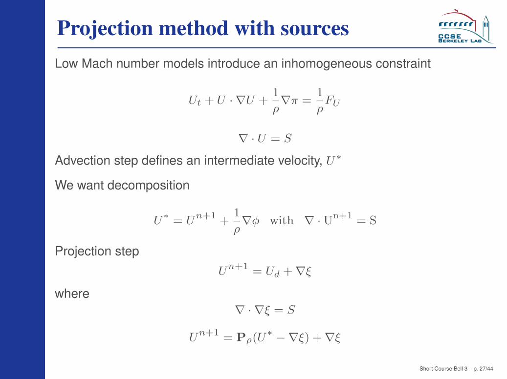
Projection method with sourcesLow Mach number models introduce an inhomogeneous constraint
Ut + U · ∇U +1
ρ∇π =
1
ρFU
∇ · U = S
Advection step defines an intermediate velocity, U∗
We want decomposition
U∗ = Un+1 +1
ρ∇φ with ∇ · Un+1 = S
Projection stepUn+1 = Ud + ∇ξ
where∇ · ∇ξ = S
Un+1 = Pρ(U∗ −∇ξ) + ∇ξ
Short Course Bell 3 – p. 27/44

Fractional Step Approach1. Advance velocity from ~Un to ~Un+1,∗ using explicit advection terms,
Crank-Nicolson diffusion, and a lagged pressure gradient.
2. Update the species and enthalpy equations
3. Use the updated values to compute Sn+1
4. Decompose ~Un+1,∗ to extract the component satisfying thedivergence constraint.
This decomposition is achieved by solving
∇ ·
(
1
ρ∇φ
)
= ∇ ·
(
~Un+1,∗
∆t+
1
ρ∇πn−1/2
)
− Sn+1
for φ, and setting πn+1/2 = φ and
~Un+1 = ~Un+1,∗ −∆t
ρ∇φ
Exploits linearity to represent the compressible component of the velocityShort Course Bell 3 – p. 28/44

Species equation advance
∂(ρYm)
∂t+ ∇ · (ρUYm) = ∇ · (ρDm∇Ym) + ωm
∂(ρh)
∂t+ ∇ · (ρUh) = ∇ · (λ∇T ) +
∑
m
∇ · (ρhmDm∇Ym)
Stiff kinetics relative to fluid dynamical time scales
Operator split approach
Chemistry ⇒ ∆t/2
Advection – Diffusion ⇒ ∆t
Chemistry ⇒ ∆t/2
Short Course Bell 3 – p. 29/44

Properties of the methodologyOverall operator-split projection formulation is 2nd-order accurate in spaceand time.
Godunov-type discretization of advection terms provides a robust2nd-order accurate treatment of advective transport.
Formulation conserves species, mass and energy.
Equation of state is only approximately satisfied
po 6= ρRT∑
m
Ym
Wm
but modified constraint minimizes drift from equation of state.
Short Course Bell 3 – p. 30/44

Model problems
2-D Vortex flame interactions(28th International Combustion Sympsium, 2000)
1.2 × 4.8 mm domain32 species, 177 reactions
3-D Turbulent flame sheet(29th International Combustion Sympsium, 2002)
.8 × .8 × 1.6 cm domain20 species, 84 reactions
0.8 x 0.8 x 1.6 cm domain of
Turbulent Flame Sheet
1.2 x 4.8 cm domain ofVortex-Flame Calculation
Rod-stabilized Flame
Photo courtesy R. Cheng/M. Johnson
5 cm
Laboratory-scale V-flame(19th International Colloquium on the Dynamics of Explosions and Reactive Systems, 2003)
12 × 12 × 12 cm domain20 species, 84 reactions
Short Course Bell 3 – p. 31/44
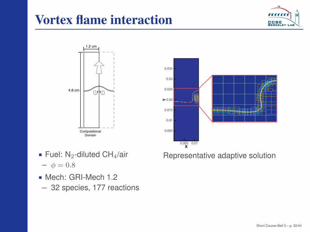
Vortex flame interaction
1.2 cm
4.8 cm
Computational
Domain
Fuel: N2-diluted CH4/air– φ = 0.8
Mech: GRI-Mech 1.2– 32 species, 177 reactions
X
Y
0.005 0.01
0.005
0.01
0.015
0.02
0.025
0.03
0.035
Representative adaptive solution
Short Course Bell 3 – p. 32/44

Convergence Behavior
Vertical Position [m]0.02 0.021 0.022 0.023 0.024
0
2E-08
4E-08
6E-08
8E-08
1E-07
1.2E-07
1.4E-07
1.6E-07
1.8E-07
∆ = 250∆ = 125∆ = 62.5∆ = 31.25
.008 m
.04 m
ComputationalDomain
XCH Along Vortex Centerline
Coarse Fine Finer Finest
Short Course Bell 3 – p. 33/44

Configuration
Burner assembly
190
78
103
130
217
50.8
Settling
Perforated Plate
Swirler
Swirl air injectors
Chamber
Air jetsinclined 20o
Swirler (top view)
CH4/air
Experiment schematic
V-flame (mair ≡ 0): rod ∼ 1 mm
Turbulence plate: 3 mm holes on 4.8 mm center
Short Course Bell 3 – p. 34/44

V-flame Setup
Strategy - Treat nozzle exit asinflow boundary condition forcombustion simulation
Air
Fuel + Air
Flame Zone
(low Mach model)
Nozzle Flow
12cm x 12cm x 12cm domainDRM-19: 20 species, 84
reactionsMixture model for differential
diffusion
Inflow characteristicsMean flow
3 m/s mean inflowBoundary layer profile at edgeNoflow condition to model rodWeak co-flow air
Turbulent fluctuations`t = 3.5mm, u′ = 0.18m/sec
Slightly anisotropic (axial >radial)
Estimated η = 220µm
Use synthetic turbulence fieldshaped to match nozzle flowcharacteristics to specify turbulentfluctuations
Short Course Bell 3 – p. 35/44

Results: Computation vs. Experiment
CH4 from simulation Single image fromexperimental PIV
Short Course Bell 3 – p. 36/44

Flame Surface
Instantaneous flame surface
Flame brush
-40 -20 0 20 400
20
40
60
80
100
120
Internal flame brush structure
x (mm)0 5 10 15 20
0
0.2
0.4
0.6
0.8
1
Short Course Bell 3 – p. 37/44

Nuclear flamesCharacterization of stellar material
Timmes equation of state provides:
e(ρ, T, Xk) = eele + erad + eion
eele = fermi
erad = aT 4/ρ
eion = 3kT2mp
∑
m Xk/Am
p(ρ, T, Xk) = pele + prad + pion
pele = fermi
prad = aT 4/3
pion = ρkTmp
∑
m Xk/Am
Type Ia supernovae
Short Course Bell 3 – p. 38/44
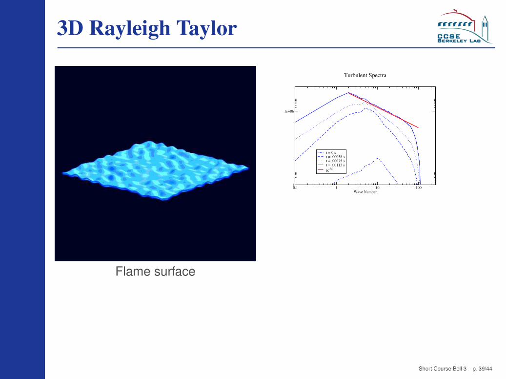
3D Rayleigh Taylor
Flame surface
0.1 1 10 100Wave Number
1
1e+06
t = 0 st = .00058 st = .00075 st = .00113 s
K-5/3
Turbulent Spectra
Short Course Bell 3 – p. 39/44
Multi-scale fluid flowsMost computations of fluid flows use a continuum representation (density,pressure, etc.) for the fluid.
Dynamics described by set of partial differential equations (PDEs).
Well-established numerical methods (finite difference, finite elements, etc.)for solving these PDEs.
The hydrodynamic PDEs are accurate over a broad range of length andtime scales.
But at some scales the continuum representation breaks down and morephysics is needed
When is the continuum description of a gas no accurate?
Knudsen number = Mean Free Path / System Length
Kn > 0.1 continuum description is not accurate
Discreteness of collisions and fluctuations are importantRarefied gasesLow-pressure manufacturingMicro-scale flows Short Course Bell 3 – p. 40/44
Hybrid methodsTo capture Knudsen effects and fluctuations we need a particle descriptionof the flow; however, these types of method are computationallyexpsensive
Can we hybridize a particle method with a continuum solver
AMR provides a framework for such a couplingAMR for fluids except change to a particle description at the finest
level of the heirarchy
Use basic AMR design paradigm for development of a hybrid methodHow to integrate a levelHow to synchronize levels
Discrete Simulation Monte Carlo (DSMC) is the dominant numericalmethod for molecular simulations of dilute gases
Short Course Bell 3 – p. 41/44
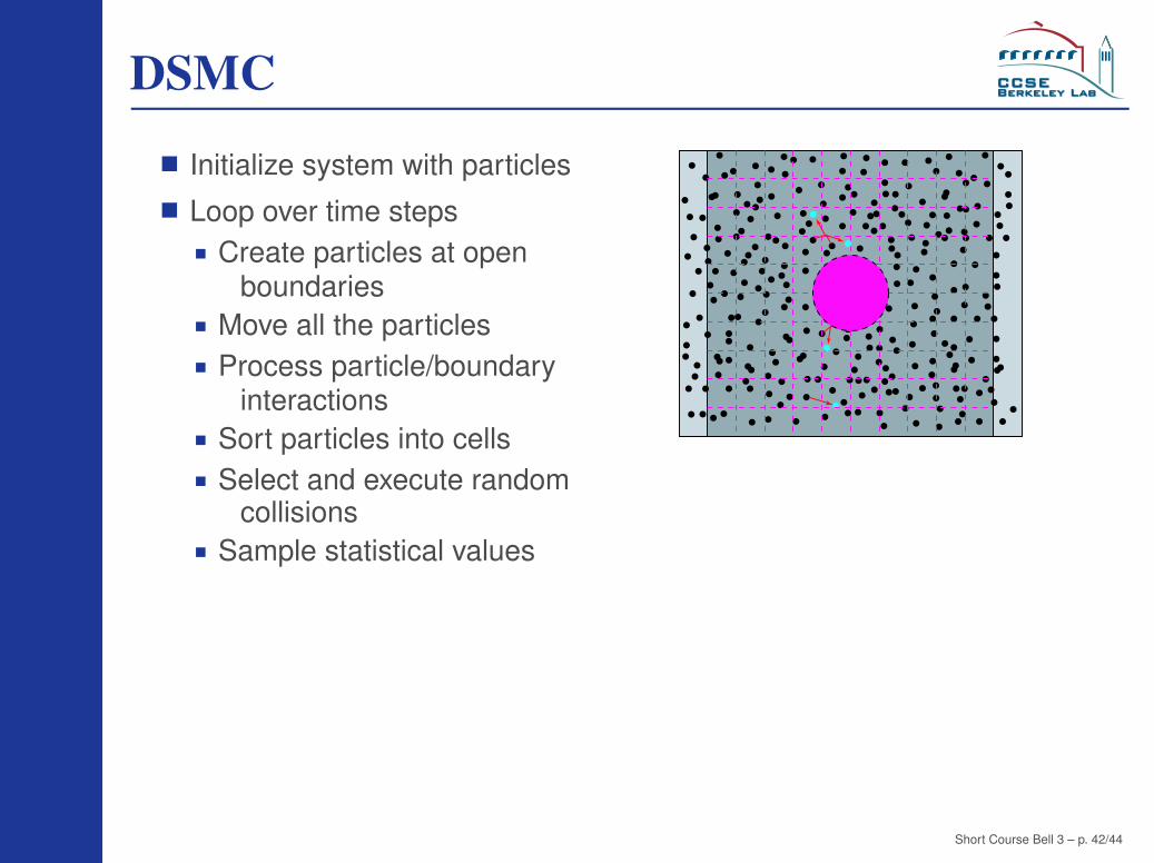
DSMC
Initialize system with particles
Loop over time stepsCreate particles at open
boundariesMove all the particlesProcess particle/boundary
interactionsSort particles into cellsSelect and execute random
collisionsSample statistical values
Short Course Bell 3 – p. 42/44

Adaptive mesh and algorithm refinement
Continuum solver – Compressible Navier Stokes
Unsplit Godunov advection
Crank-Nicolson diffusion (nonlinear multigrid)
Algorithm – 2 level
Advance continuumFT = FA + FD at DSMC boundary
Advance DMSC regionInterpolation – Sampling from
Chapman-Enskog distributionFluxes are given by particles crossing
boundary of DSMC region
SynchronizeAverage down – momentsReflux δF = −∆tAFT +
∑
p Fp
Nonlinear diffusion to distribute reflux δU
δU corrects particles to preservemoments
DSMC
Buffer cells
Continuum
DSMC boundaryconditions
A B C
D E F
1 23
DSMC flux
Short Course Bell 3 – p. 43/44
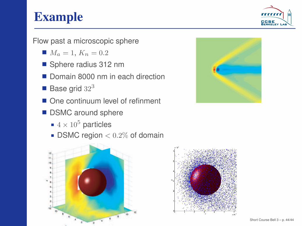
Example
Flow past a microscopic sphereMa = 1, Kn = 0.2
Sphere radius 312 nm
Domain 8000 nm in each direction
Base grid 323
One continuum level of refinmentDSMC around sphere
4 × 10⁵ particlesDSMC region < 0.2% of domain
Short Course Bell 3 – p. 44/44