Embed Size (px)
Citation preview

Block Bidiagonal Decomposition and LeastSquares Problems
Ake BjorckDepartment of Mathematics
Linkoping University
Perspectives in Numerical Analysis, Helsinki, May 27–29,2008

Outline
Bidiagonal Decomposition and LSQR
Block Bidiagonalization Methods
Multiple Right-Hand Sides in LS and TLS
Rank Deficient Blocks and Deflation
Summary

The Bidiagonal Decomposition
In 1965 Golub and Kahan gave two algorithms for computing abidiagonal decomposition (BD)
A = U(
L0
)V T ∈ Rm×n,
where B is lower bidiagonal,
B =
α1β2 α2
β3. . .. . . αn
βn+1
∈ R(n+1)×n,
and U and V are square orthogonal matrices. Givenu1 = Q1e1, the decomposition is uniquely determined ifαkβk+1 6= 0, k = 1 : n,
The Bidiagonal Decomposition
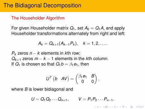
The Householder Algorithm
For given Householder matrix Q1, set A0 = Q1A, and applyHouseholder transformations alternately from right and left:
Ak = Qk+1(Ak−1Pk ), k = 1, 2, . . . .
Pk zeros n − k elements in k th row;Qk+1 zeros m − k − 1 elements in the k th column.If Q1 is chosen so that Q1b = β1e1, then
UT (b AV
)=
(β1e1 B
0 0
),
where B is lower bidiagonal and
U = Q1Q2 · · ·Qn+1, V = P1P2 · · ·Pn−1.

The Bidiagonal Decomposition
Lanczos algorithm
In the Lanczos process, successive columns of
U = (u1, u2, . . . , un+1), V = (v1, v2, . . . , vn),
with β1u1 = b, β1 = ‖b‖2, are generated recursively.Equating columns in
AT U = VBT and AV = UB,
gives the coupled two-term recurrence relations (v0 ≡ 0):
αkvk = AT uk − βkvk−1,
βk+1uk+1 = Avk − αkuk , k = 1 : n.
Here αk and βk+1 are determined by the condition‖vk‖2 = ‖uk‖2 = 1.

The Bidiagonal Decomposition
Since the BD is unique, both algorithms generate the samedecomposition in exact arithmetic.
From the Lanczos recurrences it follows that
Uk = (u1, . . . , uk ) and Vk = (v1, . . . , vk ),
form orthonormal bases for the left and rightKrylov subspaces
Kk (AAT , u1) = span[b, AAT b, . . . , (AAT )k−1b
],
Kk (AT A, v1) = span[AT b, . . . , (AT A)k−1AT b
].
If either αk = 0 or βk+1 = 0, the process terminates. Then themaximal dimensioned Krylov space has been reached.

Least Squares and LSQR
The LSQR algorithm (Paige and Saunders 1982) is a Krylovsubspace method for the LS problem
minx‖b − Ax‖2.
After k steps, one seeks an approximate solution
xk = Vkyk ∈ Kk (ATA, AT b).
From the recurrence formulas it follows that AVk = Uk+1Bk .Thus
b − AVkyk = Uk+1(β1e1 − Bkyk ),
where Bk is lower bidiagonal. By the orthogonality of Uk+1 theoptimal yk is obtained by solving a bidiagonal subproblem
miny‖β1e1 − Bky‖2,

Least Squares and LSQR
This is solved using Givens rotations to transform Bk into upperbidiagonal form
G(β1e1 | Bk ) =
(fk Rk
φk+1 0
).
givingxk = VR−1
k fk , ‖b − Axk‖2 = |φk+1|.
Then xk , k = 1, 2, 3, . . . gives approximations on a nestedsequence of Krylov subspaces. Often superior to truncatedSVD.
LSQR uses the Lanczos recursion and interleaves the solutionof the LS subproblems. A Householder implementation couldbe used for dense A.

Least Squares and LSQR
Bidiagonalization can also be used for total least squares (TLS)problems. Here the error function to be minimized is
‖b − Axk‖22
‖xk‖22 + 1
=‖β1e1 − Bkyk‖2
2
‖yk‖22 + 1
.
The solution of the lower bidiagonal TLS subproblems areobtained from the SVD of matrix(
β1e1 Bk), k = 1, 2, 3 . . . .
Partial least squares (PLS) is widely used in data analysis andstatistics. PLS is mathematically equivalent to LSQR butdifferently implemented. The predictive variables tend to bemany and are often highly correlated.

Outline
Bidiagonal Decomposition and LSQR
Block Bidiagonalization Methods
Multiple Right-Hand Sides in LS and TLS
Rank Deficient Blocks and Deflation
Summary
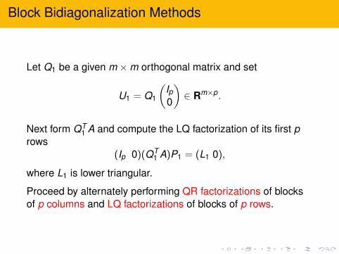
Block Bidiagonalization Methods
Let Q1 be a given m ×m orthogonal matrix and set
U1 = Q1
(Ip0
)∈ Rm×p.
Next form QT1 A and compute the LQ factorization of its first p
rows(Ip 0)(QT
1 A)P1 = (L1 0),
where L1 is lower triangular.
Proceed by alternately performing QR factorizations of blocksof p columns and LQ factorizations of blocks of p rows.

Block Bidiagonalization Methods
After k steps we have computed a block bidiagonal matrix
Tk =
L1R2 L2
. . . . . .Rk Lk
Rk+1
∈ R(k+1)p×kp,
and two block matrices with orthogonal columns
(U1, U2, . . . , Uk+1) = Qk+1 · · ·Q2Q1
(I(k+1)p
0
),
(V1, V2, . . . , Vk ) = Pk · · ·P2P1
(Ikp0
).
The matrix Tk is a banded lower triangular matrix with (p + 1)nonzero diagonals.

Block Bidiagonalization Methods
The Householder algorithm gives a constructive proof of theexistence of such a block bidiagonal decomposition.
If the LQ and QR factorizations have full rank then thedecomposition is uniquely determined by U1.
To derive a block Lanczos algorithm we use the identities
A(V1 V2 · · · Vn) = (U1 U2 · · · Un+1)Tn
AT (U1 U2 · · · Un+1) = (V1 V2 · · · Vn)T Tn .
Start by forming Z1 = AT U1 and compute its thin QRfactorization
Z1 = V1LT1 .

Block Bidiagonalization Methods
For k = 1 : n, we then do: Compute the residuals
Wk = AVk − UkLk ∈ Rm×p,
and compute the QR factorization Wk = Uk+1Rk+1.Compute the residuals
Zk+1 = AT Uk+1 − VkRTk+1 ∈ Rn×p,
and compute the QR factorization Zk+1 = Vk+1LTk+1;
Householder QR factorizations can be used to guaranteeorthogonality within each block Uk and Vk .

Block Bidiagonalization Methods
The block Lanczos bidiagonalization was given by Golub, Luk,and Overton in 1981.From the Lanczos recurrence relations it follows by inductionthat for k = 1, 2, 3, . . ., the block algorithm generatesorthogonal bases for the Krylov spaces
span(U1, . . . , Uk ) = Kk (AAT , U1),
span(V1, . . . , Vk ) = Kk (AT A, AT U1),
The process can be continued as long as the residual matriceshave full column rank. Rank deficiency will be considered later.

Outline
Bidiagonal Decomposition and LSQR
Block Bidiagonalization Methods
Multiple Right-Hand Sides in LS and TLS
Rank Deficient Blocks and Deflation
Summary

Multiple Right-Hand Sides in LS and TLS
In many applications one needs to solve least squaresproblems with multiple right-hand sides B = (b1, . . . , bp).
B = (b1, . . . , bd), d ≥ 2.
There are two possible approaches;
• Select a seed right-hand side and use the Krylov subspacegenerated to start up the solution of the second, etc.
• Use a block Krylov solver where all right-hand sides aretreated simultaneously.
Block Krylov methods:
• use a much larger search space from the start• introduce matrix–matrix multiplies into the algorithm.

Multiple Right-Hand Sides in LS and TLS
A natural generalization of LSQR is to compute a sequence ofapproximate solutions of the form
Xk = VkYk , k = 1, 2, 3, . . . ,
are determined. That is, Xk is restricted to lie in a Krylovsubspace Kk (ATA, AT B). It follows that
B − AXk = B − AVkYk = Uk+1(R1E1 − TkYk ).
Using the orthogonality of the columns of Uk+1 gives
‖B − AXk‖F = ‖R1E1 − TkYk‖F .

Block LSQR
Hence ‖B − AXk‖F is minimized for Xk ∈ R(Vk ) by takingXk = VkYk , where Yk solves
minYk
‖R1E1 − TkYk‖F .
The approximations Xk are the optimal solutions on the nestedsequence of block Krylov subspaces.
Kk (AT A, AT B), k = 1, 2, 3, . . . ..
The block bidiagonal LS subproblems are solved by usingorthogonal transformations to bring the lower triangular bandedmatrix Tk into upper triangular banded form.

Multiple Right-Hand Sides in LS and TLS
As in LSQR the solution can be interleaved with the blockbidiagonalization. For example, (p = 2)
× × × ∗ ∗∗ × ⊗ × ∗ ∗∗ ∗ ⊗ ⊗ × ∗ ∗∗ ∗ ⊗ ⊗ × ∗ ∗∗ ∗ ⊗ ⊗ × ∗∗ ∗ ⊗ × ×
× × × ×× × × ×× × × ×× × × ×
=
(C1 RX S1C2 0 S2
).
At this step the approximate solution to min ‖AX − B‖F , is
X = Vk (R−1X C1), ‖B − AX‖F = ‖C2‖f .
Residual norms are available at each step.

Multiple Right-Hand Sides in LS and TLS
The block algorithm can be used also for TLS problems withmultiple right-hand sides which is
minE , F
‖(F E
)‖F , (A + E)X = B + F ,
This cannot, as the LS problem, be reduced to p separateproblems.Using the orthogonal invariance, the error function to beminimized is
‖B − AX‖2F
‖X‖2F + 1
=‖R1E1 − TY‖2
F
‖Y‖2F + 1
.

Multiple Right-Hand Sides in LS and TLS
The TLS solution can be expressed in terms of the SVD
(B A
)=
(U1 U2
) (Σ1
Σ2
) (V T
1V T
2
),
where Σ1 = diag(σ1, . . . , σn).
The solution of the lower triangular block bidiagonal TLSproblem can be constructed from the SVD of the blockbidiagonal matrix.

Outline
Bidiagonal Decomposition and LSQR
Block Bidiagonalization Methods
Multiple Right-Hand Sides in LS and TLS
Rank Deficient Blocks and Deflation
Summary
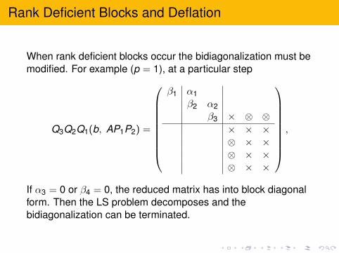
Rank Deficient Blocks and Deflation
When rank deficient blocks occur the bidiagonalization must bemodified. For example (p = 1), at a particular step
Q3Q2Q1(b, AP1P2) =
β1 α1β2 α2
β3 × ⊗ ⊗× × ×⊗ × ×⊗ × ×⊗ × ×
,
If α3 = 0 or β4 = 0, the reduced matrix has into block diagonalform. Then the LS problem decomposes and thebidiagonalization can be terminated.

Rank Deficient Blocks and Deflation
If αk = 0, then
UTk (b, AVk ) =
(β1e1 Tk 0
0 0 Ak
)and the problem is reduced to
miny‖β1e1 − Tky‖2.
Then the right Krylov vectors
AT b, (AT A)AT b, . . . , (AT A)k−1AT b
are linearly dependent.

Rank Deficient Blocks and Deflation
If βk+1 = 0, then
UTk+1(b, AVk ) =
(β1e1 Tk 0
0 0 Ak
)where Tk = (Tk αkek ) is square. Then the original system isconsistent and the solution satisfies
Tky = β1e1.
Then the left Krylov vectors
b, (AAT )b, . . . , (AAT )kb
are linearly dependent.

Rank Deficient Blocks and Deflation
From well known properties of tridiagonal matrices it follows:• The matrix Tk has full column rank and its singular values aresimple.
• The right-hand side βe1 has nonzero components along eachleft singular vector of Tk .
Paige and Strakos call this a core subproblem and shows that itis minimally dimensioned.
If we scale b := γb, then only β1 changes. Thus, we have acore subproblem for any weighted TLS problem.
min ‖(γr , E)‖F s.t. (A + E)x = b + r .

Rank Deficient Blocks and Deflation
How do we proceed in the block algorithm if a rank deficientblock occurs in an LQ or QR factorization?The triangular factor then typically has the form (p = 4 andr = rank(Rk ) = 3):
Rk =
× × × ×
0 × ×0 ×
0
∈ Rr×p.
(Recall that the factorizations are performed without pivoting).
All following elements in this diagonal of Tk will be zero.The bandwidth and block size are reduced by one.

Rank Deficient Blocks and Deflation
Example p = 2: Assume that the first element in the diagonal ofthe block R2 becomes zero.
× × ×× × ×
× × ×⊗ × ×
⊗ × ⊗⊗ × × × ×
× × × ×× × × ×× × × ×× × × ×
.
If a diagonal element (say in L3) becomes zero the problemdecomposes.
In general, the reduction can be terminated when thebandwidth has been reduced p times.

Rank Deficient Blocks and Deflation
Deflation is related to linear dependencies in the associatedKrylov subspaces:
If (AAT )kbj is linearly dependent on previous vectors, then allleft and right Krylov vectors of the form
(AAT )pbj , (AT A)pAT bj , p ≥ k ,
should be removed.
If (AT A)kAT bj is linearly dependent on previous vectors, thenall vectors of the form
(AT A)pAT bj , (AAT )p+1bj , p ≥ k ,
should be removed.
When the reduction terminates when both left and right Krylovsubspaces have reached their maximal dimensions.

Rank Deficient Blocks and Deflation
The block Lanczos algorithm is modified similarly when a rankdeficient block occurs. Recall the block Lanczos recurrence:For k = 1 : n,
VkLTk = AT Uk − Vk−1RT
k ,
Uk+1Rk+1 = AVk − UkLk .
Suppose the first rank deficient block is
Lk ∈ Rp×r , r < p.
Then Vk is n × r , i.e. only r < p vectors are determined. In thenext step
AVk − UkLk ∈ Rm×r .
Recurrence still works! Block size has been reduced to r .

Outline
Bidiagonal Decomposition and LSQR
Block Bidiagonalization Methods
Multiple Right-Hand Sides in LS and TLS
Rank Deficient Blocks and Deflation
Summary
• We have emphasized the similarity and (mathematical)equivalence of the Householder and Lanczos algorithms forblock bidiagonalization.
For dense problems in data analysis and statistics theHouseholder algorithm should be used because of its backwardstability. Today quite large dense problems can be handled inseconds on a desktop computer!
The relationship of block LSQR to multivariate PLS needsfurther investigation.
G. H. Golub and W. Kahan.Calculating the singular values and pseudo-inverse of amatrix.SIAM J. Numer. Anal. Ser. B, 2:205–224, 1965.
G. H. Golub, F. T. Luk, and M. L. Overton.A block Lanczos method for computing the singular valuesand corresponding singular vectors of a matrix.ACM Trans. Math. Software, 7:149–169, 1981.
S. Karimi and F. Toutounian.The block least squares method for solving nonsymmetriclinear systems with multiple right-hand sides.Appl. Math. Comput., 177:852–862, 2006.
C. C. Paige and M. A. Saunders.LSQR. An algorithm for sparse linear equations and sparseleast squares.ACM Trans. Math. Software, 8:43–71, 1982.