Blind Image Deblurring with Outlier Handling

Jiangxin Dong1 Jinshan Pan2 Zhixun Su1,4 Ming-Hsuan Yang3

1Dalian University of Technology 2Nanjing University of Science and Technology 3UC Merced4Guilin University of Electronic Technology

dongjxjx@gmail.com sdluran@gmail.com zxsu@dlut.edu.cn mhyang@ucmerced.edu

Abstract

Deblurring images with outliers has attracted consider-able attention recently. However, existing algorithms usual-ly involve complex operations which increase the difficultyof blur kernel estimation. In this paper, we propose a sim-ple yet effective blind image deblurring algorithm to handleblurred images with outliers. The proposed method is moti-vated by the observation that outliers in the blurred imagessignificantly affect the goodness-of-fit in function approxi-mation. Therefore, we propose an algorithm to model thedata fidelity term so that the outliers have little effect on k-ernel estimation. The proposed algorithm does not requireany heuristic outlier detection step, which is critical to thestate-of-the-art blind deblurring methods for images withoutliers. We analyze the relationship between the proposedalgorithm and other blind deblurring methods with outlierhandling and show how to estimate intermediate latent im-ages for blur kernel estimation principally. We show thatthe proposed method can be applied to generic image de-blurring as well as non-uniform deblurring. Experimentalresults demonstrate that the proposed algorithm performsfavorably against the state-of-the-art blind image deblur-ring methods on both synthetic and real-world images.

1. IntroductionSingle image deblurring has received considerable atten-

tion in recent years as more photos are taken using hand-held devices, especially with mobile smartphones. Al-though most existing smartphones are equipped with anti-shake features, inevitable camera shake results in blurredimages when taking photos in low-light conditions. Numer-ous deblurring algorithms [1, 3, 5, 10, 11, 12, 13, 14, 16,21, 23, 24, 25, 33] have been developed to address motionblur. The success of these methods can be mainly attribut-ed to the use of statistical priors from natural images (e.g.,heavy-tailed distribution of image gradients [5, 25], normal-ized sparsity prior [13], L0-regularized priors [20, 32, 33],internal patch recurrence [19], and dark channel prior [23])and salient edge selection for kernel estimation [3, 31]. Al-

though most existing methods are able to address blurredimages with a small amount of noise, these approaches arenot effective in handling blurred images with significan-t outliers, such as saturated pixels and non-Gaussian noise.

Handling blurred images with significant outliers is chal-lenging, and existing methods [4, 29] mainly address theeffects of outliers for non-blind deblurring. To addressblurred images with outliers in blind image deblurring, onetype of methods depends heavily on domain-specific prop-erties, e.g., light streaks [8, 18]. These methods are less ef-fective when the light streaks cannot be extracted and do notperform well for other types of outliers, e.g., non-Gaussiannoise. Recently, Pan et al. [22] propose an outlier handlingmethod to improve the blur kernel estimation. This methodfirst selects salient edges and then detects the regions of out-liers to refine the edge information for blur kernel estima-tion. Although this method performs well on several kindsof outliers, e.g., saturated pixels and non-Gaussian noise, itneeds complex operations and does not deblur images wellwhen the edges are not correctly selected or the regions ofoutliers cannot be detected.

It is well known that the outliers significantly affect thegoodness-of-fit in function approximation. Thus, when out-liers exist, the intermediate latent images estimated by themethods with conventional data fidelity terms [15] containsignificant artifacts and blur residues (Figure 2), which ac-cordingly affects the blur kernel estimation process. Thisis the main reason why most existing blind deblurring ap-proaches are less effective in handling blurred images withoutliers. In this paper, we propose a simple yet effectivemethod that is able to minimize the effects of outliers onthe blur kernel estimation. In contrast to existing outli-er handling algorithms [8, 18, 22], the proposed methoddoes not require complex operations, e.g., light streak de-tection [8, 18] and outlier detection [22], which are vital forexisting outlier handling methods to estimate blur kernels.

The contributions of this work are summarized as fol-lows. First, we propose a robust method to measure thegoodness-of-fit so that the effects of outliers can be min-imized in the blur kernel estimation process. Second, we

1

x*k

y

↑ Saturated pixel

x*k

y

↑ Impulse noise

(a) x and k (b) y (c) Relation of y and x ∗ k

Figure 1. Properties of saturated pixels and impulse noise. (a)Clear images x with the blur kernels k. (b) Blurred images y withsaturated pixels (top) and impulse noise (bottom). (c) Blue points:the relation between y and x ∗ k. Purple lines: the ideal case ofy = x ∗ k.present the detailed analysis on how the proposed methodperforms in the blur kernel estimation process from two per-spectives, including its mathematical essence and its weightin the iteratively re-weighted least squares (IRLS) [15] op-timization. Third, we discuss the relation between the pro-posed algorithm and other methods concerning outlier han-dling and show that the proposed method generates reliableintermediate results for blur kernel estimation without ad-hoc detection processes. Furthermore, the proposed methodperforms favorably against state-of-the-art blind deblurringmethods on both synthetic and real-world images with sig-nificant outliers. Finally, the proposed algorithm is extend-ed to handle the non-uniform deblurring effectively.

2. Proposed MethodIn this section, we develop a robust method within the

maximum a posteriori (MAP) framework to handle outliersfor blind image deblurring. We first discuss the motivationbehind the proposed method and the effects of outliers ondata fidelity terms as well as the blur kernel estimation.

2.1. MotivationA blurred image y can be modeled as a clear image x

convolved with a blur kernel k and the noise n:y = x ∗ k + n, (1)

where ∗ denotes the convolution operator. However, someintensity values of y are quite different from those of x ∗ kdue to the effect of outliers, e.g., saturated pixels and im-pulse noise (Figure 1), which cannot be well modeled bythe linear convolution model (1) and will affect both the la-tent image estimation and the blur kernel estimation.

Most deblurring methods are based on the linear convo-lution model (1), while the outliers usually have significan-t effects on the goodness-of-fit (Figure 1). Thus, existingapproaches may consider the outliers as the useful informa-tion, e.g. the salient edge, which will accordingly affect the

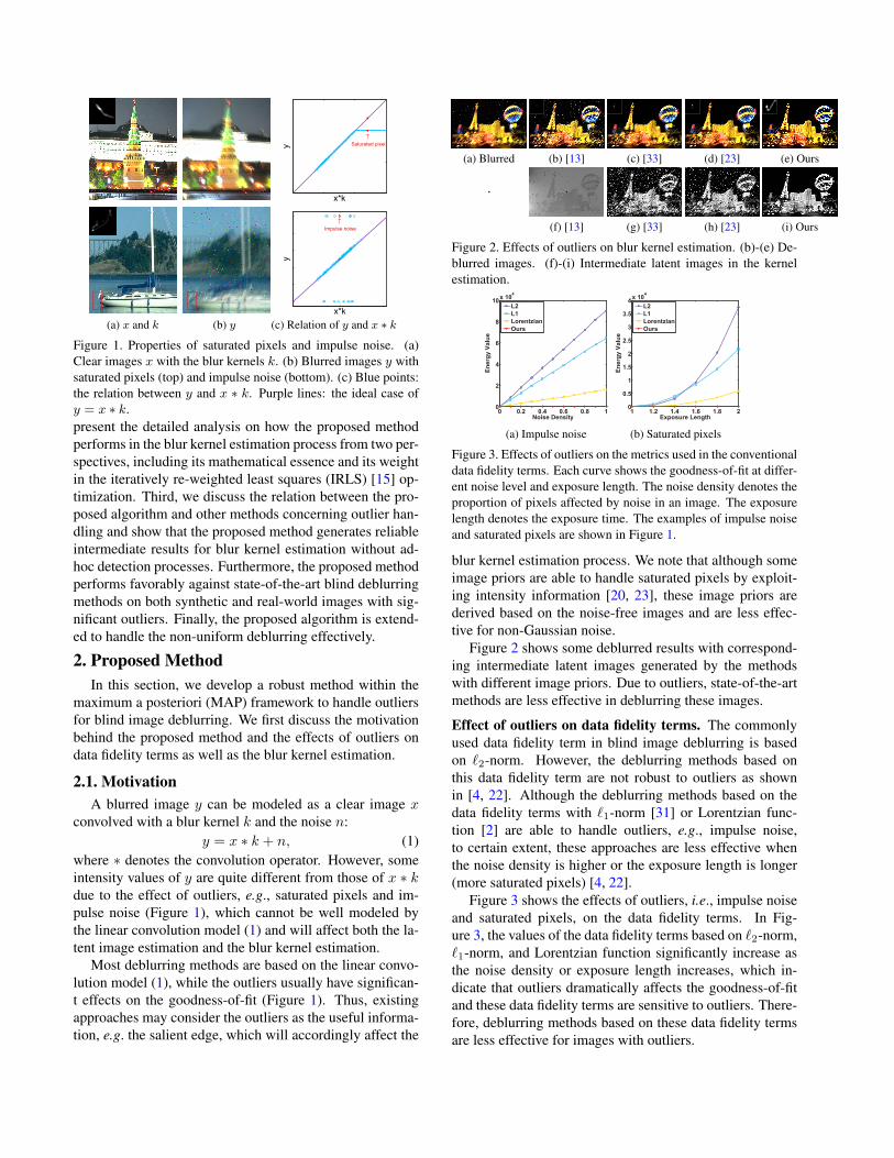
(a) Blurred (b) [13] (c) [33] (d) [23] (e) Ours

(f) [13] (g) [33] (h) [23] (i) Ours

Figure 2. Effects of outliers on blur kernel estimation. (b)-(e) De-blurred images. (f)-(i) Intermediate latent images in the kernelestimation.

0 0.2 0.4 0.6 0.8 10

2

4

6

8

10x 104

Noise Density

Ener

gy V

alue

L2L1LorentzianOurs

1 1.2 1.4 1.6 1.8 20

0.5

1

1.5

2

2.5

3

3.5

4x 104

Exposure Length

Ener

gy V

alue

L2L1LorentzianOurs

(a) Impulse noise (b) Saturated pixels

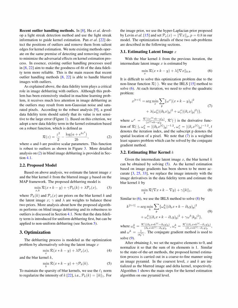
Figure 3. Effects of outliers on the metrics used in the conventionaldata fidelity terms. Each curve shows the goodness-of-fit at differ-ent noise level and exposure length. The noise density denotes theproportion of pixels affected by noise in an image. The exposurelength denotes the exposure time. The examples of impulse noiseand saturated pixels are shown in Figure 1.

blur kernel estimation process. We note that although someimage priors are able to handle saturated pixels by exploit-ing intensity information [20, 23], these image priors arederived based on the noise-free images and are less effec-tive for non-Gaussian noise.

Figure 2 shows some deblurred results with correspond-ing intermediate latent images generated by the methodswith different image priors. Due to outliers, state-of-the-artmethods are less effective in deblurring these images.

Effect of outliers on data fidelity terms. The commonlyused data fidelity term in blind image deblurring is basedon `2-norm. However, the deblurring methods based onthis data fidelity term are not robust to outliers as shownin [4, 22]. Although the deblurring methods based on thedata fidelity terms with `1-norm [31] or Lorentzian func-tion [2] are able to handle outliers, e.g., impulse noise,to certain extent, these approaches are less effective whenthe noise density is higher or the exposure length is longer(more saturated pixels) [4, 22].

Figure 3 shows the effects of outliers, i.e., impulse noiseand saturated pixels, on the data fidelity terms. In Fig-ure 3, the values of the data fidelity terms based on `2-norm,`1-norm, and Lorentzian function significantly increase asthe noise density or exposure length increases, which in-dicate that outliers dramatically affects the goodness-of-fitand these data fidelity terms are sensitive to outliers. There-fore, deblurring methods based on these data fidelity termsare less effective for images with outliers.

Recent outlier handling methods. In [8], Hu et al. devel-op a light streak detection method and use the light streakinformation to guide kernel estimation. Pan et al. [22] de-tect the positions of outliers and remove them from salientedges for kernel estimation. We note existing methods oper-ate on the same premise of detecting and removing outliersto minimize the adversarial effects on kernel estimation pro-cess. In essence, existing outlier handling processes usedin [8, 22] aim to make the goodness-of-fit of the data fideli-ty term more reliable. This is the main reason that recentoutlier handling methods [8, 22] is able to handle blurredimages with outliers.

As explained above, the data fidelity term plays a criticalrole in image deblurring with outliers. Although this prob-lem has been extensively studied in machine learning prob-lem, it receives much less attention in image deblurring asthe outliers may result from non-Gaussian noise and satu-rated pixels. According to the robust analysis [9], a gooddata fidelity term should satisfy that its value is not sensi-tive to the large error (Figure 1). Based on this criterion, weadopt a new data fidelity term in the kernel estimation basedon a robust function, which is defined as

R(z) = z2

2− log(a+ ebz

2

)

2b, (2)

where a and b are positive scalar parameters. This functionis robust to outliers as shown in Figure 3. More detailedanalysis on (2) in blind image deblurring is provided in Sec-tion 4.1.

2.2. Proposed Model

Based on above analysis, we estimate the latent image xand the blur kernel k from the blurred image y based on theMAP framework. The proposed deblurring model is

minx,kR(x ∗ k − y) + γPk(k) + λPx(x), (3)

where Pk(k) and Px(x) are priors on the blur kernel k andthe latent image x; γ and λ are weights to balance thesetwo priors. More analysis about how the proposed algorith-m performs on blind image deblurring and its robustness tooutliers is discussed in Section 4.1. Note that the data fideli-ty term is introduced for uniform deblurring first, but can beapplied to non-uniform deblurring (see Section 5).

3. OptimizationThe deblurring process is modeled as the optimization

problem by alternatively solving the latent image x

minxR(x ∗ k − y) + λPx(x), (4)

and the blur kernel k,

minkR(x ∗ k − y) + γPk(k). (5)

To maintain the sparsity of blur kernels, we use the `1 normto regularize the intensity of k [22], i.e., Pk(k) = ‖k‖1. For

the image prior, we use the hyper-Laplacian prior proposedby Levin et al. [15] and set Px(x) = ‖∇x‖p, p = 0.8 in ourmodel. The optimization details of these two sub-problemsare described in the following sections.

3.1. Estimating Latent Image x

With the blur kernel k from the previous iteration, theintermediate latent image x is estimated by

minxR(x ∗ k − y) + λ‖∇x‖0.8. (6)

It is difficult to solve this optimization problem due to thenon-linear function R(·). We use the IRLS [15] method tosolve (6). At each iteration, we need to solve the quadraticproblem:

x[t+1] =argminx

∑p

{ωx|(x ∗ k − y)p|2

+ λ(ωxh|(∂hx)p|2 + ωx

v |(∂vx)p|2)},(7)

where ωx =R′((x[t]∗k−y)p)

(x[t]∗k−y)p, R′(·) is the derivative func-

tion of R(·), ωxh = |(∂hx[t])p|−1.2, ωx

v = |(∂vx[t])p|−1.2, tdenotes the iteration index, and the subscript p denotes thespatial location of a pixel. We note that (7) is a weightedleast squares problem which can be solved by the conjugategradient method.

3.2. Estimating Blur Kernel k

Given the intermediate latent image x, the blur kernel kcan be obtained by solving (5). As the kernel estimationbased on image gradients has been shown to be more ac-curate [3, 25, 33], we replace the image intensity with theimage derivatives in the data fidelity term and estimate theblur kernel k by

minkR(∇x ∗ k −∇y) + γ‖k‖1. (8)

Similar to (6), we use the IRLS method to solve (8) by

k[t+1] =argmink

∑p

{ωkh|(∂hx ∗ k − ∂hy)p|2

+ ωkv |(∂vx ∗ k − ∂vy)p|2 + γωk|kp|2},

(9)

where ωkh =

R′((∂hx∗k[t]−∂hy)p)

(∂hx∗k[t]−∂hy)p, ωk

v =R′((∂vx∗k[t]−∂vy)p)

(∂vx∗k[t]−∂vy)p,

and ωk = 1

|k[t]p |

. The conjugate gradient method is used to

solve (9).After obtaining k, we set the negative elements to 0, and

normalize it so that the sum of its elements is 1. Similarto the state-of-the-art methods, the proposed kernel estima-tion process is carried out in a coarse-to-fine manner usingan image pyramid. In the coarsest level, x and k are ini-tialized as the blurred image and delta kernel, respectively.Algorithm 1 shows the main steps for the kernel estimationalgorithm on one pyramid level.

Algorithm 1 Blur kernel estimation algorithmInput: Blurred image y.initial k with results from the coarser level.for i ≤ tmax do

Estimate x according to (7).Estimate k according to (9).

end forOutput: Blur kernel k and latent image x.

−0.5 0 0.50

1

2x 10−3

−0.1 −0.05 0 0.05 0.10

0.2

0.4

0.6

0.8

1

(a)R(z) (b) R′(z)z

Figure 4. Visualization of the robust functionR(z) and the weight,i.e., R′(z)

z, used in IRLS.

4. Analysis of Proposed MethodIn this section, we analyze how the proposed algorithm

performs on blind image deblurring with outliers. We alsodemonstrate the effectiveness of the proposed data fideli-ty term for blur kernel estimation with outlier handling. Inaddition, we discuss the relationship of the proposed algo-rithm with other methods in terms of handling outliers.

4.1. Effectivness of Proposed Method

As discussed in Section 2.1, the proposed data fidelityterm is robust to outliers. From the definition of the robustfunction (2), the Taylor polynomial approximation of R(z)with respect to z at 0 is

R(z) = a

2a+ 2z2 − log(a+ 1)

2b+O(z3), (10)

where O(·) denotes the equivalent infinitesimal. The Tay-lor expansion of R(z) means that R(z) has the same orderwith z2 if the value of z is close to zero. This propertydemonstrates that the proposed intermediate latent imageestimation model (4) will reduce to the sparse deconvolu-tion model by Levin et al. [16], which is effective for theimage deconvolution without outliers. Figure 4 shows thatR(z) is close to a constant when the value of z is large1. Inthis case, the model (4) reduces to a constant plus the reg-ularization term. Thus, only the regularization term has aneffect on the image restoration, which indicates that mostoutliers will be smoothed. This property ensures that thedeblurring method based on (2) is able to handle outliers.

From the perspective of the IRLS iteration, the weightfor the data fidelity term is R

′(z)z . It has a small value when

1The value of (x ∗ k− y) at pixel p is large if pixel p is an outlier, andis small otherwise (Figure 1).

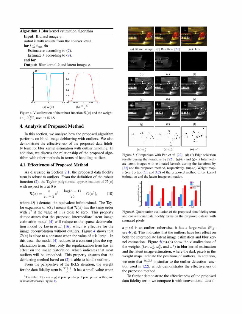
(a) Blurred image (b) Results of [22] (c) Ours

(d) (e) (f)

(g) (h) (i)

(j) (k) (l)

(m) ωkh (n) ωk

v (o) ωx

Figure 5. Comparison with Pan et al. [22]. (d)-(f) Edge selectionresults during the iterations by [22]. (g)-(i) and (j)-(l) Intermedi-ate latent images with estimated kernels during the iterations by[22] and the proposed method, respectively. (m)-(o) Weight map-s (see Section 3.1 and 3.2) of the proposed method in the kernelestimation and the latent image estimation.

im1 im2 im3 im4 im526

28

30

32

34

36

Aver

age

PSN

R V

alue

s

L2L1LorentzianOurs

Figure 6. Quantitative evaluation of the proposed data fidelity termand conventional data fidelity terms on the proposed dataset withsaturated pixels.

a pixel is an outlier; otherwise, it has a large value (Fig-ure 4(b)). This indicates that the outliers have less effect onboth the intermediate latent image estimation and blur ker-nel estimation. Figure 5(m)-(o) show the visualizations ofthe weights (i.e., ωk

h, ωkv , and ωx) in blur kernel estimation

and the latent image estimation, where the dark pixels in theweight maps indicate the positions of outliers. In addition,we note that R

′(z)z is similar to the outlier detection func-

tion used in [22], which demonstrates the effectiveness ofthe proposed method.

To further demonstrate the effectiveness of the proposeddata fidelity term, we compare it with conventional data fi-

(a) Blurred (b) L2 (c) L1 (d) Lorentzian (e) Ours

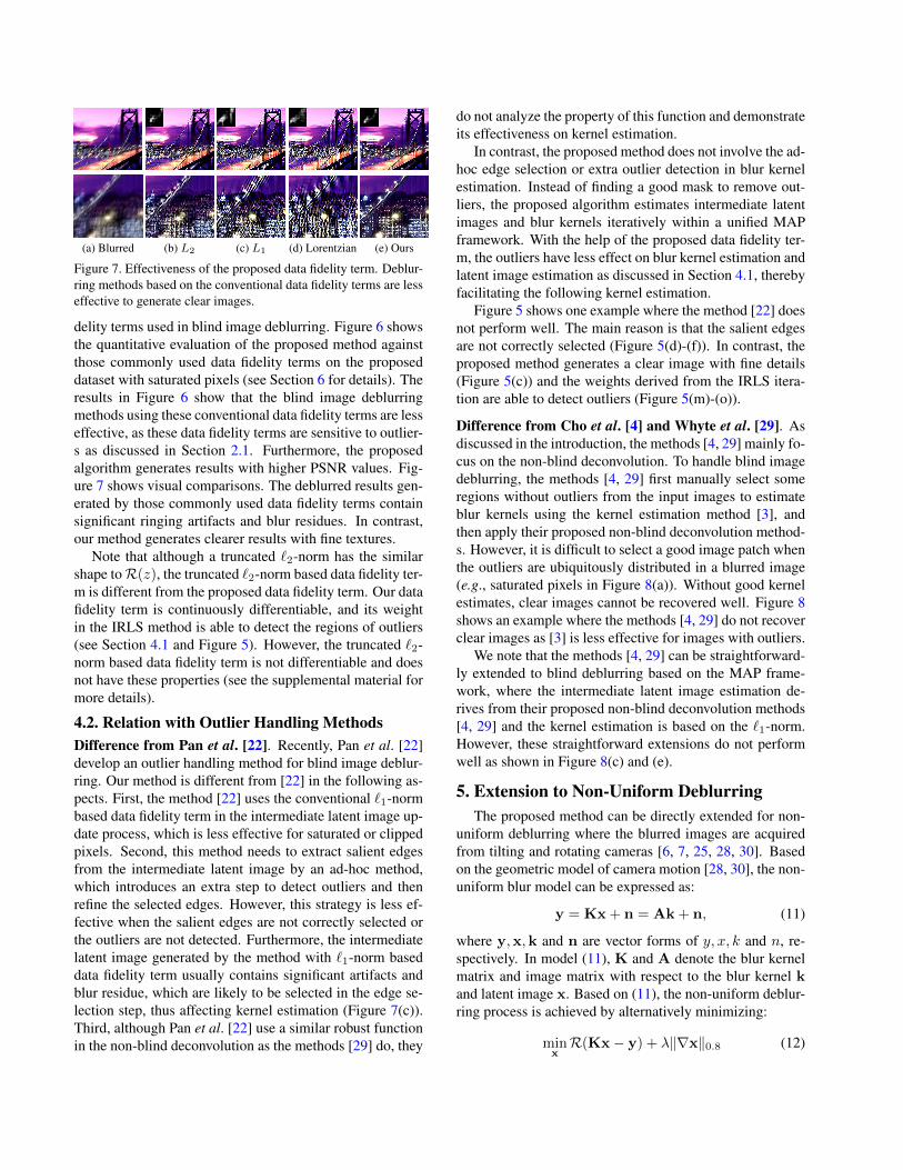
Figure 7. Effectiveness of the proposed data fidelity term. Deblur-ring methods based on the conventional data fidelity terms are lesseffective to generate clear images.

delity terms used in blind image deblurring. Figure 6 showsthe quantitative evaluation of the proposed method againstthose commonly used data fidelity terms on the proposeddataset with saturated pixels (see Section 6 for details). Theresults in Figure 6 show that the blind image deblurringmethods using these conventional data fidelity terms are lesseffective, as these data fidelity terms are sensitive to outlier-s as discussed in Section 2.1. Furthermore, the proposedalgorithm generates results with higher PSNR values. Fig-ure 7 shows visual comparisons. The deblurred results gen-erated by those commonly used data fidelity terms containsignificant ringing artifacts and blur residues. In contrast,our method generates clearer results with fine textures.

Note that although a truncated `2-norm has the similarshape toR(z), the truncated `2-norm based data fidelity ter-m is different from the proposed data fidelity term. Our datafidelity term is continuously differentiable, and its weightin the IRLS method is able to detect the regions of outliers(see Section 4.1 and Figure 5). However, the truncated `2-norm based data fidelity term is not differentiable and doesnot have these properties (see the supplemental material formore details).

4.2. Relation with Outlier Handling MethodsDifference from Pan et al. [22]. Recently, Pan et al. [22]develop an outlier handling method for blind image deblur-ring. Our method is different from [22] in the following as-pects. First, the method [22] uses the conventional `1-normbased data fidelity term in the intermediate latent image up-date process, which is less effective for saturated or clippedpixels. Second, this method needs to extract salient edgesfrom the intermediate latent image by an ad-hoc method,which introduces an extra step to detect outliers and thenrefine the selected edges. However, this strategy is less ef-fective when the salient edges are not correctly selected orthe outliers are not detected. Furthermore, the intermediatelatent image generated by the method with `1-norm baseddata fidelity term usually contains significant artifacts andblur residue, which are likely to be selected in the edge se-lection step, thus affecting kernel estimation (Figure 7(c)).Third, although Pan et al. [22] use a similar robust functionin the non-blind deconvolution as the methods [29] do, they

do not analyze the property of this function and demonstrateits effectiveness on kernel estimation.

In contrast, the proposed method does not involve the ad-hoc edge selection or extra outlier detection in blur kernelestimation. Instead of finding a good mask to remove out-liers, the proposed algorithm estimates intermediate latentimages and blur kernels iteratively within a unified MAPframework. With the help of the proposed data fidelity ter-m, the outliers have less effect on blur kernel estimation andlatent image estimation as discussed in Section 4.1, therebyfacilitating the following kernel estimation.

Figure 5 shows one example where the method [22] doesnot perform well. The main reason is that the salient edgesare not correctly selected (Figure 5(d)-(f)). In contrast, theproposed method generates a clear image with fine details(Figure 5(c)) and the weights derived from the IRLS itera-tion are able to detect outliers (Figure 5(m)-(o)).

Difference from Cho et al. [4] and Whyte et al. [29]. Asdiscussed in the introduction, the methods [4, 29] mainly fo-cus on the non-blind deconvolution. To handle blind imagedeblurring, the methods [4, 29] first manually select someregions without outliers from the input images to estimateblur kernels using the kernel estimation method [3], andthen apply their proposed non-blind deconvolution method-s. However, it is difficult to select a good image patch whenthe outliers are ubiquitously distributed in a blurred image(e.g., saturated pixels in Figure 8(a)). Without good kernelestimates, clear images cannot be recovered well. Figure 8shows an example where the methods [4, 29] do not recoverclear images as [3] is less effective for images with outliers.

We note that the methods [4, 29] can be straightforward-ly extended to blind deblurring based on the MAP frame-work, where the intermediate latent image estimation de-rives from their proposed non-blind deconvolution methods[4, 29] and the kernel estimation is based on the `1-norm.However, these straightforward extensions do not performwell as shown in Figure 8(c) and (e).

5. Extension to Non-Uniform DeblurringThe proposed method can be directly extended for non-

uniform deblurring where the blurred images are acquiredfrom tilting and rotating cameras [6, 7, 25, 28, 30]. Basedon the geometric model of camera motion [28, 30], the non-uniform blur model can be expressed as:

y = Kx+ n = Ak+ n, (11)

where y,x,k and n are vector forms of y, x, k and n, re-spectively. In model (11), K and A denote the blur kernelmatrix and image matrix with respect to the blur kernel kand latent image x. Based on (11), the non-uniform deblur-ring process is achieved by alternatively minimizing:

minxR(Kx− y) + λ‖∇x‖0.8 (12)

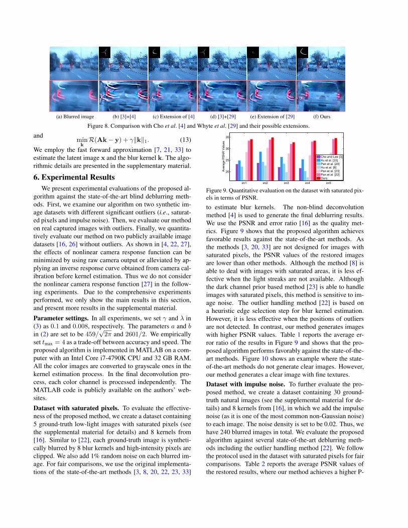
(a) Blurred image (b) [3]+[4] (c) Extension of [4] (d) [3]+[29] (e) Extension of [29] (f) Ours

Figure 8. Comparison with Cho et al. [4] and Whyte et al. [29] and their possible extensions.

andminkR(Ak− y) + γ‖k‖1. (13)

We employ the fast forward approximation [7, 21, 33] toestimate the latent image x and the blur kernel k. The algo-rithmic details are presented in the supplementary material.

6. Experimental ResultsWe present experimental evaluations of the proposed al-

gorithm against the state-of-the-art blind deblurring meth-ods. First, we examine our algorithm on two synthetic im-age datasets with different significant outliers (i.e., saturat-ed pixels and impulse noise). Then, we evaluate our methodon real captured images with outliers. Finally, we quantita-tively evaluate our method on two publicly available imagedatasets [16, 26] without outliers. As shown in [4, 22, 27],the effects of nonlinear camera response function can beminimized by using raw camera output or alleviated by ap-plying an inverse response curve obtained from camera cal-ibration before kernel estimation. Thus we do not considerthe nonlinear camera response function [27] in the follow-ing experiments. Due to the comprehensive experimentsperformed, we only show the main results in this section,and present more results in the supplemental material.

Parameter settings. In all experiments, we set γ and λ in(3) as 0.1 and 0.008, respectively. The parameters a and bin (2) are set to be 459/

√2π and 2601/2. We empirically

set tmax = 4 as a trade-off between accuracy and speed. Theproposed algorithm is implemented in MATLAB on a com-puter with an Intel Core i7-4790K CPU and 32 GB RAM.All the color images are converted to grayscale ones in thekernel estimation process. In the final deconvolution pro-cess, each color channel is processed independently. TheMATLAB code is publicly available on the authors’ web-sites.

Dataset with saturated pixels. To evaluate the effective-ness of the proposed method, we create a dataset containing5 ground-truth low-light images with saturated pixels (seethe supplemental material for details) and 8 kernels from[16]. Similar to [22], each ground-truth image is syntheti-cally blurred by 8 blur kernels and high-intensity pixels areclipped. We also add 1% random noise on each blurred im-age. For fair comparisons, we use the original implementa-tions of the state-of-the-art methods [3, 8, 20, 22, 23, 33]

im1 im2 im3 im4 im5

20

25

30

35

Aver

age

PSN

R V

alue

s

Cho and Lee [3]Xu et al. [33]Pan et al. [20]Hu et al. [8]Pan et al. [23]Pan et al. [22]Ours

Figure 9. Quantitative evaluation on the dataset with saturated pix-els in terms of PSNR.

to estimate blur kernels. The non-blind deconvolutionmethod [4] is used to generate the final deblurring results.We use the PSNR and error ratio [16] as the quality met-rics. Figure 9 shows that the proposed algorithm achievesfavorable results against the state-of-the-art methods. Asthe methods [3, 20, 33] are not designed for images withsaturated pixels, the PSNR values of the restored imagesare lower than other methods. Although the method [8] isable to deal with images with saturated areas, it is less ef-fective when the light streaks are not available. Althoughthe dark channel prior based method [23] is able to handleimages with saturated pixels, this method is sensitive to im-age noise. The outlier handling method [22] is based ona heuristic edge selection step for blur kernel estimation.However, it is less effective when the positions of outliersare not detected. In contrast, our method generates imageswith higher PSNR values. Table 1 reports the average er-ror ratio of the results in Figure 9 and shows that the pro-posed algorithm performs favorably against the state-of-the-art methods. Figure 10 shows an example where the state-of-the-art methods do not generate clear images. However,our method generates a clear image with fine textures.Dataset with impulse noise. To further evaluate the pro-posed method, we create a dataset containing 30 ground-truth natural images (see the supplemental material for de-tails) and 8 kernels from [16], in which we add the impulsenoise (as it is one of the most common non-Gaussian noise)to each image. The noise density is set to be 0.02. Thus, wehave 240 blurred images in total. We evaluate the proposedalgorithm against several state-of-the-art deblurring meth-ods including the outlier handling method [22]. We followthe protocol used in the dataset with saturated pixels for faircomparisons. Table 2 reports the average PSNR values ofthe restored results, where our method achieves a higher P-

Table 1. Quantitative comparison using the dataset with saturated pixels in terms of error ratio metric.[3] [33] [20] [8] [23] [22] Ours

Average Error Ratio 18.04 7.42 13.41 34.37 3.83 3.22 3.09

(a) Input (b) [3] (c) [33] (d) [8]PSNR: 14.72 PSNR: 21.60 PSNR: 17.89 PSNR: 20.11

(e) [23] (f) [22] (g) Ours (h) GTPSNR: 19.33 PSNR: 21.11 PSNR: 23.52

Figure 10. A synthetic example with saturated pixels (Best viewedon high-resolution displays with zoom-in).

2 4 6 8 10 12 14 16 18 200

10

20

30

40

50

60

70

80

90

100

110

Error Ratios

Succ

ess

Rat

e (%

)

OursPan et al. [22]Pan et al. [23]Zhong et al. [34]Xu et al. [33]Levin et al. [17]Cho and Lee [3]

0.01 0.02 0.03 0.04 0.0524

26

28

30

32

34

36

Noise Density (%)

Ave

rage

PSN

R V

alue

s

OursPan et al. [22]Pan et al. [23]Zhong et al. [34]Xu et al. [33]

(a) Dataset with impulse noise (b) Robustness to impulse noise

Figure 11. Quantitative evaluations on dataset with impulse noise.

SNR than the others. The error ratio [16] is also used asthe quality metric. As Figure 11(a) shows, our method per-forms favorably against the state-of-the-art methods.

We evaluate our method using images with differen-t noise densities. Figure 11(b) shows that the proposed al-gorithm performs well even when the noise density is high.

Figure 12 shows a synthetic example with impulse noisefrom the dataset. Since the conventional data fidelity termsare not robust to outliers, the state-of-the-art blind deblur-ring algorithms [3, 17, 33] do not estimate the blur kernelswell, thus resulting in blurred results with significant ring-ing artifacts (Figure 12(b), (c), and (d)). The method [34] isdesigned to deal with Gaussian noise, but less effective forimpulse noise. Although the recent method [23] is able toaddress saturated images, it is less effective for images withnoise as pointed in the work. Thus, the blur kernels esti-mated by [23, 34] are not accurate which accordingly lead-s to results with significant ringing artifacts (Figure 12(e)and (f)). The method [22] is designed to handle outlier-s including impulse noise. However, this method involvesa heuristic edge selection and outlier detection step and isless effective when the edges are not correctly selected orthe outliers are not detected (Figure 12(g)). In contrast, ourestimated blur kernel is visually close to the ground-truthblur kernel, and the recovered latent image contains clearerdetails and fewer ringing artifacts (Figure 12(h)).

Real images. We evaluate the proposed algorithm and oth-er methods using real images with outliers. Figures 13

(a) Input (b) [3] (c) [17] (d) [33]PSNR: 16.00 PSNR: 20.05 PSNR: 26.13 PSNR: 26.12

(e) [34] (f) [22] (g) Ours (h) GTPSNR: 22.31 PSNR: 28.76 PSNR: 31.37

Figure 12. A synthetic example with impulse noise (Best viewedon high-resolution displays with zoom-in).

(a) Blurred (b) [3] (c) [17] (d) [33]

(e) [8] (f) [23] (g) [22] (h) Ours

Figure 13. A real captured image with numerous saturated pixels.

and 14 show two challenging real captured images withnumerous saturated areas and unknown noise. The state-of-the-art methods [3, 17, 23, 33] do not perform well onthese examples due to the effects of saturated areas. Themethod by Hu et al. [8] does not generate clear resultseither due to unavailable light streaks (Figures 13(e) and14(e)). The deblurred results of [22] contain ringing arti-facts, and some details are not recovered well. In contrast,our method successfully estimates the blur kernels and gen-erates better-deblurred results. Furthermore, the compari-son results shown in Figures 13 and 14 demonstrate that theproposed algorithm is able to prevent the effects of outliersin blur kernel estimation.

Non-uniform examples. As our method can be extended to

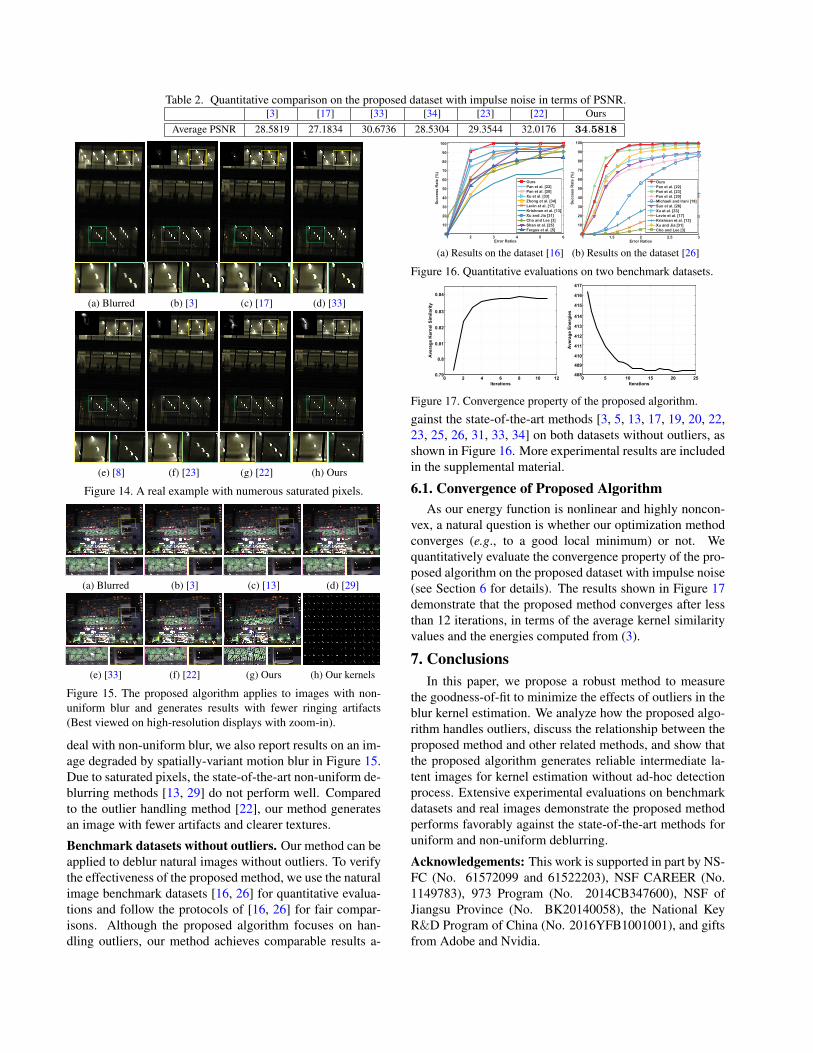
Table 2. Quantitative comparison on the proposed dataset with impulse noise in terms of PSNR.[3] [17] [33] [34] [23] [22] Ours

Average PSNR 28.5819 27.1834 30.6736 28.5304 29.3544 32.0176 34.5818

(a) Blurred (b) [3] (c) [17] (d) [33]

(e) [8] (f) [23] (g) [22] (h) Ours

Figure 14. A real example with numerous saturated pixels.

(a) Blurred (b) [3] (c) [13] (d) [29]

(e) [33] (f) [22] (g) Ours (h) Our kernels

Figure 15. The proposed algorithm applies to images with non-uniform blur and generates results with fewer ringing artifacts(Best viewed on high-resolution displays with zoom-in).

deal with non-uniform blur, we also report results on an im-age degraded by spatially-variant motion blur in Figure 15.Due to saturated pixels, the state-of-the-art non-uniform de-blurring methods [13, 29] do not perform well. Comparedto the outlier handling method [22], our method generatesan image with fewer artifacts and clearer textures.

Benchmark datasets without outliers. Our method can beapplied to deblur natural images without outliers. To verifythe effectiveness of the proposed method, we use the naturalimage benchmark datasets [16, 26] for quantitative evalua-tions and follow the protocols of [16, 26] for fair compar-isons. Although the proposed algorithm focuses on han-dling outliers, our method achieves comparable results a-

1 2 3 4 5 60

10

20

30

40

50

60

70

80

90

100

Error Ratios

Succ

ess

Rat

e (%

)

OursPan et al. [22]Pan et al. [20]Xu et al. [33]Zhong et al. [34]Levin et al. [17]Krishnan et al. [13]Xu and Jia [31]Cho and Lee [3]Shan et al. [25]Fergus et al. [5]

1 1.5 2 2.5 30

10

20

30

40

50

60

70

80

90

100

Error Ratios

Succ

ess

Rat

e (%

)

OursPan et al. [22]Pan et al. [23]Pan et al. [20]Michaeli and Irani [19]Sun et al. [26]Xu et al. [33]Levin et al. [17]Krishnan et al. [13]Xu and Jia [31]Cho and Lee [3]

(a) Results on the dataset [16] (b) Results on the dataset [26]

Figure 16. Quantitative evaluations on two benchmark datasets.

0 2 4 6 8 10 120.79

0.8

0.81

0.82

0.83

0.84

Iterations

Ave

rage

Ker

nel S

imila

rity

0 5 10 15 20 25408

409

410

411

412

413

414

415

416

417

Iterations

Ave

rage

Ene

rgie

s

Figure 17. Convergence property of the proposed algorithm.

gainst the state-of-the-art methods [3, 5, 13, 17, 19, 20, 22,23, 25, 26, 31, 33, 34] on both datasets without outliers, asshown in Figure 16. More experimental results are includedin the supplemental material.

6.1. Convergence of Proposed AlgorithmAs our energy function is nonlinear and highly noncon-

vex, a natural question is whether our optimization methodconverges (e.g., to a good local minimum) or not. Wequantitatively evaluate the convergence property of the pro-posed algorithm on the proposed dataset with impulse noise(see Section 6 for details). The results shown in Figure 17demonstrate that the proposed method converges after lessthan 12 iterations, in terms of the average kernel similarityvalues and the energies computed from (3).

7. ConclusionsIn this paper, we propose a robust method to measure

the goodness-of-fit to minimize the effects of outliers in theblur kernel estimation. We analyze how the proposed algo-rithm handles outliers, discuss the relationship between theproposed method and other related methods, and show thatthe proposed algorithm generates reliable intermediate la-tent images for kernel estimation without ad-hoc detectionprocess. Extensive experimental evaluations on benchmarkdatasets and real images demonstrate the proposed methodperforms favorably against the state-of-the-art methods foruniform and non-uniform deblurring.

Acknowledgements: This work is supported in part by NS-FC (No. 61572099 and 61522203), NSF CAREER (No.1149783), 973 Program (No. 2014CB347600), NSF ofJiangsu Province (No. BK20140058), the National KeyR&D Program of China (No. 2016YFB1001001), and giftsfrom Adobe and Nvidia.

References[1] J.-F. Cai, H. Ji, C. Liu, and Z. Shen. Blind motion deblurring

from a single image using sparse approximation. In CVPR,pages 104–111, 2009.

[2] J. Chen, L. Yuan, C. Tang, and L. Quan. Robust dual motiondeblurring. In CVPR, 2008.

[3] S. Cho and S. Lee. Fast motion deblurring. ACM TOG,28(5):145, 2009.

[4] S. Cho, J. Wang, and S. Lee. Handling outliers in non-blindimage deconvolution. In ICCV, pages 495–502, 2011.

[5] R. Fergus, B. Singh, A. Hertzmann, S. T. Roweis, and W. T.Freeman. Removing camera shake from a single photograph.ACM TOG, 25(3):787–794, 2006.

[6] A. Gupta, N. Joshi, C. L. Zitnick, M. Cohen, and B. Curless.Single image deblurring using motion density functions. InECCV, pages 171–184, 2010.

[7] M. Hirsch, C. J. Schuler, S. Harmeling, and B. Scholkopf.Fast removal of non-uniform camera shake. In ICCV, pages463–470, 2011.

[8] Z. Hu, S. Cho, J. Wang, and M. H. Yang. Deblurring low-light images with light streaks. In CVPR, pages 3382–3389,2014.

[9] P. J. Huber. Robust Statistics. Springer, 1981.[10] J. Jia. Mathematical models and practical solvers for unifor-

m motion deblurring. Cambridge University Press, 2014.[11] N. Joshi, R. Szeliski, and D. J. Kriegman. PSF estimation

using sharp edge prediction. In CVPR, pages 1–8, 2008.[12] R. Kohler, M. Hirsch, B. Mohler, B. Scholkopf, and

S. Harmeling. Recording and playback of camerashake: Benchmarking blind deconvolution with a real-worlddatabase. In ECCV, pages 27–40, 2012.

[13] D. Krishnan, T. Tay, and R. Fergus. Blind deconvolutionusing a normalized sparsity measure. In CVPR, pages 2657–2664, 2011.

[14] S. Lee and S. Cho. Recent advances in image deblurring. InSIGGRAPH Asia 2013 Courses, 2013.

[15] A. Levin, R. Fergus, F. Durand, and W. T. Freeman. Imageand depth from a conventional camera with a coded aperture.ACM TOG, 26(3):70, 2007.

[16] A. Levin, Y. Weiss, F. Durand, and W. T. Freeman. Under-standing and evaluating blind deconvolution algorithms. InCVPR, pages 1964–1971, 2009.

[17] A. Levin, Y. Weiss, F. Durand, and W. T. Freeman. Efficientmarginal likelihood optimization in blind deconvolution. InCVPR, pages 2657–2664, 2011.

[18] H. Liu, X. Sun, L. Fang, and F. Wu. Deblurring satu-rated night image with function-form kernel. IEEE TIP,24(11):4637–4650, 2015.

[19] T. Michaeli and M. Irani. Blind deblurring using internalpatch recurrence. In ECCV, pages 783–798, 2014.

[20] J. Pan, Z. Hu, Z. Su, and M.-H. Yang. Deblurring text imagesvia L0-regularized intensity and gradient prior. In CVPR,pages 2901–2908, 2014.

[21] J. Pan, Z. Hu, Z. Su, and M.-H. Yang. L0-regularized intensi-ty and gradient prior for deblurring text images and beyond.IEEE TPAMI, 39(2):342–355, 2017.

[22] J. Pan, Z. Lin, Z. Su, and M.-H. Yang. Robust kernel estima-tion with outliers handling for image deblurring. In CVPR,pages 2800–2808, 2016.

[23] J. Pan, D. Sun, H. Pfister, and M.-H. Yang. Blind imagedeblurring using dark channel prior. In CVPR, pages 1628–1636, 2016.

[24] D. Perrone and P. Favaro. Total variation blind deconvolu-tion: The devil is in the details. In CVPR, pages 2909–2916,2014.

[25] Q. Shan, J. Jia, and A. Agarwala. High-quality motion de-blurring from a single image. ACM TOG, 27(3):73, 2008.

[26] L. Sun, S. Cho, J. Wang, and J. Hays. Edge-based blur kernelestimation using patch priors. In ICCP, 2013.

[27] Y.-W. Tai, X. Chen, S. Kim, S. J. Kim, F. Li, J. Yang, J. Yu,Y. Matsushita, and M. S. Brown. Nonlinear camera responsefunctions and image deblurring: Theoretical analysis andpractice. IEEE TPAMI, 35(10):2498–2512, 2013.

[28] Y.-W. Tai, P. Tan, and M. S. Brown. Richardson-lucy deblur-ring for scenes under a projective motion path. IEEE TPAMI,33(8):1603–1618, 2011.

[29] O. Whyte, J. Sivic, and A. Zisserman. Deblurring shakenand partially saturated images. IJCV, 110(2):185–201, 2014.

[30] O. Whyte, J. Sivic, A. Zisserman, and J. Ponce. Non-uniformdeblurring for shaken images. IJCV, 98(2):168–186, 2012.

[31] L. Xu and J. Jia. Two-phase kernel estimation for robustmotion deblurring. In ECCV, pages 157–170, 2010.

[32] L. Xu, C. Lu, Y. Xu, and J. Jia. Image smoothing via L0

gradient minimization. ACM TOG, 30(6):174, 2011.[33] L. Xu, S. Zheng, and J. Jia. Unnatural L0 sparse represen-

tation for natural image deblurring. In CVPR, pages 1107–1114, 2013.

[34] L. Zhong, S. Cho, D. Metaxas, S. Paris, and J. Wang. Han-dling noise in single image deblurring using directional fil-ters. In CVPR, pages 612–619, 2013.