Embed Size (px)
Citation preview

I,' II1k. 0
C 0-1
Blair Fyffe
A thesis submitted for the degree of Doctor of Philosophy. The University ofr Edinburgh.
December 2006
Abstract
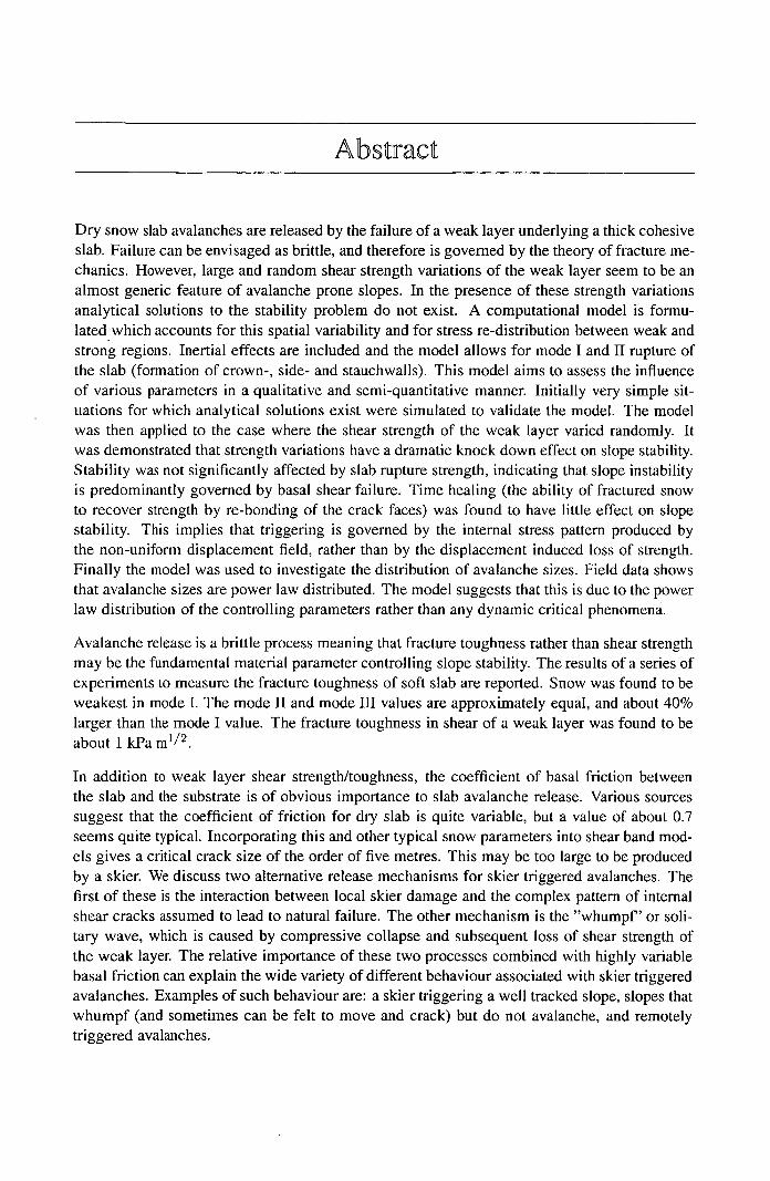
Dry snow slab avalanches are released by the failure of a weak layer underlying a thick cohesive slab. Failure can be envisaged as brittle, and therefore is governed by the theory of fracture me-chanics. However, large and random shear strength variations of the weak layer seem to be an almost generic feature of avalanche prone slopes. In the presence of these strength variations analytical solutions to the stability problem do not exist. A computational model is formu-lated which accounts for this spatial variability and for stress re-distribution between weak and strong regions. Inertial effects are included and the model allows for mode I and II rupture of the slab (formation of crown-, side- and stauchwalls). This model aims to assess the influence of various parameters in a qualitative and semi-quantitative manner. Initially very simple sit-uations for which analytical solutions exist were simulated to validate the model. The model was then applied to the case where the shear strength of the weak layer varied randomly. It was demonstrated that strength variations have a dramatic knock down effect on slope stability. Stability was not significantly affected by slab rupture strength, indicating that slope instability is predominantly governed by basal shear failure. Time healing (the ability of fractured snow to recover strength by re-bonding of the crack faces) was found to have little effect on slope stability. This implies that triggering is governed by the internal stress pattern produced by the non-uniform displacement field, rather than by the displacement induced loss of strength. Finally the model was used to investigate the distribution of avalanche sizes. Field data shows that avalanche sizes are power law distributed. The model suggests that this is due to the power law distribution of the controlling parameters rather than any dynamic critical phenomena.
Avalanche release is a brittle process meaning that fracture toughness rather than shear strength may be the fundamental material parameter controlling slope stability. The results of a series of experiments to measure the fracture toughness of soft slab are reported. Snow was found to be weakest in mode I. The mode II and mode III values are approximately equal, and about 40% larger than the mode I value. The fracture toughness in shear of a weak layer was found to be about 1 kPa m 112 .
In addition to weak layer shear strength/toughness, the coefficient of basal friction between the slab and the substrate is of obvious importance to slab avalanche release. Various sources suggest that the coefficient of friction for dry slab is quite variable, but a value of about 0.7 seems quite typical. Incorporating this and other typical snow parameters into shear band mod-els gives a critical crack size of the order of five metres. This may be too large to be produced by a skier. We discuss two alternative release mechanisms for skier triggered avalanches. The first of these is the interaction between local skier damage and the complex pattern of internal shear cracks assumed to lead to natural failure. The other mechanism is the "whumpf' or soli-tary wave, which is caused by compressive collapse and subsequent loss of shear strength of the weak layer. The relative importance of these two processes combined with highly variable basal friction can explain the wide variety of different behaviour associated with skier triggered avalanches. Examples of such behaviour are: a skier triggering a well tracked slope, slopes that whumpf (and sometimes can be felt to move and crack) but do not avalanche, and remotely triggered avalanches.

Declaration of originality
I hereby declare that the research recorded in this thesis and the thesis itself was composed and
originated entirely by myself in the Department of Electronics and Electrical Engineering at
The University of Edinburgh.
111

Acknowledgements
I would like to thank my supervisors; Michael Zaiser and Jane Blackford who provided support
and guidance throughout my PhD.
I would like to thank the Lessels committee who helped me fund the five months I spent working
in Switzerland.
I would also like to thank the staff of SLF who made me feel welcome there, allowed me to use
their facilities, and gave me plenty of help and encouragement.
Finally I would like to thank everybody else who provided help and encouragement during the
past three years.
lv

Contents
Declaration of originality .............................iii Acknowledgements ................................iv Contents...................................... V
List of figures ...................................viii List of tables . . . . . . . . . . . . . . . . . . . . . . . . . . . . . . . . . . . xiv Acronyms and abbreviations . . . . . . . . . . . . . . . . . . . . . . . . . . . xv Nomenclature . . . . . . . . . . . . . . . . . . . . . . . . . . . . . . . . . . . xvi
Introduction 1 1.1 Snow Properties ..................................4 1.2 Mechanical Models ................................6 1.3 Computer Models .................................8 1.4 Aims and Objectives of this Thesis ........................9
2 Snow Behaviour 11 2.1 Model Geometry .................................11 2.2 The Elastic Response ...............................12
2.2.1 Two Dimensional Model and Phenomenological Generalization . . . . 13 2.2.2 Three Dimensional Model ........................18
2.3 Slab and Weak Layer Failure Properties .....................20 2.3.1 Shear Failure of the Weak Layer .....................20 2.3.2 Tensile and Shear Rupture of the Slab ..................20
2.4 Force Balance and Inertia .............................21 2.5 Conclusions ....................................22
3 Simulation Technique 23 3.1 Variables Used and Assumptions Made .....................23 3.2 Simulation Technique ...............................25
4 Analytical Solutions and the Validation of the Computational Model
29 4.1 One Dimensional Stable Shear Band ....................... 29
4.1.1 Displacement Profile ........................... 30 4.1.2 Stability Relation ............................. 32 4.1.3 Stability Relation via Griffith Energy Arguments ............ 35
4.2 Unstable Shear Band Behaviour ......................... 36 4.2.1 Unstable Expansion ........................... 37 4.2.2 Rupture .................................. 41
4.3 Stress-Displacment Curve Influence ....................... 42 4.4 Two Dimensional Shear Bands .......................... 45 4.5 Conclusions .................................... 48
5 Model Results
49 5.1 Model Parameters
49
v

Contents
5.1.1 Shear Strengths .............................. 50 5.1.2 Rupture Criterion ............................. 50 5.1.3 Parameters Used ............................. 50
5.2 Slope Stability ................................... 52 5.2.1 Critical Stress ............................... 53 5.2.2 Damage Patterns ............................. 56 5.2.3 Precursor Events ............................. 57
5.3 Resolution and Correlation Length ........................ 58 5.4 Effect of Shear Strength Recovery ........................
61 5.5 Internal Stresses .................................. 63 5.6 "Hotspots ... .................................... 66 5.7 Avalanche Size .................................. 68 5.8 Avalanche Size Distribution
70
5.9 Conclusion .................................... 72
6 Fracture Toughness 75
6.1 Linear Elastic Fracture Mechanics ........................
76 6.2 Experimental Technique ............................. 78
6.2.1 Model .................................. 81 6.2.2 Mode III ................................. 83 6.2.3 Mode II .................................. 85
6.3 Experimental Results ............................... 88 6.3.1 Model .................................. 88 6.3.2 Mode III ................................. 90 6.3.3 Mode II .................................. 90
6.4 Layers ....................................... 92 6.4.1 Microlayering ............................... 92 6.4.2 Weak layer ................................ 94
6.5 Friction ...................................... 95 6.6 Conclusions .................................... 98
7 Slab Avalanche Release Mechanisms 100 7.1 Friction ..................................... . 100 7.2 Shear Bands .................................... 102
7.2.1 Simple Shear Band ............................ 103 7.2.2 Deviations from Griffith's Criterion for Large Shear Bands .......103 7.2.3 Field Evidence .............................. 106
7.3 Interactions of Skier Damage with Existing Flaws ................ 108 7.4 Solitary Waves .................................. 108
7.4.1 Energy Considerations .......................... 110 7.5 Conclusion .................................... 113
8 Conclusions
114
9 Physical Paramters 119 9.1 Table 1 ....................................... 119
10 Snow used
120
vi

Contents
10.1 Table 2 .......................................120 Publications ....................................121
References ip.
vii

List of figures
1.1 A real slab avalanche, in this case the weak layer has been the interface with the bed rock. Photo: A. Fyffe ...........................
1.2 Low temperature scanning electron microscope pictures of snow. Left, a clas-sical, dendrite shaped, snow flake captured just after landing on the ground. Right; Small rounded particles formed by the fragmentation and metamorphism of snow flakes. This is typical of the snow that produces slab avalanches. Pho-tos; Blair Fyffe and Chris Jeifrees ........................3
1.3 A schematic of a slab avalanche release. A cohesive "slab" of snow slides on a weak layer. The weak layer may be the interface with the ground or with other snow layers . . . . . . . . . . . . . . . . . . . . . . . . . . . . . . . . . . . . 4
1.4 The three modes of failure . . . . . . . . . . . . . . . . . . . . . . . . . . . . . 6
2.1 Snowpack geometry considered in the model. The x direction will be out of the plane of the page. It is later shown that the value d' does not influence the results, and so this is set to zero . . . . . . . . . . . . . . . . . . . . . . . . . . 12
2.2 Figure A; Dislocations will be found at the boundary of regions 1 and 2. Figure B; The displacement profile of the cross section a - b. Uo implies no displace-ment has occured. Figure C; A cross section of the slab between points a and b. Two screw dislocations of opposite sign are found at the boundaries between regions 1 and 2...................................14
2.3 The true dislocation is found at z = d'. The zero order dislocation is negative and is placed at z = 2d - d' so that the first boundary condition (traction free snow surface) is satisfied. Two first order dislocations are located at z = — d' and z = - ( 2d - d") to satisfy the second boundary condition (no displacement at ground surface) are shown. The other two first order dislocations, located at 2d and 2d - d' are not shown on the diagram . . . . . . . . . . . . . . . . . . . 16
2.4 At low stresses the weak layer strength increases linearly with displacement. However with increasing displacement the stress soon reaches a peak value (Tm) and then drops to a residual frictional value (Tr)............... 21
3.1 The stress displacement behaviour of the weak layer is represented by the smooth curve. The stress displacement relation used in our simulations is shown by the linear piecewise curve. v and Tm are chosen such that the area enclosed by the two curves, and their peak values, are equal . . . . . . . . . . . 24
4.1 A one dimensional shear band of length 21, centred at x = 0, is considered. The strength within this region has dropped to it's residual frictional value Tr.
There is a stress concentration at each end of the band. Beyond these the stress is equal to the external stress Text. The end region are defined as the regions where the external stress rises from Tr to a peak value and then drops back to 7'ext......................................... 30
viii

List of figures
4.2 For a stable shear band area I will be larger than area H. For a critical (marginally stable) shear band area I and area II will be equal. u,, is defined as the point where the descending branch of the stress displacement curve equals the exter- nal stress . . . . . . . . . . . . . . . . . . . . . . . . . . . . . . . . . . . . . . 32
4.3 The displacement curve of a critical shear band. The full line shows the sim- ulation result while the dotted line is the analytical prediction (Equation 4.8). The half length of the band (L) was equal to 10 and the failure stress (Se ) was equal to 0.5 . . . . . . . . . . . . . . . . . . . . . . . . . . . . . . . . . . . . . 33
4.4 ü is defined as a characteristic displacement. The areas enclosed by the curve and the step function are equal . . . . . . . . . . . . . . . . . . . . . . . . . . 33
4.5 Critical stress was found to be inversely proportional to the shear band half length. This rule broke down at low lengths due to edge effects. At higher lengths the models results were about 30% larger than the analytical predic- tions . . . . . . . . . . . . . . . . . . . . . . . . . . . . . . . . . . . . . . . . 34
4.6 The energy associated with the crack. At low crack length the energy released by the crack is less than the energy needed to drive the crack forward. There is a critical point (jt = 0) beyond which more energy is released by crack ad- vancement than is needed to drive it, and the crack will propagate in an unstable manner . . . . . . . . . . . . . . . . . . . . . . . . . . . . . . . . . . . . . . . 37
4.7 The displacement profiles predicted by the model (data points) and the analyt- ical solutions (lines) for a critical shear band, and a shear band just after basal failure. The profile very quickly changes from one regime to the other . . . . . . 39
4.8 The acceleration of an unstable shear band is predicted to be half of the free fall acceleration. Therefore the displacement will increase at half the rate of a free fall case. In this figure Ct = 10. In model the initial acceleration was less than this due to edge effects . . . . . . . . . . . . . . . . . . . . . . . . . . . . . . . 41
4.9 Left; The half width of the avalanche increased linearly with rupture strength, but these values were about 60% of those predicted analytically. Right; The tension in the slab approximatley increased as was expected. However waves resulting from the numerical discretisation caused the rupture strength to be met much earlier than expected . . . . . . . . . . . . . . . . . . . . . . . . . . 42
4.10 Simulations were run using the three stress displacement curves shown above. All the curves enclose the same area (0.5S m ), and with equal area to the right and the left of the displacement U = 0.5..................... 43
4.11 The displacement profile and tensile stress of shear bands using the three differ- ent stress displacement profiles. The critical stress was 6 and 11 percent larger for the box and triangular curves as compared to the smooth curve. This is the similar to the differences in tension and maximum displacement . . . . . . . . . 43
4.12 The internal stress distribution were reminiscent of the corresponding stress displacement curves. The maximum internal stress was approximately equal to the peak shear stress of the corresponding curves minus external stress .. . . . . 44
4.13 The maximum displacement of a two dimensional shear band at a given external stress was half of that for the one dimensional case. In both cases the results fitted the theoretical predictions (Equation 4.8 and 4.36) well . . . . . . . . . . . 46
4.14 As in one dimension the critical stress was inversely proportional to the shear band size. This was not the case for small shear bands due to edge effects. . . 47
ix
List of figures
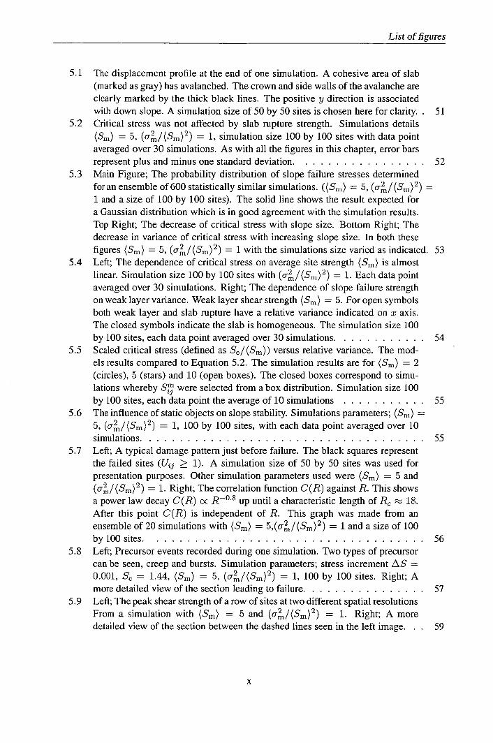
5.1 The displacement profile at the end of one simulation. A cohesive area of slab (marked as gray) has avalanched. The crown and side walls of the avalanche are clearly marked by the thick black lines. The positive y direction is associated with down slope. A simulation size of 50 by 50 sites is chosen here for clarity. . 51
5.2 Critical stress was not affected by slab rupture strength. Simulations details (Sm ) = 5, (o i /(Sm ) 2 ) = 1, simulation size 100 by 100 sites with data point averaged over 30 simulations. As with all the figures in this chapter, error bars represent plus and minus one standard deviation . . . . . . . . . . . . . . . . . 52
5.3 Main Figure; The probability distribution of slope failure stresses determined for an ensemble of 600 statistically similar simulations. ((S,,,) = 5, (o/(Sm ) 2 ) = 1 and a size of 100 by 100 sites). The solid line shows the result expected for a Gaussian distribution which is in good agreement with the simulation results. Top Right; The decrease of critical stress with slope size. Bottom Right; The decrease in variance of critical stress with increasing slope size. In both these figures (Sm ) = 5, (o/(S m ) 2 ) = 1 with the simulations size varied as indicated. 53
5.4 Left; The dependence of critical stress on average site strength (S m ) is almost linear. Simulation size 100 by 100 sites with (o i /(Sm ) 2 ) = 1. Each data point averaged over 30 simulations. Right; The dependence of slope failure strength on weak layer variance. Weak layer shear strength (Sm) = 5. For open symbols both weak layer and slab rupture have a relative variance indicated on x axis. The closed symbols indicate the slab is homogeneous. The simulation size 100 by 100 sites, each data point averaged over 30 simulations . . . . . . . . . . . . 54
5.5 Scaled critical stress (defined as S c /(Sm )) versus relative variance. The mod- els results compared to Equation 5.2. The simulation results are for (S m ) = 2 (circles), 5 (stars) and 10 (open boxes). The closed boxes correspond to simu- lations whereby Sim, were selected from a box distribution. Simulation size 100 by 100 sites, each data point the average of 10 simulations ........... 55
5.6 The influence of static objects on slope stability. Simulations parameters; (Sm) = 5, ( 0,2 /(Sm)2) = 1, 100 by 100 sites, with each data point averaged over 10 simulations . . . . . . . . . . . . . . . . . . . . . . . . . . . . . . . . . . . . . 55
5.7 Left; A typical damage pattern just before failure. The black squares represent the failed sites (Uij > 1). A simulation size of 50 by 50 sites was used for presentation purposes. Other simulation parameters used were (Sm) = 5 and (ali /(Sm ) 2 ) = 1. Right; The correlation function C(R) against R. This shows a power law decay C(R) x R 08 up until a characteristic length of R 18. After this point C(R) is independent of R. This graph was made from an ensemble of 20 simulations with (Sm) = 5,(0
7/(Sm ) 2 ) = 1 and a size of 100
by 100 sites ....................................56 5.8 Left; Precursor events recorded during one simulation. Two types of precursor
can be seen, creep and bursts. Simulation parameters; stress increment AS = 0.001, S = 1.44, (Sm) = 5, (0 i /(Sm ) 2 ) = 1, 100 by 100 sites. Right; A more detailed view of the section leading to failure . . . . . . . . . . . . . . . . 57
5.9 Left; The peak shear strength of a row of sites at two different spatial resolutions From a simulation with (Sm) = 5 and (0-2
m
I(SM)2) = 1. Right; A more detailed view of the section between the dashed lines seen in the left image. . 59

List of figures
5.10 The auto correlation function H(R) shows correlation up to the correlation length scale . results for resolutions of N = 4 and N = 12 are shown. Simulation parameters;(S m ) = 5 and (o i /(Sm ) 2 ) = 1. Data points averaged over 20 simulations . . . . . . . . . . . . . . . . . . . . . . . . . . . . . . . . 60
5.11 Left; The effect of increasing resolution on critical stress (when stress is scaled back to standard (N = 1) stress units) Right; The effect of the cos 2 interpola- tion technique on the relative variance the weak layer shear strengths. For both figures (Sm ) 5, (/(Sm ) 2 ) = 1, simulation size 100 by 100 sites, and the results averaged over 20 simulations . . . . . . . . . . . . . . . . . . . . . . . . 61
5.12 Varying correlation length while keeping all other variables constant has a strong knock down effect on slab stability. Simulation parameters (S m ) = 5, (a/(Sm ) 2 ) = 1, simulation size 100 by 100 sites with each data point being averaged over 10 simulations . . . . . . . . . . . . . . . . . . . . . . . . . . . 62
5.13 Left; An example of the strength fluctuations of a weak site in the time de- pendent model (W = 0.1). Right; The change in critical stress with different values. Simulation parameters (Sm) = 5, (0.2
m /(Sm)2) = 1 simulation size 100
by 100 sites. The data points in the right figure are averaged over 50 simula- tions. As with the other figures the error bars show plus and minus one standard deviation . . . . . . . . . . . . . . . . . . . . . . . . . . . . . . . . . . . . . . 63
5.14 Evolution of internal stresses a different percentages of the failure stress; (a)
5ext = 58% of S, (b)S t = 71% of sc, (c) 5ext = 84% of 5, (d) 5ext = 97% of S. Failure stress S = 1.55. Darker colours correspond to areas of negative stress, and lighter colours to positive stress. Simulation parameters
(Sm) = 5, (,7 2 I(Sm)l) = 1, simulation size 30 by 30 sites . . . . . . . . . . . . 64 5.15 The displacement profile of the primed slope. The external stress is 1.3 units.
The dark area represent large displacements. Simulation parameters; (Sm) = 5, (0 i /(Sm ) 2 ) = 1, 30 by 30 sites . . . . . . . . . . . . . . . . . . . . . . . . . . 67
5.16 The distribution of hotspots on a primed slope (same slope as in Figure 5.15). Regions where local damage caused global failure are marked in black. Re- gions where local basal damage weakened the slope, but not enough for failure to occur are dark grey. Finally regions where the damage did not alter slope stability (or in some cases even strengthened the slope) are light grey ...... 67
5.17 Left; For the non homogeneous slab at a relative variance of one, the avalanche sizes were approximately 40 percent smaller than if the slab were homoge- neous. The solid line shows the theoretical results (Equation 4.41). Simulation parameters; (Sm) = 5 and (O i /(Sm ) 2 ) = 1. A simulation size of 200 by 200 sites was used so that the avalanche area was not affected by simulation size. Error bars represent plus and minus one standard deviation. Right; Variabil- ity within the weak layer had a weak effect on the avalanche size. However variability within the slab had a strong knock down effect on avalanche size. Simulation parameters; (Sm) = 5, (5'!") = 10, size of 100 by 100 sites. . . 68
5.18 Left graph; The effect of notches on avalanche area. Right graph; The effect of notches on critical stress. In both case (Sm) = 5, with a simulation size of 100 by 100 sites. Data points averaged over 30 simulations . . . . . . . . . . . . . . 69
xi

List of
5.19 Shown are 1000 data points drawn from the distribution P(d - d') = (d - d') 038 - 1. We use this is approximate the exceedence probability distribution observed for real slab depths of P(> (d - d')) o (d - d') 26 (shown by the solid line) for (d - d') > 0.5, with a flattening of the curve below this value. 70
5.20 The exceedence size distribution of avalanche area for an ensemble of 240 sim-ulations. The solid line shows power law function P(> A) oc A l2 reported for a large ensemble of slab avalanches . . . . . . . . . . . . . . . . . . . . . . 71
6.1 The three different modes of fracture . . . . . . . . . . . . . . . . . . . . . . . 76 6.2 Linear elastic fracture mechanics considers a crack of length 2a which is under
a uniform stress o and is significantly larger than the non elastic zones found at the crack tips . . . . . . . . . . . . . . . . . . . . . . . . . . . . . . . . . . . . 77
6.3 Mode I device; Snow was carefully inserted into two hinged box sections. One section was attached to the table, and a weight was hung off the second section a distance J from the hinge. The snow in the gap between the box sections was cut until failure occurred .. . . . . . . . . . . . . . . . . . . . . . . . . . . 80
6.4 The mode I experiment. Left; Cutting through the snow block at the gap be- tween the box sections with a wire. Right; The device and fracture surface after failure. Although not apparent in this image, the fracture surface is rough, easily distinguishable from the surface caused by the cutting with the wire. . 81
6.5 The Tada relation we quote was developed for a three point bending test. Our situation is essentially an upside down three point bending test . . . . . . . . . 82
6.6 A cube of snow was carefully inserted into a section of square pipe which was split down the middle. One section was attached to the table, and a weight was placed on the other section. String was then used to cut along the snow at the join of the boxes until mode III failure occurs . . . . . . . . . . . . . . . . . . . 83
6.7 The mode III experiment. Left; Cutting through the snow block with a the string. In this picture the weak layer is being tested. The snow block had to be trimmed so that the weak layer coincided with the cutting plane. In the homogeneous tests the snow sample would fit better into the test device. Right; The device immediately after failure . . . . . . . . . . . . . . . . . . . . . . . . 84
6.8 The fracture surface associated with mode III failure. The vertical groove was added after to distinguish the cut from the fractured area . . . . . . . . . . . . . 84
6.9 The Mode III Tada relation for a crack beam with a shear force r acting parallel to the crack front (into the page) . . . . . . . . . . . . . . . . . . . . . . . . . . 85
6.10 The mode II device. One end of the device had no floor to allow for mode II failure. A barrier at the end of the box is closed to prevent mode I failure. . . 86
6.11 The mode II experiment. Left; Cutting through the snow block with string. Right; The device and fracture surface after failure. The fracture tends to cut into the snow block. This indicates that there is a mode I component to the failure 86
6.12 The mode III device was used to test in mode II. In this case a saw was used cut downwards through the block of snow until failure . . . . . . . . . . . . . . . . 87
6.13 The Mode II Tada relation was developed a cracked specimen where the stress r acts parallel to the crack . . . . . . . . . . . . . . . . . . . . . . . . . . . . . 88
6.14 The 41 mode I measurements. Averaging the 35 results with a valid cut depth gave critical stress intensity of 1480 Pa m 112................... 89
xli

List of figures
6.15 The 56 mode ifi results. These level off above a peak stress of approximately a/h 0.6 which corresponds to a peak stress of about 8000Pa. Averaging the 14 results above this turnover gave a critical stress intensity factor of 2190 ± 160Pa m 112.................................... 89
6.16 The 86 mode II results measured using the mode H device. The 7 very large results and those with a relative cut depth of less that 0.6 (which corresponds to a stress of between 2000 Pa and 3000 Pa) were discounted from this analysis. 91
6.17 The 33 mode II stress intensity measurements taken using the mode III device 92 6.18 Layers have an influence on the Mode II stress intensity. By fitting linear rela-
tions to the data the toughness parallel to the layering is found to be approxi- mately 85% of that perpendicular to the layering . . . . . . . . . . . . . . . . . 93
6.19 Layers also have an influence on the Mode ifi stress intensity of snow. By fitting curves to the data the mode ifi stress intensity parallel to the layers is found to be 75 % of that perpendicular to the layers . . . . . . . . . . . . . . . . 94
6.20 The stress intensity of the two weak layers was very similar. The values level off above a stress of approximately 3500 Pa. This corresponds to a relative cut depth of around 0.6. The mean value of the 13 results with a relative cut depth of less than 0.6 was 1000 Pa m 112......................... 95
6.21 The friction device; The mode III device was attached on its side to the table. A shear stress of 2500 Pa m 112 was produced with a pulley and a 5kg weight. Normal stresses were produced by placing weights on top of the device. . . . . 96
6.22 Results of friction experiment. The normal stress varied between 0 Pa and 4350 Pa. Shown are results of Equation 6.17 with three different values of JL. These are 0.3 (dashed line), 0.4 (solid line) and 0.5 (dotted line) . . . . . . . . . . . . . 98
7.1 A shear band is an extended length or area of half length/radius 1, where the shear strength of the weak layer has dropped of to its residual frictional value Tr 102
7.2 The variation in critical flaw size with slope angle should friction be ignored and j = 0. 5, as predicted by the Griffith relation. If p = 0.5 then critical shear band size diverged for a slope angle of 27 degrees .. . . . . . . . . . . . . . . . 104
7.3 The variation of critical flaw size with slope angle. The dotted line shows the one dimensional critical half length as predicted by the Griffith relation (Equa- tion 7.4. The solid line is critical shear band radius of the thin slab approxima- tion (Equation 7.13)................................ 107
7.4 A schematic of a solitary wave. Compressive failure of the weak layer creates a solitary wave which propagates along the slab/weak layer ........... 109
7.5 The energy released by a solitary wave and a shear band assuming various "standard" parameters (see test for details). The solitary wave has a smaller energy barrier, and critical size ........................... 111
xiii

List of tables
9.1 Typical values and ranges of the physical parameters entering the model . . . . 119
10.1 A brief description of the snow used for the fracture toughness experiments. Hardness as defined by the hand hardness index. For Density the mean value is given in the first line, and the maximum and minimum values measured for that snow are given in brackets. For mode one critical stress intensity (KJQ) the mean plus and minus one standard deviation is given. In the final column which tests, and how many were carried out is listed . . . . . . . . . . . . . . . 120
xiv

Acronyms and abbreviations
LEFM Linear Elastic Fracture Mechanics
SLF Schnee-und Lawinenforschung
Soc Self Organised Criticality
CA Cellular Automaton
xv

Nomenclature
a Cut depth/crack half length
A Avalanche area
A Non Dimensional acceleration
C(R) Damage correlation function
Ct Time step parameter
d Height of snow on ground
d' Height of weak layer
Ad Change in d due to weak layer collapse
D Sample Size
D0 Characteristic size
E Young's Modulus of material
g Terrestrial gravity
G Shear Modulus of material
h Specimen height
H(R) Strength correlation function
I Stress redistribution factor
J Beam length
J Horizontal distance from hinge to weight
K Fracture toughness
KQ Stress Intensity factor
Kapp Apparent fracture toughness
I Dimensional shear band radius or half length
L Non Dimensional shear band radius or half length
M Moment per specimen width
N Resolution of model
P Specimen beam width
xv'

Nomenclature
R Non Dimensional Radius/distance
S Non Dimensional stress
Sc Critical (slope failure) shear stress
(Se ) Mean Critical shear stress
Sm Peak weak layer shear strength
SR Rupture strength of slab
(Sm ) Mean peak shear strength
SI/TI Slab rupture strength
t Dimensional time
T Non Dimensional time
W General displacement field
W Mass of suspended weight
U Dimensional displacement
U Non Dimensional displacement coordinate
v Dimensional velocity
V Non Dimensional velocity coordinate
x Dimensional across slope coordinate
X Non Dimensional across slope coordinate
Y Dimensional down slope coordinate
Y Non Dimensional down slope coordinate
z Dimensional out of plane of snow coordinate
Surface energy
0 Slope angle
Coefficient of friction
V Poisson's ratio
Correlation length
P Snow density
a General stress tensor
UN Normal stress
U2 Variance of peak shear strength
r Dimensional shear stress
TM Dimensional peak shear strength
Tr Residual shear strength
v Characteristic displacement xvii

Chapter 1 Introduction
Snow avalanches are a major natural hazard. They threaten people and property in mountainous
regions throughout the world. The average number of snow avalanche fatalities worldwide is
estimated at 250 per year [1]. During the last century the number of victims in buildings or on
roads has decreased due to better hazard evaluation and understanding of avalanches. However,
the number of recreational accidents has increased, mainly due to the huge increase in the
popularity of winter sports. The number of accidents is still low compared to the number of
people taking part in snow sports. This is due to avalanche education and improved avalanche
forecasting.
- .
-.
.d-I J..
:'c' ••.•r•
- -
p.. .
Figure 1.1: A real slab avalanche, in this case the weak layer has been the interface with the bed rock. Photo: A. Fyffe
In general, there are two types of snow avalanches; loose snow and slab avalanches. The initial
failure of a loose snow avalanche is similar to the rotational failure of cohesionless sand or soil.

Introduction
but generally occurs with a smaller volume of material [1]. The failure begins at a point and
spreads out down slope in an inverted V shape. A slab avalanche on the other hand occurs when
a cohesive slab of snow slides on a weak layer (Figure 1.1). The observed ratio between the
width and thickness of the slab varies between about 10 and 1000 to 1, with the slab thickness
generally being < I [1]. Slab avalanches can consist of either wet or dry snow. Dry snow slab
avalanches represent the main avalanche hazard because they tend to be larger, more common
and less predictable than other forms of avalanche. Jamieson and Johnston [2] report that
between 1972 and 2000, 99% of avalanche fatalities in Canada were due to slab avalanches.
Due to the regular occurrence of this type of avalanche, much qualitative field information has
been collected.
Slab avalanches are common due to the typically highly layered nature of a mountain snowpack.
The first stage in the creation of this snowpack is the formation of snow flakes via the deposition
of super-cooled water vapour onto dust and other particles. The shape of the crystals depends on
the conditions (temperature, humidity, etc.) they form in. The most common form is the classic
"christmas card" dendrite (see Figure 1.2). If these snow flakes fall in cold, calm conditions
they form a low density network of crystals commonly called powder snow. If they fall in
windy conditions, which are common in mountainous regions, they tend to get broken up, and
the fragments packed together to form wind slab. Once on the ground, temperature changes
and metamorphic processes continue to modify the snow. Storm cycles and changing weather
conditions build up a highly layered mountain snowpack. Within the snowpack some layers
will have greater shear strength than others, and in some cases the bonding between adjacent
layers (or with the ground) may be weak. The presence of such weak layers is necessary, but
not sufficient, for the production of slab avalanches.
For a slab avalanche to release, five different forms of failure are necessary. These are; shear
failure in the weak layer (basal failure), tensile fracture at the up hill side of the slab (crown
wall), compressive failure at the down hill side of the slab (stauch wall), and two lateral cracks
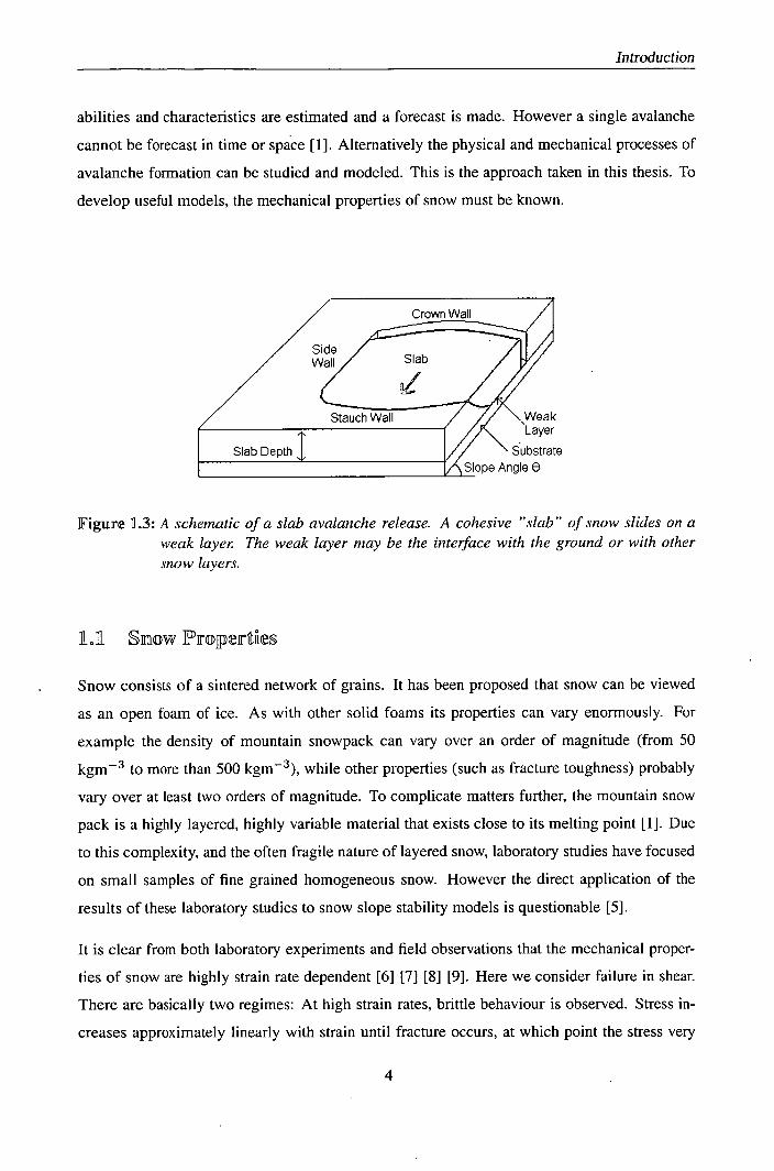
at the sides of the slab (side walls). Figure 1.3 is a schematic diagram of slab avalanche release.
It is generally accepted that release begins with basal shear failure [3] (in this thesis "basal"
means the base of the slab, rather than necessarily the base of the snowpack).
Slab avalanche release can occur in two ways. They can occur spontaneously due to either
increased load (from additional snow fall), or due to changes in snowpack properties. Alter-
natively release can be triggered by the addition of an external load. Common examples of
2

4
4b4 JJ
Introduction
4f!1 - ,•. ,_.J .,. .;•
:
Figure 1.2: Low temperature scanning electron microscope pictures of snow. Left, a classical, dendrite shaped, snowflake captured just after landing on the ground. Right; Small rounded particles fbrmed by the fragmentation and metamorphism of snow flakes. This is typical of the snow that produces slab avalanches. Photos; Blair Fyffe and Chris Jeffrees
an external load are a skier or an explosive charge. The majority of slab avalanches release
spontaneously during storms. Generally these are less of a hazard to recreational ists as there
tends to be fewer people in avalanche terrain during such periods. The majority of recreational
avalanche accidents are externally triggered by the victim [3].
There are two forms of external triggering; direct and remote. A direct avalanche occurs when
the trigger causes the slope that he/she/it is on to release. Remote triggering occurs when the
trigger is not located within the area that initially fails. Indirect avalanches can be associated
with whumpfs. A whumpf occurs when a weak layer collapses under the weight of the over-
laying snowpack, and the slab settles vertically downwards. The name comes from the fact that
as the fracture propagates, a distinct "whumpf" sound can often be heard. On some occasions
the snowpack can be seen or felt to displace downwards. An example of a whumpf causing an
indirect avalanche is reported by Bruce Jamieson [4]. When skiing with friends in the Purcell
mountains, they heard and felt a whumpf. Four hundred metres to their side a large avalanche
released. After investigation of the snow they came to the conclusion that despite the snow
being stable where they were, they had created a fracture which had traveled 400 metres before
initiating the avalanche.
In general two approaches have been taken for studying avalanche release. The first is a statisti-
cal approach. This is the technique used by most avalanche forecasting services. By empirically
weighting the influence of the contributing factors for a specific situation, the avalanche prob-
3

Introduction
abilities and characteristics are estimated and a forecast is made. However a single avalanche
cannot be forecast in time or space [1]. Alternatively the physical and mechanical processes of
avalanche formation can be studied and modeled. This is the approach taken in this thesis. To
develop useful models,' the mechanical properties of snow must be known.
Crown Wall
Side / Wall / Slab (7
Stauch Wall / // \Weak
Slab Depth '
Substrate Slope Angle e
Figure 1.3: A schematic of a slab avalanche release. A cohesive "slab" of snow slides on a weak layer The weak layer may be the interface with the ground or with other snow layers.
1J Snow TPrcrDJpertes
Snow consists of a sintered network of grains. It has been proposed that snow can be viewed
as an open foam of ice. As with other solid foams its properties can vary enormously. For
example the density of mountain snowpack can vary over an order of magnitude (from 50
kgm 3 to more than 500 kgm 3 ), while other properties (such as fracture toughness) probably
vary over at least two orders of magnitude. To complicate matters fui:ther, the mountain snow
pack is a highly layered, highly variable material that exists close to its melting point [1]. Due
to this complexity, and the often fragile nature of layered snow, laboratory studies have focused
on small samples of fine grained homogeneous snow. However the direct application of the
results of these laboratory studies to snow slope stability models is questionable [5].
It is clear from both laboratory experiments and field observations that the mechanical proper-
ties of snow are highly strain rate dependent [6] [7] [8] [9]. Here we consider failure in shear.
There are basically two regimes: At high strain rates, brittle behaviour is observed. Stress in-
creases approximately linearly with strain until fracture occurs, at which point the stress very
4
Introduction
abilities and characteristics are estimated and a forecast is made. However a single avalanche
cannot be forecast in time or space [1]. Alternatively the physical and mechanical processes of
avalanche formation can be studied and modeled. This is the approach taken in this thesis. To
develop useful models, the mechanical properties of snow must be known.
Crown Wall
Sla
Wall b
Stauch Wall
Side
'Weak Layer
Slab Depth Substrate Slope Angle 0
Figure 1.3: A schematic of a slab avalanche release. A cohesive "slab" of snow slides on a weak layer The weak layer may be the interface with the ground or with other snow layers.
LII Sllhl©w Properties
Snow consists of a sintered network of grains. It has been proposed that snow can be viewed
as an open foam of ice. As with other solid foams its properties can vary enormously. For
example the density of mountain snowpack can vary over an order of magnitude (from 50
kgm 3 to more than 500 kgm 3 ), while other properties (such as fracture toughness) probably
vary over at least two orders of magnitude. To complicate matters further, the mountain snow
pack is a highly layered, highly variable material that exists close to its melting point [1]. Due
to this complexity, and the often fragile nature of layered snow, laboratory studies have focused
on small samples of fine grained homogeneous snow. However the direct application of the
results of these laboratory studies to snow slope stability models is questionable [5].
It is clear from both laboratory experiments and field observations that the mechanical proper -
ties of snow are highly strain rate dependent [6] [7] [8] [9]. Here we consider failure in shear.
There are basically two regimes: At high strain rates, brittle behaviour is observed. Stress in-
creases approximately linearly with strain until fracture occurs, at which point the stress very
4

Introduction
rapidly drops to a residual frictional value. At lower strain rates ductile failure is observed
Again stress initially increases linearly with strain. However a peak value is soon reached, af-
ter which the stress decreases with strain to eventually reach a residual frictional value. The
transition between these two regimes occurs at about 10 - 10 4 s 1 .
It has been argued that these results can be explained by the fast metamorphism, i.e. the re-
welding of broken bonds during testing [9]. When the strain rate is low, the bonds can regen-
erate after their destruction, while at higher strain rates they do not have the opportunity to do
this. Louchet [10] developed a theoretical model of slope stability allowing for bond rupture
and re-welding. This model predicts a ductile to brittle transition.
The brittle behaviour observed at high strain rates implies that fracture toughness, and not shear
strength may be the fundamental quantity relating to instability. Fracture toughness defines the
ability of a material to sustain stresses in the presence of localised flaws/cracks. There are
three forms or modes of fracture. Mode I failure is in tension, meaning the stress is opening
the crack (see Figure 1.4). Mode II is in plane shear, then the displacement associated with
the crack is in the same direction as crack tip propagation. Finally mode III is antiplane shear,
when the displacement is perpendicular to the crack tip propagation. Each of these modes is
associated with a different value of fracture toughness. The majority of experimental work on
the fracture toughness of snow has concentrated on the mode I value. The technique used to
measure this involves harvesting a beam of snow with a rectangular section of metal piping.
The pipe section is then held horizontally while the beam of snow it contains is pushed out a
predetermined length. This cantilever of snow is then carefully cut from the top until it snaps
under its own weight. By measuring the mass of snow which has broken off, and the depth of
the cut at fracture, the fracture toughness in mode I can be calculated. Such experiments were
carried out by Kirchner et al. [11], and Faillettaz et al. [12]. Values of between about 0.1 and
1.5 kPa m112 were obtained depending on the snow type and density. These are incredibly low
values of fracture toughness, suggesting that snow is one of the most brittle materials known to
man.
However an unexpected dependence of fracture toughness on cantilever length was reported by
Faillettaz et al. [12]. Furthermore, the sample sizes were not large enough to obey the theory
of linear elastic fracture mechanics [13]. In 2005 (during which time this thesis was being
produced) Sigrist et al. [5] investigated to what extent fracture toughness values were affected
by specimen size and shape. Geometry specific analysis techniques and size corrections were

Introduction
Mcdei Mode 11 Mode U1
Figure 1.4: The three modes offailure.
developed, which gave fracture toughness values which were larger than those reported by
earlier researchers.
1.2 Medliuiinicall Models
The simplest stability model compares the shear strength of the weak layer to the shear stress
due to the overlaying slab and any additional near surface loads. The ratio of stress to strength
is called the stability index [14] [15]. This model implies that avalanches will release when
the stability index exceeds one. The concept of a stability index has proved useful for human
triggered avalanches, and in part for snow storm avalanches, but is of little use for most other
natural avalanches [1].
However, the strain rates involved in avalanche release are high, and failure is a brittle process.
This means that the release process is governed by fracture mechanics, and a simple stress
criterion is insufficient or even inappropriate for avalanche release. Fracture mechanics was
first applied to geophysical phenomena by Palmer and Rice [16] in their classic paper of 1973
on the failure of over-consolidated clay slopes. They reported that a shear band is initiated at
a stress concentration, and a slow strain softening at the tip of the band follows until a critical
length is reached. The cause of the initial stress concentration and the mechanism of subsequent
slow propagation are not clear. The band then propagates rapidly and the slope fails. This model
is fairly general to any strain softening material, and was applied to the avalanche problem by
McClung [17] [18].

Introduction
Most models of slab avalanche release assume the existence of some form of deficit zone or
shear band within the weak layer. Schweizer [3] considers in some detail the critical shear
band size. Assuming standard snow parameters and given a reasonable estimate of friction, for
ductile failure he finds this to be between 1 and 3 metres. For brittle failure he obtains a value
between 3 and 8 metres.
One problem with all these models is that the technique (the J-integral technique) used to derive
the condition for the rapid propagation of the shear band is only applicable to very simplified
quasi-one-dimensional shear band geometries. The fact that many of the parameters associ-
ated with slab avalanche release are not well known due to the highly complex and variable
properties of snow further complicates Schweizer's predictions.
Several authors [19] [20] [21] report that variations in the shear strength of weak layers are an
almost generic feature of avalanche prone slopes. Birkeland et al. [22] found that there exists a
significant relationship between snow depth and average snow resistance in some areas. How-
ever in an area of more complex terrain and less localised wind drifting, no such relationship
existed. Instead a complex pattern of resistance demonstrated that many factors contribute the
distribution of snow properties. Conway and Abrahamson [20] attempted to evaluated stability
by determining the probability of finding deficit zones where the shear strength falls below the
acting gravitational stress. However this approach has the problem that the overlaying slab may
redistribute stress from weak areas to stronger neighbouring regions. Also, in the presence of
local strength variations the situation may be further complicated by the presence of multiple
flaws, which lead to complex stress redistribution patterns.
This shows that slope stability is dependent on more than average weak layer shear strength.
Variations in weak layer shear strength, and the length scale of this variation are relevant to
this problem. The relation between these three parameters and slope stability is likely to be
complex.
In common with many other forms of slope failure like land slides and rock falls, snow avalanches
show a power law size distribution. This means that the probability of an event being larger than
size/area A is proportional to A to a minus power; P(> A) 0C A. For snow avalanches the
power law exponent y is about 1.2, independent of the triggering mechanism [23].
When investigating fallen slab avalanches, McClung [24] found that slab depth was also power
law distributed, and that weak layer shear strength showed a dependence on slab depth. The
7

Introduction
shear strength increased with slab depth due to greater creep and normal pressure. He concluded
that the power law distribution of slab avalanches reflects the power law distribution of the
controlling parameters (shear strength).
Another possible cause of this power law distribution is self organised criticality (SOC) or
some form of related critical phenomenon. The concept of SOC was first developed by Bak et
al. [25] using sandpile models. This theory predicts a power law distribution of avalanche sizes
in these sandpiles. However, in real sandpile experiments power law size distributions were not
observed. This was due to inertial effects. If the same experiments were carried out using a less
dense material such as rice, then power law size distributions would be observed.
2.3 Computer Modells
An early computer model of snow slab failure was developed by Aström and Timonen [26].
Their model investigated the influence of statistical variations of strength. They used a basic
finite element technique to discretise the snow slab. The slab was modeled as a series of points
connected via a two dimensional network of beams. These were connected to the ground via
other beams. The beams would fail in both shear and tension when the stress acting upon
them reached a threshold value. They found the grade of heterogeneity of the bonding of the
snow to the ground and the ratio of this value to the slab fracture threshold to be the important
parameters for fracture behaviour. Although this model was neither realistic nor supported by
data, it showed that the consideration of strength variation is important.
The cellular automaton (CA) method provides a numerically simple and efficient way to model
and simulate a complex physical process by considering a description at the level of the basic
components of the system. The CA technique considers space, time and all physical quantities
to be discrete. In addition, the time evolution is applied synchronously to all spatial points.
The state of each discrete sits from generation to generation is determined by a simple set of
rules relating to the state of the site and that of the surrounding sites. Although these rules are
very simple and take only the essential features of the real interactions are taken into account,
it is observed that the collective behaviour that emerges from the CA dynamics is identical,
in the appropriate limit, to the real phenomenon. It is found that over-simplified microscopic
modelling provides an accurate description of the macroscopic level is a common feature of
many complex systems.

Introduction
The cellular automaton approach has been very successful at modelling many diverse processes
in physics and related domains. In the field of natural hazards they have been successfully
applied to earthquakes, landslides and forest fires.
A very simple one dimensional CA model of slope stability which aimed to investigate the
influence of variability was developed by Zaiser [27]. In this thesis we generalise this sim-
ple model into two dimensions and introduce many different influences. However this simple
model provides the basic structure for all our computer simulations.
At the same time as this thesis was being written Faillettaz et al. [23] developed a two dimen-
sional cellular automaton model of avalanche release. The motivation was to investigate the
cause of the power law size distribution of slab avalanches observed in field data. The basic
structure of this model is similar to that of the model we develop in this thesis. Common as-
pects are that stresses can be re-distributed via the non-uniform displacement field, and failure
can occur in both shear and tension. However in other aspects their model is simpler than ours:
in shear they assume a rupture strength rather than the displacement softening behaviour that
we assume, and they do not consider inertial effects. Their main result is that if both the shear
and tensile strengths are allowed to vary randomly, then a power law size distribution can be
obtained. By tuning the ratio of average shear to tensile strength, the exponent of this power
law distribution could be varied. They concluded that the underlying cause of the power law
distribution was some kind to critical phenomena, and that the exponent of the power law in
some way represents the material anisotropy.
Recently Kronholm and Birkeland [28] used a slightly modified version of the model we de-
velop in this thesis to investigate the relation between the scale of the spatial variability and
slope stability. They implemented the spatial variability in a different way to that described
here. However their conclusions were the same; the length scale of the spatial variability has a
strong knock down effect on slope stability.
14 Afls and Obctives of this Thesis
In the first part of this thesis a two-dimensional version of the Palmer Rice model, which is
able to take into account the inhomogeneity reported by many authors, is developed and in-
vestigated. This involves a generalisation the original Zaiser problem. The aim of this is to
bridge the gap between the simplified analytical solutions and the qualitative observations of

Introduction
field workers. It is important to emphasize that this model does not aim to capture all the
physical details of slab failure - rather, a simplified model is used to assess the influence of
certain variables and parameters, such as variability and rupture strength, in a qualitative and
semi-quantitative manner. The results may be useful to put information that is already known
- such as the fact that variability reduces slope stability - on a firmer theoretical footing. The
model is developed by considering snow properties and behaviour in Chapter 2. The simulation
technique is developed in Chapter 3. The work in detailed in these two chapters was derived
either by or in conjunction with various other authors) with In Chapter 4 the models results
are compared to analytical solutions. In Chapter 5 the results of the model for more complex
(realistic) situations are reported. These results derived by myself and as well as being quoted
here are described in three journal articles [29] [30] [31].
The design and implementation of a series of experiments which aimed to measure the three
different modes of fracture toughness of wind slab are reported in Chapter 6. The aim was to
achieve size independent values of fracture toughness that could be directly applied to larger
scale avalanche models. These experiments were carried out using specially designed boxes.
Also investigated were the effects of friction within the system. The results were analysed in a
geometry specific manner, and adjusted to account for the relatively small size of the cantilever
beams, using a method suggested by Sigrist et al. [5].
Finally, in Chapter 7 results from both the modelling and experimental parts of this work are
brought together to critically discuss different release models for slab avalanches.
10

Chapter Snow i1\ I)U r
As stated in the Introduction, slab avalanche release is essentially a fracture mechanics problem.
To a first approximation we assume that the material surrounding the weak layer behaves like a
linear elastic material. In this sense, characterising the state of a slope prior to avalanche release
involves the solution of an elastostatic problem. After specifying the geometry of an idealized
slope in Section 2. 1, the solution of this elastic problem is discussed in Section 2.2. Avalanche
release occurs by shear failure of a weak layer in the snowpack and will entail tensile and shear
failure of the slab. The corresponding assumptions about material properties of the slab and the
weak layer are detailed in Section 2.3. Finally, after release of the avalanche, inertial effects
may come into play and affect the avalanche size. Modifications of the model for this dynamic
case are discussed in Section 2.4.
21 M©dleli Geometry
In our model of slab avalanche release, a simplified three-layer model of the unstable snowpack
(of total depth d) on an avalanche-prone slope (see Figure 2.1) is considered. The across and
down slope directions are associated with the x and y directions of a Cartesian coordinate
system and the z direction is perpendicular to the plane of the weak layer. A weak layer is
found on the plane z = d'. A cohesive slab of depth (d - d') overlays this weak layer. The
slab, as well as the snow below the weak layer, are modeled as homogeneous linearly elastic
media. Finally, the bottom of the snowpack adheres to the bedrock which is considered of
infinite stiffness. The weak layer may coincide with the interface between the snowpack and
the bedrock (d' = 0). As shown in Section 2.2, this does not affect the results, which only
depend on the thickness of the slab above the weak layer. This snowpack is found on a slope
inclined at an angle 9. A uniform shear stress of pg(d - d') sin 9 acts upon the weak layer due
to the slope parallel component of the slab's weight. This is referred to as the external stress
Text. The term external is used because, as opposed to the internal stresses discussed below, it
stems from the external action of gravity on the system rather than from the internal state of the
stratified snowpack.
11

Snow Behaviour
k Layer
Figure 2.11: Snowpack geometry considered in the model. The x direction will be out of the
plane of the page. It is later shown that the value d' does not influence the results, and so this is set to zero.
The weak layer may exhibit heterogeneities in the form of strong and weak regions, or of
interface cracks. Weaker regions are more likely to displace downslope in response to the
external stress than stronger regions. This may produce a non uniform displacement field across
the weak layer u(x, y), where u is defined as the displacement of the slab in the down slope
direction. Some areas of the slab are squashed while others are stretched. The slab is a linear
elastic material and so will produce stresses to accommodate the non uniform displacement
field. These internal stresses 'Tint will in turn, modify the shear stress which acts on the weak
layer. Internal stresses will act in such a manner that regions of larger displacement (weaker
areas) are supported by less displaced regions (stronger areas).
22 The Ellastflc Response
An expression for the internal stress field produced by a general displacement field has to be
found. In this thesis two derivations are given. A less rigorous but more intuitive two dimen-
sional argument as derived by Zaiser [27] is given first (Section 2.2.1). The results of this can be
generalised into three dimensions in a heuristic manner. Then a second, rigorous three dimen-
12

Snow Behaviour
sional argument which confirms the heuristic approach is given in Section 2.2.2 (this section
was derived in conjunction with various other authors see [32]).
2.2.1 Two Dimensional Modell and Phenomenological Generalization
In this section an expression for the internal shear stress of the weak layer is derived in a two
dimensional setting. The two dimensions considered are the x and z dimensions. The results
are then heuristically generalised to three dimensions. The argument is based on a dislocation
representation of the stress field.
The internal stresses produced by a mode III crack are considered. A mode III crack implies
that the displacement of the slab (the y direction) is perpendicular to the direction of crack
propagation (the x direction). This is analogous to the situation where basal failure spreads out
across slope until slab failure occurs and the side walls of an avalanche are produced.
A slope that is totally homogeneous in the y direction (see Figure 2.2) is considered. Assume
that region 1, which is marked in grey, is displaced downslope. Assume that the surrounding
area (Region 2) is not displaced and does not deform. The misfit or deformation between the
two regions is concentrated into a narrow region at the boundary. This misfit is defined as a
dislocation. Due to the geometry of the situation these are two screw dislocations of opposite
sign. A cross section of this slope, and the associated displacement profile are also shown in
the right hand side of Figure 2.2.
A dislocation can be considered a unit displacement step. Any general displacement field can
be constructed from the superposition of unit displacement steps. Therefore any displacement
field can be constructed from an array of dislocations. The dislocation density of this array will
be equal to the derivative of the displacement field.
The internal stress field associated with a general displacement field can be found. Initially the
stress field generated by a single dislocation is considered. A dislocation will produce a stress
tensor. Only one component of this, the shear stress 'ru , acting on the plane z = d' is relevant
to the problem of slab avalanche release. 'r(x - x') is defined as the shear stress acting at a
general point x, due to a dislocation of unit strength located at point x ' .
By superimposing the stress fields of all the dislocations that produce the displacement field,
the stress field can be evaluated. Therefore the total stress at point x will the product of the field
13

Snow Behaviour
Figure 8
Figure x E
0
Region 2
{
I point point _____________________ b
a V
Figure Region 1
Region 2 - -------------Region 2 Slab
Region 1 1 Weak L; Layer
- - -: Ground
Figure 2.2: Figure A; Dislocations will be found at the boundary of regions 1 and 2. Figure B; The displacement profile of the cross section a - b. Uo implies no displacement has occured. Figure C, A cross section of the slab between points a and b. Two screw dislocations of opposite sign are found at the boundaries between regions I and 2.
of one dislocation (x - x') times the density of dislocations V'u(x') found at x', integrated
over all x' [27],
Tint (X) = - j -r(x - x')V'u(x')dx'
(2.1)
The stress field produced by one dislocation is complicated because the dislocation is contained
in a layer with elastic modulus E sandwiched between media with E 00 for z < 0 (the
bedrock) and E 0 for z > d (the open air). This defines the following boundary conditions.
The snow surface (z = d) is not in contact with anything solid, which implies that no shear
stresses will act here. The ground is considered infinitely stiff so there can be no displacement
here.
These boundary conditions can be incorporated using an array of dislocations. As any displace-
ment will be in the down slope (y) direction, any dislocations will have screw characteristics.
The displacement field of a screw dislocation in an infinite medium is antisymmetric, and the
stress field symmetric. A screw dislocation located at point (0, d') is considered. The shear
stress on the plane z = d can be canceled out (to satisfy the first boundary condition) by placing
a negative screw dislocation a distance d - d' above the free surface. This will be at z = 2d - d'.
This is called the zero order image dislocation. Then to satisfy the second boundary condition
two more dislocations are needed to compensate for the effects of the true dislocation and the
14

Snow Behaviour
zero-order image. As the displacement field is anti-symmetric, these are of the same sign as
the true dislocation and zero-order image. They are found at equal distance from, but on the
opposite side of the plane z = 0 as true and zero order image. This gives a positive dislocation
at z = —d' and a negative dislocation at z = —2d + d' (see Figure 2.3). To compensate for the
effects of positive dislocation at z = —d' and a negative dislocation at z = —2d + d' on the free
surface it is necessary to place reverse minor image of these through the plane z = d. The set
of four dislocations just discussed (found at z = —2d + d', z = —d, z = 2d and z = 2d - d')
are called the first order images. These last two dislocations will mean that again the z = 0
boundary condition is not satisfied, and so another two dislocations have to be added which will
violate the other boundary condition. The process is repeated infinitely often, each time placing
new dislocations through the planes z = 0 or z = d, with each set of images getting a distance
d further out. This gives image dislocations at ±2nd, —2(nd - d + d') and +2(nd + d - d')
where n is the order of the images.
The strength of a dislocation is defined as the displacement step (in a lattice this would cor-
respond to the Burgers vector). The shear stress due to a screw dislocation of unit strength is
given by I Gxwhere r is the distance from the dislocation and C the shear modulus of the weak
layer [33]. The true and zero order dislocation, which are located at z = d' and z = 2d - d',GX will produce shear stresses in the weak layer of T(x) = 2R-(x2) and T(X) = 2ir(x2 +4(d-d')2 )
I
Gx
respectively. Summing over the effects of the true dislocation, the zero order image and four
contributions for every order of images after that gives [33]
Gx 7 1 1
T (x) = - 2 + 4(d - d')2
(2.2)
- 2 1 1
+ -r I X 2 + 4(nd)2 - x 2 + 4(nd - d + d')2 - x 2 + 4(nd + d - d/)2 ]) n=1
An important approximation is now made, it is assumed that the snowpack is thin in the sense
that variations in n occur on a characteristic length scale which significantly exceeds d and d'.
It is then possible to expand the slowly varying function V'u(x') in a Taylor series around
= x: V'u(x') = Vu(x) + (x' - x)Vu(x) + .... Inserting this into Equation (2.1) gives
the first term
Tint - J r(x - x')Vu(x)dx' + f (X - x')r(x - x')Vu(x)dx + (2.3)
15

2(d-d')
d Z
¶TT: TI7; Slab
Weak Layer
. around
2 ( d- d')
Figure 2.3: The true dislocation is found at z = d'. The zero order dislocation is negative and is placed at z = 2d - d' so that the first boundary condition (traction free snow surface) is satisfied. Two first order dislocations are located at z = —d' and z = - (2d - d) to satisfy the second boundary condition (no displacement at ground surface) are shown. The other two first order dislocations, located at 2d and 2d - d' are not shown on the diagram.
The gradient terms can be taken outside the integral as they do not depend on x'. If this is done,
then the only expression left inside the first integral is r(x - x'). This is an odd function, and
so the first term vanishes and we get
Tint (x) where I = fxr(x)dx. (2.4)
Inserting Equation (2.3) into Equation (2.4) gives [33]
I Cx27 1 1
2 (2 - x 2 + 4(d - d')2 (2.5)
cc
+ [X2 + 4(nd) 2 - x 2 + 4(nd— d + d')2 - 2 + 4(nd+ d - dI)2]) dx.

Snow Behaviour
For clarity the first two terms in this expression (defined as IA) are considered separately to the
summation (defined as IB). The first two terms give
)dx 'A = f G (1_X2+4(dd,)2 C
= [x - x + 2(d - d') arctan (4(d - ) 100
= (d—d')G, (2.6)
while the summation gives
'OO
I 2x x2 x2
'B = J
((_i) x 2 +4(nd) 2 - x2+4(nd—d+d')2 - X2+4(fld+d_d/)2]) (2.7)
When this function is integrated it gives three arctan functions. As the limits of the integral are
plus and minus infinity these all give the same result (27r). In the equations below these arctan
functions are represented by the square brackets and not explicitly written down for the sake of
brevity. All the prefactors cancel out.
'B = (_1)(4nd[ ]-2(nd—d+d')[ ] 00 ] 00
G 00
=
= 0. (2.8)
The only contribution to the internal stresses are from the true dislocation and its zero order
image.
I = (d - d')C. (2.9)
The stress redistribution factor (I), is proportional to the thickness of the slab above the weak
layer but does not depend on the thickness of the underlying snowpack.
For displacement fields u(y) (plane shear) a similar procedure can be followed and the result is
of the same form as Equation 2.9. It can be assumed that in two dimensions the internal stress
is the sum of the one dimensional components.
752 a2u\ (2.10)
17

Snow Behaviour
i.e., the internal stress is proportional to the Laplacian of the displacement field. If any mixed
term (proportional to u) were present in the true solution, then this could always be eliminated
by a rigid rotation of the coordinate system. However it should be emphasised that at the present
stage Equation 2.10 is just a heuristic generalisation of Equation 2.4 to a two dimensional
displacement field. In the next section it is shown that I, the stress redistribution factor, is
different in the x and the y directions. However it is reassuring that the simple explanation
given above gives a solution of the same form as the one derived later in a more formal manner.
2.22 Three Dimensional Model
A more rigorous mathematical derivation of the elastic response to a displacement field is now
presented using energy arguments (see also [34]). Initially the elastic energy functional associ-
ated with a general displacement vector field w in an isotropic material is considered. This can
be written as [35]
Ee (W) = G [a(VW) 2 + (V x w)2] d3 r. (2.11)
The term a is a function of the Poisson ratio
(
ii
a = - 2zi)
(2.12)
The associated equilibrium equation is [35]
V2w + 1 _2V(Vw) = 0. (2.13)
This is solved by imposing along the z = d plane (weak layer) the condition that there is
no displacement in x or z directions (wx wz = 0), and w(x, y, d') = u(x, y). Strictly
speaking, this implies that the weak layer coincides with the bedrock, as the snow below the
weak layer is assumed not to deform. However as shown in the last section the same results are
recovered if a generic position of the weak layer is considered and u(x, y) is understood as a
discontinuity in w across the weak layer.
The equilibrium equation can be readily solved in Fourier space. The solution (in the long
18
Snow Behaviour
wavelength limit) which satisfies the imposed boundary conditions is given by (ref [Mor06])
' dk Y, z) = I (2)2 exp [i(k x x + ky) - (k + k)" 2 (z - d')] u(k, k) + Q(kz),
W z (X,y,Z) = O(kz) , wz(X,y,Z) = O(kz) . (2.14)
We now make the crucial assumption that the distance d - d' between the weak layer and
the surface of the slope is much smaller than the characteristic lengthscale of variations in
the displacement field: Ik(d - d')I << 1 where k is a characteristic wavevector of the stress
and displacement fields. This allows us to neglect the terms of order O(kz) and higher in the
displacement field.
The elastic energy functional (Equation 2.11) now becomes
E, (w) cf [C'
() + () + (p)] d3r. (2.15)
The elastic energy associated with the displacement field u(x, y) is obtained by inserting the
displacement field (Equation 2.14) into the energy relation (Equation 2.15). This gives a term
- from the first partial derivative, - from the second and - (k + k)w from the
third. Putting all this together gives
d2 k Ee (u) = _cff (27r)2 (( + 1)k + 2k)u(k, ky ) ei e__d'd3r. (2.16)
Now we integrate over the z coordinate from d' to d, in the long-wavelength limit Ik(d — d')I <<
1, the approximation
d 1 [
e__d' kikd z = _______ _______ —(d - d') (2.17) Jd'
can be made. When this is inserted back into the energy relation (Equation 2.16) the minus
signs cancel out. Reverting back to spatial coordinates the energy functional is found to be
I
( '9Y )
au2(u2]dd (2.18) Ee(u) = G(d - d') f L' + 2 a8x)
To determine the internal shear stress Ti nt y) acting on the z = d' interface, we note that the
19

Snow Behaviour
elastic energy must equal the work that has to be expended against the shear stress in order to
create the displacement field u(x, y) from an initially displacement-free configuration:
E., (u)= I I [IOU
rint du' ] dxdy. (2.19)
Equating the expressions for Ee given in Equations 2.18 and 2.19 and taking on both sides the
functional derivative with respect to u(x, y) finally yields
Tint (X1 Y) = hi () + Iiii (2.20) 09Y 2 (
where the gradient coefficients are given by Iii = (1 + a)G(d - d') and 1111 = 2G(d - d').
This formulation gives the same result as in the previous section except the gradient coefficient
in the y direction is different by a factor of than that in the x direction. A typical value of
Poisson value ii for snow is 0.2, which gives an o value of approximately 0.3.
23 Silab amid Weak Layer Faihire Pr©perties
An expressions for the shear stress acting on the weak layer has been calculated for a general
displacement field. This must be complemented by relationships specifying the response of the
weak layer and slab to stress, and more specifically their failure behaviour. Due to the obvious
importance for avalanche release, we now discuss the properties of the weak layer.
2.3.1 Shear Failure of the Weak Layer
The weak layer is best described as a displacement softening interface which may fail in shear
[17]. At low displacements then weak layer strength increasing linearly with displacement.
However with increasing displacement a peak strength (Tm) is soon reached, after which the
stress drops to an asymptotic value (Tr) (see Figure 2.4). This asymptotic value is essentially
the frictional resistance.
2.3.2 Tensile and Shear Rupture of the Slab
It is generally accepted that for slab avalanche release basal failure occurs first, and is followed
by the rupture of the overlaying slab. The slab tends to be stronger than the weak layer. We
20

Snow Behaviour
U) U) cD
Cl)
CZ ci) .c:
tr
Displacement (u)
Figure 2.4: At low stresses the weak layer strength increases linearly with displacement. How-ever with increasing displacement the stress soon reaches a peak value (Tm) and then drops to a residual frictional value (Tj
assume slab failure to be purely brittle. This means that stress is proportional to strain up
to critical value, beyond which the strength of the slab instantly drops to zero. There is no
displacement softening.
The tension within the slab associated with a general displacement field u(x, y) is given by [35]
Oryy - 2(ct + 1)C. (2.21) ay
In shear the stress is
axy = 2G an— . (2.22) ax
24 Firce Ballamice and i{miertia
In this chapter the three stresses which act on the slab have been considered. There is the slope
parallel component of the weight of the slab (term Text = pg(d - d') sin 0). This stress always
acts down slope. There is the resistance of the weak layer, which shows displacement softening
behaviour. This stress will resist the gravitational stresses. Finally there are internal stresses,
which are the slabs response any non-uniformity in the displacement field and act to redistribute
21

Snow Behaviour
the gravitational stresses.
For a unit of snow to be stable the weak layer resistance (defined as T(x, y)) must exceed the
sum of the internal and external stresses. This leads to the key stability equation
Tint + Text - T(U, x, y) < 0 (2.23)
For slab stability this equation must hold in all places. Once Condition 2.23 is violated then the
slab will start to move. The stability equation becomes a momentum balance equation.
Tint + Text - r(u, x, y) = üp(d - d') (2.24)
The three terms Tint, T(X, y) and ü will change over the timescale of a slab avalanche release.
However the external stress Text can be considered to be constant on this timescale.
Once Condition 2.24 is violated at some location, local sliding and the ensuing change in inter-
nal stresses will either re-stabilize the system, or widespread global failure will occur.
25 Coidlis©inis
Avalanche release is a complex fracture mechanical problem. However, a description at the
level of the basic components of the system goes as follows. A snow slab can be considered
as a linear elastic solid, and the weak layer supporting it as a displacement softening interface.
Heterogeneities in the weak layer may produce a non-uniform displacement field. The defor-
mation associated with this displacement field will induce stresses in the slab which will alter
the shear stress acting on the weak layer. These are called internal stresses. An expression
for the internal stress was derived and was found to be proportional to the Laplacian of the
displacement field. The stress within the slab, by contrast, was found to be proportional to
the derivative of the displacement field. Rupture of the slab occurs when this stress reaches a
critical value.
For slab stability the sum of the internal stresses and external stresses must, in all places, be
smaller than the shear resistance of the weak layer. If this is not the case then momentum
becomes significant, and the stability relation transforms into a momentum balance equation
which governs the sliding motion of the slab.
22

R 11!11
In this chapter a cellar automaton (CA) model of avalanche release is developed. The CA
technique discretises both space and time. The state of a site can be determined using a simple
set of rules relating to the state of that site and the surrounding sites. If the discetisation is fine
enough, then over many time steps the behaviour approaches that of the real phenomenon. In
our case this means that global behaviour can be calculated by solving discretised versions of
the equations developed in the previous chapter. The cellar automaton has been successfully
applied to other geophysical phenomenum such as earthquakes, landslides and forest fires
In this chapter the way in which the variables are handled is outlined in Section 3.1. The
technique used for running the simulations is considered in more detail in Section 3.2.
3.1 Variabies Used and Assumptkms Made
As discussed in the previous chapter we consider a slab attached via a weak layer to an infinitely
stiff medium. Although the slab may lie on other snow, the depth of the snow below the weak
layer does not influence the results, and so the assumption that this is equal to zero is made.
We model the slab as a two dimensional plane attached via a weak layer to an infinitely stiff
medium. A shear stress of pg(d - d') sin acts on the weak layer. The slab can displace down
slope, and if the tension in the slab gets too large it can rupture.
The model uses a lattice automaton technique. Variables are only allowed to take discrete
values. Space is discretized into a lattice. There is a constant spacing (2/(a + 1 ))1/2 Ay =
Ax = between lattice sites (where a is given by Equation 2.12). Initially the lattice spacing
is an arbitrary scaling parameter. Later it will be associated with the correlation length of the
shear strength variations of the weak layer. A different scaling is used in the across (x) and
down (y) slope direction. The reason for this is explained later.
The stress strain curve of the weak layer is approximated by the simple piecewise linear curve
specified below and shown in Figure 3.1. The use of the simplified the curve reduces computer
23
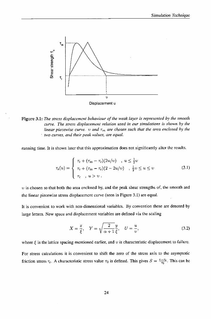
Simulation Technique
tm
0)
-c C) C ci
U)
CZ
-c Cl) Tr
1)
Displacement u
Figure 3.1: The stress displacement behaviour of the weak layer is represented by the smooth curve. The stress displacement relation used in our simulations is shown by the linear piecewise curve. v and Tm are chosen such that the area enclosed by the two curves, and their peak values, are equal.
running time. It is shown later that this approximation does not significantly alter the results.
Tr + (Tm - T)(2U/V) U <
T(U) Tr+(TmTr)(22U/V) , V<U<V (3.1)
Tr U>V.
v is chosen so that both the area enclosed by, and the peak shear strengths of, the smooth and
the linear piecewise stress displacement curve (seen in Figure 3.1) are equal.
It is convenient to work with non-dimensional variables. By convention these are denoted by
large letters. New space and displacement variables are defined via the scaling
X=., Y=/_2
, u= :?±, (3.2)
a+1 v
where is the lattice spacing mentioned earlier, and v is characteristic displacement to failure.
For stress calculations it is convenient to shift the zero of the stress axis to the asymptotic
friction stress Tr. A characteristic stress value r0 is defined. This gives S = This can be TO
24

Simulation Technique
written more explicitly using Equation 2.20.
32u 3u2 2v(a + 1)(d - d')G 2v(d - d')G (r - =
= (a + 1)2 + " S
_ 2v(d - d')C62 (3.3)
The reason for an extra factor of in the scaling Y as compared to X becomes apparent
here. It means that in terms of stress there is an equivalence between the X and Y directions.
A typical value of the Poisson ratio for a slab is 0.2 which gives an a value of about 0.3. Sites
will be approximately 1.2 times further apart across slope as compared to down slope.
Time is scaled according to
T=C1V[i t, (3.4)
where the non-dimensional parameter Ct defines the time step size.
Finally a non dimensional acceleration can then be defined as
A = C2a
(3.5) g sin 0
where a is the dimensional acceleration. The g sin 0 term is due to the fact that the interial mass
is p(d - d') while the shear stress is pg(d - d') sin 0.
Unless otherwise stated, the results will be presented in these non-dimensional variables.
32 Smbtrnll Technique
Each site is given two labels, i and j which represent its across and down slope position respec-
tively. All variables that are site specific (displacement, internal stress etc) are then given the
subscripts i and j which specify which site is being referred to.
Due to the discrete spacing the Laplacian of the displacement field (_5_X7 + is replaced by
the discrete second order gradient
St = + U_1 + U1 + U_1 - 4U , (3.6)
Therefore the stability equation (Equation 2.23) becomes
[U +1 + U_l + Ui +l + Ui_l - 4Ujj + Sext - Sij < 0 (3.7)
25

Simulation Technique
where Sext is the non dimensional external stress and S(U) is the non dimensional shear
stress supported by the site [ii]. If the stability relation is not fulfilled then this becomes a
discretised force balance equation, and the right hand side is replaced by a non dimensional
acceleration A 3 .
Initially the non-dimensional displacements U 3 and velocities Vij = AUij /Ct are zero for all
sites. For each time step the velocities are adjusted via
Vj + CA13 , >V,
vij -+ v, V2 + CtA ij < V, A 3 > 0, (3.8)
0,
Equation (3.8) allows the slab only to move into one direction (down slope), as only positive
velocities Vij are allowed. The use of a minimum value Vij can take (defined V) accelerates
calculations close to equilibrium configurations where a correct representation on the dynamics
is not important. V is chosen to be small enough so as to not affect the simulation results. The
same holds for the time step parameter C.
The displacement of each site is updated according to U -p Uj + CV3 . New strengths Sij
are computed, and the change in internal stress is evaluated. This process is repeated until a
static stable position is found, or large scale failure occurs.
The dynamics may be more complex than implied by Equation 3.8. However Middleton [36]
showed for a class of related models that, as long as the parameters V, C t and AS are chosen
to be small enough, the model will trend towards a unique pinned solution if the applied stress
is small enough such that the system possesses a stable configuration. Therefore even if the
behaviour of local instability and motion are significantly more complex than described above
the displacement profiles after ever stress increment will be the same. This implies that the
overal behaviuor would not be significantly affected.
It is clear that rupture within the slab will have a significant effect on the force balance equa-
tions. This effect is incorporated by defining the binary variables B'., and B. B is the mode
II rupture indicator; it quantifies the state of the bond between sites [i, i] and [i - 1, j]. Simi-
larly, the mode-I-indicator B indicates the state of the bond between sites [i, j] and [i, j - 1].
These indicators can take the values 0 or 1. B" = 1 meaning that the corresponding bond is I/IT
indicating . . . . intact and B, = 0 indicating that the bond has ruptured. Initially, the slab is assumed intact
Ell

Simulation Technique
(B" = 1 for all i, j). Rupture occurs if the corresponding stress between sites exceeds the 23
non-dimensional tensile/shear strength of the slab Sij The stress in the slab is proportional
to the relative displacement of adjacent sites. If rupture occurs then the corresponding rupture
indicator is set to zero:
0, - U_ 1,) -sJ , 0 , - U,_1) —S
BP 1, —SP < (U - U_ 1,) < S!, B' = 1, —S < (U - U,_1) <23 %3 1
0, - U_1,) > S , 0 , - U,1) ~ S 1.
(3.9)
If rupture occurs then this will affect the internal stresses. This is because stresses cannot be
directly transmitted across ruptures. The term for the internal stress (Equation 3.6) has to be
modified to account for this;
5lflt = B 1 (U +i - U) - B J (U - U_1)
+ ij+ I(Uij+l - U) - B(U - U_1) . (3.10) 23
The simulations are run by increasing the external stress from zero in small steps AS. This is
continued until any site becomes unstable (that is Equation 3.7 is violated). The displacement
of that site is increased by an amount Vii as calculated according to Equation 3.8. The new
internal stresses are computed, and it is checked whether all the sites are stable. If this is not
the case then the velocity of the unstable site(s) is(are) adjusted according to Equation 3.8 and
the process repeated until the velocity of all the sites is zero. If a stable position is found then
the stress is incremented again, and the process is repeated. If no stable configuration is found
then widespread basal failure will occur. The external stress at which this occurs is called the
critical stress and denoted S c .
As widespread basel failure progresses the stress within the slab increases because displacement
gradients build up. Rupture will then occur. The ruptured region will accelerate until the
simulation is ended. The simulations are ended when the maximum displacement exceeds a
threshold value Umax, which is chosen large enough such that the results do not depend on it
(in our simulations Umax = 100). Details about the various parameters are recorded throughout
the simulation.
Simple modifications can be made to the model to study other situations. Some sites can be
27

Simulation Technique
given very large peak strengths, so that they act like static objects (such as trees and rocks)
within the snowpack. A slope can deliberately have a flaw introduced to it, to simulate the
affect of a skiers tracks cutting the slope. This is done by setting the rupture strength of a line
of sites to either zero or a fraction of its original value.
709

MEMO ji Analytical Solutions and the Validatio
of the Computational mode.'~
In the previous chapter a cellular automaton computer model of slab avalanche release was dis-
cussed. There is one non-trivial situation where analytical solutions exist for the corresponding
continuum model, and this can be used to validate the simulations. This is a single shear band
in an otherwise homogeneous weak layer. The one dimensional case is considered first. Ana-
lytical solutions for critical stress and displacement profile of a stable shear band are derived,
and compared to the simulation results in Section 4.1. The behaviour of an unstable shear band,
and the associated rupture of the slab are considered in the following section (Section 4.2). The
simulations use a simple piecewise linear approximation to the stress displacement curve to
minimise computing time. In Section 4.3 the influence of this approximation on stability is
studied. Finally a two dimensional shear band is considered in Section 4.4.
4i Oinie Dllrnemlsioall Stabile Shear Baund
In this section a stable, one dimensional shear band is considered. A shear band is defined as an
extended area over which the strength of the weak layer has dropped to the residual frictional
value. The problem of displacement and failure due to a one dimensional shear band in an
otherwise homogeneous weak layer was originally solved by McClung in 1979 [17]. This
work built upon the classic paper of Palmer and Rice [16] on shear failure in over consolidated
clay slopes. McClung considered a shear band which is parallel to the shear force (y direction
in the coordinate system used here). This meant that the failure was in mode II. The shear band
considered here is in the x direction, perpendicular to the shear force. This means failure will
be in mode III. Without loss of generality, the shear band is centered at x = 0 and has width 21,
(see Figure 4.1). The maximum displacement, Um, will occur at x = 0.
29

21 Slab Weak Layer
X x=O
Figure 4.1: A one dimensional shear band of length 21, centred at x = 0, is considered. The strength within this region has dropped to it's residual frictional value Tr. There is a stress concentration at each end of the band. Beyond these the stress is equal to the external stress Text. The end region are defined as the regions where the external stress rises from Tr to a peak value and then drops back to Text.
41.1 Displacement lPrroiliuile
A critical or marginally stable shear band is defined as one where the failure and the resisting
forces exactly balance. Failure will occur if either the length of the band, or the external stress,
is increased infinitesimally. Assuming that the external stress Text is homogeneous then over
the entire length of the band the following equation will be satisfied
Iiii + Text - TS (U) = 0. (4.1)
By analogy, Equation 4.1 can be envisaged as describing the undamped motion of a particle
of mass Ijj in a potential V = f[Text - T(U)]dU. It follows that the solution must satisfy
the 'energy conservation' criterion V(no) = V(u m ) and hence uo and uma,, must fulfill the
relation [Umax
J (Text - Ts(U))dU = 0. (4.2) Uo
Let u, be defined as the displacement where the descending branch of the stress-displacement
30

Analytical Solutions and the Validation of the Computational Model
curve assumes the value r = Text (see Figure 4.2). To satisfy the Equation 4.2 then
,.u.
fUUx/[r(u) - Textldtt = [Tt - T(U)]dU . (4.3)
Ju0 .
A shear band with a maximum displacement of umax under an external stress of Text is consid-
ered. The stress displacement curve of the weak layer, with corresponding features of the shear
band marked, is seen in Figure 4.2. Graphically the first term in Equation 4.3 corresponds to
area I, and the second term to area II. For a critical shear band, area I will equal area U. For a
stable (non critical) shear band, area I will be larger than area II.
The end region is defined as the length over which the strength of the weak layer drops to the
residual value Tr (see Figure 4.1). Approximate analytical relations for a critical shear band can
be derived if the length of the shear band is large in comparison with that of the end region.
Within the band, away from the end regions U >> U 4 T Tr. Equation 4.1 can be
approximated by
Ijjj 49X2
= —(Text - Tr) . (4.4)
Differentiating once with respect to x gives
- (Text - Tr) + C1. (4.5)
ax - Iiii
However since the solution is symmetric around x = 0, and so the constant of integration, Ci,
must be equal to zero. Differentiating again gives
u(x)- (Text - Tr) 2
+ C2. (4.6) 21111 -
C2 can be evaluated by considering the condition that displacement at the edge of the band is
zero (l_±1 = 0). This implies C2 = Tc,_Tr12 The displacement profile is hence 21
(12 - X 2 )(Text - Tr) U (x) = 21111
(4.7)
Transforming into non-dimensional coordinates gives
(L 2 - (4.8) U(X)=
2
31

Analytical Solutions and the Validation of the Computational Model
tm
C) PD
Text cc CD
(I) T
-u
Displacement u
Figure 4.2: For a stable shear band area I will be larger than area H. For a critical (marginally stable) shear band area land area II will be equal. u, is defined as the point where the descending branch of the stress displacement curve equals the external stress.
The maximum displacement is found at X = 0,
Umax - L 2 SC
(4.9)
It is seen in Figure 4.3 that the results of the simulations show good agreement with the pre-
diction of Equation 4.8. The small difference is due to the approximation u 0 implicit in
Equation 4.4.
4.1.2 Stability Relation
The critical stress is the stress at which failure occurs. Analytical critical stress relations can
be derived if the shear band is long in comparison to the end regions. For a long shear band
the maximum displacement will be large in comparison to u* (um >> ut). This means that
T3 Tr. This means that f Umax
[Text - T(u)]du (area II in Figure 4.2) is approximately equal
to (Text - Tr)Umax. Substituting this into Equation 4.3 gives
- 1du (Text Tr)Um. (4.10)
We define the characteristic displacement by ü and Tm as peak shear strength.
f (T(u) - Tr )du (Tm - Tr)Ü (4.11)
32

Analytical Solutions and the Validation of the Computational Model
30
25
0 20
CU
10
C) (1)
-15 -10 -5 0 5 10 15
Scaled Position
Figure 4.3: The displacement curve of a critical shear band. The full line shows the simulation result while the dotted line is the analytical prediction (Equation 4.8). The half length of the band (L) was equal to 10 and the failure stress (S e) was equal to 0.5.
a, U,
a,
C,)
T
t r U
Displacement (u)
Figure 4.4: i is defined as a characteristic displacement. The areas enclosed by the curve and the step function are equal.
33

Analytical Solutions and the Validation of the Computational Model
119
LD 0.1 (I) ci)
U—
1 10 100
Scaled Shear Band Half Length (L)
Figure 4.5: Critical stress was found to be inversely proportional to the shear band half length. This rule broke down at low lengths due to edge effects. At higher lengths the models results were about 30% larger than the analytical predictions.
A graphical description is shown in Figure 4.4. Using Equations 4.7,4.10 and 4. 11, the approx-
1 imate relation (d - d') [l(Text - T 2 Tr))
= (m - T)ü. 4.12 4C (d—d')
is obtained. The term on the left hand side is an expression for the driving term which provides
the energy to drive the crack. The term on the right hand side is the resistance to shear band
extension [17].
The relation 4.12 has been previously derived from a quite different line of reasoning by Mc-
Clung for the case where shear failure is in mode II[17]. This leads to a slightly different
combination of elastic moduli on the left-hand side of Equation 4.12 (McClung obtains 2E
where as in mode II we would obtain 2(1 + c)E).
In non dimensional units this relation simplifies to
L 2 S Sm. (4.13)
A slight difference is found between the numerical and the analytical results. Figure 4.5 shows
the simulated and analytical critical stress values for shear bands of different lengths. As ex-
pected there is an inverse proportional relationship between shear band length (L) and critical
34

Analytical Solutions and the Validation of the Computational Model
stress (Se ). This relationship breaks down for short shear band lengths because the end zones
become large in relation to the shear band length. For longer shear bands the models results are
approximately 30% larger than the analytical ones.
41.3 Stability Relation via Griffith Energy Arguments
The stability relation (Equation 4.13) can also be calculated using a Griffith argument. Griffith
assumed that the crack (or in this case shear band) will start to grow in an unstable manner when
the total energy released by an infinitesimal increase in length becomes larger than the energy
needed to drive the crack that distance. In the case of a shear band, there are three different
forms of energy associated with the crack. Potential energy is released by the downhill motion
of the slab. Surface energy is needed to break bonds to create new surfaces and thus increase
crack length. Finally there is the elastic energy associated with the deformation of the slab.
Kinetic energy is not considered as the shear band approaches the critical point slowly. If
Etotai is defined as the total energy associated with the crack, and I as the half length of the
crack, then unstable propagation will occur when dEtpi <•dl
In this section it becomes convenient to work with non dimensional variables as the expressions
are more concise. Initially the potential energy term is considered. The energy released by a
unit of snow will be the external force (S t ) times the displacement of that region. The total
potential energy release will be the external stress times the displacement, integrated over the
length of the shear band (—L to L).
L Ep = Sext I UdX (4.14)
J—L
Solving this equation with the displacement profile (Equation 4.8) gives
p— 2SL3 —
(4.15)
The elastic energy stored in a material is given by Equation 2.18. In one dimension, and in
scaled variables this relation simplifies to
1 L E.
I-L ()2 dx (4.16)
2
35

Analytical Solutions and the Validation of the Computational Model
Again this can be solved by substituting in the displacement profile (Equation 4.8). This gives
an elastic energy of
E. = SL3 (4.17)
Finally there is the surface energy created due to the formation of the crack. This is defined as
E. The energy required drive the crack forward one site is equal to 0.58m. The length of the
crack is 2L. Therefore the surface energy associated with the crack is
E = LSm (4.18)
The total energy associated with the crack will be the sum of these three energy terms (Equa-
tions 4.15, 4.17 and 4.18). At low crack lengths energy must be expended to advance the crack.
In this case the crack will be stable. However at larger crack lengths more energy is released by
the growth of the crack than is needed for it to grow. In this case the crack is likely to propagate
in an unstable manner. There is a critical point between these two regimes when dEp1 = 0dL
(see Figure 4.6). This gives the relation
—2S 2 L 2 + Sm + SL 2 = 0. (4.19)
Rearranging gives
Sm = SL2
(4.20)
An energy of 2 Sm L (shown as Ebarr ier in Figure 4.6) has to be put into the system to get the
crack into this critical state.
Again it should be noted that Relation 4.20 is only applicable if the length of the shear band is
large in comparison to the end regions.
4.2 Ustabile Shear Band Behavmiir
In the previous section relations for a critical (marginally stable) shear band were developed. If
the length of, or stress acting on, such a shear band was to be increamented then the shear band
will become unstable and will start to grow. In this section we investigate the behaviour of an
unstable shear band in both an analytical manner and with our model. This can be used to test
how well the model work in a more dynamic regime As unstable shear band expansion occurs
me

Analytical Solutions and the Validation of the Computational Model
Energy released (Ep) Energy created (Ee+Es) Total Energy (ETO,)
Positive
Crack Length
Negative
Figure 4.6: The energy associated with the crack. At low crack length the energy released by the crack is less than the energy needed to drive the crack forward. There is a critical point ( dEjy]aI = 0) beyond which more energy is released by crack advancement than is needed to drive it, and the crack will propagate in an unstable manner
the stress in the slab at the edge of the band will increase. When this stress reaches a critical
value then rupture of the slab will occur. It is possible for events to occur the other way round,
for rupture to occur before widespread basal failure. However field observations and results of
this model suggest that this is not the usual sequence of events [3].
4,2.1 Uirristallie Expansion
In this section the behaviour of the shear band during unstable expansion, and the associated
rupture of the slab are investigated both analytically and numerically. A one dimensional shear
band which (in non dimensional units), has half length L and is centred at X = 0 is considered.
We assume that after failure the shear band maintains a parabolic displacement profile with
a curvature which, in general, will be different to that of a stable shear band (Equation 4.8).
The validity of this assumption will be demonstrated in the following. A numerical factor c is
introduced to account for the change in curvature. The displacement profile is
U(X)(L2 - X2)S = (4.21)
2c
For an unstable shear band the elastic forces at the edge of the band will resist the downward
motion of the slab. By considering the forces involved, a relationship between the curvature
37

Analytical Solutions and the Validation of the Computational Model
value c and the acceleration A of the slab can be calculated.
Initially a free sliding one dimensional band of snow of length L is considered. In this case an
external stress, magnitude 2SC L acts on the snow. The slab has a mass per unit area of sin 0
The sin 9 term disappears with the the scaling of acceleration (Equation 3.5). Therefore the ac-
celeration of the snow is equal to Cr2 , the non dimensional time parameter. The displacement
of the snow will be
U(T) = U(0) + C 2T 2 . (4.22)
It is shown later that the simulation results for this situation show good agreement with this
approximate analytical relationship.
For the case of the unstable shear band the total force will be reduced by the elastic forces
pulling upwards at the edge of the band. This elastic force will be the derivative of the displace-
ment profile. Differentiating Equation 4.21 and substituting X = +L, the force at each end
of the band is found to be Lsc. The band has two ends and so the total upward force will be
double this. The mass will still be sin 0
Summing the forces acting on the band, and dividing by the mass, (again the sin term drops out
due to the scaling) gives the acceleration of
A = c1 2 (i -
(4.23)
The values of A and c can be calculated using energy arguments. Firstly the kinetic energy of
the slab is considered. The standard expression for kinetic energy (mv 2 ) transforms in non
dimensional variables into
Ek = C2 SLV 2 . (4.24)
If constant acceleration is assumed and that the displacement of the band before failure is small
compared to max displacement then V 2 2AUmax . Substituting in the expression for Umax
(Equation 4.21 with X = 0) gives a kinetic energy of
Ek= L 3S,2 CA
(4.25) C
Substituting in Equation 4.23, the factors of Ct cancel out and this gives an expression for
38

Analytical Solutions and the Validation of the Computational Model
o Model points before Basel Failure
13 Model points after Basel Failure
12 Critical shear band profile
11 Unstable shear band profile
10 A A
-
130 0 10 1020 30
Postion (X)
Figure 4.7: The displacement profiles predicted by the model (data points) and the analytical solutions (lines) for a critical shear band, and a shear band just after basal failure. The profile very quickly changes from one regime to the other
kinetic energy just in terms of c
Ek= (L3S2) (_)
(4.26)
Slab avalanches only take a few seconds to release, and during this period the starting zone can
be thought of as a closed system. This means that the net change in energy is zero. An amount
of energy 2 (Sm ) 15 /S has to be put in to drive the system to the critical point (see Figure 4.6).
After that energy released by the system will be transformed into kinetic energy.
2)' Ep+Ee+Ek+Es
3S (4.27)
where L c is defined as the critical half length of the shear band. The elastic and potential
energy are calculated as for Equations 4.15 and 4.17, but using the displacement profile 4.21.
This gives the expressions
E - Sc an
L = 2SC L3
respectively. (4.28) d E
3c2 3c
The terms for elastic, potential and kinetic energy grow with P. The surface energy term E
39
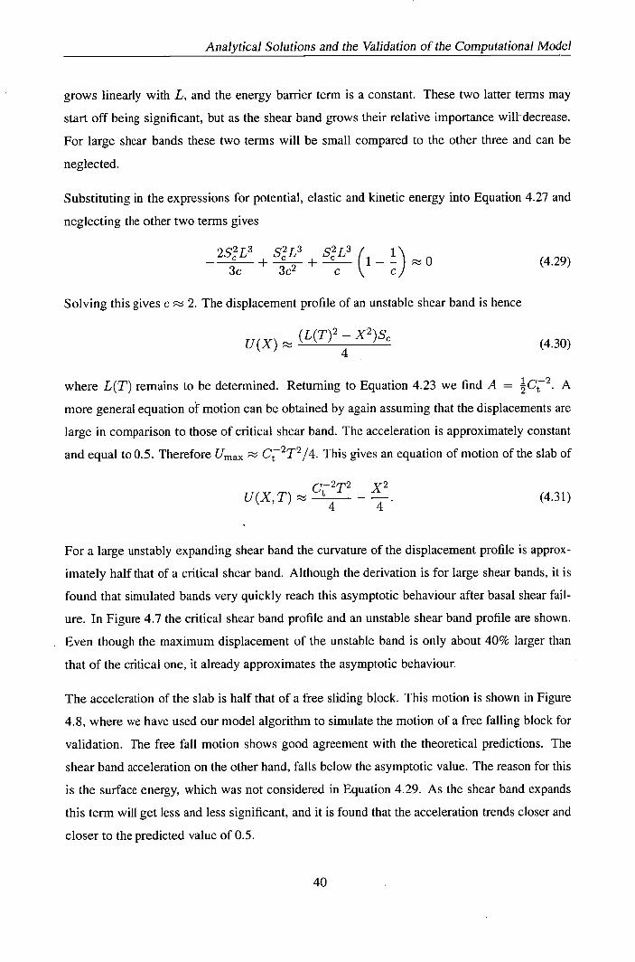
Analytical Solutions and the Validation of the Computational Model
grows linearly with L, and the energy barrier term is a constant. These two latter terms may
start off being significant, but as the shear band grows their relative importance will decrease.
For large shear bands these two terms will be small compared to the other three and can be
neglected.
Substituting in the expressions for potential, elastic and kinetic energy into Equation 4.27 and
neglecting the other two terms gives
2SL 3 SL 3 SL 3 + (1 - 0 (4.29)
- 3c 32 + c c)
Solving this gives c 2. The displacement profile of an unstable shear band is hence
(L(T)2 - X 2 )S (4.30) U(X)
4
where L(T) remains to be determined. Returning to Equation 4.23 we find A = A
more general equation of motion can be obtained by again assuming that the displacements are
large in comparison to those of critical shear band. The acceleration is approximately constant
and equal to 0.5. Therefore Umax C 2 T 2 /4. This gives an equation of motion of the slab of
C 2T2 U(X,T)
- •
(4.31)
4 4
For a large unstably expanding shear band the curvature of the displacement profile is approx-
imately half that of a critical shear band. Although the derivation is for large shear bands, it is
found that simulated bands very quickly reach this asymptotic behaviour after basal shear fail-
ure. In Figure 4.7 the critical shear band profile and an unstable shear band profile are shown.
Even though the maximum displacement of the unstable band is only about 40% larger than
that of the critical one, it already approximates the asymptotic behaviour.
The acceleration of the slab is half that of a free sliding block. This motion is shown in Figure
4.8, where we have used our model algorithm to simulate the motion of a free falling block for
validation. The free fall motion shows good agreement with the theoretical predictions. The
shear band acceleration on the other hand, falls below the asymptotic value. The reason for this
is the surface energy, which was not considered in Equation 4.29. As the shear band expands
this term will get less and less significant, and it is found that the acceleration trends closer and
closer to the predicted value of 0.5.
40

Analytical Solutions and the Validation of the Computational Model
300
E 250
200 E rl ca 150 a- C',
Free Fall Motion
100
50 Unstable Shear Band
Co
Theoretical predictions 0
0 200 400 600 800 1000 1200
Time Step (1)
Figure 4.8: The acceleration of an unstable shear band is predicted to be half of the free fall acceleration. Therefore the displacement will increase at half the rate of afree fall case. In this figure Ct = 10. In model the initial acceleration was less than this due to edge effects.
4.2.2 Rupture
In general rupture will occur after basal failure. In the case of a shear band the onset of rupture
can be estimated analytically. As the shear band expands the stresses in the slab increase. The
greatest tension will be found at the edge of the shear band ( X = ±L). The tension is equal to
the derivative of displacement (Equation 2.22). For an unstable shear band the maximum stress
will be therefore be Rupture will occur when this stress reaches a critical value (defined
S'/"). The half width at which this occurs is denoted L. Combining these gives
2S" Lr— ,
ext (4.32)
The model results show a linear increase in avalanche width (LO with rupture strength (see
Figure 4.9 left). However there is a discrepancy between the numerical and the analytical
results. This difference is caused by small scale stress oscillations arising from the numerical
integration algorithm (Figure 4.9 right). The numerical discretisation of space causes sequential
breaking of sites which creates "waves" in the displacement profile. The apparent tensile stress
will therefore reach the rupture strength sooner than otherwise expected. As a consequence, the
widths predicted numerically are approximately 40% less than those predicted analytically.
41

Postion (X)
Analytical Solutions and the Validation of the Computational Model
d60 / 0 .0
-195 so- / / o"
40- / //
o 30 / a'
/ Avalanche halt width vein 20 / - Avalanche half width
analytical notation 10
O'I -60%ot analytical solution
Rupture Criterion (R)
Figure 4.9: Left; The half width of the avalanche increased linearly with rupture strength, but these values were about 60% of those predicted analytically. Right; The tension in the slab approximatley increased as was expected. However waves resulting from the numerical discretisation caused the rupture strength to be met much earlier than expected.
43 Stress=Dispilacmeinit Curve anfluence
It was shown previously in the simple cases where analytical solutions exist they are approxi-
mately recovered by the model. These simulations use a linear piecewise approximation to the
stress displacement curve. In this section the resolution of the model is increased to study, in
detail, the edge of the shear band and the influence that different stiess-displacement curves
have on stability.
Three different stress displacement curves are studied; the typical hardening-softening curve
measured by McClung [18](called smooth), a linear piece wise curve assumed elsewhere in the
model (referred to as triangular curve in this section), and a simple box curve (see Figure 4.10).
The area under all the curves is same (equal to O.5S m ) and equal areas lie under the curves on
both sides of the point U=0.5. S m is defined as the peak strength of the triangular curve.
The resolution of the model was increased to resolve better the behaviour at the edge of the
shear band. The half width of the shear band used was 50, and S m was chosen as 0.05. This
value of Sm was chosen because the as the resolution increases (in this case by a factor of 10)
the corresponding peak shear strength reduce by a factor of the resolution squared (100 in this
case). This is explained in more detail in Section 5.3. Failure occured earliest in with simulation
which used smooth stress displacement curve. This gave a critical stress of 0.00368. The sim-
ulation with the box curve gave a critical stress of 0.0039 1, 6 percent stronger than the smooth
curve. Finally simulation using the triangular curve was the strongest with a critical stress of
42

Analytical Solutions and the Validation of the Computational Model
I Smooth stress-strain curve Triangular curve
1.00 A
Box curve
CO
Cn
I
0 1 2
Displacement (U)
Figure 4.10: Simulations were run using the three stress displacement curves shown above. All the curves enclose the same area (0.5Sm ), and with equal area to the right and the left of the displacement U = 0.5.
Smooth
Smooth
0) S 0
I0 0. od
to
(I, a Cd
Cd
Y
V
Figure 4.11: The displacement profile and tensile stress of shear bands using the three different stress displacement profiles. The critical stress was 6 and 11 percent larger for the box and triangular curves as compared to the smooth curve. This is the similar to the differences in tension and maximum displacement.
43

Smooth TrianuIarJ
Analytical Solutions and the Validation of the Computational Model
-
0.8 U)
0.6
(I, ci)
0.4
cci C
i5 0.2 C
- 0.0 (ci C.) U)
-0.2 -70
IN
Figure 4.12: The internal stress distribution were reminiscent of the corresponding stress dis- placement curves. The maximum internal stress was approximately equal to the peak shear stress of the corresponding curves minus external stress.
0.004 1, 11 percent larger than the smooth curve. These values are all slightly smaller than
the theoretical prediction (from Equation 4.13) of a failure stress of 0.0044. The differences
seen in displacement and stress within the slab are shown in Figure 4.11. These differences are
approximately proportional to the difference in critical stress. It is seen later that other factors
have a much stronger influence on critical stress and avalanche size.
The internal stress is different, there are large differences between the three examples (Figure
4.12). The shape of the internal stress curve is reminiscent of the shape of the associated stress
displacement curve. It can be expected that unstable expansion of the shear band will initiate
when the sum of the internal and external stresses exceeds the peak shear strength. Figure 4.12
shows the internal stresses at the last stable configuration of the shear band. As expected the
sum of the internal and external stresses are marginally smaller than the peak shear strength in
all cases. Therefore the height of the curve will correspond, up to a factor of the external stress,
to the peak internal stress.
ro-
As mentioned earlier the smooth curve is qualititively the same as has been measured [ 1 8].
However, computationally it is also the most complex. In all other simulations the triangular
curve is used. This is because it maintains displacement hardening softening behaviour pro-
-60 -60 -50 -40
MI-1.

Analytical Solutions and the Validation of the Computational Model
duces similar results to the smooth curve, while it's simplicity will reduce computer running
time.
44 Two Dimellhlsoilall Shear Bands
Displacement and stability relations were derived analytically for a one dimensional shear band.
The numerical results showed reasonable agreement with the analytical solutions. This proce-
dure is now repeated for the two dimensional case. The method used for deriving the analytical
results is similar to that in one dimension. These are then compared to the numerical values.
For a large critical shear band a generalisation of the force balance equation (Equation 4.4) is
IIH + IH - = (Yext - Tr). (4.33)
It becomes convenient to transform into non dimensional units at this point. This scales the
dimensions to be equivalent. Equations 4.33 becomes
a2u au + = Sext. (4.34)
Analytical solutions only exist for the simplest case; a circular shear band in an otherwise
homogeneous weak layer. Without loss of generality the shear band is assumed to be centred at
X = 0, Y = 0 and have radius L.
Due to the radial symmetry it is natural to use a polar coordinate system. R is defined as the
radial coordinate, and 4 as the directional coordinate. In this system 2j + 02u transforms toOY
1 (R9U) ± 1 92U As both the down and across slope coordinates have been scaled to be
equivalent, there can be no q5 dependence. This means that = 0. Equation 4.34 becomes
1 8 (4.35) / 8U\ (R) = Sext.
This is solved by integrating and applying boundary conditions, much in the same way that
Equation 4.4 was solved. In this case the boundary conditions are I R=11 = 0, and UIRL =
0. This gives
U(R)= (L 2 - R 2 )Sext
(4.36) 4
45

Analytical Solutions and the Validation of the Computational Model
300 Circular Shear Band I
250 Long Shear Band
E 200
CL 0 CII
150
E 100
E CO
50
0 5 10 15 20
Half Length of Shear Band
Figure 4.13: The maximum displacement of a two dimensional shear band at a given external stress was half ofthatfor the one dimensional case. In both cases the results fitted the theoretical predictions (Equation 4.8 and 4.36) well.
The simulation results show good agreement with the analytical solution (Figure 4.13). For
a given external stress and shear band size, the peak displacement is half of that for the one
dimensional case. This is not unexpected the elastic forces due to the extra dimension will
effectively double the resistance to displacement.
This extra dimension will also have an affect on the critical stress of the shear band. A similar
procedure is carried out as for the energy calculations in Section 4.1.3. The expression for the
potential energy is found to be
E =
7L4St (4.37)
The elastic energy is irL4 S t
(4.38) Ee= 16
and finally the surface energy is irL2 Sm
E = 2
(4.39)
46

Analytical Solutions and the Validation of the Computational Model
0.1
o Circluar shear band, model results r'.irrIiiar hpar hand, theoretical values
17 Cl)
U) U, ci,
U)
Cs ()
1 10
Shear Band Radius (L)
Figure 4.14: As in one dimension the critical stress was inversely proportional to the shear band size. This was not the case for small shear bands due, to edge effects.
Differentiating these terms, and summing them to zero gives the relation
L' S2 4Sm. (4.40)
The models results and the analytical solution are shown in Figure 4.14. Unlike the one di-
mensional case, the numerical predictions are slightly smaller than the analytical solution. The
numerical results flatten off for small shear band sizes where the end zones become significant.
In two dimensions the displacement profile of a circular shear band of radius L will be half
that found in one dimension. It is expected (and found numerically) that after failure the shear
band profile will continue to be one half of it's one dimensional equivalent. Differentiating the
displacement profile means that the maximum stress in the slab will be 0.25SextL. Assuming
that rupture will occur when LUL equals the rupture strength S", the avalanche will have a dR
radius (L) of 4S"
L = . (4.41) 8ext
This will give an avalanche area A of approximately
A -- 167r(S'1")2
(4.42) (Sext ) 2
47

Analytical Solutions and the Validation of the Computational Model
The area of an avalanche will hence be proportional to the square of the tensile strength of the
snow. Due to the shear band spreading out in a circular manner through a square grid, sites
at the edge of the band will fail progressively rather than simultaneously as occurred in one
dimension. Therefore the "waves" seen in one dimension due to the numerical discretisation of
space, do not occur in this case. Rupture occurs very close to the value suggested by Equation
4.41.
45 C©llndllus©llns
Avalanche release is essentially a fracture mechanical problem, and only in the simplest cases
do analytical solutions exist. Any numerical models should approximate the analytical solu-
tions for these cases. Initially a one dimensional shear band was considered. Relations for the
displacement and critical stress of the shear band were derived. The displacement profile com-
pared favourably with the analytical solution. An unstable shear band is found to accelerate at
approximately half the rate of a free sliding block. Rupture occurs when the stress within the
slab reaches a critical value. In the simulations rupture occurred earlier than predicted by the
analytical solution. This was because numerical oscillations caused by the space discretisation
in the edge of the shear band caused the rupture strength to be exceeded earlier than expected.
The influence of different stress displacement curves was considered. The results calculated
using a realistic (called smooth) curve were compared to those using piecewise approximations.
All gave similar results. A piecewise triangular curve is assumed throughout the rest of this
thesis. This is because it produces similar results, and its simplicity reduces computing time as
compared to the smooth curve.
Finally a two dimensional shear band was considered. Again the simulation results agreed with
the theoretical expectations.
48

am =111-0
As discussed in the Introduction, large random variations in weak layer shear strength are an
almost generic feature of avalanche prone slopes. Initially (Section 5.1) the nature of weak
layer variability, and the way in which it can be incorporated into the model, are considered.
The effect of this variability on slope stability is investigated in some detail in Section 5.2.
In Section 5.3 the resolution of the model, and the correlation length of the randomness are
considered. It is found that increasing the resolution does not affect critical stress. This means
that the coarse discretisation used elsewhere in this model is sufficient. The correlation length of
the randomness does however have a strong knock down effect on slab stability. Snow is known
to be a time dependent material, and the influence of the time healing of damaged regions is
considered in the following Section (5.4). The significant effect of variability, and lack of effect
of time healing suggests that internal stresses play a critical role in the failure process. This is
explored in Section 5.5. The existence and effect of so called "hotspots", areas which are more
prone to avalanche initiation, are studied in Section 5.6.
The final two sections focus on avalanche size. Initially the size of a single avalanche (Sections
5.7) is considered. Then the size distribution of many avalanches (Sections 5.8) is investigated
and compared to field observations.
51 Mode Parameters
Here we use the same model as was tested against the analytical solutions in the previous
chapter. However the shear strength of the weak layer is allowed to vary randomly in space
rather than show well defined areas of shear failure such as described in the previous chapter.
A second source of randomness can be introduced by allowing for variations within the rupture
strength of the slab.
49

Model Results
SiLl Shear Strengths
Unless specified otherwise all sites are given random independent peak shear strength values
Sm , the subscript m indicating maximum site shear strength. The distribution of the strengths is
characterised by two values; (S,,,) denotes the mean, and a the variance of the shear strengths.
A Weibull distribution is used, as this is the often the distribution associated with strengths.
However this does not seem to be an important assumption as the results remain almost the
same for a box distribution. The Weibull distribution has the cumulative distribution function
P(Sm ) = 1— exp [—(Sm1g),3] . (5.1)
The distribution is characterised by the Weibull parameters S and 3. These relate to mean and
relative variance via (Sm) = sr(i + 113) and a' I(SM)2 = F(1 + 2/13)/[F(1 + 17/3)]2 - 1,
where F denotes the Gamma function. The relative variance is the square of the coefficient of
variation.
5.1.2 Rupture Criterion
Although variations in the rupture strength of the slab are less documented than weak layer
shear strength variations, it is likely that they will exist. This second source of variability can
be introduced by allowing the rupture strength to vary in a similar way to the weak layer shear
strength.
We considered two situations. In the first the basal shear strength was allowed to vary randomly
while the rupture strength S" is kept constant. This is called the homogeneous slab case.
In the other case rupture strengths of the slab were randomly and independently drawn from a
Weibull distribution in the same way as the basal shear strengths. This meant that both the weak
layer and slab strengths had the same relative variance. This is called the non homogeneous
slab case.
5.1.3 Parameters Used
To correctly simulate an avalanche release, the parameters used in the model have to be non
dimensional versions of those found on real snow slopes. Typical dimensional values are stated
in Appendix A. In the following we used, unless otherwise noted, the following set of 'standard

Model Results
0 EiJ 87.50 -- 100.0
El 75.00 -- 87.50
10 Eli 62.50 -- 75.00 L J50.00 -- 62.50
37.50 -- 50.00
20 25.00 -- 37.50 12.50 -- 25.00 0 - 12.50
>- 30
40
50 0 10 20 30 40 50
x
Figure 5.1: The displacement profile at the end of one simulation. A cohesive area of slab (marked as gray) has avalanched. The crown and side walls of the avalanche are clearly marked by the thick black lines. The positive y direction is associated with down slope. A simulation size of 50 by 50 sites is chosen here for clarity.
weak layer parameters': (S m) = 5 and (o, 2 , I(SM)2) = 1. This level of variability is at the
upper end of what has been reported from field tests. The discretisation of the individual sites
was chosen as the length scale of the randomness, so that the strengths can be treated as inde-
pendent random variables. It is shown later that increasing the spatial resolution (more sites per
correlation length) does not affect the results.
The tensile strength of the slab has been reported to be two to four times larger than the shear
strength of the weak layer [37]. A factor of 2 is assumed, which gives a non-dimensional
rupture strength of (S") = 10.
In general a system size of 100 x 100 sites was used as this is big enough to be statistically
representative of a large slope but still requires short running times.
Boundary conditions were imposed by giving sites on the edges of the simulation very large
shear strength (ST = 1000). This means no avalanche activity occurs on the edge of the
simulation. The stress and displacement increments AS and V were chosen small enough such
that the final results did not depend on them, but large enough that simulation running time
was not a major issue. For typical parameters, this was fulfilled for AS and V < 0.1; in the
simulations the values AS = V = 0.01 were used unless otherwise noted. The simulations
51

Model Results
1.4
1.2
S1.0 CO
0.8
0.6
0.4
0.2
0.0 I ... , II I
0 2 4 6 8 10 12 14 16 18 20 22
Slab rupture strength (S u" )
Figure 5.2: Critical stress was not affected by slab rupture strength. Simulations details (Sm) = 5, (0.2 = 1, simulation size 100 by 100 sites with data point averaged over 30 simulations. As with all the figures in this chapter, error bars represent plus and minus one standard deviation.
were run until the maximum site displacement reached a critical value, usually 100. By this
time an area of the slab has clearly avalanched (Figure 5.1).
Two other situations were studied by varying specific site parameters. Specific sites could be
given very large shear strengths so they act like static objects (such as trees and rocks) within
the snowpack. In the other case the slab deliberately had a flaw introduced to it, to simulate the
effect of a skiers tracks cutting the snow. This was done by setting the rupture strength of one
row or column of sites to either zero or a fraction of its original value.
5,2 Slope Stabiity
Variations in weak layer shear strength were found to have a profound effect on slope stability.
This effect and other phenomena caused by basal shear strength variability are considered in
this section. It was found that slab strength (51111) had little influence on critical stress (see
Figure 5.2). All the results in this section (unless specifically mentioned otherwise) assume
that the slab is homogeneous and S 11II = 10.
52

Model Results
1E-4-4-- 1.2 1.4 1.6 1.8
Failure stress S.
a 1.8
a 1.6 °D.
1.4 0 0
1.2
0
0.2
0
0.1 0 0 0 0000 0 0 0
0.0 0 40 80 120 160 200
99.999
CL 95 >
70 . 40 0
CL 10 U)
1 (Ti
U- 0.01
U) (0 U)
U)
(Ti 0
Ti
A
A
ci? V
V
Simulation size
Figure 5.3: Main Figure; The probability distribution of slope failure stresses determined for
an ensemble of 600 statistically similar simulations. ((Sm) = 5, (o/(Sm ) 2 ) = 1
and a size of 100 by 100 sites). The solid line shows the result expected for a Gaussian distribution which is in good agreement with the simulation results. Top Right; The decrease of critical stress with slope size. Bottom Right; The decrease in variance of critical stress with increasing slope size. In both these figures (Sm) = 5, (01(Sm ) 2 ) = 1 with the simulations size varied as indicated.
5.21 Critical Stress
Since we assumed the randomness of the site strengths, the critical stress for a particular sim-
ulation was itself a random variable. For a large ensemble of statistically similar simulations
the critical stress was approximately Gaussian distributed (see Figure 5.3). Statistically similar
meaning the statistics (mean shear strength, relative variance of shear strength, simulation size
etc) were the same for each simulation.
The average critical stress dropped off with increasing slope size (Figure 5.3, top right). This is
plausible as large systems have an increased probability of containing very weak configurations,
which will fail at lower stresses. However this size effect was quite weak compared with other
effects considered later. The variance also dropped off with slope size (Figure 5.3, bottom
right). Again this is quite plausible as larger slopes are likely to be statistically more similar
than small slopes. This implies that, at least in our model smaller slopes are on average more
stable but less predictable than larger slopes.
The average critical stress increased in an almost linear manner with average peak strength
(Figure 5.4, left). A very significant result is the rapid drop off in critical stress with relative
variance (Figure 5.4, right). Even a very narrow strength distribution can have a dramatic effect
on slope stability. This suggests that localised weak configurations have a strong influence on
53

6
5
(I)
0, a,
Ca
:2 0
Model Results
5 10 15 20
Average cell strength <S,,>
I o Homogenous Tensile 4.0 Rupture Strength
I o Non Homogenous Tensile 3.5 ,
A I Rupture Strength
2.5
In 2.0
1.5 n 0
§io
0.0 0.0 0.2 0.4 0.6 0.8 1.0 1.2 1.4 1.6
Relative variance
(.2j<%>)
Figure 5.4: Left; The dependence of critical stress on average site strength (S m ) is almost linear Simulation size 100 by 100 sites with (o. i /(Sm ) 2 ) = 1. Each data point averaged over 30 simulations. Right; The dependence of slope failure strength on weak layer variance. Weak layer shear strength (Sm ) = 5. For open symbols both weak layer and slab rupture have a relative variance indicated on x axis. The closed symbols indicate the slab is homogeneous. The simulation size 100 by 100 sites, each data point averaged over 30 simulations.
the failure process.
As mentioned before, in general rupture strength had little effect on the critical stress. This was
not the case for the non homogeneous slab at very high variabilities. In this case sites which
happened to have both weak shear strengths and rupture strength failed individually at very low
stresses. In this case the snow was more akin to powder than slab, and the results were similar
to small powder snow sluffs.
An analytical formula can be fitted to the results to give an approximate relation between the
critical stress, the average shear stress of the weak layer and the relative variance (see Figure
5.5. This is
(Sc ) 0.28 (Sm) (0-1 /(Sm ) 2 ) °45 . (5.2)
This formula is not very accurate for very narrow shear strength distributions as the formula
diverges for o —* 0 while the simulations results converge to S m . There has been no attempt
to introduce the effects of slope size into this relation because of the weak effect that it has. A
more complex formula could be derived that did not diverge for o, 2 = 0 and took account of
slope size effects. This has not been as this formula was derived to make qualitative comments
about the effects of variance.
54

Model Results
H 'N •1 0
o <S >=2
3X <Sm>=5 Np
o <Sm>=10 C3 Box distribution
,- Sc=0.28<Sm>(CT2/<Z.)m>
2)
-0.45
I..I
0.1 1
Relative variance ( 2/<Sm>2)
Figure 5.5: Scaled critical stress (defined as Sc / (Sm )) versus relative variance. The models results compared to Equation 5.2. The simulation results are for (Sm) = 2 (cir-
cles), 5 (stars) and 10 (open boxes). The closed boxes correspond to simulations whereby S' were selected from a box distribution. Simulation size 100 by 100 sites, each data point the average of 10 simulations
A E
C/) V
C/) (J) 'I) ci, C,)
0
C.)
a) Cci 0
U)
10
2.1
2.0
-Th 1.9 CI)
1.8 C,)
1.7 U)
1.6 0
1.5 0
1.4
1.3
0 10 20 30 40 50
Distance between static objects
Figure 5.6: The influence of static objects on slope stability. Simulations parameters; (Sm) 5, (o 1 /(S"' )) = 1, 100 by 100 sites, with each data point averaged over 10 simulations.
55

50
40
30
> 20
10
0 0 10 20 30 40 50
x 1 10
Distance (R)
0 C 0
C.) C
IL C 0
0.1 1)
0 0
Model Results
The effects that static objects as such rocks have on slope stability were then considered. In
Figure 5.6 the effect that a network of rocks of different distances apart has on critical stress
is seen. Rocks had a significant stabilizing effect if they were less than about ten sites apart.
Further apart than this, they made little difference to critical stress. In general the avalanches
only occurred between rocks, meaning a typical avalanche size will be less than in the absence
of static objects.
Figure 5.7: Left; A typical damage pattern just before failure. The black squares represent the failed sites (Uij > 1). A simulation size of 50 by 50 sites was used for presentation purposes. Other simulation parameters used were (Sm) = 5 and (o i /(Sm ) 2 ) = 1. Right, The correlation function C(R) against R. This shows a power law decay C(R) x up until a characteristic length of R 18. After this point C(R) is independent of R. This graph was made from an ensemble of 20 simulations with (S m ) = 5,(0 i /(Sm ) 2 ) = 1 and size of 100 by 100 sites.
5.22 Damage Patterns
Information about the failure mechanism can be inferred by studying the displacement pattern
of a slope just before failure. To quantify this, a damage function was defined as unity for a
failed site (Uij > 1) and zero otherwise. We considered the damage correlation function C(R),
which is the probability of finding a second failed site a distance R from any given failed site.
This function is defined as C(R) = where i12 + j'2 = R 2 . The function was
evaluated over all values of R and, to improve the statistics, this process was repeated for an
ensemble of many systems (in this case about 20 systems). The damage function just before
failure for a typical slope, and the correlation function as averaged over many slopes are shown
in Figure 5.7. Up to a characteristic damage correlation length (R e ) of about 18, a power law
Zvi

Model Results
decay C(R) oc Rm, with rn 0.8 was observed. Above this C(R) was independent of R.
This implies that over the limited length scale 1 < R < R, the damage distribution could be
described as a random fractal set with dimension D = 2 - m = 1.2. Above this there was a
cross over to a Poisson random pattern with fractal dimension 2. Investigation of the damage
function for different simulations sizes confirmed that the correlation length Rc did not depend
on system size. In these simulations periodic boundary conditions were applied to prevent edge
effects.
5
.0
0.
0,
(I)
3.0
PW
2.0
1.5 .0
0. 1.0
'0 0.5
0 0.0 0.5 1.0 1.5
External Stress (Sm ) 0.0 65 1.40 1.45
External Stress (Sm)
Figure 5.8: Left; Precursor events recorded during one simulation. Two types of precursor can be seen, creep and bursts. Simulation parameters; stress increment AS = 0.001,
Sc = 1.44, (S m ) = 5, (0 i /(Sm ) 2 ) = 1, 100 by 100 sites. Right; A more detailed view of the section leading to failure.
5.2.3 Precursor Events
Due to the random variations in the weak layer, local failure occurs before global failure. This
can be investigated by studying the displacement changes which occur after each stress incre-
ment. Susceptibility was defined as the total change of displacement per unit external stress
increment. Figure 5.8 shows the susceptibility for a simulation with stress increment step size
(AS) of 0.001. Two distinct types of precursor events were seen. Firstly there was a kind of
creep activity, where the susceptibility slowly and steadily increased with stress. Then there are
large but short lived (usually just one stress increment long) increases in displacement. These
are concentrated towards failure. These bursts generally correspond to two or more sites failing
at one time.
In a real system, these displacement increments may be detectable through acoustic emissions.
Acoustic activity has been reported to be greater in unstable snowpacks than in stable ones
57

Model Results
[38] [39]. Despite these results were inconclusive two types of signal were identified: type I
spikes and type II continuous noise. It is thought that the former signals may originate from
macroscopic cracks and the latter from differential movement on the shearing surface. If these
emmisions were from the snowpack then match well with the behaviour observed with the
model.
53 ResoRufion and C©rreilatli©llhI ILeinigtllui
The results discussed in the previous section were produced using a spacing equal to the corre-
lation length of the basal shear strength variations. In this section the results of increasing the
resolution of the model to check whether using a finer grid size affects slope stability. As the
correlation length of the randomness is a physical quantity, the number of independent strengths
values on the slope does not vary with resolution. Therefore resolution could be increased by
keeping the number of independent strength values on a slope constant, while increasing the
number of sites. The strength values for the additional sites could be calculated by interpola-
tion. A slope size of 12 by 12 correlation lengths was chosen. This gave one hundred and forty
four random, independent peak shear strengths. These were calculated in the usual manner.
The resolution is defined as the number of sites over which the shear strength varies randomly,
and is designated by the letter N. N was restricted to the integer values 1,2,3,4,6,8,10 and
12. For a resolution of one (N = 1), there were exactly the same number of sites as random
strengths. Sites were directly given the random strengths and the basic version of the model was
recovered. However for N> 1, random strengths were assigned to a fraction 1/N 2 of the sites,
located on a grid of spacing N, and the strength of the other sites were interpolated from these
values. There are many different ways in which the interpolation could be carried out. The
simplest method is linear interpolation. This was not chosen as it leads to a non-differentiable
strength field and alters the strength statistics from the initially assumed Weibull distribution.
A cosine squared function was derived and used instead. This was because the derivative of the
strength field was continuous and the statistics were not significantly altered (Figure 5.9).
At a resolution of N, the sites [i = aN], [j = bN], where a and b are equal to integers,
were assigned independent values. The peak shear strengths of the other sites on the column
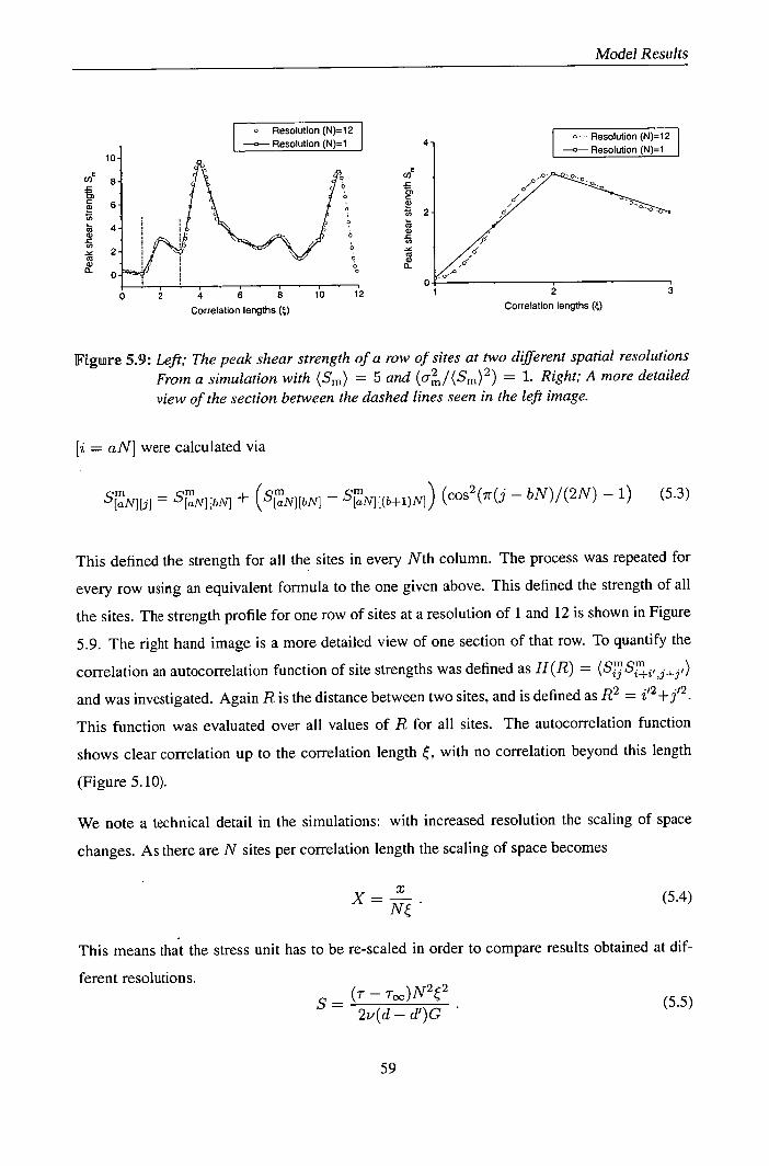
E
0) C a,
CO
Ca a, 0)
(a (1) 0
- Resolution (N)=12 Resolution (N)=1
0) C VD ZS 2 Ca a) CO
a, a, 0.
Model Results
r ' Resolution (N)=12 Pnh,tinn IN\1
0 2 4 6 8 10 12
Correlation lengths () Correlation lengths ()
Figure 5.9: Left; The peak shear strength of a row of sites at two different spatial resolutions From a simulation with (S m) = 5 and (o/(Sm ) 2 ) = 1. Right; A more detailed n. view of the section between the dashed lines seen in the left image.
[i = aN] were calculated via
SN][] = SN][bN] + (SM N][bN] [aN][(b+1)Nj) (cos2((j - bN)1(2N) - 1) (5.3)
This defined the strength for all the sites in every Nth column. The process was repeated for
every row using an equivalent formula to the one given above. This defined the strength of all
the sites. The strength profile for one row of sites at a resolution of 1 and 12 is shown in Figure
5.9. The right hand image is a more detailed view of one section of that row. To quantify the
correlation an autocorrelation function of site strengths was defined as H(R) =
and was investigated. Again R is the distance between two sites, and is defined as R 2 = i'2 +j'2 .
This function was evaluated over all values of R for all sites. The autocorrelation function
shows clear correlation up to the correlation length , with no correlation beyond this length
(Figure 5.10).
We note a technical detail in the simulations: with increased resolution the scaling of space
changes. As there are N sites per correlation length the scaling of space becomes
x XN (5.4)
This means that the stress unit has to be re-scaled in order to compare results obtained at dif -
ferent resolutions.
- - (r - r)N2e2
(5.5) 2v(d—d')G
59

Model Results
45- 000 0 N=12'
0 I o N=4 40
00 I I
0 t C Do
35 00
Do
30 0•
i 800800000000000000000c
0 0 0 0 0 0 U
25
20 2 3
Correlation lengths ()
Figure 5.10: The auto correlation function H(R) shows correlation up to the correlation length scale . results for resolutions of N = 4 and N = 12 are shown. Simula-tion parameters; (Sm ) = 5 and (o i /(Sm ) 2 ) = 1. Data points averaged over 20 simulations.
A non dimensional unit of stress increases with N 2 , meaning that the peak shear strength of the
sites scales with 11N 2 . After all the sites have been defined with the interpolation technique
described previously, their strength was divided by N 2 to account for the different stress scaling.
This make sense intuitively; if the dimensions of a site are reduced by a factor N, then their
area will be reduced by N 2 , and so the strength will also be reduced by this factor.
In the following we compare simulations of slopes with different spatial resolution and rescale
all stresses to standard (N = 1) units.
Increasing the resolution in this manner did not significantly affect the critical stress (Figure
5.11). It is also seen that the relative variance of the distribution of site strengths did not vary
significantly with correlation length (Figure 5.11).
This interpolation technique could also be used to investigate the effect of correlation length on
slope stability. In this scheme, the number of sites per simulation was kept constant, and there
was no re-scaling of the stress units. This meant that N corresponded to the correlation length,
rather than the resolution. Again we allowed N to take the values 1,2,3,4,6,8,10 and 12. For
each of these correlation lengths, twenty simulations were run to improve the statistics. It was
found (Figure 5.12) that increasing correlation length has a strong knock down effect on slope
stability. This is expected because for large correlation lengths, areas around weak sites will
readily form large shear bands. These will result in failure at low stresses.
ME

C 2.0
V o - 1.5
1.0 Cu V
Cu
' 0.5
0.01 0 2 4 6 8 10 12
Resolution (N)
'A 1.2 U) V
0.8 C Cu
Cu >
0.4
Cu
Cr 0.0
0 4 8 12
Resolution (N)
Model Results
Figure 5.11: Left; The effect of increasing resolution on critical stress (when stress is scaled back to standard (N = 1) stress units) Right, The effect of the cos 2 interpolation technique on the relative variance the weak layer shear strengths. For both figures (Sm) = 5, (0- 2 I(S.)2) = 1, simulation size 100 by 100 sites, and the results averaged over 20 simulations.
54 Effect of Shear Streigh Recovery
The model assumes that the weak layer loses shear strength as the bonds are broken by the
displacement of the overlaying slab. Any motion or slippage in the snow can be considered
to be instantaneous in comparison to the external stress increment timescale. However, snow
is a time dependent material [9], and the possibility that strength increases due to sintering
processes should be considered. It was assumed that the rate at which strength increases will be
proportional to the number of broken bonds that are available to sinter, and this in turn will be
proportional to the drop in shear strength. The strength increase per time step (L.'r) is therefore
proportional to the difference between the peak strength Tm and the present strength r of that
site,
T=cO(Tm T). (5.6)
In the absence of other factors, a damaged region would asymtopically regain its initial strength.
However, at the same time as the bonds are healing, the external stress is increasing meaning
that there is competition between healing and damaging processes. The relative rates of these
two processes is expressed by , the ratio of the sintering timescale (T8 ) to the external stress
increment timescale Text. W can take values between 0 and 1. W = 0 would represent an
infinite healing time, and the non time dependent model would be recovered. = 1 would
imply immediate recovery (in comparison to the external stress increment timescale) of any
61

2 4 6 8 10 12
Correlation length (N)
0.0 0
2.2 A
co 2.0
1.8 Cn
1.6
1.4
1.2
5 1.0
cc 0.8
0.6
0.4
0.2
Model Results
Figure 5.12: Varying correlation length while keeping all other variables constant has a strong knock down effect on slab stability. Simulation parameters (S m) = 5, (0,2 I(S",)2) = 1, simulation size 100 by 100 sites with each data point being averaged over 10 simulations.
damaged areas.
The implementation of the time dependent model was essentially the same as for the standard
model. The difference was that, prior to each stress increment, every site which was damaged
(defined by Ujj > 0.5) but stable (Vj = 0) would increase in strength. The strength increased
by a factor ISij = p(S - S') where SJ was a site's peak shear strength. The external stress
was then incremented again and the process repeated until failure.
It was found that time healing of damaged sites has little effect on the critical stress (see Figure
5.13). In simulations with > 0.2, the critical stress is more or less independent of W, and
these values are only about 15 per cent above the W = 0 values. Time healing also had little
effect on damage patterns and precursor events.
It has been argued by Louchet that the increase in the strength of the weak layer will be pro-
portional to the number of broken bonds squared [10]. He argues that two broken bonds are
necessary for the welding reaction. This is the case in many types of diffusion or transport con-
trolled chemical reactions. If this were the case, then the strength of a damaged region would
grow at a different rate than in our simulations. This argument is, however, dubious as bonds
neither diffuse nor are transported. However given the limited effect that time healing had in
general, the details of strength growth are likely to have little effect on the critical stress.
62

Model Results
1.01
1.00
(ID -c 0.99
Cn
0.98
C')
CZ 0.97 a)
Cl) 0.96
1.5
C,)
1.0
C,
0.5 0
0.95+ 0 40 80 120 160 200
time T
0.0 0.00 015 0.50 0.75 1.00
Time scale ratio p
Figure 5.13: Left; An example of the strength fluctuations of a weak site in the time dependent model ( = 0.1). Right; The change in critical stress with different p values. Simulation parameters (Sm ) = 5, (O 1 /(Sm ) 2 ) = 1 simulation size 100 by 100 sites. The data points in the right figure are averaged over 50 simulations. As with the other figures the error bars show plus and minus one standard deviation.
55 RnteirnaR Stresses
Time healing had little effect on critical stress. This implies that time healing did not largely
affect the main triggering process. After a site is displaces beyond U j = 0.5 then its strength
would decrease. However this strength could recover making it more resilient to the stresses
which act upon it. However its position could not recover, meaning that the internal stresses
acting upon it remained unchanged. This suggests that, at least in our model, internal stresses
played a significant role in the failure process.
When a weak site displaces it is likely that negative internal stresses would act upon it. These
would counteract the external stress, and the site would be supported. The stress was redis-
tributed to the surrounding sites causing them to experience positive internal stresses. In this
way internal stresses redistribute external stresses, but globally do not change the total shear
force acting on the slope. Close to failure complex internal stress patterns built up. Large areas
of negative internal stress (shear bands) were supported by a few highly stressed sites. In Figure
5.14 the development of the internal stress pattern in a slope at four different external stresses
is shown. The size of the simulation used was 30 by 30 sites as this shows the patterns clearly.
The first image (a) shows the internal stress pattern when the external stress was 58% of the
failure stress. Isolated pockets of low negative internal stress are seen. These correspond to
where weak individual sites have slipped. Often the corresponding positive internal stresses
row
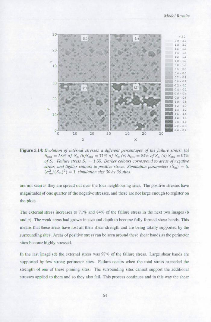
-.. + (a).
.. $-
4 .,
+
4 _4
4
*
10 20 30
X
30
20
10
30
20
10
0 0 10 20 30
X
Model Results
>22
2.0- 22
1.8- 2.0
1.6- 1.8
14 - 1.6
12- 14
1.0- 12
Os - 1.0
0.6- 0.8
0.4-0.6
02- 04
0.0- 02 r 402 - 0.0
14 --02
-0.6--0A
$1 -1 .0 -0.8
-12- -1.0
-14 --12
-1.6 --1.4
1S--1.6
-2.0 --1B
2 --2.0
-24 --22
Figure 5.14: Evolution of internal stresses a different percentages of the failure stress; (a) Sext = 58% of S,, (b)Sext = 71% of Sc, (c) S ext = 84% of S c, (d) Sext = 97% of S. Failure stress S 1.55. Darker colours correspond to areas of negative stress, and lighter colours to positive stress. Simulation parameters (Sm ) = 5, (0,2 /(S 111 ) 2 ) 1, simulation size 30 by 30 sites.
are not seen as they are spread out over the four neighbouring sites. The positive stresses have
magnitudes of one quarter of the negative stresses, and these are not large enough to register on
the plots.
The external stress increases to 71% and 84% of the failure stress in the next two images (b
and c). The weak areas had grown in size and depth to become fully formed shear bands. This
means that these areas have lost all their shear strength and are being totally supported by the
surrounding sites. Areas of positive stress can be seen around these shear bands as the perimeter
sites become highly stressed.
In the last image (d) the external stress was 97% of the failure stress. Large shear bands are
supported by few strong perimeter sites. Failure occurs when the total stress exceeded the
strength of one of these pinning sites. The surrounding sites cannot support the additional
stresses applied to them and so they also fail. This process continues and in this way the shear
64

Model Results
band spreads out in an unstable manner to cause widespread basal failure. This occured at an
external stress of 1.55 units.
In our model the processes leading to natural slab avalanche release can be summarised as fol-
lows: Local weak configurations encourage the growth of shear bands at low external stresses.
With increasing external stress these grow in small steps or jumps as sites or small areas fail.
These local failures produce the bursts seen as precursor events. The perimeters of these failed
regions become highly stressed. When another site fails, the shear band spreads out in an un-
stable manner. When the tension at the edge of the band reaches a critical value, rupture of the
slab will occur.
The larger the shear band the higher the stress on the perimeter. There is a quite well defined
maximum size which a shear band can grow to and still be stable. Beyond this size the perimeter
sites are unlikely to be strong enough to support the shear band, and it will expand in an unstable
manner to cause slope failure. For our standard parameters the largest stable shear bands are
approximately 17 to 20 sites in diameter. This is the largest distance whereby one site can
influence another before widespread failure occurs. Above this length scale it is expected that
there will be no correlation between sites. This would explain the turnover (around 18 sites)
observed in the correlation function (Figure 5.7).
This scenario explains why time healing does not greatly increase slab stability. Slope failure
is not directly caused by weak sites (which may go through many failure-recovery cycles).
Rather the creep of weak sites builds up internal stresses on the strong "anchoring" sites. Time
healing cannot reduce the stresses acting on these sites. This is because displacement and the
associated internal stress do not heal. When one of these sites fails, it is likely the shear band
that it supports will spread out quasi-instantaneously and large scale slope failure will then
occur. Time healing does not affect this quasi-instantaneously failure. This is because the
timescale for unstable shear band expansion is always much smaller than the time healing and
external stress increment timescale.
Finally internal stresses explain in a qualitative manner the strong knock down effect that vari-
ability has on critical stress. When there is no variability (o = 0), all the sites have the same
shear strength. Therefore they respond to external stress in the same way, meaning that no in-
ternal stresses develop and the failure stress is the same as the average shear strength. However
as the relative variance increases, the difference in the way that different sites respond to the
65

Model Results
external stress increases and so the internal stresses increase, which promotes earlier failure.
With increasing variance the critical stress decreases to a fraction of the average site strength.
56 99Hotspts9 '
As discussed previously, random weak layer shear strength variations seem to be a feature of
avalanche prone slopes. It seems likely then, that some regions of a slope will be more prone
to avalanche initiation than others. These areas where avalanche initiation is more likely are
termed "hotspots". Hotspots are observed when a skier releases a well tracked slope by being
unfortunate enough to hit such a weak region. The existence and influence of these hotspots
can be investigated using our numerical model. A slope was "primed" by applying an external
stress of 1.3 units to the slope which had a critical stress of 1.46 units. This corresponds to
89% of the critical stress. A simulation size of 30 by 30 sites was chosen for clarity. The
displacement profile of this primed slope is shown in Figure 5.15.
The main features of the displacement profile are four or five shear bands which are 2 or 3
sites wide. A skier descending the slope is assumed to cause local damage to the weak layer,
but not to significantly alter the total shear stress acting on the weak layer. Local damage was
simulated by setting the shear strength of an individual site to zero. If this did not cause the
failure of the primed slope, then the external stress was incremented until failure occurred. The
critical stress of the slope could be used as a measure of how much the local damage affected
global stability. The three possible outcomes were:
• the slope failed when the site was damaged.
• the slope did not fail when the site was damaged, but did fail at less than the critical stress
of the undamaged slope.
• the damaged slope failed at the same (or even higher) stress as the undamaged slope.
After failure the slope was "reset" to it's primed state (Figure 5.15), and the process repeated
for the next site. This allowed a "map" of the effect of individual site failure on global stability
to be built up (Figure 5.16). Hotspots can clearly be seen in this figure.
The main feature of this figure is a large cluster of hotspots in the top right hand side, and
a smaller group in the middle bottom of the figure. Generally these hotspots are associated
ATO
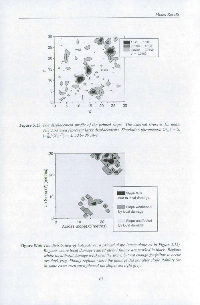
Model Results
30
0 . —1 125 -- 1.500
25 07500 -- 1.125
__ • 0.3750 -- 0.7500 0 - 0.3750
20
> 15 e;O
10 c
'D
5. c c, <'
0 0 5 10 15 20 25
KII
x
Figure 5.15: The displacement profile of the primed slope. The external stress is 1.3 units. The dark area represent large displacements. Simulation parameters; (Sm ) = 5, (al1 /(S m ) 2 ) = 1, 30 by 30 sites.
Ce
N'
20- a) E
>-a) .2 10
CDL
Across Slope (X)(metres)
Slope fails due to local damage
Slope weakened by local damage
Slope unaffected by local damage
Figure 5.16: The distribution of hotspots on a primed slope (same slope as in Figure 5.15). Regions where local damage caused global failure are marked in black. Regions where local basal damage weakened the slope, but not enough for ftiilure to occur are dark grey. Finally regions where the damage did not alter slope stability (or
in some cases even strengthened the slope) are light grey.
67

Model Results
3500
3000
2500
2000 Ca
1500
co
C
1000
500
0 — JrL
0 2 4 6 8 10 12 14 16 18 20 22
Rupture Strength (5Ca)
100
(a a) CO a) .c 10 C-, C ca (a
Homogenous Slab
1 0 Non Homogenous Slab
0
0.0 • 0.2 • 0.4 • 0.6 • 0.8 • 1.0 1.2 • 1.4 • 1.6
Relative Variance (02,,I<S>2)
0 = DO
D = = 0
o 0 0
o 0 0
0 0
0
Figure 5.17: Left; For the non homogeneous slab at a relative variance of one, the avalanche
sizes were approximately 40 percent smaller than if the slab were homogeneous. The solid line shows the theoretical results (Equation 4.41). Simulation parame-
ters; (Sm) = 5 and (O/(Sm ) 2 ) = 1. A simulation size of 200 by 200 sites was
used so that the avalanche area was not affected by simulation size. Error bars represent plus and minus one standard deviation. Right; Variability within the weak layer had a weak effect on the avalanche size. However variability within the slab had a strong knock down effect on avalanche size. Simulation parame-
ters; (Sm ) = 5, (S'/") = 10, size of 100 by 100 sites.
with shear bands. However there does not seem to be a hotspot between the two central shear
bands. This implies the location of weak spots depends on more than just the distribution
of shear bands. Hotspots are a natural result of strength variability and the associated stress
redistribution. Avalanches can be released well below the natural critical stress by localised
damage of specific regions of the slope.
5,7 AvaRanche Se
As well as slope stability, avalanche size was an important aspect of the overall avalanche
hazard. A relation between avalanche area and rupture strength for a uniform slab and weak
layer was derived in Chapter 4 (Equation 4.41 and 4.42). These relations predict that, for a
given critical stress, release area is proportional to the square of the rupture strength of the slab.
This was confirmed with our simulations (see Figure 5.17, left).
If the slab is homogeneous, then avalanche area is not strongly influenced by the relative vari-
ability of the weak layer (Figure 5.17, right). This is due to two competing factors which
approximately canceled out. The stress in the slab is approximately proportional the product

Model Results
400-
350 1 3.04
300.1 (00 J A A 2
n A
2501 A (0 2.5- N J A I
200I A I .c I 2.0-1
150-1 I CO I o No Notch Present I I
C.) I
100 A Notch Present 1 .5 1
o No Notch Present A Notch Present
0
0
80
0 0
1.01.
00 02 0.4 0.6 0.8 10 1.2 14 16 0.0 0.2 0.4 0.6 0.8 1.0 1.2 1.4 1.6
Relative variance (a2/<S,>2) Relative variance (a2/<S>2)
Figure 5.18: Left graph; The effect of notches on avalanche area. Right graph; The effect of notches on critical stress. In both case (Sm ) = 5, with a simulation size of 100 by 100 sites. Data points averaged over 30 simulations.
of the external stress and the radius of the shear band. Rupture occurred when this reaches a
critical value. High variability encourages rupture to occur at lower external stresses (Relation
5.2). Therefore the corresponding shear band radius has to be larger for rupture to occur. On
the other hand weak layer variability promotes stress concentrations which encourages rupture
sooner than predicted by Relation 4.42. These two factors approximately cancel out. Also
shown in this graph are the results for the non homogeneous slab. In this simulation The rela-
tive variance slab strength was the same as the weak layer shear strength. In this case variability
had a very strong knock down effect on avalanche size. At high variability individual weak sites
failed causing something that could be interpreted more as a powder snow sluff rather than a
slab avalanche.
The effects on slope stability and avalanche size of damage or cracks within the slab rather
than in the weak layer was considered. This was simulated by setting the rupture strength of
a band of sites to zero. Although a real ski track would show a more complex path than this,
the qualitative results are expected to be the same. It was found that even cutting the slope
completely in either the x or y directions did not alter the critical stress, and had little effect on
avalanche size (Figure 5.18). A notch stops the expansion of a shear band, but plays little or no
part in the process of shear band formation. This supports the idea that rupture is a secondary
process, only happening after widespread basal failure has occurred. It should be emphasised
that although the cutting of the slab by a skier seems unlikely to affect stability, damage to the
weak layer, which is also likely to occur, can have a strong knock down effect on stability (see

Model Results
A
a-MWIN
CZ 0 a-
0.01
E E o 1E-3
0.1 1 10
Slab depth (d-d)
Figure 5.19: Shown are 1000 data points drawn from the distribution P(d - d') = (d - d') -0-38
- 1. We use this is approximate the exceedence probability distribu-tion observed for real slab depths of P( ~! (d - d')) o (d - d') 26 (shown by the solid line) for (d - d') > 0.5, with a flattening of the curve below this value.
Section 5.6).
5 Avallallhldilhie Sfle DstHbuil©ini
The size distribution of avalanches can be used both for hazard evaluation, by for example
predicting the return period of particularly large avalanches, and for an insight into avalanche
release processes. Various authors report that both natural and triggered avalanches [40], [23],
[24], in common with other geophysical phenomena such as landslides, show a power law size
distribution [23]. This means that the probability that an avalanche will be of area A or larger is
P(> A) oc A, where ,8 is the power law coefficient. The cumulative probability distribution
P(> A) oc A—
1-2 has been recorded for nearly 4000 blast triggered avalanches [40] [23].
This corresponds to a non cumulative probability distribution of P(A) x
Our model was used to investigate the size distribution of the avalanches. Initially this was
done for a large ensemble of statistically similar simulations for both homogeneous and non-
homogeneous slabs. In both cases the avalanche sizes showed a Weibull distribution. However
it was discovered that if inertia was neglected, a very small step size (LS = V = 0.001)
70

Model Results
14 D DDQ
A
0.1
cj .0 0
a- 0.01
lu
10 100 1000 10000
Avalanche Area (A)
Figure 5.20: The exceedence size distribution of avalanche area for an ensemble of 240 simu-lations. The solid line shows power law function P( ~: A) oc A —
1 - 2 reported for
a large ensemble of slab avalanches.
were used and the slab was non homogeneous, then the avalanche sizes showed a power law
distribution.
This power law in the absence of inertia was also found by Faillettaz et. al [23]. They believe
the power law distribution to be due to some form of critical phenomena. However as seen
in real sandpiles, these critical phenomena only emerge in the absence of inertia. As inertia is
important in real avalanches then Self organised criticality or other forms of critical phenomena
are unlikely to be the cause of the observed power law distribution. Another possible cause for
the power law size distribution is the distribution of controlling parameters. McClung analysed
data on 187 fallen dry slab avalanches [24]. His results show a power law distribution of crown
wall heights (d - d' in Figure 2.1) for heights greater than 0.5 metres. For heights less than this
value the distribution flattens out. The power law coefficient was 2.6. Other sources quote a
similar distribution of slab depth [ 23], [40].
McClung also reports that average weak layer shear strength increases with overlaying slab
depth to the power 1.22 [24]. This is because at greater slab depths, greater normal forces will
encourage greater bonding across the weak layer. This effect was incorporated into the model
by assigning each simulated slope a "slab depth". This value was uniform for all the sites in one
simulation. The shear strength for individual sites was calculated in the usual manner and then
71

Model Results
multiplied by the slab depth to the power of 1.22. This simulation was run until slope failure. A
new slab depth was calculated and the process repeated. A large ensemble of simulations were
run assuming the distribution of slab depths found by McClung (Figure 5.19).
In the case when the slab was non homogeneous an approximate power law size distribution
was found (Figure 5.20) over about two orders of magnitude. The slope of this power law
showed a complex dependence on the ratio of rupture strength to average peak shear strength,
the variance of these two quantities and stress increment step size used. The nature of this
dependence was not explicitly investigated. In general a power law coefficient of around 1 was
found, not dissimilar to the value of 1.2 reported in the literature.
This power law size distribution was not found for the case of the homogeneous slab. It seems
that two sources of randomness were necessary.
However the situation is complicated by the fact that mountain landscapes are generally fractal
in nature, with a dimension somewhere between 2 and 3 [41]. This would imply that terrain
features such as slopes and gullys show a power law size distribution. Avalanche sizes are often
controlled by the terrain features they occur in. Therefore size distribution slab avalanches
observed in the field may be a result of the size distribution of terrain features.
It seems clear that the power law distribution produced by the present model is not an outcome
of the collective dynamics inherent of the model (without further tweaking, a Weibull-type size
distribution is found). Rather it is 'inherited' from the power law distribution of slab depths
used as an input. The dynamics described by the model acts as a nonlinear filter which converts
one power-law distribution into another. In this sense these simulations support McClungs idea
that the power law distribution of slab avalanche sizes is not the signature of some kind of self-
organized critical dynamics or other critical phenomenon [24]. Rather it reflects the power-law
distribution of the governing parameters, and the relationships between these parameters.
53 Conchsk
In this chapter randomness was introduced into the model and the influence it has on stability
studied. All sites were assigned random independent Weibull distributed peak shear strengths.
The variance of this randomness, had a dramatic knock down effect on slope stability. Slope
stability was not affected by the rupture strength of the slab.
72

Model Results
In our simulations we used a relative variance of one, similar to that found experimentally by
Conway and Abrahamson. However, this value is significantly larger than that reported more
recently by various authors. If a smaller variance were assumed, then the knock down effect
of variability on stability would be less significant. However the internal stress patterns which
develop and lead to failure are not significantly different.
The derivation of the stress redistribution factor in Chapter 2 assumes the correlation length
scale of the randomness to be larger than the depth of the slab. Of course it is entirely possible
that the slab depth is equal to, or larger than the correlation length. If this were the case then
longer-range stress redistribution than is assumed in our model could occur. This will redis-
tribute stress over a larger area, reducing the intense local build up of stress on individual sites.
This will have a similar effect on the internal stress patterns as reducing the variability would
have. This would promote greater stability than our model would suggest.
We also make the assumption that the correlation length scale of the randomness is of the order
of one metre. A larger correlation length is likely to further reduce stability. This is because the
likely size of any deficit zone or shear band will be larger. The corresponding external stress
necessary to cause widespread failure will be smaller. Another assumption that we make the
shape of the stress displacement response of the weak layer. However as shown in Chapter 4,
this has little influence critical stress or avalanche size.
Although all the assumptions described above are likely to have an influence on the critical
stress of a slope, they are unlikely to affect the general processes (described below) that lead to
avalanche release.
Snow is a time dependent material. This was modeled by allowing damaged regions to regain
strength over time. This strength recovery had little effect on critical stress. Global failure is
preceded by precursor events, which may be detectable by acoustic emissions. These precursor
events come in the form of short bursts superimposed on a background 'creep' activity. Similar
acoustic emissions have been experimentally recorded in the snowpack close to an avalanche
prone slope. However these experimental results are not conclusive.
Internal stresses play a crucial role in the failure process. An investigation of the internal
stresses close to failure show patterns of large deficit areas being supported by a few key an-
choring points. These anchoring points correspond to strong, but highly stressed, sites. Slope
failure is triggered by the overloading of one of these anchoring points. An investigation into
73

Model Results
the slope damage patterns found correlations up to a length of about 18 sites. This is a similar
size to the largest shear bands which form before failure. So called "hotspots", areas where lo-
cal failure causes global failure at stresses well below the global failure threshold, are a natural
result of variability and the associated stress patterns that emerge.
All this suggests that natural slab avalanches release via the collective action of localized flaws
which leads to the nucleation of a shear band. These then grow in an unstable manner. These
processes are independent of the rupture strength of the slab. The shear band continues to
expand until the stresses at the periphery of the band exceeds the rupture strength of the slab.
At this point the slab ruptures and the avalanche accelerates down the hill. In reality this may
be an overly simplistic view. It is likely that changes is topography, snow properties and slab
depth will influence when failure will occur.
In our model avalanche dimensions are approximately proportional to the rupture strength of
the slab. Slab variability is found to reduce avalanche size. A reduction in area of approxi-
mately 40% is seen for a relative variance of 1. For a large ensemble of statistically similar
slopes a Weibull distribution of avalanche sizes was found. However power law distributions
of avalanches size could be obtained by introducing a power law like distribution of slab depths
and allowing the rupture strength of the slab to vary randomly. This supports McClungs asser-
tion that the power law distributions in slab avalanches reflect power-law distributions of the
governing parameters rather than some form of critical phenomona.
74

a I I =11 11
Traditionally snow stability evaluation has focused on weak layer shear strength. However,
as discussed in the Introduction, slab avalanche release is essentially a fracture mechanical
process. This means that the governing material property for avalanche release will be weak
layer fracture toughness rather than shear strength. There are three modes in which a crack
can be loaded; two of these (modes II and III) are in shear, and one (mode I) is in tension (see
Figure 6.1). The fracture toughness of the snow is likely to be different in each of these modes.
All three of these values are of relevance to slab avalanche release.
Fracture toughness was first predicted to be of relevance to avalanche release in 1979 [17].
However it was not until 1999 that the fracture toughness of snow was measured experimentally.
Initially research focused on measuring the mode I fracture toughness of homogeneous snow
using cantilever beam experiments [11] [12]. Values between about 0.1 and 1.5 kPa m 112 were
obtained depending on the snow type and density. However there has been some concern that
size effects in these measurements make the direct application of the results to large scale slab
avalanche models dubious [5]. More recently Kirchner et al. investigated mode II fracture
toughness, and the influence of friction on fracture toughness [42] [43]. Sigrist et al. [5]
consider the effect that specimen size and shape can have on fracture toughness measurements,
and derived a correction factor to account for these effects.
Here we report on an experimental program designed to measure the fracture toughness of
snow in all three modes. Initially the principles of linear elastic fracture mechanics (LEFM) are
considered (Section 6.1). In the next section both the experimental and the analytical techniques
used to measure fracture toughness are discussed (Section 6.2). We analyse the results taking
the findings of Sigrist et al. [5] [44] into account. The results are reported in Section 6.3. In
the final sections the effects of layering (Section 6.4) and friction (Section 6.5) are investigated.
Both were found to influence the results.
75

Fracture Toughness
Model Modell Made In
Figure 6.1: The three different modes offracture.
6.1 Lhear Elistflc Fracture Mechanics
Here we consider a special case of linear elastic fracture mechanics (LEFM), the Griffith crack.
Around any crack tip a local, non linear zone forms due to the stress concentrations found there.
LEFM assumes this region to be small relative to the crack length. The Griffith crack makes
the additional assumption that the material dimensions are significantly larger than the crack
length, meaning that edge effects can be neglected. The Griffith relation for the stability of a
crack in a linear elastic material is derived by considering the energy changes associated with
the growth of a crack.
We consider a one dimensional crack loaded in tension (mode I). There are three energies
related to the crack which we refer to as; surface energy, potential energy and elastic energy
[45]. The surface energy is the energy required to create the new surfaces associated with the
crack. This will be E = 2'ya where a is the half length of the crack, and 'y is fracture energy of
the snow, i.e. the required to form a surface of unit area. Energy is released by the displacement
associated with the crack. As energy is released via material displacement in a stress field, then
it can be considered a form of potential energy. This is found to be E = - a2a2, where
o- is the stress in the system and E is the Young's modulus of the material [45]. This value
is negative because the energy is released. However the elastic energy associated with this
displacement profile is Ee =2,a2 Therefore the total energy that is actually released by the
formation of the crack is ET = - ____
76

Fracture Toughness
2a
Figure 6.2: Linear elastic fracture mechanics considers a crack of length 2a which is under a uniform stress cr and is significantly larger than the non elastic zones found at the crack tips.
For small crack lengths the energy required to advance the crack will be larger than the energy
released by its advance (aET/aa > 0). At large crack lengths more energy is released than
is required to advance the crack (aET/aa < 0). The cross over between these two regimes
occurs when MT/,9a = 0. The value of a when this occurs is called the critical crack half
length and denoted a. Differentiating the expression for the total energy, and equating this to
zero gives cr2 7ra
= 2,y. (6.1) E
If a crack were to reach the critical half length, then more energy is released by the growth of
the crack is more than is needed to advance the crack. The crack will expand in an unstable
manner. By multiplying both sides by the Young's modulus (E), all the parameters which are
material properties are grouped together on the right hand side of this equation. The square root
of this combination is defined as the fracture toughness of the material
Kj (6.2)
Substituting this into Equation 6.1 gives the usual Griffith relation
KI C = u/W. (6.3)
77

Fracture Toughness
A similar expression is found in shear
Kj11jjj (6.4)
where r is the shear stress.
6.2 Experfleiitali Tethnque
The experimental method of measuring fracture toughness experimentally involves loading pre-
cracked specimens of standard geometry until failure occurs. If the fractures are macroscop-
ically brittle then the fracture load can be used to calculate toughness using a set of standard
tables for the compliance of the specimen. Most work focuses on measuring the mode one
fracture toughness. Mode one is concentrated on because generally it is the easiest to measure
experimentally. The experimental geometry often used is the three point bending of notched
beams.
For snow mode one fracture toughness has generally been measured by the cutting of cantilever
beams. This technique involves carefully harvesting a beam of snow from the natural snowpack.
The beam is held horizontally and carefully cut from the top until it snaps under its own weight.
By measuring the mass of snow which has broken off, and the depth of the cut when failure
occurs, the mode I fracture toughness can be calculated. We refer to this technique as the pure
cantilever technique.
In our test specially designed boxes which restricted failure to specific modes were used were
used. Weights could be placed on, or suspended from the apparatus to increase the stress within
the sample. A piece of string with a diameter of a few millimeters was used to saw through
the snow beam until failure occurred. String was used so that when cutting the block the crack
sides did not touch, thus eliminating friction between the crack faces.
These experiments were undertaken in the SLF cold laboratories at the Weissfiuhjoch field
station, near Davos, Switzerland during the winter of 2004/05. The use of the cold laboratory
allowed a constant temperature to be maintained for all the tests, thus removing any possible
temperature effects from the results. The cold lab also provided a calm and stable environment
to work in. Samples were collected from the natural snowpack around the Weissfiuhjoch using
a short section of square metal pipe of the same dimensions as the test devices. The snow

Fracture Toughness
beams were then transported into the cold laboratory where they were stored in sealed plastic
boxes at least overnight, but not more than two days, before they were tested. This allowed the
samples to settle to the laboratory temperature of -10'C but probably was not long enough for
significant changes to the snow properties to occur.
Snow is a highly variable, and often a rapidly changing material. To maintain consistency be-
tween experiments only a specific type of snow was harvested and tested. With the exception
of the experiments which focused on the toughness of a weak layer, all the experiments were
carried out on homogeneous snow consisting of small rounded particles with a density of be-
tween 250 kgm 3 and 350 kgm 3 and a hardness of pencil to one finger on the snow hardness
index. (The snow hardness index is a qualatitive measure of the hardness of snow developed
by field workers based on what object can be easily inserted into the snow. It ranges from fist
to knife. See [46] for more details.) The snow used for each set of experiments was given a
label between I and VI. Details of each snow type are given in Appendix B. To account for the
slightly different properties of the snow used for the different experiments, mode I measure-
ments were taken for snow types I, II, IV and V. There was at most a 12% difference between
these values. By scaling our results by the ratio of the mode I values, we attempted to eliminate
any differences in the results due to the different snow properties.
The fracture toughness of snow was first measured by Kirchner et al. [11]. They analysed their
data using a version of Equation 6.3 with a specific to their geometry. However Equation 6.3
is derived assuming the crack to be totally embedded in the material and the non linear zone
at the crack tip to be small relative to the crack length. When analysing our data we take the
findings of Sigrist et al. [51 into consideration. We use relations developed by Tada et al. [47] to
analyse our results. These relations give expressions for the critical stress intensity factor KQ.
Kirchner etal. [11] and Faillettaz et al. [12] equate this to fracture toughness K. However this
is only true if LEFM is valid.
For a beam geometry the size criterion for LEFM to be valid is [13]
a,p> 2.5 0.45 < a/h <0.55 (6.5) O's J
where p is the beam width, a is cut depth at failure and a 8 is the tensile strength of the material.
For snow of a density of 200 kgm 3 the ratio of toughness to strength is about 0.4 m 112 ,
meaning that the minimum sample size is approximately 1 metre [13]. The size requirement
79

J
Boxes full of snow a Cut down
h with wire
Jw V ____ Weight
Figure 6.3: Mode I device; Snow was carefully inserted into two hinged box sections. One section was attached to the table, and a weight was hung off the second section a
distance Jw from the hinge. The snow in the gap between the box sections was cut until failure occurred.
for the valid application of LEFM is unrealistically large for the harvesting of homogeneous
snow samples and for laboratory testing.
However fracture toughness can be related to critical stress intensity by [5]
K=/i+(9J)KQ (6.6)
where D is the sample size and D0 a characteristic size associated with the point when fracture
toughness rather than strength controls the failure stress. By fracturing samples of different
sizes in mode I, Sigrist et al. found that D0 0.33 m. Our tests were carried out on very similar
snow to that Sigrist used to calculate D0 . Therefore we assume that D0 is approximately the
same for our samples. Our sample size is fixed at D = 0.14 m. This means that
Kj 1.8KJQ (6.7)
For a first approximation we assume that this relation also holds in shear. The results of the
experiments are generally quoted in terms of critical stress intensities. However at the end of
each section the corresponding fracture toughness values are mentioned.

I
Fracture Toughness
Figure 6.4: The mode I experiment. Left; Cutting through the snow block at the gap between the box sections with a wire. Right; The device and fracture surface after failure. Although not apparent in this image, the fracture surface is rough, easily distin-guishable from the surface caused by the cutting with the wire.
6.2.1 Mode I
The mode I fracture toughness was investigated first as the experimental technique was the
simplest, and our technique was similar to that previous researchers had used. The device used
for these measurements consisted of two short sections of square metal pipe joined by a hinge
at the bottom (see Figures 6.3 and 6.4). One section was fixed to a table and the other projected
into space. The two sections were held together and a snow beam slid in. A weight was hung
from the protruding section a horizontal distance J from the hinge. A thin wire with a diameter
of less than one millimetre was used to cut vertically down through the snow beam at the gap
between the boxes, until failure occurred . As with all our experiments, the cutting was carried
out quickly to cause brittle failure and avoid ductile effects. Wire was used for this experiment
as the gap between the box sections was not wide enough to allow the string to pass through.
As failure was in tension, there was no friction between crack faces, and so cutting with a wire
instead of string did not alter the results. This was confirmed experimentally. We refer to this
method as the hinged cantilever technique.
This technique had some advantages over the pure cantilever technique described earlier. Due
to the presence of the hinge, the failure had no mode II component, and large weights (up to
10 kg) could be suspended from the protruding box section. This meant much larger tensile
stresses than could be produced than would be possible using body forces (the weight of the
cantilever) alone. This meant that measurements could be taken over a much wider range of
N.

Fracture Toughness
F s y
1>
Figure 6.5: The Tada relation we quote was developed for a three point bending test. Our situation is essentially an upside down three point bending test.
relative cut depths.
We use an analysis technique originally proposed by Tada et al. [47], which was used by used by
Sigrist [5] to analyse three point bending of a pre cracked beam. The situation that this relation
is derived for is shown in Figure 6.5.
KIQ=FI 2 s/ (6.8)
where F is the force acting on the beam, s the horizontal distance where the force is applied
and the support points, w the specimen width, h the specimen height and a the cut depth. The
function F1 is
F1 = 1.122 - 1.4 (~ ) + 7.33 (a)2 - 13.08 ( a )3
+ 14 ()4.
(6.9)
As with the other Tada relations that we we use, this is derived for shallow cracks (a/h < 0.6).
Due to the presence of the hinge in our device, our situation is equivalent to an up-side-down
three point bending test where F = 2Mw with M being the moment per specimen width.
82
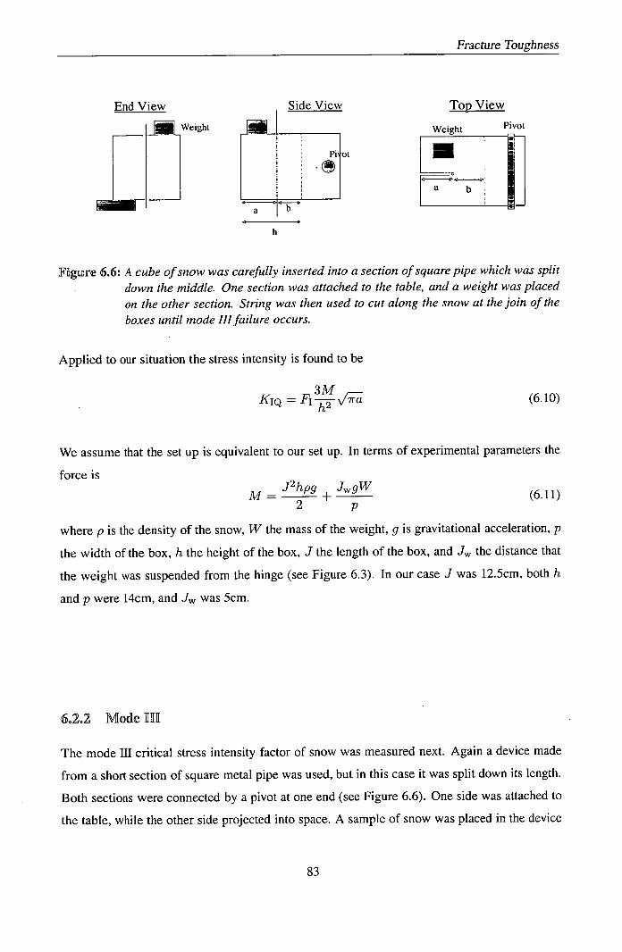
Fracture Toughness
End View
Weight
Side View Top View
Weight Pivot
LF b
h
Figure 6.6: A cube of snow was carefully inserted into a section of square pipe which was split down the middle. One section was attached to the table, and a weight was placed on the other section. String was then used to cut along the snow at the join of the
boxes until mode III failure occurs.
Applied to our situation the stress intensity is found to be
KIQ = Fj/
(6.10)
We assume that the set up is equivalent to our set up. In terms of experimental parameters the
force is
M = J2hpg + JgW
(6.11) 2 p
where p is the density of the snow, W the mass of the weight, g is gravitational acceleration, p
the width of the box, Ii the height of the box, J the length of the box, and Jw the distance that
the weight was suspended from the hinge (see Figure 6.3). In our case J was 12.5cm, both h
and p were 14cm, and Jw was 5cm.
6.22 Mode HE
The mode III critical stress intensity factor of snow was measured next. Again a device made
from a short section of square metal pipe was used, but in this case it was split down its length.
Both sections were connected by a pivot at one end (see Figure 6.6). One side was attached to
the table, while the other side projected into space. A sample of snow was placed in the device

Fracture Toughness
Figure 6.7: The nioc/e /1/ experiment. Left; Cutting through the snow block with a the string. In this picture the weak layer is being tested. The snow block had to be trimmed so that the weak layer coincided with the cutting plane. In the homogeneous tests the snow sample would fit better into the test device. Right; The device immediately after failure.
Figure 6.8: The fracture surface associated with mode Ill failure. The vertical groove was added after to distinguish the cut from the fractured area.
E:1

Figure 6.9: The Mode II! Tada relation for a crack beam with a shear force r acting parallel to the crack front (into the page).
and weights of up to 13 kg were placed on the projecting section. String was then used to saw
along the length of the beam, towards the pivot, until failure occurred (see Figures 6.7 and 6.8).
In mode III the relationship used for the analysis of the data was.
ira KIJJQ rFjjj,/F where F111 = tan . (6.12) ~ 7ra
where i- is the shear stress acting within the material. This relationship is derived for the
simulation shown in Figure 6.9. In our situation (see Figure 6.6) the dimension perpendicular to
the crack direction is small relative to h. However this should not make a significant difference
and so we consider Equation 6.12 directly applicable to our experiments.
6.2.3 Mode H
The most difficult value of critical stress intensity to measure was the mode II value. The device
used is shown in Figures 6.10 and 6.11. The device was again made from a section of the square
pipe. Like the mode I device, one end was attached to the table while the other end projected
into space. The projecting section had no floor or roof, therefore allowing mode II failure to
occur. However a barrier at the end prevented mode I failure. This barrier and the other interior
surfaces were coated in a layer of ski wax to reduce the effects of friction. A weight could
be placed on the projecting beam of snow to increase the stress on the crack front. A piece of
string was then used to cut down through the beam until failure occurred.
85

Fracture Toughness
Weight
Cut Box full of snow a down
h i Barrier to with
prevent cord
Mode I failure
Figure 6.10: The mode Ii device. One end of the device had iro floor to allo'i' for mode Ii failure. A barrier at the end of the box is closed to prevent anode Iftiilure.
Figure 6.11: The mode II experiment. Left; Cutting through the snow block with string. Right; The device and fracture surface after failure. The fracture tends to cut into the snow block. This indicates that there is a mode I component to the failure.

Fracture Toughness
End View Weight Side View
Box ~ a full of SflOW Saw used to
h cut down Pivot through snow
Figure 6.12: The mode III device was used to test in mode II. in this case a sa'i was used cut
downwards through the block of snow until failure.
The mode 11 experiments were repeated using a different technique. This method used the
mode III stress intensity device (Section 6.4). The set up was the same as for the mode III
measurements except that instead of cutting horizontally from the side of the block, the snow
was cut vertically from the top (Figure 6.12). Due to the shape of the device it was awkward to
cut with a string, so a small saw was used. It is not expected that the use of the saw significantly
affected the results. Additional weights of up to 11 kg were added.
The Mode II relation is derived for the situation shown in Figure 6.13. The relation is
KJJQ = F11/, (6.13)
where 1.122 - 0.561 () + 0.085
()2 + 0.180 ()3
F11 =
--
. (6.14)
and Q is defined force per unit specimen width acting in the crack. For our situation this is
given by Q = g (Jhp + ).
It is felt that this relation will be applicable to our both our
situation (shown in Figure 6.10 and 6.12).
87

Figure 6.13: The Mode II Tada relation was developed a cracked specimen where the stress r acts parallel to the crack.
63 ExIrlimei11tafl Rsuiillts
6.3.1 Mode 11
The results of our 41 mode I measurements are shown in Figure 6.14. The results are plotted
in terms of moment per specimen width. The relative cut depth (a/h) varies from 0.05 to 0.89.
Large moments correspond to shallow cut depths, and small moments to large cut depths. The
results were essentially uniform from the whole range of relative cut depths. This implies that
there was no size effects associated with relative depth. However the relation we use is only
valid for relative cut depths of 0.6 or less. The average value of the 35 results that match this
criterion was KJQ = 1480 ± 320 Pa m112 . As the density of the snow that these results were
carried out on was pretty uniform in density (all around 300 kgm 3 ) no attempt has been made
to account density.
These values can be transformed to fracture toughness values by the application of Equation
6.4. This gave a fracture toughness value of around Kj = 2700 ± 630 Pa m112 .
Most of the snow types used for this experimental program gave critical stress intensity factors
around 1600 Pa m 112 (Appendix B). This corresponds to a fracture toughness value of about
2900 Pa m 112 , a bit smaller than the fracture toughness values found by Sigrist for similar snow
(Kj 3800 Pa rn1!2).

Fracture Toughness
3000 E
a. 2500 C
2000 0
.?: 1500
1000
500
CO
5 10 15 20 25 30 35 40
Moment per specimen width (N)
Figrne 6.14: The 41 mode 1 measurements. Averaging the 35 results with a valid cut depth gave critical stress intensity of 1480 Pa m112 .
2500
2000
0
1500 >.
C')
1000
CO CO 500
U)
Ca 0
0 5000 10000 15000 Lail
Stress (Pa)
Fguire 6.15: The 56 mode 111 results. These level off above a peak stress of approximately a/h 0.6 which corresponds to a peak stress of about 8000Pa. Averaging the 14 results above this turnover gave a critical stress intensity factor of 2190 ± 160Pa
m 112 .
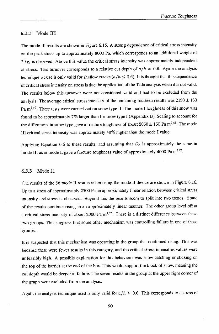
Fracture Toughness
6.3.2 Mode 1111
The mode Ill results are shown in Figure 6.15. A strong dependence of critical stress intensity
on the peak stress up to approximately 8000 Pa, which corresponds to an additional weight of
7 kg, is observed. Above this value the critical stress intensity was approximately independent
of stress. This turnover corresponds to a relative cut depth of a/h 0.6. Again the analysis
technique we use is only valid for shallow cracks (a/h < 0.6). It is thought that this dependence
of critical stress intensity on stress is due the application of the Tada analysis when it is not valid.
The results below this turnover were not considered valid and had to be excluded from the
analysis. The average critical stress intensity of the remaining fourteen results was 2190 ± 160
Pa m 112 . These tests were carried out on snow type II. The mode I toughness of this snow was
found to be approximately 7% larger than for snow type I (Appendix B). Scaling to account for
the differences in snow type gave a fracture toughness of about 2050 ± 150 Pa m 112 . The mode
III critical stress intensity was approximately 40% higher than the mode I value.
Applying Equation 6.6 to these results, and assuming that D0 is approximately the same in
mode III as in mode I, gave a fracture toughness value of approximately 4000 Pa m 112 .
6.3.3 Mode H
The results of the 86 mode II results taken using the mode II device are shown in Figure 6.16.
Up to a stress of approximately 2500 Pa an approximately linear relation between critical stress
intensity and stress is observed. Beyond this the results seem to split into two trends. Some
of the results continue rising in an approximately linear manner. The other group level off at
a critical stress intensity of about 2000 Pa m 112 . There is a distinct difference between these
two groups. This suggests that some other mechanism was controlling failure in one of these
groups.
It is suspected that this mechanism was operating in the group that continued rising. This was
because there were fewer results in this category, and the critical stress intensities values were
unfeasibly high. A possible explanation for this behaviour was snow catching or sticking on
the top of the barrier at the end of the box. This would support the block of snow, meaning the
cut depth would be deeper at failure. The seven results in the group at the upper right corner of
the graph were excluded from the analysis.
Again the analysis technique used is only valid for a/h < 0.6. This corresponds to a stress of
KE

Fracture Toughness
6O00 E Ca Q- 5000
0
0 o
4000 0 U
CO
0
3000 DODD
.2000 DRp 00 0 0
El 0
1000 U)
o 0 I I I •
0 1000 2000 3000 4000 5000 0 Stress (Pa)
Figure 6.16: The 86 mode II results measured using the mode Ii device. The 7 very large results and those with a relative cut depth of less that 0.6 (which corresponds to a stress
of between 2000 Pa and 3000 Pa) were discounted from this analysis.
2000-3000 Pa. Below this a linear relation between stress and critical stress intensity is seen. It
is felt that this relationship is due to Tada relationship being applied when it is not valid. Above
this point, the Tada relation is valid, the results become approximately independent of moment.
Averaging the remaining 14 results gave a critical stress intensity of KJJQ = 2070 ± 300 Pa
m'2 . In mode I snow type V which was used used for these tests was 1.12 times stronger than
snow type I. Scaling the results to snow type I gave K11 = 1840 ± 280 Pa m 112 . This is about
25% larger than the mode I results.
The mode II results were then repeated using the Mode III device. The 33 results of this
experiment are shown in Figure 6.17. For higher stresses the results may stabilise but the
scatter is too large to say for sure. The relative cut depth a/h = 0.6 occurs around a stress of
7000 Pa. Averaging the 14 results with a suitably shallow cut depth gave KJIQ = 2650 ± 460Pa
m 112 , which is about 30 percent larger than the other set of mode II results.
We assume that D0 0.33 m is valid for mode II failure. This gave an approximate fracture
toughness value of 3500 Pa m 112 for the first set of mode II results, and 4600 Pa m' 2 from the
second set. The reason for these trends in the results, and whether they were due to experimental
or analytical techniques is unknown.
91

_ 4000 E CO a-
0 3000
0 0
2000 (I)
Cn 1000 U) a) U)
CO 0
0 2000 4000 6000 8000 10000 12000 14000
Stress (Pa)
Fracture Toughness
Figure 6.17: The 33 mode II stress intensity measurements taken using the mode III device.
6,4 ILiyeirs
6.4.1 Microilayerirtig
The mountain snowpack is a highly stratified material [1]. Even what would be described
as homogeneous snow, is found to consist of many subtly different layers. They are termed
as mircolayers. These are formed by changing weather conditions (temperature, snow fall
intensity, wind and turbulence) during a snowfall event. The experiments discussed so far have
been carried out on what would be described as homogeneous snow, with the cutting carried
out perpendicular to this fine layering. To investigate the influence of this microlayering in so
called homogeneous snow, the mode II and III experiments were repeated but cutting parallel
to the layering.
Mode H measurements, taken with the mode III device, cutting parallel to the layering were
preformed. Tests were performed up to a peak stress of 7200 Pa, which corresponds to an
external weight of 6 kg. This is significantly less than the maximum weight used in the other
mode II experiments. It was found that heavier weights could cause deformation of the snow
sample within the test device. Large deformation meant that the fracture would not run parallel
to the layering. These tests were carried out on snow type V. In mode I this proved to be a
factor of 1.03 tougher than the snow type that the corresponding mode II layer perpendicular
experiments were performed on (snow type IV). Therefore the results were divided by 1.03 to
ON

Fracture Toughness
. 2500
as
CO
E: 0
>
.--6-111 .. ........... 0
Perpendicular to Layers Fit to Perpendicular
CO 500 o Parallel to Layers .Fit to Parallel
CO n. C.)
0 1000 2000 3000 4000 5000 6000
Stress (Pa)
Figure 6.18: Layers have an influence on the Mode ii stress intensity. By fitting linear relations to the data the toughness parallel to the layering is found to be approximately
85% of that perpendicular to the layering.
make them directly comparable to the other mode II results. As the stresses used are quite small
an approximate linear relation between critical stress intensity and stress is seen (Figure 6.18).
This is probably due to the cut depths being deep, and so the analysis technique we use not
being valid in these circumstances. However an analysis technique valid in mode III for deep
cuts could not be found. This means an absolute value of critical stress intensity could not be
found, rather the relation between these two sets of results was found. Fitting linear relations
to both sets of data it was found that they have approximately the same intercept. The gradient
of the fit to the results taken parallel to the layering was 80% of the value perpendicular to the
layering.
This experiment was repeated in mode III using snow type V. The original mode III experiments
were carried out on snow type II. There was a difference of 1.04 in the strengths of these snows.
The results (scaled to account for the difference in snow types) are shown in Figure 6.19. By
fitting polynomials to the data, the critical stress intensity factor parallel to the layering was
found to be 75% of the value perpendicular to the layering.
93

Fracture Toughness
2000
1500- 0
1000-
Perpendicular to Layers C Fit to Perpendicular in 0 o Parallel to Layers
Fit to Parallel .
- 0 I I
: 0 2000 4000 6000 8000 o Stress (Pa)
Figure 6.19: Layers also have an influence on the Mode III stress intensity of snow. By fitting curves to the data the mode 111 stress intensity parallel to the layers is found to be 75 % of that perpendicular to the layers.
6.42 Weak layer
It was shown previously that apparently homogeneous snow fails more easily parallel to the
layering. However most avalanches release via the failure of some form of weak layer or
interface within the snowpack. It is the fracture toughness of this weak layer/interface that is
likely to be the controlling parameter for slope stability. To investigate this a weak layer was
tested in mode III. This layer had been responsible for a number of avalanches on all aspects
in the Davos region around the time the samples were taken. On closer inspection it was found
that there were two distinct weak layers. Both were layers of faceted crystals located above
and below a thin icy crust. Since avalanches ran on both these layers they were both tested.
The results showed the same overall shape as the other mode III results (see Figure 6.20).
The two layers gave similar results, with the critical stress intensity leveling off above a stress
of about 3500 Pa. Again this turnover corresponds to a relative cut depth of approximately
0.6. Considering the 13 results above this turnover gave an average critical stress intensity
Of KJIJQ = 1000 ± 110 Pa m 112 . This is just less than half of the value recorded cutting
perpendicular to the layering in more homogeneous snow, but is approximately double the
value Sigrist measured for the same weak layer [44].
In this case D0 is unlikely to be the same as for homogeneous snow. Therefore we cannot

Fracture Toughness
E 1200 Co IL
1000
800
600-
Co
I:::
• 200
(0 0 E 0
0
0
0 0 0
0 o
0
Cut made above Crust o Cut made below Crust
I I I
2000 4000 6000 8000
Stress (Pa)
Figure 6.20: The stress intensity of the two weak layers was very similar The values level off
above a stress of approximately 3500 Pa. This corresponds to a relative cut depth
of around 0.6. The mean value of the 13 results with a relative cut depth of less
than 0.6 was 1000 Pa m112 .
extrapolate these results to the fracture toughness of the weak layer. It is unclear whether
this difference would be larger or smaller than the factor of 1.8 which was applicable to more
homogeneous snow. In the next chapter, as a first approximation, we assume a weak layer
fracture toughness of 1000 Pa m 112 .
65 Frictfi©n
The fracture toughness experiments described previously have attempted to minimise the influ-
ence of friction. This has involved cutting the snow with string so that the crack faces are not in
contact, keeping any moving parts well oiled, and in the case of the mode II device (where the
snow slid within the metal box) covering the inside of the box with ski wax. However during
the initial basal shear failure stage of avalanche release, the crack faces are pressed together
by the slope normal component of the weight of the snow. This will produce frictional forces
which are expected to increase slab stability.
The influence of friction was investigated by measuring the mode III critical stress intensity
factor under different normal stresses. To do this the mode Ill device was attached on its side

Fracture Toughness
End View Side View
Normal weight
Wire cuts ;rlO I through
snow block
5kg
1 a
weight
Figure 6.21: The friction device; The mode III device was attached on its side to the table. A shear stress of 2500 Pa m112 was produced with a pulley and a 5kg weight. Normal stresses were produced by placing weights on top of the device.
to the table (see Figure 6.21). Shear stress was produced by attaching a piece of string, which
ran over a pulley to a suspended 5 kg weight, to the top section of the box. Different normal
stresses were produced by placing weights on top of the device.
The 5 kg weight produced a shear stress of 2500 Pa. This was kept constant for all the measure-
ments. There was an intrinsic normal stress of about 350 Pa due to weight of the snow and the
box. Additional normal stresses up to 4500 Pa were produced by the addition of weights up to
9 kg. In a field situation it would require a snow depth of approximately 2.5 metres to produce
this amount of pressure on a weak layer. Tests were carried out with larger normal stresses,
but in these cases failure did not occur. The snow was cut through using a thin piece of wire
(diameter < 1 mm) until failure occurred. Thin wire was used so that the crack faces stayed in
contact. The experiment was repeated with no additional weights, and cutting the snow block
with string. This prevented the crack faces from touching. In this case the small normal force
that did exist could not be transmitted through the crack faces as they were not touching. There-
fore the effective normal force was 0 N. The three tests carried out gave a mean critical stress
intensity of Kj1j = 1500 Pa m 112 . Assuming D0 0.33 m, this gave a fracture toughness
of Kjjj = 2700 Pa rn 1 ' 2 . This result is low compared with the other mode III results. It is
suspected that again this is due to the relative cut depth being deeper than 0.6, and so the Tada
analysis not being totally valid. This is an issue for all the data points in this section. However
in mode III this relation is all that is available for calculating fracture toughness. It is expected

Fracture Toughness
that the results can still be used to estimate the coefficient of friction. The results are plotted in
Figure 6.22. At low normal stresses the results are quite consistent while at higher values the
scatter is much larger.
The influence of friction is well illustrated by defining an effective fracture toughness Kapp .
The standard mode III fracture toughness formula is K1ii = where T is the shear
stress acting on the weak layer. When a crack forms, in the presence of friction, the driving
force will be T = (r - Tf) where -rw is the shear stress due to the slope parallel component of
the snows weight, and -rf the opposing stress due to friction. In general the frictional stress Tf is
proportional to the normal stress UN, with the constant of proportionality being the coefficient
of friction i. This leads to
K1jj = (rw - (6.15)
The effective fracture toughness, which neglects frictional stresses in the analysis, and only
accounts for the shear force is then defined as,
Kapp = (6.16)
With increasing normal stress the actual shear stress reduces due to frictional effects, while T w
stays constant. So with higher normal stresses Equation 6.16 will progressively over estimate
the shear stress, which will in turn over estimate the fracture toughness value. On an avalanche
slope, the relative importance of the term [LaN, and hence the amount that Equation 6.16 will
over estimate the fracture toughness, will increase with decreasing slope angle.
The relationship between these two forms of stress intensity is
Kapp = -1-w - PUN
(6.17)
Kjll c is the fracture toughness measured when the crack faces were not touching. This is
assumed to be the value measured when no normal force are acting (2700 Pa rn 1 !2 ). The shear
stress was 2500 Pa. Substituting in these values and fitting Equation 6. l7to the data gave a
coefficient of friction of 0.4. Kapp with ft = 0.3, 0.4 and 0.5 are plotted in Figure 6.22.
The highest normal stress that produced a shear with a measurable ligament size (value of bin
Figure 6.21) was 4350 Pa. This which corresponded to 8 kg of additional weight. Three tests
were carried out with a normal stress of 4850 Pa (9 kg of additional weight). In two of these
97

Fracture Toughness
...... g--0.3
Y.13
6000- i
0 13
co 2000
C ci
0 0 1000 2000 3000 4000 5000
CZ CL CL
Normal stress (Pa)
Figure 6.22: Results offriction experiment. The normal stress varied between 0 Pa and 4350 Pa. Shown are results of Equation 6.17 with three different values of ji. These are 0.3 (dashed line), 0.4 (solid line) and 0.5 (dotted line).
tests shear failure did occur, but only after the block had been cut all the way through (there
was no measurable ligament). In the other case, and in the case of a normal force of 5350 Pa
(10 kg of additional weight), no motion was observed even when the block was cut all the way
through. No motion is expected to be observed when the denominator in Equation 6.17 is less
or equal to zero. This suggests 0.5. It is felt this value of t is the more reliable, as it does
not rely on the Tada analysis, which is not really valid for the range of cut depths observed here.
These values of static friction are likely to have a significant effect on snow slope stability. This
is investigated further in the next chapter.
66 Ctrnch1slirnis
Slab avalanche release is a brittle process. The controlling material property for brittle failure
is fracture toughness. There are three different modes of fracture toughness, all of which are of
relevance to slab avalanche release. Although the fracture toughnesses of other materials have
been well documented, the measurements for snow are quite limited and until recently have
focused on mode I failure.
We report on an experimental program which aimed at measuring all three modes of the fracture

Fracture Toughness
toughness of snow using specially designed boxes. Homogeneous snow consisting of small
rounded particles (size 0.5 mm), hardness one finger to pencil, and a density of between about
250 kgm 3 and 350 kgm 3 was tested. The results were analysed using formula suggested by
Tada et al. as these attempt to account for the specific geometry we use.
Using these relations the critical stress intensity factor were calculated. This was different to
the actual fracture toughness as the samples were not big enough to obey linear elastic fracture
mechanics. However the results could be converted to fracture toughness values by a method
suggested by Sigrist et al. How applicable this method is to our mode II and III experiments is
questionable, but acceptable as a first approximation
Snow was found to be least tough in mode I. The critical stress intensity factor of the snow
used for this test (snow type I) was approximately 1500 Pa m 112 . This corresponds to a frac-
ture toughness of about 2700 Pa m 112 . This is about 30% less than the values measured by
Sigrist[44] on similar snow but using a different technique.
The results of the mode II experiments showed a larger scatter than in mode I. Two different
experimental techniques were used. These two techniques gave critical stress intensity values
of 2000 Pa m 112 and 2600 Pa m112 respectively. These values were 30 and 70% larger than
in mode I. The mode II experiments were repeated cutting parallel to the microlayering that
is found in apperently homogenous snow. It was found that the critical stress intensity was
approximately 20% less when cutting parrallel to the micro layering.
The mode III results were found to be similar to the mode II values. Perpendicular to the micro
layering a critical stress intensity of 2200 Pa m 112 was found. This was approximately 40%
larger than the mode I value. The critical stress intensity parallel to the layering was 75% of
the value perpendicular to the layering. A weak layer which caused numerous avalanches was
tested. This gave a critical stress intensity factor of approximately 1000 Pa m 112 .
In the experiments discussed above we attempted to minimise friction. However friction is of
relevance to real avalanches. To investigate the influence of friction, the critical stress intensity
in mode III under different normal stresses was investigated. Analysing these results gave a
coefficient of friction, (ji) of approximately 0.4 or 0.5. The issue of friction is discussed in
more detail in the next chapter.
all

In this section we critically discuss possible mechanisms of skier triggered slab avalanche re-
lease. In this discussion we quote results of both our computer modelling (Chapter 5), our
fracture toughness experiments (Chapter 6) and from other people's work. Basal shear friction
is investigated in Section 7. 1, and in common with other snow properties, is found to be highly
variable. A coefficient of friction (pt) for dry snow of about 0.7 seems to be a typical value. The
size of the critical shear band is considered in the following Section (7.2). Estimates of this
value in the literature vary over about two orders of magnitude, from a few tens of centimetres
to a few tens of metres. We estimate the critical shear band radius to be of the order of ten
metres. Although it is conceivable that this could be produced by an explosive charge, it is
difficult to see how a single skier could produce a shear band of this size. However as skiers do
trigger slab avalanches, a triggering mechanism must exist.
We discuss two alternative triggering fnechanisms. The first mechanism, which is considered
in Section 7.3, is that localised damage caused by the skier can interact with the natural pre-
existing distribution of shear cracks. In some areas this can have a strong knock down effect
on stability. The other triggering mechanism, discussed in Section 7.4, is the solitary wave.
This is caused by the compressive failure of the weak layer. These are easy to initiate and is a
commonly observed in flat terrain.
71 Fii1ci©ini
Initially the magnitude of basal friction is investigated. The frictional resistance acting on an
avalanche can be expressed as a power series of velocity [48].
Fr A r +BrV+CrV2 (7.1)
where v is the velocity, Ar is the dry frictional force, Br is the viscous friction coefficient and
Cr is the turbulent friction coefficient. During avalanche release the velocities are low (v 0),
100

Slab Avalanche Release Mechanisms
so the frictional forces are mainly due to dry friction, Fr A r. Dry friction consists of two
terms: Coulomb friction (which is proportional to the normal force) and adhesion (which is
proportional to the contact area) [48].
A r = pN + egsA (7.2)
where i is the coefficient of Coulomb friction, N is the normal force, e is the adhesion co-
efficient, g is gravity and SA is the surface area. The adhesion term is due to the growth of
bonds. In the following we consider the most unstable situation, that is before any bond growth
has occured. Therefore the adhesion term is ignored and the frictional force assumed to be
proportional to the normal force
Fr [LN. (7.3)
We estimate i for dry slab from various sources.
Initially an experiment carried out by Alex van Herwijnen is considered. This is labelled as
test CTC and described on page 207-211 of his PhD thesis[ 49]. He records the motion of a
section of slab during a compression test on a thirty degree slope. This motion is caused by
the sudden collapse of a layer of faceted crystals. Since the motion is due to a collapse there is
both a slope perpendicular and slope parallel components of the motion. By carefully analysing
the motion, the displacement, velocity and acceleration profiles of the slab were determined.
Although the experiment was designed to investigate fracture propagation, enough information
is presented to estimate the coefficient of friction. The maximum slope parallel velocity was
0.38 ms -1 . One tenth of a second later this had dropped in an approximately linear manner
to 0.16 ms'. This corresponds to an average deceleration of 2.2 ms -2 . This experiment was
carried out on a slope of 0 = 300. The force per unit mass acting on the slab in a slope
parallel direction was g sin 0. However slope perpendicular motion due to the collapse of the
weak layer needs to be considered. During the period being considered, there was also a slope
perpendicular deceleration of 1.6 ms— 2 . This means that the normal force per unit mass was
1.6 + g cos 0. Therefore a frictional force per unit mass of (1.6 + g cos 0) resisted this motion,
while a force per unit mass of g sin 0 would encourage the motion. These forces sum to produce
a slope parallel deceleration of 2.2 ms— 2. Solving this corresponds to a coefficient of friction
of /2 0.7.
Friction can also be estimated from the minimum slope angle on which avalanches occur. Gen-
101

isms
4sZ 21 Slab
I -. - Weak Layer X x=0
Ground
End;
IT ext
Region
Figure 7.1: A shear band is an extended length or area of half lengthlradius 1, where the shear
strength of the weak layer has dropped of to its residual frictional value T,
erally dry snow slab avalanches do not release on slopes less than about 30 degrees. This
implies that generally tt > 0.5. Occasionally however they do occur. In a study of avalanches
in the European Alps from the notorious winter of 1999, it was found that 4 out of approxi-
mately 800 avalanches released on slopes with a maximum inclination of less than 30 degrees
(two of these occurred at 26 degrees, one at 27 degrees and one at 29 degrees). This indicates
that u can sometimes take values below 0.5.
We see from the discussion above that like other snow properties, coefficient of friction () of
dry slab can take a wide range of values. This agrees with the work of Casassa et al. who found
coefficients of friction of between 0.58 and 0.84 [48]. A typical coefficient of friction could be
taken as p = 0.7. The coefficient of friction reported in the previous chapter is smaller than
the majority of the values mentioned here. It is suspected this is mainly because the process of
cutting with a wire is likely to produce smoother (lower t) crack faces than would be produced
naturally. Also as the normal stresses were very high, the relative contribution of any adhesion
term (which may be present in the other results) will be negligible.
72 Shear Bands
In this section we investigate the critical size of a shear band in different scenarios. We define
a shear band as a region over which the shear strength of the weak layer has dropped of to it's
residual frictional value Tr (see Figure 7.1). For simplicity we assume a single shear band in an
102

Slab Avalanche Release Mechanisms
otherwise homogeneous weak layer. A slab depth of 0.5 metres, a slab density of 200 kg m 3
and a weak layer fracture toughness of 1000 Pa m 112 are assumed.
7.2.1 Simple Shear Band
The simplest calculation of critical shear band size is via the direct application of the Griffith
relation. This is
Kc = . (7.4)
where r = pg(d - d') sin (slope parallel shear stress) and Kc is the weak layer fracture
toughness in shear. This relation is derived in one dimension, so a corresponds to the critical
crack half length, and it assumes that there is no residual frictional force. For a slope of 38
degrees this gives a critical size half length of approximately 0.9 metres.
However the results change significantly if basal friction is incorporated. In this case the effec-
tive shear stress will be r = pg(d - d) (sin 0 - cos 0). We assume a characteristic value of
basal friction of u = 0.5. This is at the low end of the distribution of i. However this shows
that even assuming the minimum likely value of u, friction is still highly significant. The vari-
ation in critical half length with slope angle is shown in Figure 7.2. However this assumes that
the Griffith relation (Equation 7.4) is valid, we later show this is unlikely for such a large shear
band. For a slope angle of 38 degrees, the critical half length is about 7 metres. This is almost
an order of magnitude larger than the result without friction. Taking a value of friction from the
high end of the distribution has an even more profound effect. If p = 0.8 then avalanches are
not possible on slope angles less than about 39 degrees. We see that neglecting friction in the
calculation of critical shear band size is likely to seriously underestimate the true value.
7.2.2 Deviations from Griffith's Criterion for Large Shear Bands
There are two problems with the above method of calculating critical shear band size. Firstly we
use the Griffith relation which is only valid in one dimension. Real shear bands are essentially
two dimensional objects. A second dimension is likely to increase critical shear band length by
a numerical factor of about two, depending on the shape of the shear band. More importantly the
derivation (outlined in Section 6.1) of the Griffith relation assumes that the material dimensions
are significantly larger than the crack size. However, when friction is incorporated, the critical
shear band size is likely to be larger than the slab depth (a > d - d'). Under these conditions
103

Slab Avalanche Release Mechanisms
Critical shear band sizes
No friction
Friction l.L=0.5
cu 6 CD -c
C., 2
00 30 40 50 60
Slope Angle (degrees)
Figure 7.2: The variation in critical flaw size with slope angle should friction be ignored and ft = 0.5, as predicted by the Griffith relation. If i = 0.5 then critical shear band size diverged for a slope angle of 27 degrees.
the relation between fracture toughness and critical shear band size changes.
Here we derive an two-dimensional expression for the critical shear band size, assuming it to
be significantly larger than the slab thickness. We call this the thin slab approximation. Our
derivation is similar to that given in Section 4.4, but is slightly more complicated because we
use dimensional variables.
The surface energy associated with a circular shear band of radius a will be
E = 'ylra2
(7.5)
where 'y is the surface energy per unit area of the material. The change in potential energy due
to the formation of the shear band is the displacement times the stress, integrated over the area
of the shear band. As the situation has circular symmetry a polar coordinate system can be used
for this step is
jo Jo
a p2ir = —r I ru(r)dçbdr (7.6)
Assuming no 4 dependence then Equation 4.33 becomes equivalent to
Iiii+ Iii 7 ô2 n
2 (.(9x2Dy2) (TextToo). (7.7)
20
18
16
14
- 12 CZ
D 10 CU
104
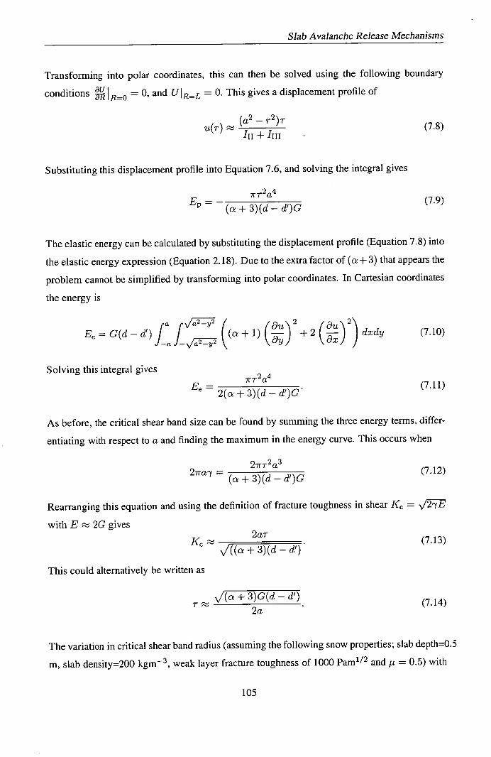
Slab Avalanche Release Mechanisms
Transforming into polar coordinates, this can then be solved using the following boundary
conditions = 0, and UIRL = 0. This gives a displacement profile of
(a2 - r2)r (7.8)
u(r) hi + Iiii
Substituting this displacement profile into Equation 7.6, and solving the integral gives
irr 2 a 4 E = - (7.9)
(a+3)(d—d')G
The elastic energy can be calculated by substituting the displacement profile (Equation 7.8) into
the elastic energy expression (Equation 2.18). Due to the extra factor of (a + 3) that appears the
problem cannot be simplified by transforming into polar coordinates. In Cartesian coordinates
the energy is
a ./a2—y2 (a+i)(—) +2(
,,U)
— jdxdy Ee = G(d - d') f_a f (
2 2\
\8:J/ OX J
Solving this integral gives irr2 a4
Ee = 2(a + 3)(d - d')G
(7.10)
(7.11)
As before, the critical shear band size can be found by summing the three energy terms, differ-
entiating with respect to a and finding the maximum in the energy curve. This occurs when
2ir'r2 a3 2ira'y =
(a + 3)(d - d')G (7.12)
Rearranging this equation and using the definition of fracture toughness in shear K =
with E 2G gives 2ar
K ______________ . (7.13) \/((a + 3)(d - d')
This could alternatively be written as
/(a + 3)G(d - d') (7.14)
2a
The variation in critical shear band radius (assuming the following snow properties; slab depth=0.5
m, slab density=200 kgm 3 , weak layer fracture toughness of 1000 Pam 1/2 and IL = 0.5) with
105

Slab Avalanche Release Mechanisms
slope angle is shown in Figure 7.3. Also shown is the critical half length predicted (in one
dimension) by relation 7.4. It should be noted that all these critical shear band calculations
assume linear elastic fracture mechanics, and do not consider energy dissipated because of ma-
terial plasticity. Therefore all sizes quoted should be considered lower limits for the critical
shear band size.
Bazant et al.[50] and Louchet et al. [51] also consider deviations from the Griffith relation
due to the slab being thin relative to likely critical shear band size. Bazant et al. obtain the
expression __________
- d') ./2E(d T . (7.15)
a
As a typical value of c is 0.3, this is expression is very similar to Equation 7.14. However the
relation that Louchet et al. derive is different. One cause of this difference is that they consider
the elastic energy stored in the substrate. We do not consider this because, as shown in Section
2.2, for a thin slab the properties of the substrate are not relevant. This implies that no energy
is stored there. Another cause is the displacement profile used. Louchet et al. assume the shear
band displacement profile to be the same as that found around a crack in an infinite medium. In
the above calculation, the displacement profile measured by McClung [52], and also predicted
numerically with our computer model, is assumed.
7.2.3 Field Evidence
There is field evidence which indicates that friction needs to be considered when calculating
critical shear band size. When carrying out fracture experiments for his PhD thesis [49], Alec
van Herwijnen observed that a skier produced a shear fracture with a size of 3.0 ± 0.2m. We
assume that the shear band is approximately circular and has a radius of 1.5.0 ± 0.1m. This did
not propagate further, indicating it was less than the critical size. The snow properties at this
location were well recorded, allowing a good estimate of critical shear band size to be made.
The slope angle was 41 degrees, the slab depth was 39 cm and the slab density 118 kgm 3 .
By assuming that for brittle failure stress is proportional to strain, that the strain at failure is
relatively constant, and by estimating shear strength of the weak layer the fracture energy could
be estimated. In this case this was estimated to be 0.17 J m 2 . The Young's modulus (E) for
this density of snow is about 500 kPa [5]. Using the relationship between the Young's and shear
modulus (E = 2C(1 + ii)), implies a shear modulus of about 200 kPa. This gives a fracture
toughness of 260 Pa m 112 . To see if this is a reasonable value, we extrapolate our fracture
106

Slab Avalanche Release Mechanisms
30
Critical shear band sizes CD
24 Griffith
E 22 \ Thin Slab, 2D 20
.18 U)
16- C - -° 12-
10- .c 8- U)
0 co 4-
...
or'
28 30 32 34 36 38 40 42 44 46 48 50
Slope Angle (degrees)
Figure 7.3: The variation of critical flaw size with slope angle. The dotted line shows the one dimensional critical half length as predicted by the Griffith relation (Equation 7.4. The solid line is critical shear band radius of the thin slab approximation (Equation 7.13).
toughness results to this density of snow. We assume the results of Sigrist [5], that fracture
toughness is proportional to density to the power of 2.4, is valid in shear as well. Using this we
scale our results (Kjj 3400 Pa m 112 parallel to the layering for a density of 300 kgm 3 ) to
a density of 118 kgm 3 . This gives a fracture toughness of about 360 Pa m 112 . However this
estimate is for homogeneous snow, and so it is not surprising that it is larger than the fracture
toughness of a weak layer.
Using the Griffith relation and neglecting friction, a critical shear band size of approximately 40
cm is found. If a coefficient of friction of 0.5 is assumed then the critical shear band size is likely
to be significantly larger than the slab depth. This means that the thin slab relation (Equation
7.13) will be applicable. This gives a critical flaw radius of approximately 1.2 metres. The
situation is complicated as additional shear forces, produced by the skier, are not accounted
for, and a large hole had been dug at one side of the region. These facts are likely to reduce
the critical size. On the other hand we assume a low coefficient of friction. Choosing a larger
coefficient of friction is likely to increase critical shear band size. This emphasises in a practical
way that friction, and critical flaw size quite easily being larger than the slab depth should to be
107

Slab Avalanche Release Mechanisms
considered when calculating critical shear band size.
73 I[teradirniis of Skfler Damage with Txisthiig IFilaws
When friction is incorporated into shear band models, the critical radius is found to be of the
order of 5 metres. Although it seems feasible that an explosion could produce a shear band of
this size, it is harder to see how a single skier could do this. Here we discuss two alternative
ways that a single skier could feasibly trigger a slab avalanche.
Firstly we propose that skier triggering may result from the interaction of localised damage
caused by the skier, with the complex distribution of elastically coupled cracks which is as-
sumed to lead to natural failure. A skier is likely to cause localised damage to the weak layer.
The scale of this damage is small compared to the critical flaw size and, in general, this local
damage will have little effect on slope stability. However in some locations, local damage has a
very strong knock down effect on slope stability. If supporting regions at the edge, or between,
existing shear bands are destroyed, it is possible that the shear bands will reach the critical size,
leading to avalanche release. This distribution and influence of these "hotspots" was explored
in some detail with our numerical model in Section 5.6.
However such "hotspots" are not just a theoretical concept, their existence has been known
among avalanche practitioners for a long time. The principle is observed in the field when a
number of skiers safely descend a slope, then an unfortunate skier hits a hotspot, and the entire
slope releases. In reality the phenomenon of hotspots tends to occur a few days after heavy
snow fall events. This time period may allow significant healing and creep to occur within
the weak layer. However non-uniform internal stresses are likely to remain, and as our model
shows, it is these that are likley to produce some areas which are more likely to release than
others.
74 Solltary Waves
The other mechanism which can be responsible for avalanche release is the solitary collapse
wave. These are also known as whumpfs, especially by practitioners. A solitary wave occurs
when a weak layer collapses under the weight of the overlaying snowpack, and the snowpack
settles vertically downwards (Figure 7.4). This often produces a characteristic "whumpf' noise.
108

Wave Propagation
Compression Slab
Untractured weak layer
Weak layer is crushed
Figure 7.4: A schematic of a solitary wave. Compressive failure of the weak layer creates a solitary wave which propagates along the slab/weak layer
In some cases vertical settling of the snowpack can be directly observed. The process propa-
gates because the overlaying slab at the edge of the collapsed region is bent, stressing and
causing further collapse of the weak layer. This bend, or solitary wave propagates outwards.
Following the work of Johnson et al.[53], Johnson et al.[54] and Lakinger[37], Heierli[55] and
Heierli and Zaiser [56] developed a theory to describe this process.
Whumpfs are a common phenomenon in flat terrain. Using geophones buried in the snow,
Johnston et al. measured the fracture speed of a whumpf in Bow Summit [54]. The weak layer
was a layer of buried surface hoar under 39 cm of slab with a density of 189 kgm 3 . The weak
layer collapsed, leading to the vertical settling of the slab by approximately 1 mm. The collapse
was initiated by a person walking on the snow. The solitary wave traveled past the geophones
at a constant speed of 20 ± 2 ms -1 . Given these snow properties, Heierli's theory predicts a
velocity of 22 ms -1 [55], in good agreement with the experimental results. This result supports
but does not prove Heierli's theory.
There is an increasing amount of evidence to suggest there is often a compressive compo-
nent to weak layer failure. For his thesis [49] Alex van Herwijnen recorded shear fracture in
rutschblocks (where a rutschblock is an isolated column of snow approximately one metre by
two metres and with a variable height depending on the depth of the weak layer which are
traditionally used to evaluate slope stability) and on skier tested slopes. In fourteen out of fif -
teen shear fractures there was a small slope perpendicular collapse which either preceded or
occurred at the same time as larger slope parallel sliding. In general the slope perpendicular
collapse was of the order of 0.5cm.
109

Slab Avalanche Release Mechanisms
van Herwijnen also studied video recordings of externally triggered slab avalanche release. By
measuring the time between the trigger (usually an explosive charge) and slab rupture, and
estimating the dimensions of the release zone, the fracture propagation speed through the weak
layer could be calculated. The rate of expansion of an unstable shear band is likely to be half
the velocity of a shear wave [17]. van Herwijnen [49] finds that the speed of the fracture better
matches the speed of a solitary wave than predicted expansion of an unstable shear band.
Solitary waves can also explain the phenomenon of remotely triggered avalanches. A remotely
triggered avalanche occurs when a trigger releases a slab, but is not within the area that initially
fails. They could be caused by a solitary collapse wave propagating into an area which is more
suitable (e.g. due to a larger slope angle) for avalanche release. The weak layers associated
with remotely triggered avalanches tend to contain large crystals. This is exactly the type of
weak layer that would be suitable for vertical collapse and solitary wave propagation. In one
study of avalanche type and associated weak layer properties, for 96% of solitary waves and
remotely triggered avalanches either depth hoar, buried surface hoar, or facets were visible at
the weak layer [53]. For non remotely triggered avalanches, these crystals types were visible in
only 49% of cases.
Whumpfs are not just local phenomena. Once initiated they are able to travel large distances,
sometimes into areas more suitable for avalanche release. Den Hartog quotes an example in
Antarctica where a whumpf (referred to as a firn quake in this case) was recorded to travel
for over five miles [57]. In their measurements from Bow Summit, Johnson et al. report that
the solitary wave they produced continued until an abrupt change, in slope angle or to where
vegetation protruded through the snowpack [54].
7.4.1 Energy Considerations
To investigate the possible involvement of solitary waves in skier triggered avalanches, the
energies associated with a solitary wave and a shear band are considered. We assume a quasi
one dimensional situation. This is the slope is totally homogeneous in the y direction, and
a shear band/solitary wave expanding in the x (across slope) direction. We use dimensional
variables. All energies are quoted per unit length in the y direction. We assume both phenomena
are centred at x = 0 and have half length 1. The following typical snowparameters are assumed:
slab depth (d—d')=0.5 m, slab density p = 200 kgm 3 , coefficient of friction t=0.5 and a slope
angle 0= 38 degrees. If we assume a typical fracture toughness of 1000 Pam 112 , and a typical
110

2
E
0
> >. (
-2 LU
0 ci:
I Solitary WaJ
Slab Avalanche Release Mechanisms
Young's modulus of 1 MPa, then this implies (via Equation 6.2) a fracture/surface energy y=0.5
Jm 2 . This is significantly larger than the value reported in Section 7.2.3, but acceptably close
given the variability of snow properties.
Firstly we consider the solitary wave. We note this is not a detailed calculation, and various
important approximations are made. However we can justify these approximations by noting
that the results are strongly dependent on the values of some highly variable snow properties
which are assumed. An error of a few tens of percent due to the approximations we make is not
significant compared to the range of results that can be achieved by choosing different snow
parameters. The two main approximations we make are that the solitary wave is quasi one-
dimensional, and that collapse occurs in a slope perpendicular direction. These approximations
are made so that the results of Heierli and Zaiser [56] (who developed a theory for solitary
waves in the flat) can be applied here . Here we use their results, the only difference being that
in our case the gravity acceleration action in the slope perpendicular z direction is assumed to
be g cos 0. A vertical settling height of 1mm as was observed by Johnson et al.[53] at Bow
Summit is assumed. A critical half length of about 0.6 metres is obtained. This corresponds to
an energy barrier of 0.5 Jm 1 (see Figure 7.5).
0 1 2 3 4 5 6 7
Solitary Wave/Shear Band Half Length (m)
Figure 7.5: The energy released by a solitary wave and a shear band assuming various "stan-dard" parameters (see test for details). The solitary wave has a smaller energy barrier, and critical size.
We now calculate the energy associated with the shear band. The thin slab approximation is
used. We use a one dimensional version of the derivation given in Section 7.2.2.
111

Slab Avalanche Release Mechanisms
The surface energy associated with the shear band is
E = 21'y (7.16)
where 1 is the half length of the shear band.
In dimensional coordinates the displacement profile of a one dimensional shear band is given
by (1 2 _x2 )pg(sin0 - COS 0)
u(x)= 4G
(7.17)
Multiplying this by the shear force, and integrating over the length of the shear band gives the
energy released by the shear band
E = _ p2 g2 1 3 (d_ d') (sin O - 0.5 COS O) 2 (7.18)
Substituting the displacement profile into Equation 2.20, the elastic energy associated with the
shear band is found to be
Ee = P29213 (d - d) (sin 0 - 0.5 cos 9) 2 (7.19)
This is half of the potential energy. Therefore the total energy associated with the shear band is
ETotal = 21-,'— 1 2 2 13 g (d—d')(sinO-0.Scos0) 2 (7.20)
Assuming a shear modulus G of 0.5 MPa, gives a critical length of about 3 metres, with an
energy barrier about 1.5 Jm 1 . Both the critical length and energy barrier are about three times
larger than for the solitary wave (Figure 7.5). In this example the coefficient of friction assumed
is a the lower end of the distribution. The collapse height of the solitary wave is assume to be
1 mm found by Johnson et al, rather than the typical value of 5 mm found by van Herwijnen.
It is seen that although the parameters we chose encourage shear band propagation, the solitary
wave is still significantly easier to initiate.
A more detailed theory of coupled compressive and shear failure of a weak layer is presently
being developed by Heierli and Zaiser [58]. Their results reduce to those of McClung [17],
for the limiting case of there being no compressive failure. Their conclusions are also that in
general compressive failure significantly reduces initiation energy/critical size.
112
Slab Avalanche Release Mechanisms
It should be noted that solitary waves require a weak layer which is collapsible. This will not
always be the case. However if the weak layer properties do suit collapse (e.g a layer of large
weak crystals) then a possible scenario for slab avalanche release goes as follows: A solitary
collapse wave is easily initiated by a skier. This solitary wave then starts spreading through the
weak layer. With compressive failure comes the loss of shear strength. After collapse, slope
parallel sliding releases more energy, which further encourages propagation. The collapsed
region soon reaches the critical shear band size. The fracture continues to expand, probably as
a combination of both compressive collapse and brittle shear failure. This continues until the
tension in the slab becomes too large, and tensile rupture then occurs.
705 Condllasoiin
Friction plays an important role in slab avalanche release. The coefficient of friction for dry
slab can be estimated from a number of sources. It is found to be a variable quantity, but value
between 0.5 and 0.8 seem typical. The effect of friction, and the fact that the critical shear
band size is likely to be large relative to the slab depth, need to be considered when calculating
critical shear band size. When these effects are considered, the critical shear band size is of the
order of ten metres. It seems unlikely that a single skier could produce such a large damaged
area. We investigate two alternative triggering mechanisms. The first process is that local
damage caused by a skier interacts with the complex distribution of natural shear cracks. It was
shown using the computer model that local damage at certain locations can have a strong knock
down effect on slope stability. The other triggering mechanism is the solitary collapse wave,
or whumpf. This is due to the compressive failure of the weak layer, which leads to the loss
of shear strength. Solitary waves only need a small amount of energy to initiate and can travel
large distances.
A wide variety of behaviour is associated with slab avalanche release. This variety would be
very difficult to explain if it is assumed that slab avalanche release is due to a single mecha-
nism. However the two processes we discuss here, combined with a highly variable coefficient
of basal friction can explain this variety of behaviour. Examples of the different behaviour
observed are; a skier triggering a well track slope, solitary waves which lead to slope failure,
solitary waves which don't lead to slope failure and remotely triggered avalanches.
113

Chapter :
(
In this thesis we investigated dry snow slab avalanche release using various computational, the-
oretical and experimental techniques. Slab avalanche release is essentially a fracture mechan-
ics problem, meaning that for complex (realistic) situations analytical solutions do not exist
and numerical models have to be used to study the behaviour. In this thesis we report on the
development and results of a cellular-automaton type computational model of slab avalanche
release.
A simple snowpack consisting of three layers; the substrate, a weak layer and the overlaying
slab was modelled. The weak layer was modelled as a displacement-softening interface. Vari-
ability was introduced by discretising space, and assigning to every site a random basal shear
strength. Stress redistribution from weak to strong regions was expressed in terms of the sec-
ond order gradient of the displacement across the weak layer. The model allowed for rupture
of the slab to occur when the stress within the slab, expressed as the first order gradient of
displacement, reached a critical value. Our investigations led to the following conclusions:
o Variability within the weak layer had a strong knock down effect on slope stability. This
knock down effect could be approximated by (S e) 0.28 (Sm) (0/(Sm ) 2 ) 045 .
o The length scale of the variability also had a strong knock down effect on slope stability.
o The critical stress at which slope failure occurs was a random variable with an approx-
imately Gaussian distribution. The width of this distribution increased with decreasing
slope size, while the average critical stress increased. This implies that smaller slopes are
both more stable but less predictable.
o The critical flaw which leads to natural avalanche release was neither an extended shear
band, nor a point like deficit. Instead, damage clusters of widely varying sizes emerged
and the distribution of failed sites had features of a fractal set.
o As the external load increased, global failure was preceded by small precursor events,
which may be detectable by acoustic emissions. These precursor events came in the form
114

Conclusions
of bursts superimposed on a background 'creep' activity. Similar patterns of acoustic
emissions have been recorded for avalanche slopes, although their interpretation is not
conclusive [38], [39].
o Snow is a time dependent material [9] [10], and this was introduced into the model by
allowing damaged regions to regain their initial strength over time. However this was
found to make little difference to the critical stress.
• This implies that internal stresses are crucial for slope stability. During loading of the slab
a pattern of large deficit zones supported by a few key anchoring points develops. These
anchoring points correspond to strong, but at the same time highly stressed, parts of the
weak layer. Slope failure was triggered by the overloading of one of these anchoring
points.
• In our model the slab rupture strength did not influence slope stability, but has a signif-
icant effect on avalanche size. This implies that rupture is a separate process occurring
subsequent to shear failure.
o An unstable slope was likely to naturally develop a complex pattern of shear bands.
Generally, local damage to the weak layer caused by a skier had little effect on slope
stability. However in a few locations this local damage did have a very strong knock
down effect on slope stability. These regions where triggering is highly likely have been
called hotspots.
o Field observations show that slab avalanche sizes are power law distributed [23] [24].
It was shown that this size distribution could result from the power law distribution of
controlling parameters that has been observed in the field [24]. Another possibility is that
this distribution is due to geomorphological statistics. However our model indicates that
it is unlikely to be due to dynamic critical phenomenon.
However, the development of our model relies on some strong approximations. Our analysis of
the stress redistribution factor assumed that the depth of the slab (d - d') is small in comparison
with the correlation length . If this is not the case (which is entirely possible) our model will
over-estimate the impact of the fluctuations. Also our model does not account for the different
failure characteristics that occur at different strain rates (ductile at low strain rates, brittle at
high). However we emphasize that we do not attempt to model all aspects of slab avalanche
release in detail, but more to investigate the main processes. Despite the approximations used
115

Conclusions
it is felt that the model in its present form successfully captures all the main aspects of slab
avalanche release.
Although we believe that the model captures the main aspects of avalanche release there may
be significant differences between our model and reality. This is to some extent due to what we
model; a uniform slope. Local topography and slope scale variations are likely have significant
influences on avalanche release. This can lead to misleading results. For example our model
suggests that slab strength will not effect slope stability when in reality this is not the case. This
may be because on small slopes the strength of the slab is enough to support the entire slope.
Alternatively there may be hidden correlations between parameters we consider independent.
For example a harder slab may imply a stronger weak layer. Therefore the results discussed
above should be treated with care, as they are model outputs, rather than field observations.
The results of an experimental study to determine the fracture toughness of snow were reported.
Specially designed boxes were used for these experiments. Snow typical of that which produces
slab avalanches was used for these experiments. An analysis technique which was specific to
the geometry of the tests was used. The main results of this experimental program were:
Snow was found to be least tough in tension (mode I). The fracture toughness of homo-
geneous snow of a density about 300 kgm 3 was found to be about 2.8 kPa m 112 .
o The fracture toughness for both forms of shear failure (mode II and III) was found to be
of the order of 4 kPa m 112 . This is about 40% larger than the mode I value.
o Even apparently homogeneous snow consists of many subtly different layers. The values
quoted above are for failure occurring perpendicular to this fine layering. In all cases, the
fracture toughness parallel to this layering was about 80% of that perpendicular to the
layering.
o The fracture toughness of a weak layer in shear (mode III) was found to be between about
1 and 2 kPa m 112 . This is of the order of one half of the value for homogeneous snow we
tested.
There was a large amount of scatter in the results. In the end alot of the measurements were not
valid due to our analysis technique only being valid for shallow cracks (a/h > 0.6). Therefore
the values of fracture toughness quoted above should be regarded more as order of magnitude
values rather than absolute values.
116

Conclusions
In the final chapter various mechanisms for skier triggered avalanches are discussed. The coef-
ficient of dry friction p is an important parameter. The value of p can be estimated from various
sources, and is found to be highly variable, but jt=0.7 seems to be a typical value. Incorporating
friction into shear band models gives a critical size of the order of ten meters.
The range of behaviour associated with slab avalanche release suggests that more than one pro-
cess can lead to avalanche release. We discuss two possible mechanisms for skier triggered slab
avalanche release. The first mechanism is that very localised weak layer damage caused by the
skier can interact with the complex pattern of internal stresses. In a few locations this can have
a very strong knock down effect on stability. These areas are called "hotspots". The existence
of hotspots has been known to avalanche practitioners for a long time. This mechanism can
explain why a skier, who is unlucky enough to hit a hotspot, can trigger a slope that numerous
other skiers have safely descended.
The other possible triggering mechanism is the solitary wave, or whumpf. This is caused by
the compressive failure of a weak layer of large crystals such as facets, depth hoar or buried
surface hoar. With compressive failure comes the loss of shear strength. Solitary waves do not
require much energy to be initiated, and can travel large distances. They can travel from their
initiation point onto areas more susceptible to avalanche release, explaining the phenomenon of
remotely triggered avalanches. Also, if the coefficient of friction is high enough, it can explain
why slopes can whumpf and crack, but not release an avalanche.
The processes which lead to slab avalanche release are not well understood. One problem is
that no single one process can explain all the phenomena associated with slab avalanche release.
Investigation of which (if any) mechanism is dominant would involve the detailed study of weak
layer properties and behaviour. This is made difficult by many factors. Avalanches are rare and
non-reproducible events [1]. Access to starting zones at times of low stability (the times of most
interest) is dangerous. The important processes occur in the weak layer, which is usually hidden
by tens (or hundreds) of centimetres of overlaying slab. To make the issue more complex the
processes associated with avalanche release range over about 6 orders of magnitude in scale,
from the damage of individual bonds between snow crystals (scale 0.1 mm) to large scale
avalanche release (scale 100 m). In this thesis we have made qualitative statements about slope
stability, avalanche size distribution, and release mechanisms. However, predicting the time,
location and size of an individual avalanche is still not possible. It appears that developing and
verifying a detailed theory of avalanche release in such a complex material as snow, covering
117

Conclusions
all the processes, from individual bond failure to slope release will remain very challenging [1].
118

IMUIDMI'll ~~E,
91 Tablie 1
Typical physical parameters for the snow on an avalanche prone slope are outlined below.
Parameter Typical value Range Reference
slab depth (d - d') 0.5m 0.3 - im Schweizer 1999 [3]
slab density p 200 kg/rn3 100-300 kg/M3 Schweizer 1999 [3]
shear modulus C 0.5MPa 0.1-5MPa Schweizer 1999 [3]
ratio shear modulus G/ peak strength Tm
100 20-200 Schweizer 1999 [3]
ratio peak strength Tm!
residual strength Tr
1.5 1.25-2 Schweizer 1999 [3]
ratio peak strength standard deviation 0m/
average peak strength (Tm )
1 0.6-2 ______________
Conway and Abrahamson 1988[ 21 ]
correlation length of strength variations
irn 0.2-1.3m Conway and Abrahamson 1988[ 21 ]
displacement to failure v 4mm 1-10mm McClung 1979[ 17 ]
loading time Text/Text iO4 s 10 - 106s
characteristic sintering time t. 10 s 1 - 105s
Table 9.1: Typical values and ranges of the physical parameters entering the model
119

Chapter 10 Snow used
101 Tablle2
Snow Date Form and Hand Density KIQ Tests Performed collected size hardness (kg rn 3 ) (Pa rn 1
!2 ) (number of test carried index out in brackets)
I 10th Jan small rounds 1 Finger! 291 1480+320 Mode I standard (47) Pencil (272-353)
II 24th Jan small rounds 1 Finger! 323 1590±230 Mode ifi standard (56) (0.25-0.5mm) Pencil (299-363)
III 9th Feb faceted crystals Pencil Mode III weak Layer (19) (1mm)
IV 23rd Feb small rounds 1 Finger! 290 1620±240 Mode II using Mode III (0.3-0.6mm) Pencil (254-314) device (33)
Mode II standard (86) V 3rd Mar small rounds 1 Finger 330 1660±150 Mode II parallel
(302-340) to microlayering (18) Mode III parallel
to microlayering (15) VI 14th Mar small rounds Pencil 286 Mode III friction (33)
slight form (255-306) (0.2-0.5mm)
Table lOit: A brief description of the snow used for the fracture toughness experiments. Hard-ness as defined by the hand hardness index. For Density the mean value is given in the first line, and the maximum and minimum values measured for that snow are given in brackets. For mode one critical stress intensity (KJQ) the mean plus and minus one standard deviation is given. In the final column which tests, and how many were carried out is listed.
120
Publications
Articles in International Journals
B. Fyffe, and M. Zaiser, The effects of snow variability on slab avalanche release, Cold Reg.
Sci. Technol., 40 229-242 (2004).
B. Fyffe, M. Zaiser, and E. C. Aifantis, Shear bands and damage clusters in slope failure-A one
dimensional model, J. Mech. Behav. Mater , 15 185-202 (2004).
B. Fyffe, and M. Zaiser, Interplay of basel shear fracture and slab rupture in slab avalanche
release, Accepted for Cold Reg. Sci. Technol. Special edition, (2006).
Papers in Colference Proceedings
M. Zaiser, B. Fyffe, P. Moretti, A. Konstantinidis and E.C. Aifantis, Pinning and propagation
of interface cracks in slope failure: 1D and 2D considerations, In: Modelling of Cohesive-
Frictional Materials, Eds. P.A. Vermeer, W. Ehlers, H.J. Herrmann & E.Ramm, Taylor and
Francis, London 2004, pp. 435-446.
121
References
J. Schweizer, B. Jamieson, and M. Schneebeli, "Snow avalanche formation.," in Review
of Geophysics, vol. 41(4), p. 1016, 2003.
B. Jamieson and C. Johnston, "Snow characteristics associated with avalanche accidents," in Canadian Geotechnical Journal, vol. 29, pp. 862-8667 1992.
J. Schweizer, "Review of dry snow slab avalanche release.," in Cold Regions Science and Technology, vol. 30(1-3), pp. 43-57, 1999.
B. Jamieson, "Fracture propagation and resistance in weak snowpack layers," in Avalanche News, vol. 61, pp. 36-43, 2003.
C. Sigrist, J. Schweizer, H. Schindler, and J. Dual, "On size and shape effects in snow fracture toughness measurments," in Cold Regions Science and Technology, vol. 43(1-2),
pp. 24-35, November 2005.
J. Schweizer, "Laboratory experiments on the shear failure of snow," in Annals of Glaciol-ogy, vol. 26, pp. 97-102, 1998.
H. Kirchner, G. Michot, H. Naritia, and T. Suzuki, "Snow as a foam of ice: Plasticity, fracture and the brittle to ductile transition," in Philosophical Magazine A, vol. 81(9),
pp. 2161-2181, 2001.
H. Naritia, "Mechanical behaviour and structure of snow under uniaxil tensile stress," in Journal of Glaciology, vol. 26(94), pp. 275-282, 1980.
V. De Montmollin, "Shear tests on snow explained by fast metamorphism.," in Journal of
Glaciology, vol. 98, pp. 187-198, 1982.
F. Louchet, "Creep instability of the weak layer and natural slab avalanche triggering," in Cold Regions Sicence and Technology, vol. 22, pp. 141-146, 2001.
H. Kirchner, G. Michot, and T. Suzuki, "Fracture toughness of snow in tension," in Phi-losophy Magazine A, vol. 80(5), pp. 1265-1272, 2000.
J. Faillettaz, F. Louchet, D. Daudon, and D. Bonjean, "Snow toughness measuments and possible application to avalanche triggering," in JSSW Penticton proceedings, pp. 540-543, 2002.
J. Schweizer, G. Michot, and H. Kirchner, "On the fracture toughness of snow," in Annals
of Glaciology, vol. 38, pp. 1-8 7 2004.
P. Fohn, "The stability index and various triggering mechanisms.," in Proc. Symp. on Avalanche Formation, Movement and Effects (JAHS Publication No. 162), pp. 195-214,
1987.
122

References
H. Conway and J. Abrahamson, "Snow stability index," in Journal of Glaciology, vol. 30(1 16), pp. 321-327, 1984.
A. Palmer and J. Rice, "The growth of slip surfaces in the progressive failure of over-consolidated clay," in Proc. R. Soc. London, Ser A, vol. 332(1591), pp. 527-548, 1973.
D. McClung, "Shear fracture precipitated by strain softening as a mechanism of dry slab avalanche release.," in Journal of Geophysical Research, vol. 84(137), pp. 3519-3562, 1979.
D. McClung, "Fracture mechanical models of dry slab avalanche release.," in Journal of Geophysical Research, vol. 86(B11), pp. 10783-10790, 1981.
K. Kronholm and J. Schweizer, "Snow stability on small slopes," in Cold Regions Sicence and Technology Journal, vol. 37, pp. 453-456, 2003.
H. Conway and J. Abrahamson, "Snow-slope stability - a probabilistic approach.," in Journal of Glaciology, vol. 34(117), pp. 170-177, 1988.
C. Campbell and B. Jamieson, "Spatial variability of rutschblock results in avalanche start zones.," in ISSW Jackson Hole proceedings, pp. 288-297, 2004.
K. Birkeland, K. Hansen, and R. Brown, "The spatial variability of snow resistance on potential avalanche slopes," in Journal of Glaciology, vol. 41, pp. 183-190, 1995.
J. Faillettaz, F. Louchet, and J. Grasso, "A two threshold model for scaling laws of non-interacting snow avalanches.," in Physical Review Letters, vol. 93(20), November 2004.
D. McClung, "Size scaling for dry snow release.," in Journal of Geophysical Research, vol. 108(1310), p. 2465, 2003.
P. Bak, C. Tang, and K. Wiesenfeld, "Self-organized criticality.," in Physical Review A, vol. 38(1), pp. 364-374, July 1988.
J. Aström and J. Timonen, "Fracture mechanics of snow avalanches," in Physical Review Letters E, vol. 64, June 2001.
M. Zaiser, "Avalanche release viewed as interface fracture in a random medium," in An-nals of Glaciology, vol. 38, pp. 79-83 9 2004.
K. Kronholm and K. Birkeland, "Intergrating spatial patterns into a snow avalanche cel-lular automata model," in Geophysical Research Letters, vol. 32(19), September 2005.
B. Fyffe and M. Zaiser, "The effects of snow variability on slab avalanche release," in Cold Regions Sci. Technol., vol. 40, pp. 229-242, 2004.
B. Fyffe, M. Zaiser, and E. Aifantis, "Shear bands and damage clusters in slope failure-a one dimensional model," in J. Mech. Behav. Mater, vol. 15, pp. 185-202, 2004.
B. Fyffe and M. Zaiser, "Interplay of basel shear fracture and slab rupture in slab avalanche release," in Accepted for Cold Regions Sci. Technol. Special Edition, 2006.
123

References
M. Zaiser, B. Fyffe, P. Moretti, E. Aifantis, and A. Konstantinidis, "Pinning and prop-agation of interface cracks in slope failure: id and 2d considerations," in Modelling of Cohesive-Frictional Materials, vol. 15, pp. 435-446, 2004.
S. Wang, "Screw dislocations in a two-phase plate and a sandwich specimen," in Physica Status Solidi (b), vol. 215, pp. 933-948, 1999.
C. Moretti, "Elasticity and disorder in irreversible deformation of materials," in PhD The-sis, Edinburgh University, 2006.
L. Landau and E. Lifshitz, "Theory of elasticity, 3rd edition," in Pergamon Press, Oxford, 1986.
A. Middleton, "Asymptotic uniqueness of the sliding state for charge-density waves," in Physical Review Letters, vol. 68(5), pp. 670-673, 1992.
B. Lackinger, "Supporting forces and stability of snow-slab avalanches: A parameter study.," in Annals of Glaciology, vol. 13, pp. 140-145, 1989.
R. Sommerfeld, "A review of snow accoustics," in Reviews of Geophysics, vol. 20, pp. 62-
66, 1982.
R. Sommerfeld and H. Gubler, "Snow avalanches and acoustic emissions.," in Annals of
Glaciology, vol. 4, pp. 271-276, 1983.
F. Louchet and J. Faillettaz, "Possible reasons for the scale invariance of avalanche starting zone sizes," in Poster at IGS Davos conference., 2003.
Y. Cheng, P. Lee, and T. Lee, "Self-similarity dimensions of the taiwan island landscape," in Computers and Geoscience, vol. 25, pp. 1043-1050, 1999.
H. Kirchner, G. Michot, and J. Schweizer, "Fracture toughness of snow in shear and tension," in Scripta Materialia, vol. 46(6), pp. 425-429, 2002.
H. Kirchner, G. Michot, and J. Schweizer, "Fracture toughness of snow in shear under friction," in Physical Review E, vol. 66(2), pp. 425-429, 2002.
C. Sigrist, "Measurement of fracture mechanical properties of snow and application to dry snow slab avalanche release," in PhD Thesis, ETH, Zurich, 2006.
J. Knott, "Fundamentals of fracture mechanics," in John Wiley and Sons, New York, 1973.
S. Colbeck et al., "The international classification of seasonal snow on the ground. 23pp international commission on snow and ice (icsi)," in International Association of Scientific Hydrology, 1990.
H. Tada, P. Paris, and G. Irwin, "The stress analysis of cracks handbook.," in Asme Press,
New York, p. 696, 2000.
G. Casassa, H. Narita, and N. Maeno, "Measurement of friction coefficients of snow blocks," in Annals of Glaciology, vol. 13, pp. 40-44, 1989.
124

References
A. van Herijiwen, "Fractures in weak snowpack layers in relation to slab avalanche re-lease," in PhD Thesis, Dept Civil Engineering, University of Calgary, 2005.
Z. Bazant, G. Zi, and D. McClung, "Size effect law and fracture mechanics of the trig-gereing of dry snow slab avalanches," in Journal of Geophysical Research, vol. 108(B2),
p. 2119, 2003.
F. Louchet, F. Faillettaz, D. Daudon, N. Bedouin, E. Collet, J. Lhuisser, and A. Portal, "Possible deviations from griffith's criterion in shallow slabs, and consequnces on slab avalanche release," in Natural Hazards and Earth System Sciences, vol. 2, pp. 157-161,
2002.
D. McClung, "Direct simple shear tests on snow and their relation to slab avalanche for-mation.," in Journal of Glaciology, vol. 19 (81), pp. 101-109, 1977.
B. Johnson, B. Jamieson, and C. Johnston, "Field data and thoery for human triggered whumpfs and remote avalanches," in JSSW 2000 proceedings, 2000.
B. Johnson, B. Jamieson, and R. Stewart, "Seismic measurments of fracture speed in a weak snowpack layer," in Cold Regions Sci. Technol., vol. 40, pp. 41-45, 2004.
J. Heierli, "Solitary fracture waves in metastable snow stratifications," in Journal of Geo-
physical Research, vol. 110. May 2005.
J. Heierli and M. Zaiser, "An analytical model for fracture nucleation in collapsible strat-ifications," in Geophysical Research Letters, vol. 33, March 2006.
S. Den Hartog, "Firn quakes(a rare and poorly explained phenomenon)," in Cold Regions
Science and Technology, vol. 6, pp. 173-174, 1982.
J. Heierli and M. Zaiser, "The energy barrier for whumpf and avalanche nucleation," vol. In Preperation.
125