Embed Size (px)
Citation preview

8/13/2019 Bjork Notes
http://slidepdf.com/reader/full/bjork-notes 1/202
Interest Rate Theory
Toronto 2010
Tomas Bjork
Tomas Bjork, 2010

8/13/2019 Bjork Notes
http://slidepdf.com/reader/full/bjork-notes 2/202
Contents
1. Mathematics recap. (Ch 10-12)
2. Recap of the martingale approach. (Ch 10-12)
3. Incomplete markets (Ch 15)
4. Bonds and short rate models. (Ch 22-23)
5. Martingale models for the short rate. (Ch 24)
6. Forward rate models. (Ch 25)
7. Change of numeraire. (Ch 26)
8. LIBOR market models. (Ch 27)
Bjork,T. Arbitrage Theory in Continuous Time.
3:rd ed. 2009. Oxford University Press.
Tomas Bjork, 2010 1

8/13/2019 Bjork Notes
http://slidepdf.com/reader/full/bjork-notes 3/202
1.
Mathematics Recap
Ch. 10-12
Tomas Bjork, 2010 2

8/13/2019 Bjork Notes
http://slidepdf.com/reader/full/bjork-notes 4/202
Contents
1. Conditional expectations
2. Changing measures
3. The Martingale Representation Theorem
4. The Girsanov Theorem
Tomas Bjork, 2010 3

8/13/2019 Bjork Notes
http://slidepdf.com/reader/full/bjork-notes 5/202
1.
Conditional Expectation
Tomas Bjork, 2010 4

8/13/2019 Bjork Notes
http://slidepdf.com/reader/full/bjork-notes 6/202
Conditional Expectation
If F is a sigma-algebra and X is a random variablewhich is F -measurable, we write this as X ∈ F .If X ∈ F and if G ⊆ F then we write E [X | G] for
the conditional expectation of X given the informationcontained in G. Sometimes we use the notation E G [X ].
The following proposition contains everything that wewill need to know about conditional expectations withinthis course.
Tomas Bjork, 2010 5

8/13/2019 Bjork Notes
http://slidepdf.com/reader/full/bjork-notes 7/202
Main Results
Proposition 1: Assume that X ∈ F , and that G ⊆ F .Then the following hold.
• The random variable E [X| G] is completely determined by
the information in G so we have
E [X| G] ∈ G
• If we have Y ∈ G then Y is completely determined by G so
we have
E [XY | G] = Y E [X| G]
In particular we have
E [Y | G] = Y
• If H ⊆ G then we have the “law of iterated expectations”
E [E [X| G]| H] = E [X| H]
• In particular we have
E [X] = E [E [X| G]]
Tomas Bjork, 2010 6

8/13/2019 Bjork Notes
http://slidepdf.com/reader/full/bjork-notes 8/202
2.
Changing Measures
Tomas Bjork, 2010 7

8/13/2019 Bjork Notes
http://slidepdf.com/reader/full/bjork-notes 9/202
Absolute Continuity
Definition: Given two probability measures P and Qon F we say that Q is absolutely continuous w.r.t.P on F if, for all A ∈ F , we have
P (A) = 0
⇒ Q(A) = 0
We write this asQ << P.
If Q << P and P << Q then we say that P and Qare equivalent and write
Q ∼ P
Tomas Bjork, 2010 8

8/13/2019 Bjork Notes
http://slidepdf.com/reader/full/bjork-notes 10/202
Equivalent measures
It is easy to see that P and Q are equivalent if andonly if
P (A) = 0 ⇔ Q(A) = 0
or, equivalently,
P (A) = 1 ⇔ Q(A) = 1
Two equivalent measures thus agree on all certainevents and on all impossible events, but can disagreeon all other events.
Simple examples:
• All non degenerate Gaussian distributions on R areequivalent.
• If P is Gaussian on R and Q is exponential then
Q << P but not the other way around.
Tomas Bjork, 2010 9

8/13/2019 Bjork Notes
http://slidepdf.com/reader/full/bjork-notes 11/202
Absolute Continuity ct’d
Consider a given probability measure P and a randomvariable L ≥ 0 with E P [L] = 1. Now define Q by
Q(A) =
A
LdP
then it is easy to see that Q is a probability measureand that Q << P .
A natural question is now if all measures Q << P are obtained in this way. The answer is yes, and theprecise (quite deep) result is as follows.
Tomas Bjork, 2010 10

8/13/2019 Bjork Notes
http://slidepdf.com/reader/full/bjork-notes 12/202
The Radon Nikodym Theorem
Consider two probability measures P and Q on (Ω, F ),and assume that Q << P on F . Then there exists aunique random variable L with the following properties
1. Q(A) = A LdP,
∀A
∈ F 2. L ≥ 0, P − a.s.
3. E P [L] = 1,
4. L
∈ F The random variable L is denoted as
L = dQ
dP , on F
and it is called the Radon-Nikodym derivative of Qw.r.t. P on F , or the likelihood ratio between Q andP on F .
Tomas Bjork, 2010 11

8/13/2019 Bjork Notes
http://slidepdf.com/reader/full/bjork-notes 13/202
A simple example
The Radon-Nikodym derivative L is intuitively the localscale factor between P and Q. If the sample space Ωis finite so Ω = ω1, . . . , ωn then P is determined bythe probabilities p1, . . . , pn where
pi = P (ωi) i = 1, . . . , n
Now consider a measure Q with probabilities
q i = Q(ωi) i = 1, . . . , n
If Q << P this simply says that
pi = 0 ⇒ q i = 0
and it is easy to see that the Radon-Nikodym derivative
L = dQ/dP is given by
L(ωi) = q i pi
i = 1, . . . , n
Tomas Bjork, 2010 12

8/13/2019 Bjork Notes
http://slidepdf.com/reader/full/bjork-notes 14/202
If pi = 0 then we also have q i = 0 and we can definethe ratio q i/pi arbitrarily.
If p1, . . . , pn as well as q 1, . . . , q n are all positive, thenwe see that Q ∼ P and in fact
dP
dQ =
1
L =
dQ
dP −1
as could be expected.
Tomas Bjork, 2010 13
8/13/2019 Bjork Notes
http://slidepdf.com/reader/full/bjork-notes 15/202
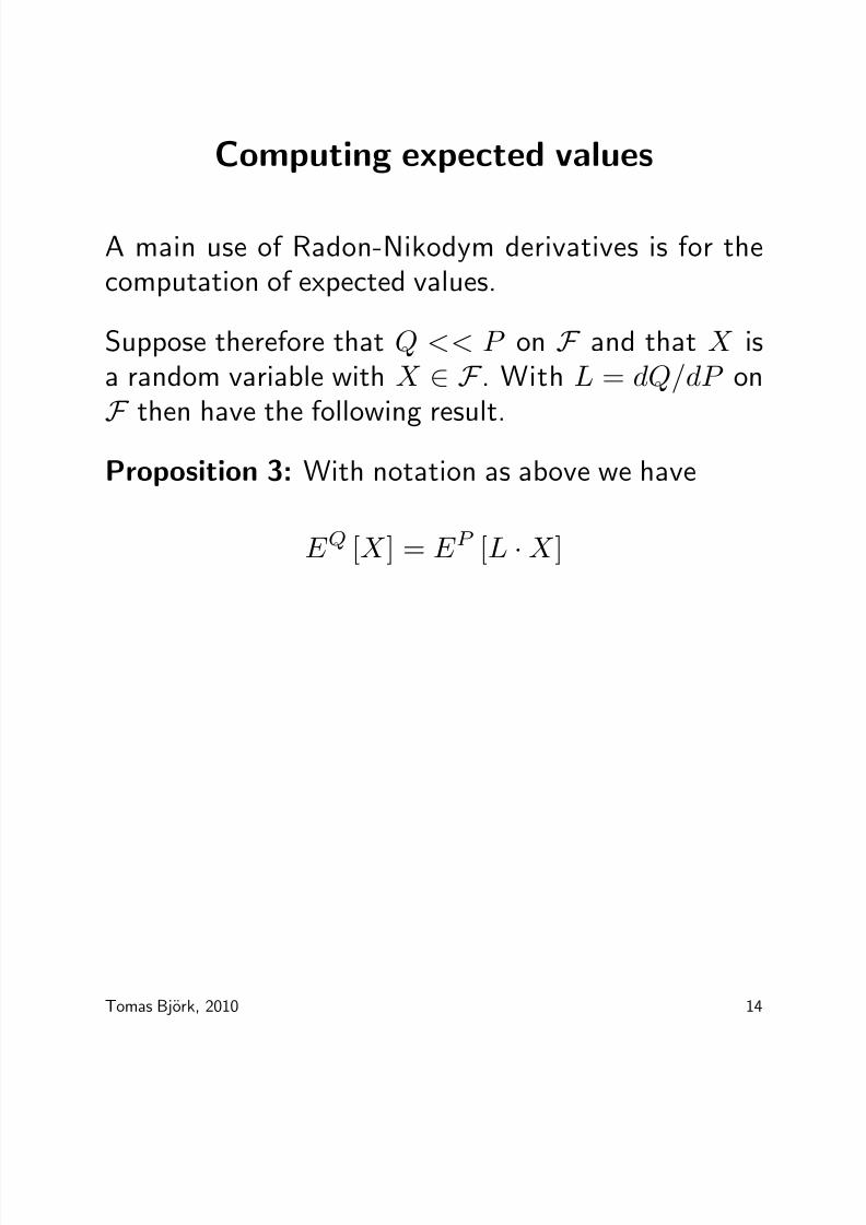
Computing expected values
A main use of Radon-Nikodym derivatives is for thecomputation of expected values.
Suppose therefore that Q << P on F and that X isa random variable with X ∈ F . With L = dQ/dP on
F then have the following result.
Proposition 3: With notation as above we have
E Q [X ] = E P [L · X ]
Tomas Bjork, 2010 14

8/13/2019 Bjork Notes
http://slidepdf.com/reader/full/bjork-notes 16/202
The Abstract Bayes’ Formula
We can also use Radon-Nikodym derivatives in order tocompute conditional expectations. The result, knownas the abstract Bayes’ Formula, is as follows.
Theorem 4: Consider two measures P and Q withQ << P on
F and with
LF = dQ
dP on F
Assume that G ⊆ F and let X be a random variablewith X
∈ F . Then the following holds
E Q [X | G] = E P
LF X
GE P [LF | G]
Tomas Bjork, 2010 15

8/13/2019 Bjork Notes
http://slidepdf.com/reader/full/bjork-notes 17/202
Dependence of the σ-algebra
Suppose that we have Q << P on F with
LF = dQ
dP on F
Now consider smaller σ-algebra G ⊆ F . Our problem
is to find the R-N derivative
LG = dQ
dP on G
We recall that LG is characterized by the following
properties
1. Q(A) = E P
LG · I A ∀A ∈ G
2. LG ≥ 0
3. E P
LG
= 1
4. LG ∈ G
Tomas Bjork, 2010 16

8/13/2019 Bjork Notes
http://slidepdf.com/reader/full/bjork-notes 18/202
A natural guess would perhaps be that LG = LF , solet us check if LF satisfies points 1-4 above.
By assumption we have
Q(A) = E P
LF · I A
∀A ∈ F
Since G ⊆ F we then have
Q(A) = E P
LF · I A ∀A ∈ G
so point 1 above is certainly satisfied by LF . It isalso clear that LF satisfies points 2 and 3. It thusseems that LF is also a natural candidate for the R-Nderivative LG, but the problem is that we do not ingeneral have LF ∈ G.
This problem can, however, be fixed. By iterated
expectations we have, for all A ∈ G,
E P
LF · I A
= E P
E P
LF · I AG
Tomas Bjork, 2010 17

8/13/2019 Bjork Notes
http://slidepdf.com/reader/full/bjork-notes 19/202
Since A ∈ G we have
E P
LF · I AG = E P
LF
G I A
Let us now define LG by
LG = E P LF
GWe then obviously have LG ∈ G and
Q(A) = E P
LG · I A ∀A ∈ G
It is easy to see that also points 2-3 are satisfied so we
have proved the following result.
Tomas Bjork, 2010 18

8/13/2019 Bjork Notes
http://slidepdf.com/reader/full/bjork-notes 20/202
A formula for LG
Proposition 5: If Q << P on F and G ⊆ F then,with notation as above, we have
LG = E P LF G
Tomas Bjork, 2010 19

8/13/2019 Bjork Notes
http://slidepdf.com/reader/full/bjork-notes 21/202
The likelihood process on a filtered space
We now consider the case when we have a probabilitymeasure P on some space Ω and that instead of justone σ-algebra F we have a filtration, i.e. an increasingfamily of σ-algebras F tt≥0.
The interpretation is as usual that F t is the informationavailable to us at time t, and that we have
F s ⊆ F tfor s ≤ t.
Now assume that we also have another measure Q,and that for some fixed T , we have Q << P on F T .We define the random variable LT by
LT = dQdP on F T
Since Q << P on F T we also have Q << P on F tfor all t ≤ T and we define
Lt = dQ
dP
on
F t 0
≤t
≤T
For every t we have Lt ∈ F t, so L is an adaptedprocess, known as the likelihood process.
Tomas Bjork, 2010 20

8/13/2019 Bjork Notes
http://slidepdf.com/reader/full/bjork-notes 22/202
The L process is a P martingale
We recall that
Lt = dQ
dP on F t 0 ≤ t ≤ T
Since F s ⊆ F t for s ≤ t we can use Proposition 5 anddeduce that
Ls = E P [Lt| F s] s ≤ t ≤ T
and we have thus proved the following result.
Proposition: Given the assumptions above, thelikelihood process L is a P -martingale.
Tomas Bjork, 2010 21

8/13/2019 Bjork Notes
http://slidepdf.com/reader/full/bjork-notes 23/202
Where are we heading?
We are now going to perform measure transformationson Wiener spaces, where P will correspond to theobjective measure and Q will be the risk neutralmeasure.
For this we need define the proper likelihood process Land, since L is a P -martingale, we have the followingnatural questions.
• What does a martingale look like in a Wiener drivenframework?
• Suppose that we have a P -Wiener process W andthen change measure from P to Q. What are theproperties of W under the new measure Q?
These questions are handled by the Martingale
Representation Theorem, and the Girsanov Theoremrespectively.
Tomas Bjork, 2010 22

8/13/2019 Bjork Notes
http://slidepdf.com/reader/full/bjork-notes 24/202
3.
The Martingale Representation Theorem
Tomas Bjork, 2010 23

8/13/2019 Bjork Notes
http://slidepdf.com/reader/full/bjork-notes 25/202
Intuition
Suppose that we have a Wiener process W underthe measure P . We recall that if h is adapted (andintegrable enough) and if the process X is defined by
X t = x
0 + t
0
hs
dW s
then X is a a martingale. We now have the followingnatural question:
Question: Assume that X is an arbitrary martingale.
Does it then follow that X has the form
X t = x0 +
t0
hsdW s
for some adapted process h?
In other words: Are all martingales stochastic integralsw.r.t. W ?
Tomas Bjork, 2010 24

8/13/2019 Bjork Notes
http://slidepdf.com/reader/full/bjork-notes 26/202
Answer
It is immediately clear that all martingales can not bewritten as stochastic integrals w.r.t. W . Consider forexample the process X defined by
X t =
0 for 0 ≤ t < 1Z for t ≥ 1
where Z is an random variable, independent of W ,with E [Z ] = 0.
X is then a martingale (why?) but it is clear (how?)that it cannot be written as
X t = x0 +
t0
hsdW s
for any process h.
Tomas Bjork, 2010 25

8/13/2019 Bjork Notes
http://slidepdf.com/reader/full/bjork-notes 27/202
Intuition
The intuitive reason why we cannot write
X t = x0 + t
0
hsdW s
in the example above is of course that the randomvariable Z “has nothing to do with” the Wiener processW . In order to exclude examples like this, we thus needan assumption which guarantees that our probabilityspace only contains the Wiener process W and nothing
else.
This idea is formalized by assuming that the filtrationF tt≥0 is the one generated by the Wienerprocess W .
Tomas Bjork, 2010 26

8/13/2019 Bjork Notes
http://slidepdf.com/reader/full/bjork-notes 28/202
The Martingale Representation Theorem
Theorem. Let W be a P -Wiener process and assumethat the filtation is the internal one i.e.
F t =
F W t = σ
W s; 0
≤s
≤t
Then, for every (P, F t)-martingale X , there exists areal number x and an adapted process h such that
X t = x + t
0
hsdW s,
i.e.dX t = htdW t.
Proof: Hard. This is very deep result.
Tomas Bjork, 2010 27

8/13/2019 Bjork Notes
http://slidepdf.com/reader/full/bjork-notes 29/202
Note
For a given martingale X , the Representation Theoremabove guarantees the existence of a process h such that
X t = x + t
0 hsdW s,
The Theorem does not, however, tell us how to findor construct the process h.
Tomas Bjork, 2010 28

8/13/2019 Bjork Notes
http://slidepdf.com/reader/full/bjork-notes 30/202
4.
The Girsanov Theorem
Tomas Bjork, 2010 29

8/13/2019 Bjork Notes
http://slidepdf.com/reader/full/bjork-notes 31/202
Setup
Let W be a P -Wiener process and fix a time horizonT . Suppose that we want to change measure from P to Q on F T . For this we need a P -martingale L withL0 = 1 to use as a likelihood process, and a naturalway of constructing this is to choose a process g andthen define L by
dLt = gtdW t
L0 = 1
This definition does not guarantee that L ≥ 0, so we
make a small adjustment. We choose a process ϕ anddefine L by
dLt = LtϕtdW t
L0 = 1
The process L will again be a martingale and we easilyobtain
Lt = eR t
0 ϕsdW s−12
R t0 ϕ
2sds
Tomas Bjork, 2010 30

8/13/2019 Bjork Notes
http://slidepdf.com/reader/full/bjork-notes 32/202
Thus we are guaranteed that L ≥
0. We now changemeasure form P to Q by setting
dQ = LtdP, on F t, 0 ≤ t ≤ T
The main problem is to find out what the propertiesof W are, under the new measure Q. This problem isresolved by the Girsanov Theorem.
Tomas Bjork, 2010 31

8/13/2019 Bjork Notes
http://slidepdf.com/reader/full/bjork-notes 33/202

8/13/2019 Bjork Notes
http://slidepdf.com/reader/full/bjork-notes 34/202
Changing the drift in an SDE
The single most common use of the Girsanov Theoremis as follows.
Suppose that we have a process X with P dynamics
dX t = µtdt + σtdW t
where µ and σ are adapted and W is P -Wiener.
We now do a Girsanov Transformation as above, andthe question is what the Q-dynamics look like.
From the Girsanov Theorem we have
dW t = ϕtdt + dW Qt
and substituting this into the P -dynamics we obtainthe Q dynamics as
dX t =
µt + σtϕt
dt + σtdW Q
t
Moral: The drift changes but the diffusion isunaffected.
Tomas Bjork, 2010 33

8/13/2019 Bjork Notes
http://slidepdf.com/reader/full/bjork-notes 35/202
The Converse of the Girsanov Theorem
Let W be a P -Wiener process. Fix a time horizon T .
Theorem. Assume that:
• Q << P on F T , with likelihood process
Lt = dQ
dP , on F t 0, ≤ t ≤ T
• The filtation is the internal one .i.e.
F t = σ W s; 0 ≤ s ≤ t
Then there exists a process ϕ such that
dLt = LtϕtdW t
L0 = 1
Tomas Bjork, 2010 34

8/13/2019 Bjork Notes
http://slidepdf.com/reader/full/bjork-notes 36/202
2.
The Martingale Approach
Ch. 10-12
Tomas Bjork, 2010 35

8/13/2019 Bjork Notes
http://slidepdf.com/reader/full/bjork-notes 37/202
Financial Markets
Price Processes:
S t =
S 0t ,...,S N t
Example: (Black-Scholes, S 0 := B, S 1 := S )
dS t = αS tdt + σS tdW t,
dBt = rBtdt.
Portfolio:ht = h0
t ,...,hN t
hit = number of units of asset i at time t.
Value Process:
V ht =N i=0
hitS it = htS t
Tomas Bjork, 2010 36

8/13/2019 Bjork Notes
http://slidepdf.com/reader/full/bjork-notes 38/202
Self Financing Portfolios
Definition: (intuitive)A portfolio is self-financing if there is no exogenousinfusion or withdrawal of money. “The purchase of anew asset must be financed by the sale of an old one.”
Definition: (mathematical)A portfolio is self-financing if the value processsatisfies
dV t =
N
i=0
hi
tdS i
t
Major insight:If the price process S is a martingale, and if h isself-financing, then V is a martingale.
NB! This simple observation is in fact the basis of thefollowing theory.
Tomas Bjork, 2010 37

8/13/2019 Bjork Notes
http://slidepdf.com/reader/full/bjork-notes 39/202
Arbitrage
The portfolio u is an arbitrage portfolio if
• The portfolio strategy is self financing.
• V 0 = 0.
• V T ≥ 0, P − a.s.
• P (V T > 0) > 0
Main Question: When is the market free of arbitrage?
Tomas Bjork, 2010 38

8/13/2019 Bjork Notes
http://slidepdf.com/reader/full/bjork-notes 40/202
First Attempt
Proposition: If S 0t , · · · , S N t are P -martingales, then
the market is free of arbitrage.
Proof:Assume that V is an arbitrage strategy. Since
dV t =N i=0
hitdS it,
V is a P -martingale, so
V 0 = E P [V T ] > 0.
This contradicts V 0 = 0.
True, but useless.
Tomas Bjork, 2010 39
8/13/2019 Bjork Notes
http://slidepdf.com/reader/full/bjork-notes 41/202
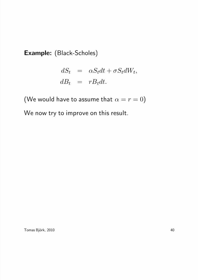
Example: (Black-Scholes)
dS t = αS tdt + σS tdW t,
dBt = rBtdt.
(We would have to assume that α = r = 0)
We now try to improve on this result.
Tomas Bjork, 2010 40

8/13/2019 Bjork Notes
http://slidepdf.com/reader/full/bjork-notes 42/202
Choose S0 as numeraire
Definition:The normalized price vector Z is given by
Z t =
S tS 0t =
1, Z
1t ,...,Z
N
t
The normalized value process V Z is given by
V Z
t
=N
0
hi
t
Z i
t
.
Idea:The arbitrage and self financing concepts should beindependent of the accounting unit.
Tomas Bjork, 2010 41

8/13/2019 Bjork Notes
http://slidepdf.com/reader/full/bjork-notes 43/202
Invariance of numeraire
Proposition: One can show (see the book) that
• S -arbitrage ⇐⇒ Z -arbitrage.
• S -self-financing ⇐⇒ Z -self-financing.
Insight:
• If h self-financing then
dV Z t =
N 1
hitdZ
it
• Thus, if the normalized price process Z is a P -martingale, then V Z is a martingale.
Tomas Bjork, 2010 42

8/13/2019 Bjork Notes
http://slidepdf.com/reader/full/bjork-notes 44/202
Second Attempt
Proposition: If Z 0t , · · · , Z N t are P -martingales, then
the market is free of arbitrage.
True, but still fairly useless.
Example: (Black-Scholes)
dS t = αS tdt + σS tdW t,
dBt = rBtdt.
dZ 1t = (α − r)Z 1t dt + σZ 1t dW t,
dZ 0t = 0dt.
We would have to assume “risk-neutrality”, i.e. thatα = r.
Tomas Bjork, 2010 43

8/13/2019 Bjork Notes
http://slidepdf.com/reader/full/bjork-notes 45/202
Arbitrage
Recall that h is an arbitrage if
• h is self financing
• V 0 = 0.
• V T ≥ 0, P − a.s.
• P (V T > 0) > 0
Major insight
This concept is invariant under an equivalent changeof measure!
Tomas Bjork, 2010 44

8/13/2019 Bjork Notes
http://slidepdf.com/reader/full/bjork-notes 46/202
Martingale Measures
Definition: A probability measure Q is called anequivalent martingale measure (EMM) if and onlyif it has the following properties.
• Q and P are equivalent, i.e.
Q ∼ P
• The normalized price processes
Z it = S itS 0t
, i = 0, . . . , N
are Q-martingales.
Wan now state the main result of arbitrage theory.
Tomas Bjork, 2010 45

8/13/2019 Bjork Notes
http://slidepdf.com/reader/full/bjork-notes 47/202
First Fundamental Theorem
Theorem: The market is arbitrage free
iff
there exists an equivalent martingale measure.
Tomas Bjork, 2010 46

8/13/2019 Bjork Notes
http://slidepdf.com/reader/full/bjork-notes 48/202
Comments
• It is very easy to prove that existence of EMMimples no arbitrage (see below).
• The other imnplication is technically very hard.
• For discrete time and finite sample space Ω the hardpart follows easily from the separation theorem forconvex sets.
• For discrete time and more general sample space weneed the Hahn-Banach Theorem.
• For continuous time the proof becomes technicallyvery hard, mainly due to topological problems. Seethe textbook.
Tomas Bjork, 2010 47

8/13/2019 Bjork Notes
http://slidepdf.com/reader/full/bjork-notes 49/202
Proof that EMM implies no arbitrage
This is basically done above. Assume that there existsan EMM denoted by Q. Assume that P (V T ≥ 0) = 1and P (V T > 0) > 0. Then, since P ∼ Q we also haveQ(V T ≥ 0) = 1 and Q(V T > 0) > 0.
Recall:
dV Z t =
N 1
hitdZ it
Q is a martingale measure
⇓
V Z is a Q-martingale
⇓
V 0 = V Z 0 = E Q
V Z T
> 0
⇓No arbitrage
Tomas Bjork, 2010 48

8/13/2019 Bjork Notes
http://slidepdf.com/reader/full/bjork-notes 50/202
Choice of Numeraire
The numeraire price S 0t can be chosen arbitrarily. Themost common choice is however that we choose S 0 asthe bank account, i.e.
S 0t = Bt
wheredBt = rtBtdt
Here r is the (possibly stochastic) short rate and we
have
Bt = eR t
0 rsds
Tomas Bjork, 2010 49

8/13/2019 Bjork Notes
http://slidepdf.com/reader/full/bjork-notes 51/202
Example: The Black-Scholes Model
dS t = αS tdt + σS tdW t,
dBt = rBtdt.
Look for martingale measure. We set Z = S/B.
dZ t = Z t(α − r)dt + Z tσdW t,
Girsanov transformation on [0, T ]:
dLt = LtϕtdW t,
L0 = 1.
dQ = LT dP, on F T Girsanov:
dW t = ϕtdt + dW Qt ,
where W Q is a Q-Wiener process.
Tomas Bjork, 2010 50

8/13/2019 Bjork Notes
http://slidepdf.com/reader/full/bjork-notes 52/202
The Q-dynamics for Z are given by
dZ t = Z t [α − r + σϕt] dt + Z tσdW Qt .
Unique martingale measure Q, with Girsanov kernel
given byϕt =
r − α
σ .
Q-dynamics of S :
dS t = rS tdt + σS tdW Qt .
Conclusion: The Black-Scholes model is free of arbitrage.
Tomas Bjork, 2010 51

8/13/2019 Bjork Notes
http://slidepdf.com/reader/full/bjork-notes 53/202
Pricing
We consider a market Bt, S 1t , . . . , S N t .
Definition:A contingent claim with delivery time T , is a randomvariable
X ∈ F
T .
“At t = T the amount X is paid to the holder of theclaim”.
Example: (European Call Option)
X = max [S T − K, 0]
Let X be a contingent T -claim.
Problem: How do we find an arbitrage free priceprocess Πt [X ] for X ?
Tomas Bjork, 2010 52

8/13/2019 Bjork Notes
http://slidepdf.com/reader/full/bjork-notes 54/202
Solution
The extended market
Bt, S 1t , . . . , S N t , Πt [X ]
must be arbitrage free, so there must exist a martingale
measure Q for (Bt, S t, Πt [X ]). In particular
Πt [X ]
Bt
must be a Q-martingale, i.e.
Πt [X ]
Bt
= E Q
ΠT [X ]
BT
F t
Since we obviously (why?) have
ΠT [X ] = X
we have proved the main pricing formula.
Tomas Bjork, 2010 53

8/13/2019 Bjork Notes
http://slidepdf.com/reader/full/bjork-notes 55/202
Risk Neutral Valuation
Theorem: For a T -claim X , the arbitrage free price isgiven by the formula
Πt [X ] = E
Q e
−R T t rsds
× X F t
Tomas Bjork, 2010 54

8/13/2019 Bjork Notes
http://slidepdf.com/reader/full/bjork-notes 56/202

8/13/2019 Bjork Notes
http://slidepdf.com/reader/full/bjork-notes 57/202
Problem
Recall the valuation formula
Πt [X ] = E Q e−R T t rsds × X F t
What if there are several different martingale measuresQ?
This is connected with the completeness of themarket.
Tomas Bjork, 2010 56

8/13/2019 Bjork Notes
http://slidepdf.com/reader/full/bjork-notes 58/202
Hedging
Def: A portfolio is a hedge against X (“replicatesX ”) if
• h is self financing
• V T = X, P − a.s.
Def: The market is complete if every X can behedged.
Pricing Formula:If h replicates X , then a natural way of pricing X is
Πt [X ] = V ht
When can we hedge?
Tomas Bjork, 2010 57

8/13/2019 Bjork Notes
http://slidepdf.com/reader/full/bjork-notes 59/202
Existence of hedge
Existence of stochastic integralrepresentation
Tomas Bjork, 2010 58

8/13/2019 Bjork Notes
http://slidepdf.com/reader/full/bjork-notes 60/202
Fix T -claim X .
If h is a hedge for X then
• V Z T = XBT
• h is self financing, i.e.
dV Z t =K 1
hitdZ it
Thus V Z is a Q-martingale.
V Z t = E Q
X
BT
F t
Tomas Bjork, 2010 59

8/13/2019 Bjork Notes
http://slidepdf.com/reader/full/bjork-notes 61/202
Lemma:Fix T -claim X . Define martingale M by
M t = E Q
X
Bt
F t
Suppose that there exist predictable processesh1, · · · , hN such that
M t = x +N
i=1
t
0
hisdZ is,
Then X can be replicated.
Tomas Bjork, 2010 60

8/13/2019 Bjork Notes
http://slidepdf.com/reader/full/bjork-notes 62/202
Proof
We guess that
M t = V Z t = hBt · 1 +
N i=1
hitZ it
Define: hB
by
hBt = M t −
N i=1
hitZ it.
We have M t = V
Z
t , and we get
dV Z t = dM t =N i=1
hitdZti,
so the portfolio is self financing. Furthermore:
V Z T = M T = E Q
X
BT
F T
= X
BT
.
Tomas Bjork, 2010 61
8/13/2019 Bjork Notes
http://slidepdf.com/reader/full/bjork-notes 63/202
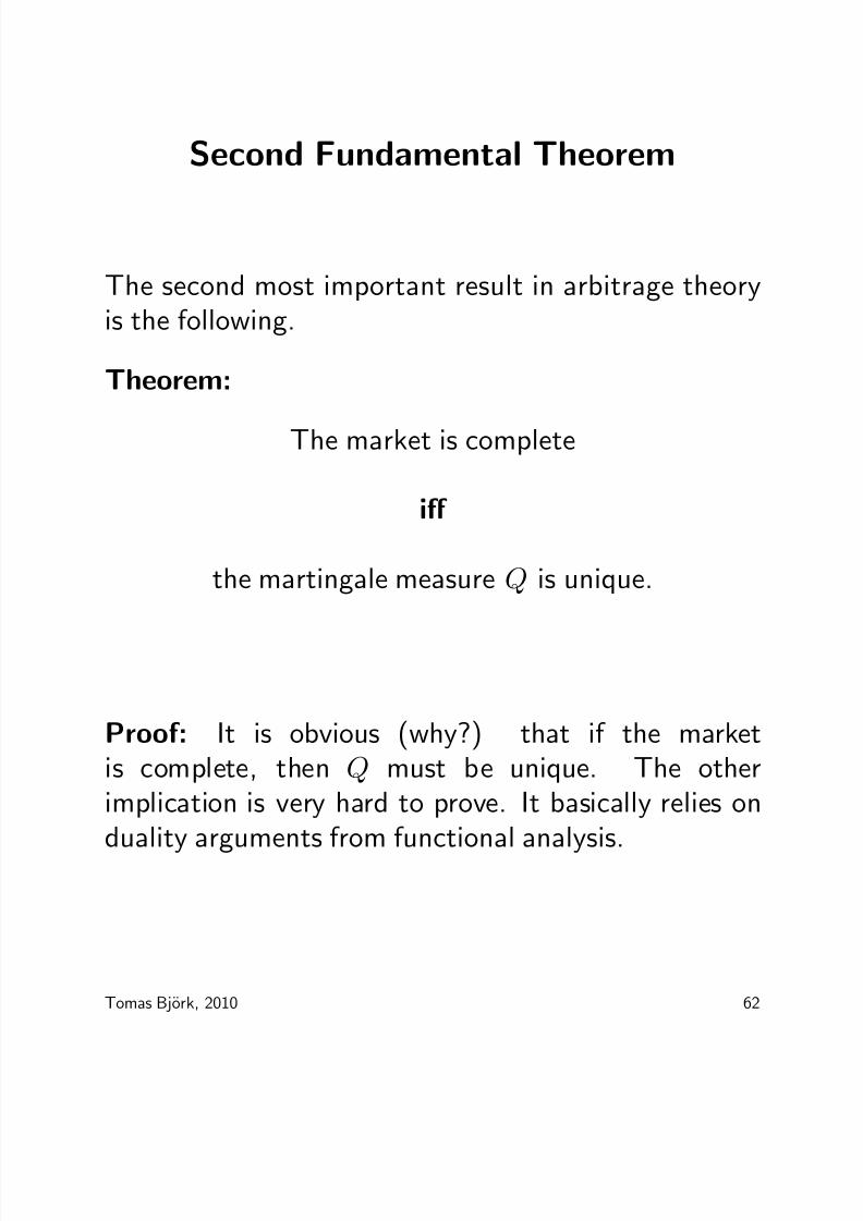
Second Fundamental Theorem
The second most important result in arbitrage theoryis the following.
Theorem:
The market is complete
iff
the martingale measure Q is unique.
Proof: It is obvious (why?) that if the marketis complete, then Q must be unique. The otherimplication is very hard to prove. It basically relies onduality arguments from functional analysis.
Tomas Bjork, 2010 62

8/13/2019 Bjork Notes
http://slidepdf.com/reader/full/bjork-notes 64/202
Black-Scholes Model
Q-dynamics
dS t = rS tdt + σS tdW Qt ,
dZ t = Z tσdW Qt
M t = E Q
e−rT X F t
,
Representation theorem for Wiener processes
⇓there exists g such that
M t = M (0) +
t0
gsdW Qs .
Thus
M t = M 0 + t
0h1sdZ s,
with h1t = gt
σZ t.
Tomas Bjork, 2010 63

8/13/2019 Bjork Notes
http://slidepdf.com/reader/full/bjork-notes 65/202
Result:X can be replicated using the portfolio defined by
h1t = gt/σZ t,
hBt = M t − h1
tZ t.
Moral: The Black Scholes model is complete.
Tomas Bjork, 2010 64

8/13/2019 Bjork Notes
http://slidepdf.com/reader/full/bjork-notes 66/202
Special Case: Simple Claims
Assume X is of the form X = Φ(S T )
M t = E Q
e−rT Φ(S T )F t
,
Kolmogorov backward equation ⇒ M t = f (t, S t)
∂f
∂t + rs∂f
∂s + 1
2σ2
s2∂
2f
∂s2 = 0,f (T, s) = e−rT Φ(s).
Ito ⇒dM t = σS t
∂f
∂sdW Qt ,
so
gt = σS t · ∂f ∂s
,
Replicating portfolio h:
hBt = f − S t
∂f
∂s,
h1t = Bt
∂f
∂s .
Interpretation: f (t, S t) = V Z t .
Tomas Bjork, 2010 65

8/13/2019 Bjork Notes
http://slidepdf.com/reader/full/bjork-notes 67/202
Define F (t, s) by
F (t, s) = ertf (t, s)
so F (t, S t) = V t. Then
hB
t = F (t,S t)−S t
∂F ∂s
(t,S t)
Bt,
h1t = ∂F
∂s(t, S t)
where F solves the Black-Scholes equation
∂F ∂t
+ rs∂F ∂s
+ 12σ2s2∂ 2F
∂s2 − rF = 0,F (T, s) = Φ(s).
Tomas Bjork, 2010 66

8/13/2019 Bjork Notes
http://slidepdf.com/reader/full/bjork-notes 68/202
Main Results
• The market is arbitrage free ⇔ There exists amartingale measure Q
• The market is complete ⇔ Q is unique.
• Every X must be priced by the formula
Πt [X ] = E Q
e−R T t rsds × X
F t
for some choice of Q.
• In a non-complete market, different choices of Qwill produce different prices for X .
• For a hedgeable claim X, all choices of Q willproduce the same price for X:
Πt [X ] = V t = E Q
e−R T t rsds × X
F t
Tomas Bjork, 2010 67

8/13/2019 Bjork Notes
http://slidepdf.com/reader/full/bjork-notes 69/202
Completeness vs No Arbitrage
Rule of Thumb
Question:When is a model arbitrage free and/or complete?
Answer:Count the number of risky assets, and the number of random sources.
R = number of random sources
N = number of risky assets
Intuition:If N is large, compared to R, you have lots of possibilities of forming clever portfolios. Thus lotsof chances of making arbitrage profits. Also many
chances of replicating a given claim.
Tomas Bjork, 2010 68

8/13/2019 Bjork Notes
http://slidepdf.com/reader/full/bjork-notes 70/202
Rule of thumb
Generically, the following hold.
• The market is arbitrage free if and only if
N ≤ R
• The market is complete if and only if
N ≥ R
Example:The Black-Scholes model.
dS t = αS tdt + σS tdW t,
dBt = rBtdt.
For B-S we have N = R = 1. Thus the Black-Scholesmodel is arbitrage free and complete.
Tomas Bjork, 2010 69

8/13/2019 Bjork Notes
http://slidepdf.com/reader/full/bjork-notes 71/202
Stochastic Discount Factors
Given a model under P . For every EMM Q we definethe corresponding Stochastic Discount Factor, orSDF, by
Dt = e−R t
0 rsdsLt,
whereLt =
dQ
dP , on F t
There is thus a one-to-one correspondence betweenEMMs and SDFs.
The risk neutral valuation formula for a T -claim X cannow be expressed under P instead of under Q.
Proposition: With notation as above we have
Πt [X ] = 1
Dt
E P [DT X
| F t]
Proof: Bayes’ formula.
Tomas Bjork, 2010 70

8/13/2019 Bjork Notes
http://slidepdf.com/reader/full/bjork-notes 72/202

8/13/2019 Bjork Notes
http://slidepdf.com/reader/full/bjork-notes 73/202
3.
Incomplete Markets
Ch. 15
Tomas Bjork, 2010 72

8/13/2019 Bjork Notes
http://slidepdf.com/reader/full/bjork-notes 74/202
Derivatives on Non Financial Underlying
Recall: The Black-Scholes theory assumes that themarket for the underlying asset has (among otherthings) the following properties.
• The underlying is a liquidly traded asset.
• Shortselling allowed.
• Portfolios can be carried forward in time.
There exists a large market for derivatives, where the
underlying does not satisfy these assumptions.
Examples:
• Weather derivatives.
• Derivatives on electric energy.
• CAT-bonds.
Tomas Bjork, 2010 73

8/13/2019 Bjork Notes
http://slidepdf.com/reader/full/bjork-notes 75/202
Typical Contracts
Weather derivatives:“Heating degree days”. Payoff at maturity T isgiven by
Z = max X T − 30, 0
where X T is the (mean) temperature at some place.
Electricity option:The right (but not the obligation) to buy, at timeT , at a predetermined price K , a constant flow of energy over a predetermined time interval.
CAT bond:A bond for which the payment of coupons andnominal value is contingent on some (well specified)natural disaster to take place.
Tomas Bjork, 2010 74

8/13/2019 Bjork Notes
http://slidepdf.com/reader/full/bjork-notes 76/202
Problems
Weather derivatives:The temperature is not the price of a traded asset.
Electricity derivatives:
Electric energy cannot easily be stored.
CAT-bonds:Natural disasters are not traded assets.
We will treat all these problems within a factor model.
Tomas Bjork, 2010 75

8/13/2019 Bjork Notes
http://slidepdf.com/reader/full/bjork-notes 77/202
Typical Factor Model Setup
Given:
• An underlying factor process X , which is not theprice process of a traded asset, with dynamics under
the objective probability measure P as
dX t = µ (t, X t) dt + σ (t, X t) dW t.
• A risk free asset with dynamics
dBt = rBtdt,
Problem:Find arbitrage free price Πt [Z ] of a derivative of the
form Z = Φ(X T )
Tomas Bjork, 2010 76

8/13/2019 Bjork Notes
http://slidepdf.com/reader/full/bjork-notes 78/202
Concrete Examples
Assume that X t is the temperature at time t at thevillage of Peniche (Portugal).
Heating degree days:
Φ(X T ) = 100 · max X T − 30, 0
Holiday Insurance:
Φ(X T ) =
1000, if X T < 20
0, if X T ≥ 20
Tomas Bjork, 2010 77

8/13/2019 Bjork Notes
http://slidepdf.com/reader/full/bjork-notes 79/202
Question
Is the price Πt [Φ] uniquely determined by the P -dynamics of X , and the requirement of an arbitragefree derivatives market?
Tomas Bjork, 2010 78

8/13/2019 Bjork Notes
http://slidepdf.com/reader/full/bjork-notes 80/202
NO!!
WHY?
Tomas Bjork, 2010 79

8/13/2019 Bjork Notes
http://slidepdf.com/reader/full/bjork-notes 81/202
Stock Price Model ∼ Factor Model
Black-Scholes:
dS t = µS tdt + σS tdW t,
dBt = rBtdt.
Factor Model:
dX t = µ(t, X t)dt + σ(t, X t)dW t,
dBt = rBtdt.
What is the difference?
Tomas Bjork, 2010 80

8/13/2019 Bjork Notes
http://slidepdf.com/reader/full/bjork-notes 82/202
Answer
• X is not the price of a traded asset!
• We can not form a portfolio based on X .
Tomas Bjork, 2010 81

8/13/2019 Bjork Notes
http://slidepdf.com/reader/full/bjork-notes 83/202
1. Rule of thumb:
N = 0, (no risky asset)R = 1, (one source of randomness, W )
We have N < R. The exogenously given market,consisting only of B, is incomplete.
2. Replicating portfolios:We can only invest money in the bank, and then sitdown passively and wait.
We do not have enough underlying assets in orderto price X -derivatives.
Tomas Bjork, 2010 82
8/13/2019 Bjork Notes
http://slidepdf.com/reader/full/bjork-notes 84/202
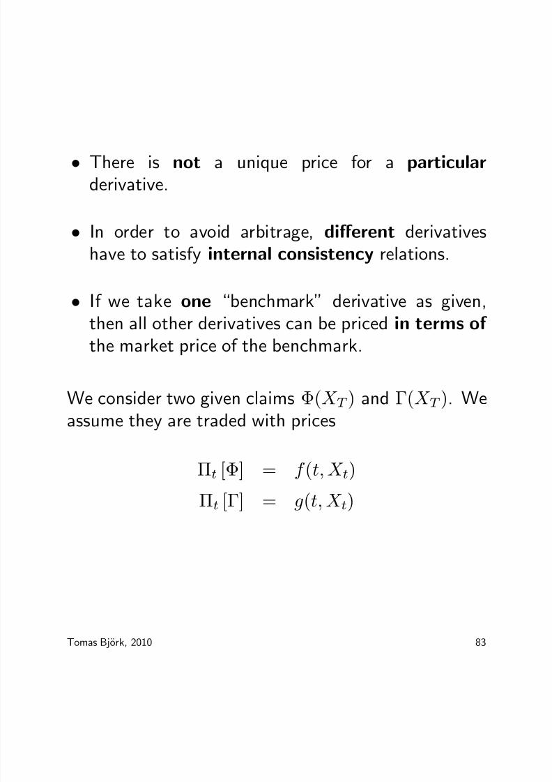
• There is not a unique price for a particularderivative.
• In order to avoid arbitrage, different derivativeshave to satisfy internal consistency relations.
• If we take one “benchmark” derivative as given,then all other derivatives can be priced in terms of the market price of the benchmark.
We consider two given claims Φ(X T ) and Γ(X T ). Weassume they are traded with prices
Πt [Φ] = f (t, X t)
Πt [Γ] = g(t, X t)
Tomas Bjork, 2010 83

8/13/2019 Bjork Notes
http://slidepdf.com/reader/full/bjork-notes 85/202
Program:
• Form portfolio based on Φ and Γ. Use Ito on f andg to get portfolio dynamics.
dV = V
uf df
f + ugdg
g
• Choose portfolio weights such that the dW − termvanishes. Then we have
dV = V
·kdt,
(“synthetic bank” with k as the short rate)
• Absence of arbitrage implies
k = r
• Read off the relation k = r!
Tomas Bjork, 2010 84

8/13/2019 Bjork Notes
http://slidepdf.com/reader/full/bjork-notes 86/202
From Ito:df = f µf dt + f σf dW,
where µf =
f t+µf x+12σ
2f xxf
,
σf = σf xf
.
Portfolio dynamics
dV = V
uf df
f + ugdg
g
.
Reshuffling terms gives us
dV = V · uf µf + ugµg
dt + V · uf σf + ugσg
dW.
Let the portfolio weights solve the system
uf + ug = 1,
uf σf + ugσg = 0.
Tomas Bjork, 2010 85

8/13/2019 Bjork Notes
http://slidepdf.com/reader/full/bjork-notes 87/202
uf = −
σg
σf − σg
,
ug = σf
σf − σg
,
Portfolio dynamics
dV = V · uf µf + ugµg
dt.
i.e.
dV = V ·µgσf − µf σg
σf
−σg dt.
Absence of arbitrage requires
µgσf − µf σg
σf − σg
= r
which can be written asµg − r
σg
= µf − r
σf
.
Tomas Bjork, 2010 86

8/13/2019 Bjork Notes
http://slidepdf.com/reader/full/bjork-notes 88/202
µg − r
σg
= µf − r
σf
.
Note!The quotient does not depend upon the particular
choice of contract.
Tomas Bjork, 2010 87

8/13/2019 Bjork Notes
http://slidepdf.com/reader/full/bjork-notes 89/202
Result
Assume that the market for X -derivatives is free of arbitrage. Then there exists a universal process λ,such that
µf (t) − r
σf (t) = λ(t, X t),
holds for all t and for every choice of contract f .
NB: The same λ for all choices of f .
λ = Risk premium per unit of volatility= “Market Price of Risk” (cf. CAPM).= Sharpe Ratio
Slogan:“On an arbitrage free market all X -derivatives havethe same market price of risk.”
The relationµf − r
σf
= λ
is actually a PDE!
Tomas Bjork, 2010 88

8/13/2019 Bjork Notes
http://slidepdf.com/reader/full/bjork-notes 90/202
Pricing Equation
f t + µ − λσ f x + 1
2σ2f xx − rf = 0
f (T, x) = Φ(x),
P -dynamics:
dX = µ(t, X )dt + σ(t, X )dW.
Can we solve the PDE?
Tomas Bjork, 2010 89

8/13/2019 Bjork Notes
http://slidepdf.com/reader/full/bjork-notes 91/202
No!!
Why??
Tomas Bjork, 2010 90

8/13/2019 Bjork Notes
http://slidepdf.com/reader/full/bjork-notes 92/202
Answer
Recall the PDE
f t + µ − λσ f x + 1
2σ2f xx − rf = 0
f (T, x) = Φ(x),
• In order to solve the PDE we need to know λ.
• λ is not given exogenously.
• λ is not determined endogenously.
Tomas Bjork, 2010 91

8/13/2019 Bjork Notes
http://slidepdf.com/reader/full/bjork-notes 93/202
Question:
Who determines λ?
Tomas Bjork, 2010 92

8/13/2019 Bjork Notes
http://slidepdf.com/reader/full/bjork-notes 94/202
Answer:
THE MARKET!
Tomas Bjork, 2010 93

8/13/2019 Bjork Notes
http://slidepdf.com/reader/full/bjork-notes 95/202
Interpreting λ
Recall that the f dynamics are
df = f µf dt + f σf dW t
and λ is defined as
µf (t) − rσf (t)
= λ(t, X t),
• λ measures the aggregate risk aversion in the
market.
• If λ is big then the market is highly risk averse.
• If λ is zero then the market is risk netural.
• If you make an assumption about λ, then youimplicitly make an assumption about the aggregaterisk aversion of the market.
Tomas Bjork, 2010 94

8/13/2019 Bjork Notes
http://slidepdf.com/reader/full/bjork-notes 96/202
Moral
• Since the market is incomplete the requirement of an arbitrage free market will not lead to uniqueprices for X -derivatives.
• Prices on derivatives are determined by two mainfactors.
1. Partly by the requirement of an arbitrage freederivative market. All pricing functions satisfiesthe same PDE.
2. Partly by supply and demand on the market.These are in turn determined by attitude towardsrisk, liquidity consideration and other factors. Allthese are aggregated into the particular λ used(implicitly) by the market.
Tomas Bjork, 2010 95

8/13/2019 Bjork Notes
http://slidepdf.com/reader/full/bjork-notes 97/202
Risk Neutral Valuation
We recall the PDE
f t + µ − λσ f x + 1
2σ2f xx − rf = 0
f (T, x) = Φ(x),
Using Feynman-Kac we obtain a risk neutral valuationformula.
Tomas Bjork, 2010 96

8/13/2019 Bjork Notes
http://slidepdf.com/reader/full/bjork-notes 98/202
Risk Neutral Valuation
f (t, x) = e−r(T −t)E Qt,x [Φ(X T )]
Q-dynamics:
dX t = µ − λσ dt + σdW Qt
• Price = expected value of future payments
• The expectation should not be taken under the“objective” probabilities P , but under the “riskadjusted” probabilities Q.
Tomas Bjork, 2010 97

8/13/2019 Bjork Notes
http://slidepdf.com/reader/full/bjork-notes 99/202
Interpretation of the risk adjusted
probabilities
• The risk adjusted probabilities can be interpreted asprobabilities in a (fictuous) risk neutral world.
• When we compute prices, we can calculate as if we live in a risk neutral world.
• This does not mean that we live in, or think thatwe live in, a risk neutral world.
• The formulas above hold regardless of the attitudetowards risk of the investor, as long as he/she prefersmore to less.
Tomas Bjork, 2010 98

8/13/2019 Bjork Notes
http://slidepdf.com/reader/full/bjork-notes 100/202
Diversification argument about λ
• If the risk factor is idiosyncratic and diversifiable,then one can argue that the factor should not bepriced by the market. Compare with APT.
• Mathematically this means that λ = 0, i.e. P = Q,i.e. the risk neutral distribution coincides withthe objective distribution.
• We thus have the “actuarial pricing formula”
f (t, x) = e−r(T −t)
E P
t,x [Φ(X T )]
where we use the objective probabiliy measure P .
Tomas Bjork, 2010 99

8/13/2019 Bjork Notes
http://slidepdf.com/reader/full/bjork-notes 101/202
Modeling Issues
Temperature:A standard model is given by
dX t = m(t) − bX t dt + σdW t,
where m is the mean temperature capturingseasonal variations. This often works reasonably
well.
Electricity:A (naive) model for the spot electricity price is
dS t = S t
m(t)
−a ln S t
dt + σS tdW t
This implies lognormal prices (why?). Electrictyprices are however very far from lognormal, becauseof “spikes” in the prices. Complicated.
CAT bonds:
Here we have to use the theory of point processesand the theory of extremal statistics to modelnatural disasters. Complicated.
Tomas Bjork, 2010 100
8/13/2019 Bjork Notes
http://slidepdf.com/reader/full/bjork-notes 102/202
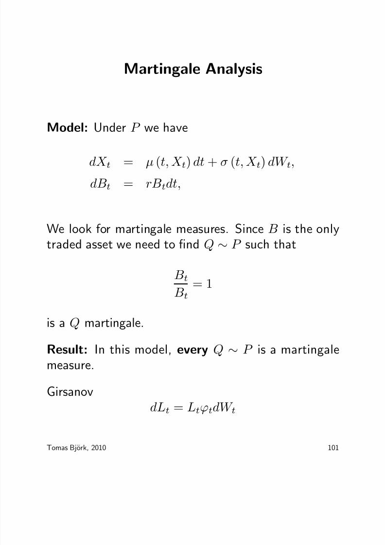
Martingale Analysis
Model: Under P we have
dX t = µ (t, X t) dt + σ (t, X t) dW t,
dBt
= rBtdt,
We look for martingale measures. Since B is the onlytraded asset we need to find Q ∼ P such that
Bt
Bt = 1
is a Q martingale.
Result: In this model, every Q ∼ P is a martingalemeasure.
GirsanovdLt = LtϕtdW t
Tomas Bjork, 2010 101

8/13/2019 Bjork Notes
http://slidepdf.com/reader/full/bjork-notes 103/202
P -dynamics
dX t = µ (t, X t) dt + σ (t, X t) dW t,
dLt = LtϕtdW t
dQ = LtdP on F tGirsanov:
dW t = ϕtdt + dW Qt
Martingale pricing:
F (t, x) = e−r(T −t)E Q [Z | F t]
Q-dynamics of X :
dX t = µ (t, X t) + σ (t, X t) ϕt dt + σ (t, X t) dW Qt ,
Result: We have λt = −ϕt, i.e,. the Girsanov kernelϕ equals minus the market price of risk.
Tomas Bjork, 2010 102

8/13/2019 Bjork Notes
http://slidepdf.com/reader/full/bjork-notes 104/202
Several Risk Factors
We recall the dynamics of the f -derivative
df = f µf dt + f σf dW t
and the Market Price of Risk
µf − r
σf
= λ, i.e. µf − r = λσf .
In a multifactor model of the type
dX t = µ (t, X t) dt +
ni=1
σi (t, X t) dW it ,
it follows from Girsanov that for every risk factor W i
there will exist a market price of risk λi = −ϕi suchthat
µf − r =
ni=1
λiσi
Compare with CAPM.
Tomas Bjork, 2010 103

8/13/2019 Bjork Notes
http://slidepdf.com/reader/full/bjork-notes 105/202
4.
Bonds and Interest Rates.
Short Rate Models
Ch. 22-23
Tomas Bjork, 2010 104

8/13/2019 Bjork Notes
http://slidepdf.com/reader/full/bjork-notes 106/202
Definitions
Bonds:T -bond = zero coupon bond, paying $1 at the date of maturity T .
p(t, T ) = price, at t, of a T -bond.
p(T, T ) = 1.
Main Problem
• Investigate the term structure, i.e. how prices of bonds with different dates of maturity are relatedto each other.
• Compute arbitrage free prices of interest ratederivatives (bond options, swaps, caps, floors etc.)
Tomas Bjork, 2010 105

8/13/2019 Bjork Notes
http://slidepdf.com/reader/full/bjork-notes 107/202
Risk Free Interest Rates
At time t:
• Sell one S -bond
• Buy exactly p(t, S )/p(t, T ) T
−bonds
• Net investment at t: $0.
At time S:
• Pay $1
At time T:
• Collect $ p(t, S )/p(t, T ) · 1
Tomas Bjork, 2010 106

8/13/2019 Bjork Notes
http://slidepdf.com/reader/full/bjork-notes 108/202
Net Effect
• The contract is made at t.
• An investment of 1 at time S has yielded p(t, S )/p(t, T ) at time T .
• The equivalent constant rates, R, are given as thesolutions to
Continuous rate:
eR·(T −S ) · 1 = p(t, S )
p(t, T )
Simple rate:
[1 + R · (T − S )] · 1 = p(t, S ) p(t, T )
Tomas Bjork, 2010 107

8/13/2019 Bjork Notes
http://slidepdf.com/reader/full/bjork-notes 109/202
Continuous Interest Rates
1. The forward rate for the period [S, T ],contracted at t is defined by
R(t; S, T ) = −log p(t, T ) − log p(t, S )
T −
S .
2. The spot rate, R(S, T ), for the period [S, T ] isdefined by
R(S, T ) = R(S ; S, T ).
3. The instantaneous forward rate at T , conractedat t is defined by
f (t, T ) = −∂ log p(t, T )
∂T = lim
S →T R(t; S, T ).
4. The instantaneous short rate at t is defined by
r(t) = f (t, t).
Tomas Bjork, 2010 108

8/13/2019 Bjork Notes
http://slidepdf.com/reader/full/bjork-notes 110/202
Simple Rates (LIBOR)
1. The simple forward rate L(t;S,T)for the period[S, T ], contracted at t is defined by
L(t; S, T ) = 1T − S
· p(t, S ) − p(t, T ) p(t, T )
2. The simple spot rate, L(S, T ), for the period[S, T ] is defined by
L(S, T ) = 1
T − S · 1 − p(S, T )
p(S, T )
Tomas Bjork, 2010 109

8/13/2019 Bjork Notes
http://slidepdf.com/reader/full/bjork-notes 111/202
Practical Formula (LIBOR)
The simple spot rate, L(T, T + δ ), for the period[T, T + δ ] is given by
p(T, T + δ ) =
1
1 + δL(T, T + δ )
i.e.
L = 1
δ · 1 − p
p
Tomas Bjork, 2010 110

8/13/2019 Bjork Notes
http://slidepdf.com/reader/full/bjork-notes 112/202
Bond prices ∼ forward rates
p(t, T ) = p(t, s) · exp
− T s
f (t, u)du
,
In particular we have
p(t, T ) = exp
− T t
f (t, s)ds
.
Tomas Bjork, 2010 111

8/13/2019 Bjork Notes
http://slidepdf.com/reader/full/bjork-notes 113/202
Interest Rate Options
Problem:We want to price, at t, a European Call, with exercisedate S , and strike price K , on an underlying T -bond.(t < S < T ).
Naive approach: Use Black-Scholes’s formula.
F (t, p) = pN [d1] − e−r(S −t)KN [d2] .
d1 = 1σ√
S − t
ln
pK
+
r + 12
σ2
(S − t)
,
d2 = d1 − σ√
S − t.
where
p = p(t, T )
Tomas Bjork, 2010 112

8/13/2019 Bjork Notes
http://slidepdf.com/reader/full/bjork-notes 114/202
Is this allowed?
• p shall be the price of a traded asset. OK!
• The volatility of p must be constant. Here we have
a problem because of pull-to-par, i.e. the fact that p(T, T ) = 1. Bond volatilities will tend to zero asthe bond approaches the time of maturity.
• The short rate must be constant anddeterministic. Here the approach collapses
completely, since the whole point of studyingbond prices lies in the fact that interest rates arestochastic.
There is some hope in the case when the remainingtime to exercise the option is small in relation to the
remaining time to maturity of the underlying bond(why?).
Tomas Bjork, 2010 113

8/13/2019 Bjork Notes
http://slidepdf.com/reader/full/bjork-notes 115/202
Deeply felt need
A consistent arbitrage free model for thebond market
Tomas Bjork, 2010 114

8/13/2019 Bjork Notes
http://slidepdf.com/reader/full/bjork-notes 116/202
Stochastic interest rates
We assume that the short rate r is a stochastic process.
Money in the bank will then grow according to:
dB(t) = r(t)B(t)dt,B(0) = 1.
i.e.
B(t) = eR t
0 r(s)ds
Tomas Bjork, 2010 115

8/13/2019 Bjork Notes
http://slidepdf.com/reader/full/bjork-notes 117/202
Models for the short rate
Model: (In reality)
P:
dr = µ(t, r)dt + σ(t, r)dW,
dB = r(t)Bdt.
Question: Are bond prices uniquely determinedby the P -dynamics of r, and the requirement of anarbitrage free bond market?
Tomas Bjork, 2010 116

8/13/2019 Bjork Notes
http://slidepdf.com/reader/full/bjork-notes 118/202
NO!!
WHY?
Tomas Bjork, 2010 117

8/13/2019 Bjork Notes
http://slidepdf.com/reader/full/bjork-notes 119/202
Stock Models ∼ Interest Rates
Black-Scholes:
dS = αSdt + σSdw,
dB = rBdt.
Interest Rates:
dr = µ(t, r)dt + σ(t, r)dW,
dB = rtBdt.
Question: What is the difference?
Answer: The short rate r is not the price of atraded asset!
Tomas Bjork, 2010 118

8/13/2019 Bjork Notes
http://slidepdf.com/reader/full/bjork-notes 120/202
1. Meta-Theorem:
N = 0, (no risky asset)R = 1, (one source of randomness, W )
We have M < R. The exongenously given market,consisting only of B, is incomplete.
2. Replicating portfolios:We can only invest money in the bank, and then sitdown passively and wait.
We do not have enough underlying assets in orderto price bonds.
Tomas Bjork, 2010 119

8/13/2019 Bjork Notes
http://slidepdf.com/reader/full/bjork-notes 121/202
• There is not a unique price for a particularT −bond.
• In order to avoid arbitrage, bonds of differentmaturities have to satisfy internal consistency
relations.
• If we take one “benchmark” T 0-bond as given, thenall other bonds can be priced in terms of the marketprice of the benchmark bond.
Assumption:
p(t, T ) = F (t, rt; T )
p(t, T ) = F T (t, rt),
F T (T, r) = 1.
Tomas Bjork, 2010 120

8/13/2019 Bjork Notes
http://slidepdf.com/reader/full/bjork-notes 122/202
Program
• Form portfolio based on T − and S −bonds. Use Itoon F T (t, r(t)) to get bond- and portfolio dynamics.
dV = V
uT dF T
F T + uS dF
S
F S
• Choose portfolio weights such that the dW − termvanishes. Then we have
dV = V · kdt,
(“synthetic bank” with k as the short rate)
• Absence of arbitrage ⇒ k = r .
• Read off the relation k = r!
Tomas Bjork, 2010 121

8/13/2019 Bjork Notes
http://slidepdf.com/reader/full/bjork-notes 123/202
From Ito:
dF T = F T αT dt + F T σT d W ,
where
αT = F T t +µF T r +1
2σ2F T rr
F T ,
σT = σF
T
rF T .
Portfolio dynamics
dV = V
uT dF T
F T + uS dF S
F S
.
Reshuffling terms gives us
dV = V ·uT αT + uS αS
dt+V ·uT σT + uS σS
dW.
Let the portfolio weights solve the system uT + uS = 1,
uT σT + uS σS = 0.
Tomas Bjork, 2010 122

8/13/2019 Bjork Notes
http://slidepdf.com/reader/full/bjork-notes 124/202
uT = − σS
σT −σS ,
uS = σT σT −σS
,
Portfolio dynamics
dV = V · u
T
αT + u
S
αS
dt.
i.e.
dV = V ·
αS σT − αT σS
σT − σS
dt.
Absence of arbitrage requires
αS σT − αT σS
σT − σS
= r
which can be written as
αS (t) − r(t)σS (t)
= αT (t) − r(t)σT (t)
.
Tomas Bjork, 2010 123

8/13/2019 Bjork Notes
http://slidepdf.com/reader/full/bjork-notes 125/202
αS (t) − r(t)
σS (t) =
αT (t) − r(t)
σT (t) .
Note!The quotient does not depend upon the particular
choice of maturity date.
Tomas Bjork, 2010 124

8/13/2019 Bjork Notes
http://slidepdf.com/reader/full/bjork-notes 126/202
Result
Assume that the bond market is free of arbitrage. Thenthere exists a universal process λ, such that
αT (t)
−r(t)
σT (t) = λ(t),
holds for all t and for every choice of maturity T .
NB: The same λ for all choices of T .
λ = Risk premium per unit of volatility
= “Market Price of Risk” (cf. CAPM).
Slogan:“On an arbitrage free market all bonds have the samemarket price of risk.”
The relationαT − r
σT
= λ
is actually a PDE!
Tomas Bjork, 2010 125

8/13/2019 Bjork Notes
http://slidepdf.com/reader/full/bjork-notes 127/202
The Term Structure Equation
F T t + µ − λσ F T r + 1
2σ2F T rr − rF T = 0,
F T
(T, r) = 1.
P -dynamics:
dr = µ(t, r)dt + σ(t, r)dW.
λ = αT − r
σT
, for all T
In order to solve the TSE we need to know λ.
Tomas Bjork, 2010 126

8/13/2019 Bjork Notes
http://slidepdf.com/reader/full/bjork-notes 128/202
General Term Structure Equation
Contingent claim:
X = Φ(r(T ))
Result:The price is given by
Π [t; X ] = F (t, r(t))
where F solves
F t + µ − λσ F r + 1
2σ2F rr − rF = 0,
F (T, r) = Φ(r).
In order to solve the TSE we need to know λ.
Tomas Bjork, 2010 127

8/13/2019 Bjork Notes
http://slidepdf.com/reader/full/bjork-notes 129/202
Who determines λ?
THE MARKET!
Tomas Bjork, 2010 128

8/13/2019 Bjork Notes
http://slidepdf.com/reader/full/bjork-notes 130/202
Moral
• Since the market is incomplete the requirement of an arbitrage free bond market will not lead to uniquebond prices.
• Prices on bonds and other interest rate derivativesare determined by two main factors.
1. Partly by the requirement of an arbitrage freebond market (the pricing functions satisfies theTSE).
2. Partly by supply and demand on the market.These are in turn determined by attitude towardsrisk, liquidity consideration and other factors. Allthese are aggregated into the particular λ used(implicitly) by the market.
Tomas Bjork, 2010 129

8/13/2019 Bjork Notes
http://slidepdf.com/reader/full/bjork-notes 131/202
Risk Neutral Valuation
Using Feynmac–Kac we obtain
F (t, r; T ) = E Qt,r e−R T t r(s)ds × 1 .
Q-dynamics:
dr =
µ
−λσ
dt + σdW
Tomas Bjork, 2010 130

8/13/2019 Bjork Notes
http://slidepdf.com/reader/full/bjork-notes 132/202
Risk Neutral Valuation
Π [t; X ] = E Qt,r
e−
R T t r(s)ds × X
Q-dynamics:
dr = µ − λσdt + σdW
• Price = expected value of future payments
• The expectation should not be taken under the“objective” probabilities P , but under the “riskadjusted” probabilities Q.
Tomas Bjork, 2010 131

8/13/2019 Bjork Notes
http://slidepdf.com/reader/full/bjork-notes 133/202
Interpetation of the risk adjusted
probabilities
• The risk adjusted probabilities can be interpreted asprobabilities in a (fictuous) risk neutral world.
• When we compute prices, we can calculate as if we live in a risk neutral world.
• This does not mean that we live in, or think thatwe live in, a risk neutral world.
• The formulas above hold regardless of the attitudetowards risk of the investor, as long as he/she prefersmore to less.
Tomas Bjork, 2010 132

8/13/2019 Bjork Notes
http://slidepdf.com/reader/full/bjork-notes 134/202
Martingale Analysis
Model: Under P we have
drt = µ (t, rt) dt + σ (t, rt) dW t,
dBt
= rBtdt,
We look for martingale measures. Since B is the onlytraded asset we need to find Q ∼ P such that
Bt
Bt = 1
is a Q martingale.
Result: In a short rate model, every Q ∼ P is amartingale measure.
GirsanovdLt = LtϕtdW t
Tomas Bjork, 2010 133

8/13/2019 Bjork Notes
http://slidepdf.com/reader/full/bjork-notes 135/202
P -dynamics
drt = µ (t, rt) dt + σ (t, rt) dW t,
dLt = LtϕtdW t
dQ = LtdP on F tGirsanov:
dW t = ϕtdt + dW Qt
Martingale pricing:
Π [t; Z ] = E Q
e−R t
0 rsdsZ F t
Q-dynamics of r:
drt = µ (t, rt) + σ (t, rt) ϕt dt + σ (t, rt) dW Qt ,
Result: We have λt = −ϕt, i.e,. the Girsanov kernelϕ equals minus the market price of risk.
Tomas Bjork, 2010 134

8/13/2019 Bjork Notes
http://slidepdf.com/reader/full/bjork-notes 136/202

8/13/2019 Bjork Notes
http://slidepdf.com/reader/full/bjork-notes 137/202
Martingale Modelling
Recall:
Πt [X ] = E Q
e−R t
0 rsds · X F t
• All prices are determined by the Q-
dynamics of r.
• Model dr directly under Q!
Problem: Parameter estimation!
Tomas Bjork, 2010 136

8/13/2019 Bjork Notes
http://slidepdf.com/reader/full/bjork-notes 138/202
Pricing under risk adjusted probabilities
Q-dynamics:
dr = µ(t, r)dt + σ(t, r)dW
where W denotes a Q-Wiener process.
Πt [X ] = E Q
e−R T t rsds × X
F t
p(t, T ) = E Q
e−R T t rsds × 1
F t
The case X = Φ(rT ):
price given by
Πt [X ] = F (t, rt) F t + µF r + 1
2σ2F rr − rF = 0,F (T, r) = Φ(r(T )).
Tomas Bjork, 2010 137

8/13/2019 Bjork Notes
http://slidepdf.com/reader/full/bjork-notes 139/202
1. Vasicekdr = (b − ar) dt + σdW,
2. Cox-Ingersoll-Ross
dr = (b
−ar) dt + σ
√ rdW,
3. Dothandr = ardt + σrdW,
4. Black-Derman-Toy
dr = Φ(t)rdt + σ(t)rdW,
5. Ho-Leedr = Φ(t)dt + σdW,
6. Hull-White (extended Vasicek)
dr = Φ(t) − ar dt + σdW,
Tomas Bjork, 2010 138

8/13/2019 Bjork Notes
http://slidepdf.com/reader/full/bjork-notes 140/202
Bond Options
European call on a T -bond with strike price K anddelivery date S .
X = max [ p(S, T ) − K, 0]
X = max F T (S, rS )
−K, 0
We haveΠt [X ] = F (t, rt)
where F solves the PDE
F t + µF r +
1
2σ2F rr − rF = 0,
F (S, r) = Φ(r).
and where Φ is defined by
Φ(r) = max
F T (S, r) − K, 0
Tomas Bjork, 2010 139

8/13/2019 Bjork Notes
http://slidepdf.com/reader/full/bjork-notes 141/202
To solve the pricing PDE for F we need to calculate
Φ(r) = max
F T (S, r) − K, 0
and for this we need to compute the theoretical bond
price function F T
. We thus also need to solve thePDE
F T t + µF T r +
1
2σ2F T rr − rF T = 0,
F T (T, r) = 1.
Lots of equations!
Need analytic solutions.
Tomas Bjork, 2010 140

8/13/2019 Bjork Notes
http://slidepdf.com/reader/full/bjork-notes 142/202
Affine Term Structures
We have an Affine Term Structure if
F (t, r; T ) = eA(t,T )−B(t,T )r,
where A and B are deterministic functions.
Moral: If you want to obtain analytical formulas, thenyou must have an ATS.
Problem: How do we specify µ and σ in order to havean ATS?
Tomas Bjork, 2010 141

8/13/2019 Bjork Notes
http://slidepdf.com/reader/full/bjork-notes 143/202
Main Result for ATS
Proposition: Assume that µ and σ are of the form
µ(t, r) = α(t)r + β (t),
σ2(t, r) = γ (t)r + δ (t).
Then the model admits an affine term structure
F (t, r; T ) = eA(t,T )−B(t,T )r,
where A and B satisfy the system Bt(t, T ) = −α(t)B(t, T ) + 1
2γ (t)B2(t, T ) − 1,B(T ; T ) = 0.
At(t, T ) = β (t)B(t, T ) − 12δ (t)B2(t, T ),A(T ; T ) = 0.
Tomas Bjork, 2010 142

8/13/2019 Bjork Notes
http://slidepdf.com/reader/full/bjork-notes 144/202
Parameter Estimation
Suppose that we have chosen a specific model, e.g.H-W . How do we estimate the parameters a, b, σ?
Naive answer:
Use standard methods from statistical theory.
Tomas Bjork, 2010 143

8/13/2019 Bjork Notes
http://slidepdf.com/reader/full/bjork-notes 145/202
WRONG!!
Tomas Bjork, 2010 144

8/13/2019 Bjork Notes
http://slidepdf.com/reader/full/bjork-notes 146/202
• The parameters are Q-parameters.
• Our observations are not under Q, but under P .
• Standard statistical techniques can not be used.
• We need to know the market price of risk (λ).
• Who determines λ?
• The Market!
• We must get price information from the marketin order to estimate parameters.
Tomas Bjork, 2010 145

8/13/2019 Bjork Notes
http://slidepdf.com/reader/full/bjork-notes 147/202
Inversion of the Yield Curve
Q-dynamics with parameter list α:
dr = µ(t, r; α)dt + σ(t, r; α)dW
⇓Theoretical term structure
p(0, T ; α); T ≥ 0
Observed term structure
p(0, T ); T ≥ 0.
Tomas Bjork, 2010 146

8/13/2019 Bjork Notes
http://slidepdf.com/reader/full/bjork-notes 148/202
Requirement:A model such that the theoretical prices of todaycoincide with the observed prices of today. We wantto choose tha parameter vector α such that
p(0, T ; α) ≈ p
(0, T ); ∀T ≥ 0
Number of equations = ∞ (one for each T ).Number of unknowns = number of parameters.
Need:
Infinite parameter list.
The time dependent function Φ in Hull-White isprecisely such an infinite parameter list (one parameterfor every t).
Tomas Bjork, 2010 147

8/13/2019 Bjork Notes
http://slidepdf.com/reader/full/bjork-notes 149/202
Result
Hull-White can be calibrated exactly to any initial termstrucutre. The calibrated model has the form
p(t, T ) =
p(0, T )
p(0, t) × e
C (t,rt)
where C is given by
B(t, T )f (0, t) − σ2
2a2B2(t, T )
1 − e−2aT − B(t, T )rt
There are analytical formulas for interest rate options.
Tomas Bjork, 2010 148

8/13/2019 Bjork Notes
http://slidepdf.com/reader/full/bjork-notes 150/202
Short rate models
Pro:
• Easy to model r.
• Analytical formulas for bond prices and bondoptions.
Con:
• Inverting the yield curve can be hard work.
• Hard to model a flexible volatilitystructure for forward rates.
• With a one factor model, all points on the yieldcurve are perfectly correlated.
Tomas Bjork, 2010 149

8/13/2019 Bjork Notes
http://slidepdf.com/reader/full/bjork-notes 151/202
6.
Forward Rate Models
Ch. 25
Tomas Bjork, 2010 150

8/13/2019 Bjork Notes
http://slidepdf.com/reader/full/bjork-notes 152/202
Heath-Jarrow-Morton
Idea:
• Model the dynamics for the entire yield curve.
• The yield curve itself (rather than the short rate r)is the explanatory variable.
• Model forward rates. Use observed yield curve asboundary value.
Dynamics:
df (t, T ) = α(t, T )dt + σ(t, T )dW (t),
f (0, T ) = f (0, T ).
One SDE for every fixed maturity time T .
Tomas Bjork, 2010 151

8/13/2019 Bjork Notes
http://slidepdf.com/reader/full/bjork-notes 153/202
Existence of martingale measure
f (t, T ) = ∂ log p(t, T )
∂T
p(t, T ) = exp
− T
t
f (t, s)ds
Thus:
Specifying forward rates.
⇐⇒
Specifying bond prices.
Thus:
No arbitrage⇓
restrictions on α and σ.
Tomas Bjork, 2010 152

8/13/2019 Bjork Notes
http://slidepdf.com/reader/full/bjork-notes 154/202
Strategy
• Start with P -dynamics for the forward rates
df (t, T ) = α(t, T )dt + σ(t, T )d W (t)
where W is P -Wiener.
• Compute the corresponding bond price dynamics.
• Do a Girsanov transformation P
→Q.
• The Q-dynamics must then have the form
dp(t, T ) = rt p(t, T )dt + p(t, T )v(t, T )dW (t)
where W is Q-Wiener.
Tomas Bjork, 2010 153

8/13/2019 Bjork Notes
http://slidepdf.com/reader/full/bjork-notes 155/202
Practical Toolbox
df (t, T ) = α(t, T )dt + σ(t, T )d W
⇓
dp(t, T ) = p(t, T )
r(t) + A(t, T ) +
1
2S (t, T )2
dt
+ p(t, T )S (t, T )d W
A(t, T ) = − T t
α(t, s)ds,
S (t, T ) = − T
t
σ(t, s)ds
Tomas Bjork, 2010 154

8/13/2019 Bjork Notes
http://slidepdf.com/reader/full/bjork-notes 156/202
Girsanov
dL(t) = L(t)g∗(t)d W (t),
L(0) = 1.
From Girsanov we have
d W t = gdt + dW t
where W is Q-Wiener.
From the toolbox, the Q-dynamics are obtained as
dp(t, T ) = p(t, T )r(t)dt
+
A(t, T ) +
1
2||S (t, T )||2 + S (t, T )g(t)
dt
+ p(t, T )S (t, T )dW (t),
Tomas Bjork, 2010 155
8/13/2019 Bjork Notes
http://slidepdf.com/reader/full/bjork-notes 157/202
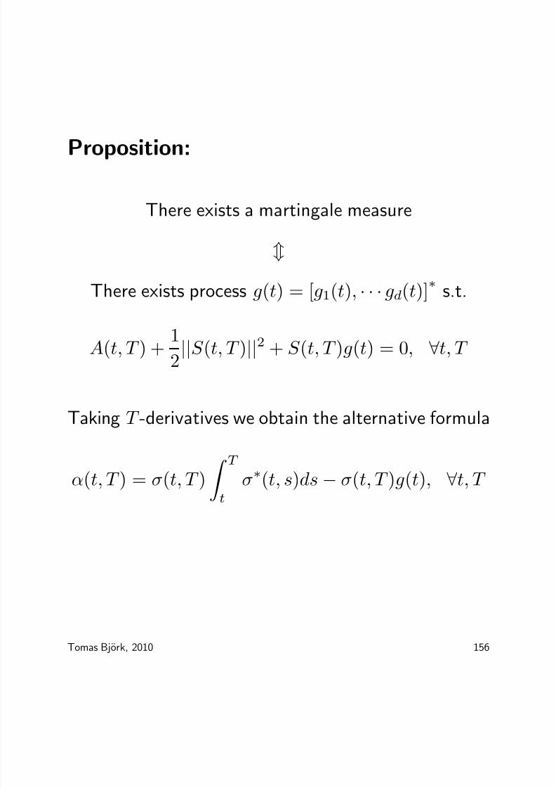
Proposition:
There exists a martingale measure
There exists process g(t) = [g1(t), · · · gd(t)]
∗s.t.
A(t, T ) + 1
2||S (t, T )||2 + S (t, T )g(t) = 0, ∀t, T
Taking T -derivatives we obtain the alternative formula
α(t, T ) = σ(t, T )
T t
σ∗(t, s)ds − σ(t, T )g(t), ∀t, T
Tomas Bjork, 2010 156

8/13/2019 Bjork Notes
http://slidepdf.com/reader/full/bjork-notes 158/202
Moral for Modeling
• Specify arbitrary volatilities σ(t, T ).
• Fix d “benchmark” maturities T 1, · · · , T d. For thesematurities, specify drift terms α(t, T 1), · · · α(t, T 1).
• The Girsanov kernel is uniquely determined (for eachfixed t) by
di=1
σi(t, T j)gi(t) =d
i=1
σi(t, T j)
T 0
σi(t, s)ds
− α(t, T j), j = 1, · · · d.
• Thus Q is uniquely determined.
• All other drift terms will be uniquely defined by
α(t, T ) = σ(t, T )
T
t
σ(t, s)ds−σ(t, T )g(t), ∀t, T
Tomas Bjork, 2010 157
8/13/2019 Bjork Notes
http://slidepdf.com/reader/full/bjork-notes 159/202
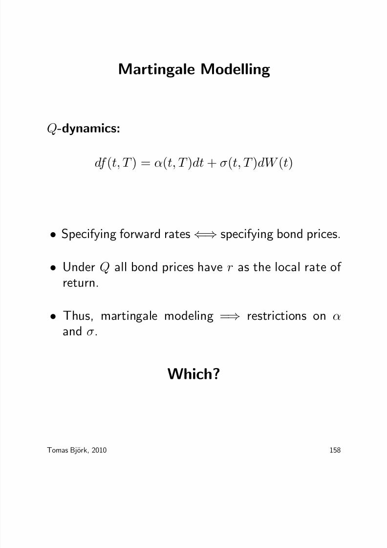
Martingale Modelling
Q-dynamics:
df (t, T ) = α(t, T )dt + σ(t, T )dW (t)
• Specifying forward rates ⇐⇒ specifying bond prices.
• Under Q all bond prices have r as the local rate of
return.
• Thus, martingale modeling =⇒ restrictions on αand σ.
Which?
Tomas Bjork, 2010 158

8/13/2019 Bjork Notes
http://slidepdf.com/reader/full/bjork-notes 160/202
Martingale modeling
Recall:
α(t, T ) = σ(t, T )
T
t
σ(t, s)ds − σ(t, T )g(t), ∀t, T
Martingale modeling ⇐⇒ g = 0
Theorem: (HJM drift Condition) The bond market isarbitrage free if and only if
α(t, T ) = σ(t, T )
T t
σ(t, s)ds.
Moral: Volatility can be specified freely. The forwardrate drift term is then uniquely determined.
Tomas Bjork, 2010 159

8/13/2019 Bjork Notes
http://slidepdf.com/reader/full/bjork-notes 161/202
Musiela parametrization
Parameterize forward rates by the time to maturity x,rather than time of maturity T .
Def:
r(t, x) = f (t, t + x).
Q-dynamics:
dr(t, x) = µ(t, x)dt + σ(t, x)dW.
What are the relations between µ and σ under Q?
Compare with HJM!
df (t, T ) = α(t, T )dt + σ0(t, T )dW.
where we use σ0 to denote the HJM volatility.
Tomas Bjork, 2010 160

8/13/2019 Bjork Notes
http://slidepdf.com/reader/full/bjork-notes 162/202
dr(t, x) = d [f (t, t + x)]
= df (t, t + x) + f T (t, t + x)dt
=
α(t, t + x) + rx(t, x)
dt + σ0(t, t + x)dW
µ(t, x) = α(t, t + x) + rx(t, x)
σ(t, x) = σ0(t, t + x).
HJM-condition:
α(t, T ) = σ0(t, T )
T t
σ0(t, s)ds.
Substitute!
Tomas Bjork, 2010 161

8/13/2019 Bjork Notes
http://slidepdf.com/reader/full/bjork-notes 163/202
The Musiela Equation
dr(t, x) =
∂
∂xr(t, x) + σ(t, x)
x0
σ(t, y)dy
dt
+ σ(t, x)dW
When σ is deterministic this is a linear equationin infinite dimensional space. Connections to control
theory.
Tomas Bjork, 2010 162

8/13/2019 Bjork Notes
http://slidepdf.com/reader/full/bjork-notes 164/202
Forward Rate Models
Pro:
• Easy to model flexible volatility structure for forwardrates.
• Easy to include multiple factors.
Con:
• The short rate will typically not be a Markov process.
• Computational problems.
Tomas Bjork, 2010 163

8/13/2019 Bjork Notes
http://slidepdf.com/reader/full/bjork-notes 165/202
7.
Change of Numeraire
Ch. 26
Tomas Bjork, 2010 164

8/13/2019 Bjork Notes
http://slidepdf.com/reader/full/bjork-notes 166/202
Change of Numeraire
Valuation formula:
Πt [X ] = E Q
e−R T t rsds × X
F t
Hard to compute. Double integral.
Note: If X and r are independent then
Πt [X ] = E Q
e−R T t rsds
F t · E Q [X | F t]= p(t, T ) · E Q [X | F t] .
Nice! We do not have to compute p(t, T ). It can beobserved directly on the market!Single integral!
Sad Fact: X and r are (almost) never independent!
Tomas Bjork, 2010 165

8/13/2019 Bjork Notes
http://slidepdf.com/reader/full/bjork-notes 167/202
Idea
Use T -bond (for a fixed T ) as numeraire. Define theT-forward measure QT by the requirement that
Π (t)
p(t, T )
is a QT -martingale for every price process Π (t).
Then
Πt [X ] p(t, T )
= E T
ΠT [X ] p(T, T )
F t
ΠT [X ] = X, p(T, T ) = 1.
Πt [X ] = p(t, T )E T [X | F t]
Do such measures exist?.
Tomas Bjork, 2010 166

8/13/2019 Bjork Notes
http://slidepdf.com/reader/full/bjork-notes 168/202
“The forward measure takes care of the stochasticsover the interval [t, T ].”
Enormous computational advantages.
Useful for interest rate derivatives, currency derivatives
and derivatives defined by several underlying assets.
Tomas Bjork, 2010 167

8/13/2019 Bjork Notes
http://slidepdf.com/reader/full/bjork-notes 169/202
General change of numeraire.
Idea: Use a fixed asset price process S t as numeraire.Define the measure QS by the requirement that
Π (t)
S t
is a QS -martingale for every arbitrage free price processΠ (t).
Tomas Bjork, 2010 168

8/13/2019 Bjork Notes
http://slidepdf.com/reader/full/bjork-notes 170/202
Constructing QS
Fix a T -claim X . From general theory:
Π0 [X ] = E Q
X
BT
Assume that QS exists and denote
Lt = dQS
dQ , on F t
Then
Π0 [X ]
S 0= E S ΠT [X ]
S T = E S X
S T
= E Q
LT
X
S T
Thus we have
Π0 [X ] = E Q
LT X · S 0
S T
,
Tomas Bjork, 2010 169

8/13/2019 Bjork Notes
http://slidepdf.com/reader/full/bjork-notes 171/202
For all X ∈ F T we thus have
E Q
X
BT
= E Q
LT
X · S 0S T
Natural candidate:
Lt = dQS
t
dQt
= S tS 0Bt
Proposition:
Π (t) /Bt is a Q-martingale.⇓
Π (t) /S t is a Q
-martingale.
Tomas Bjork, 2010 170

8/13/2019 Bjork Notes
http://slidepdf.com/reader/full/bjork-notes 172/202
Proof.
E S
Π (t)
S t
F s
=E Q
Lt
Π(t)S t
F s
Ls
=E Q
Π(t)BtS 0
F s
Ls
= Π (s)
B(s)S 0Ls
= Π (s)
S (s).
Tomas Bjork, 2010 171

8/13/2019 Bjork Notes
http://slidepdf.com/reader/full/bjork-notes 173/202
Result
Πt [X ] = S tE S
X
S t
F t
We can observe S t directly on the market.
Example: X = S t · Y
Πt [X ] = S tE S [Y | F t]
Tomas Bjork, 2010 172

8/13/2019 Bjork Notes
http://slidepdf.com/reader/full/bjork-notes 174/202
Several underlying
X = Φ [S 0(T ), S 1(T )]
Assume Φ is linearly homogeous. Transform to Q0.
Πt [X ] = S 0(t)E 0
Φ [S 0(T ), S 1(T )]
S 0(T )
F t
= S 0(t)E 0
[ϕ (Z T )| F t]
ϕ (z) = Φ [1, z] , Z t = S 1(t)
S 0(t)
Tomas Bjork, 2010 173

8/13/2019 Bjork Notes
http://slidepdf.com/reader/full/bjork-notes 175/202
Exchange option
X = max [S 1(T ) − S 0(T ), 0]
Πt [X ] = S 0(t)E 0
[max[Z (T ) − 1, 0]| F t]European Call on Z with strike price K . Zero interestrate.
Piece of cake!
Tomas Bjork, 2010 174

8/13/2019 Bjork Notes
http://slidepdf.com/reader/full/bjork-notes 176/202
Identifying the Girsanov Transformation
Assume Q-dynamics of S known as
dS t = rtS tdt + S tvtdW t
Lt = S tS 0Bt
From this we immediately have
dLt = LtvtdW t.
and we can summarize.
Theorem:The Girsanov kernel is given by thenumeraire volatility vt, i.e.
dLt = LtvtdW t.
Tomas Bjork, 2010 175

8/13/2019 Bjork Notes
http://slidepdf.com/reader/full/bjork-notes 177/202

8/13/2019 Bjork Notes
http://slidepdf.com/reader/full/bjork-notes 178/202
A new look on option pricing
European call on asset S with strike price K and maturity T .
X = max [S T − K, 0]
Write X as
X = (S T − K ) · I S T ≥ K = S T I S T ≥ K − KI S T ≥ K
Use QS on the first term and QT on the second.
Π0 [X ] = S 0 · QS [S T ≥ K ] − K · p(0, T ) · QT [S T ≥ K ]
Tomas Bjork, 2010 177

8/13/2019 Bjork Notes
http://slidepdf.com/reader/full/bjork-notes 179/202
Analytical Results
Assumption: Assume that Z S,T , defined by
Z S,T (t) = S t
p(t, T ),
has dynamics
dZ S,T (t) = Z S,T (t)mS T (t)dt + Z S,T (t)σS,T (t)dW,
where σS,T (t) is deterministic.
We have to compute
QT [S T
≥K ]
andQS [S T ≥ K ]
Tomas Bjork, 2010 178

8/13/2019 Bjork Notes
http://slidepdf.com/reader/full/bjork-notes 180/202
QT (S T ≥ K ) = QT
S T
p(T, T ) ≥ K
= QT (Z S,T (T )
≥K )
By definition Z S,T is a QT -martingale, so QT -dynamicsare given by
dZ S,T (t) = Z S,T (t)σS,T (t)dW T ,
with the solution
Z S,T (T ) =
S 0
p(0, T )×exp−
1
2 T
0 σ
2
S,T (t)dt + T
0 σS,T (t)dW
T Lognormal distribution!
Tomas Bjork, 2010 179

8/13/2019 Bjork Notes
http://slidepdf.com/reader/full/bjork-notes 181/202
The integral
T 0
σS,T (t)dW T
is Gaussian, with zero mean and variance
Σ2S,T (T ) =
T 0
σS,T (t)2dt
Thus
QT (S t ≥ K ) = N [d2],
d2 =
ln S 0
Kp(0,T )− 12Σ2
S,T (T ) Σ2S,T (T )
Tomas Bjork, 2010 180

8/13/2019 Bjork Notes
http://slidepdf.com/reader/full/bjork-notes 182/202
QS (S t ≥ K ) = QS
p(T, T )
S t≤ 1
K
= QS
Y S,T (T ) ≤ 1
K
,
Y S,T (t) = p(t, T )
S t=
1
Z S,T (t).
Y S,T is a QS -martingale, so QS -dynamics are
dY S,T (t) = Y S,T (t)δ S,T (t)dW S .
Y S,T = Z −1S,T
⇓δ S,T (t) = −σS,T (t)
Tomas Bjork, 2010 181
8/13/2019 Bjork Notes
http://slidepdf.com/reader/full/bjork-notes 183/202
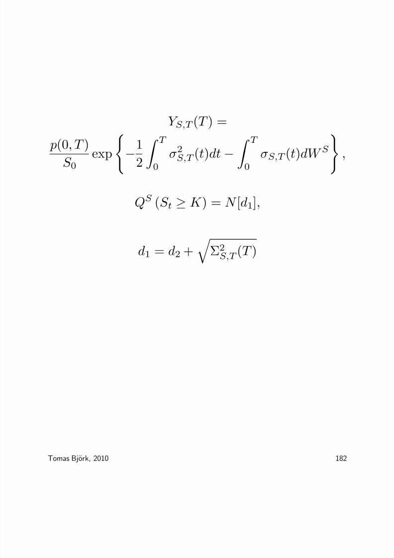
Y S,T (T ) =
p(0, T )
S 0exp
−1
2
T 0
σ2S,T (t)dt −
T 0
σS,T (t)dW S
,
QS (S t ≥ K ) = N [d1],
d1 = d2 +
Σ2S,T (T )
Tomas Bjork, 2010 182

8/13/2019 Bjork Notes
http://slidepdf.com/reader/full/bjork-notes 184/202
Proposition: Price of call is given by
Π0 [X ] = S 0N [d2] − K · p(0, T )N [d1]
d2 =ln
S 0Kp(0,T )
− 1
2Σ2S,T (T )
Σ2S,T (T )
d1 = d2 +
Σ2S,T (T )
Σ2S,T (T ) =
T
0 σS,T (t)
2dt
Tomas Bjork, 2010 183

8/13/2019 Bjork Notes
http://slidepdf.com/reader/full/bjork-notes 185/202
Hull-White
Q-dynamics:
dr = Φ(t) − ar dt + σdW.
Affine term structure:
p(t, T ) = eA(t,T )−B(t,T )rt,
B(t, T ) = 1
a
1 − e−a(T −t)
.
Check if Z has deterministic volatility
Z t = S t
p(t, T 1), S t = p(t, T 2)
Z t = p(t, T 2)
p(t, T 1)
,
Z t = exp ∆A(t) − ∆Btrt ,
Tomas Bjork, 2010 184

8/13/2019 Bjork Notes
http://slidepdf.com/reader/full/bjork-notes 186/202
Z (t) = exp ∆A(t) − ∆Btrt ,
∆A(t) = A(t, T 2) − A(t, T 1),
∆Bt = B(t, T 2)
−B(t, T 1),
dZ (t) = Z (t) ··· dt + Z (t) · σz(t)dW,
σz(t) = −σ∆Bt = σ
aeat
e−aT 1 − e−aT 2
Deterministic volatility!
Tomas Bjork, 2010 185

8/13/2019 Bjork Notes
http://slidepdf.com/reader/full/bjork-notes 187/202
8
LIBOR Market Models
Ch. 27
Tomas Bjork, 2010 186
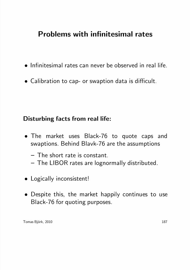
8/13/2019 Bjork Notes
http://slidepdf.com/reader/full/bjork-notes 188/202
Problems with infinitesimal rates
• Infinitesimal rates can never be observed in real life.
• Calibration to cap- or swaption data is difficult.
Disturbing facts from real life:
• The market uses Black-76 to quote caps and
swaptions. Behind Blavk-76 are the assumptions
– The short rate is constant.– The LIBOR rates are lognormally distributed.
• Logically inconsistent!
• Despite this, the market happily continues to useBlack-76 for quoting purposes.
Tomas Bjork, 2010 187

8/13/2019 Bjork Notes
http://slidepdf.com/reader/full/bjork-notes 189/202
Project
• Construct a logically consistent model which (tosome extent) justifies market practice.
• Construct an arbitrage free model with theproperty that caps, floors and/or swaptions arepriced with a Black-76 type formula.
Main models
• LIBOR market models (Miltersen-Sandmann-Sondermann, Brace-Gatarek-Musiela)
• Swap market models (Jamshidian).
Tomas Bjork, 2010 188

8/13/2019 Bjork Notes
http://slidepdf.com/reader/full/bjork-notes 190/202
• Instead of modeling instantaneous rates, we modeldiscrete market rates, such as
– LIBOR rates (LIBOR market models)
– Forward swap rates (swap market models).
• Under a suitable numeraire the market rates can bemodeled lognormally.
• The market models with thus produce pricingformulas of the type Black-76.
• By construction the market models are very easy tocalibrate to market data, i.e. to:
– Caps and floors (LIBOR market model)
– Swaptions (swap market model)
• Exotic derivatives has to be priced numerically.
Tomas Bjork, 2010 189

8/13/2019 Bjork Notes
http://slidepdf.com/reader/full/bjork-notes 191/202
Caps
Resettlement dates:
T 0 < T 1 < . . . < T n,
Tenor:
α = T i+1 − T i, i = 0, . . . , n − 1.
Typically α = 1/4, i.e. quarterly resettlement.
LIBOR forward rate for [T i−1, T i]:
Li(t) = 1
α· pi−1(t) − pi(t)
pi(t) , i = 1, . . . , N .
where we use the notation
pi(t) = p(t, T i)
Tomas Bjork, 2010 190

8/13/2019 Bjork Notes
http://slidepdf.com/reader/full/bjork-notes 192/202
Definition:A cap with cap rate R and resettlement datesT 0, . . . , T n is a contract which at each T i give theholder the amount
X i = α · max[Li(T i−1) − R, 0] , i = 1, . . . , N
The cap is thus a portfolio of caplets X 1, . . . , X n.
Tomas Bjork, 2010 191

8/13/2019 Bjork Notes
http://slidepdf.com/reader/full/bjork-notes 193/202
Black-76
The Black-76 formula for the caplet
X i = αi · max[L(T i−1, T i) − R, 0] , (1)
is given by
CaplBi (t) = α · pi(t) Li(t)N [d1] − RN [d2]
where
d1 = 1σi
√ T i − t
ln
Li(t)R
+ 1
2σ2i (T − t)
,
d2 = d1 − σi
T i − t.
• Black-76 presupposes that each LIBOR rate is
lognormal.• The constants σ1, . . . , σN are known as the Blackvolatilities
Tomas Bjork, 2010 192

8/13/2019 Bjork Notes
http://slidepdf.com/reader/full/bjork-notes 194/202
Market price quotes
Market prices are quoted in terms of Implied Blackvolatilities: The can be quoted in two different ways.
• Flat volatilities
• Spot volatilities (also known as forwardvolatilities)
Tomas Bjork, 2010 193

8/13/2019 Bjork Notes
http://slidepdf.com/reader/full/bjork-notes 195/202
Market Price Data
For each i = 1, . . . , N :
Capmi (t) = market price of cap with resettlement
dates T 0
, T 1
, . . . , T i
Implied market prices of caplets:
Caplmi (t) = Capmi (t) −Capmi−1(t),
with the convention Capm0 (t) = 0
Tomas Bjork, 2010 194

8/13/2019 Bjork Notes
http://slidepdf.com/reader/full/bjork-notes 196/202
Defining Implied Black Volatility
Given market price data as above, the implied Blackvolatilities are defined as follows.
• The implied flat volatilities σ1, . . . , σN are defined
as the solutions of the equations
Capmi (t) =i
k=1
CaplBk (t; σi), i = 1, . . . , N . (2)
• The implied forward or spot volatilities σ1, . . . , σN
are defined as solutions of the equations
Caplmi (t) = CaplBi (t; σi), i = 1, . . . , N . (3)
The sequence σ1, . . . , σN is called the volatility termstructure.
Tomas Bjork, 2010 195

8/13/2019 Bjork Notes
http://slidepdf.com/reader/full/bjork-notes 197/202
Theoretical Price of a Caplet
By risk neutral valuation:
Capli(t) = αE Qt
e−
R T i0 r(s)ds · max[Li(T i−1) − R, 0]
,
Better to use T i forward measure
Capli(t) = αpi(t)E T i [max[Li(T i−1) − R, 0]| F t] ,
The crucial point is the distribution of Li under Qi
where Qi = QT i
Important Fact: Li is a martingale under Qi
Li(t) = 1
α· pi−1(t) − pi(t)
pi(t)
Idea: Model Li as GBM under Q
i
:dLi = σiLidW i
Tomas Bjork, 2010 196

8/13/2019 Bjork Notes
http://slidepdf.com/reader/full/bjork-notes 198/202
LIBOR Market Model Definition
Define, for each i, the dynamics of Li under Qi as
dLi(t) = Li(t)σi(t)dW i(t), i = 1, . . . , N ,
where σ1(t), . . . , σN (t) are deterministic and W i isQi-Wiener.
The initial term structure L1(0), . . . , LN (0) is observedon the market.
Tomas Bjork, 2010 197
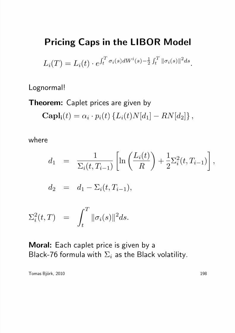
8/13/2019 Bjork Notes
http://slidepdf.com/reader/full/bjork-notes 199/202
Pricing Caps in the LIBOR Model
Li(T ) = Li(t) · eR T t σi(s)dW i(s)−1
2
R T t σi(s)2ds.
Lognormal!
Theorem: Caplet prices are given by
Capli(t) = αi · pi(t) Li(t)N [d1] − RN [d2] ,
where
d1 = 1
Σi(t, T i−1) ln
Li(t)
R +
1
2Σ2i (t, T i−1)
,
d2 = d1 − Σi(t, T i−1),
Σ2i (t, T ) =
T t
σi(s)2ds.
Moral: Each caplet price is given by aBlack-76 formula with Σi as the Black volatility.
Tomas Bjork, 2010 198

8/13/2019 Bjork Notes
http://slidepdf.com/reader/full/bjork-notes 200/202
Practical Handling of the LIBOR Model
We are standing at time t = 0.
• Collect implied caplet volatilities
σ1, . . . , σN
from the market.
• Choose model volatilities
σ1(
·), . . . , σN (
·)
such that
σi = 1
T i
T i−1
0
σ2i (s)ds, i = 1, . . . , N .
• Now the model is calibrated.
• Use numerical methods to compute prices of exotics.
Tomas Bjork, 2010 199

8/13/2019 Bjork Notes
http://slidepdf.com/reader/full/bjork-notes 201/202
Terminal Measure dynamics
Define the Likelihood process ηji as
ηji (t) = dQj
dQi, on F t
Can show that
dηi−1i (t) = ηi−1
i (t) αiLi(t)
1 + αiLi(t)σi(t)dW i(t).
Girsanov gives us
dW i(t) = αiLi(t)
1 + αiLi(t)σ
i
(t)dt + dW i−1(t).
Proposition The QN dynamics of the LIBOR rates are
dLi(t) =
−Li(t)
N
k=i+1
αkLk(t)
1 + αkLk(t)
σk(t)σi (t) dt
+ Li(t)σi(t)dW N (t),
Tomas Bjork, 2010 200

8/13/2019 Bjork Notes
http://slidepdf.com/reader/full/bjork-notes 202/202
Computational aspects
• The terminal measure dynamics of the system of LIBOR rates are quite messy.


![Analisis de Bjork - Jarabak [2]](https://img.dokumen.tips/doc/110x75/55cf97aa550346d03392e548/analisis-de-bjork-jarabak-2.jpg)