Bivariate traffic relations: A space-time modeling approachbivariate traffic relations 2.1 The general first-order model Past and present observations of traffic variables in the whole

Kamarianakis and Prastacos 1

Bivariate traffic relations: A space-time modeling approach

Yiannis Kamarianakis∗, Poulicos Prastacos

Regional Analysis Division, Institute of Applied and Computational Mathematics, Foundation for Research and

Technology, Vasilika Vouton, GR 71110, Heraklion Crete, Greece

Abstract Research on speed-flow-density relationships usually focuses on homogeneous road segments. This article aims at exploring these relationships at the macro setting of a road network based on time series observations collected from various measurement sites (spatial time series). For that purpose, we use tools from spatial statistics/econometrics, namely dynamic equilibrium correction models in space and time. Such models not only reproduce a static equation under stationary conditions but also depict short-term dynamics (i.e. equilibrium’s speed of adjustment). Moreover, the road network’s topology is incorporated in the modeling stage through specification of a weighting matrix. The adopted methodology is illustrated through the investigation of the flow-occupancy relationship in space and time. In our application, we use an extensive data set that corresponds to one months’ data, collected from major arterials of the road network of Athens, Greece.

Keywords: Bivariate traffic relations, space-time modeling, equilibrium correction 1. Introduction It is well accepted that distinct roadways accommodate different levels and patterns of vehicular flow, by virtue of their design. Traffic flow is described in terms of three parameters: the mean speed υ, the traffic flow rate q, and the traffic density k. The functional relationship between these three parameters is called Fundamental Diagram. The equilibrium relationship that associates them is q= υ k. Accordingly, the fundamental diagram is defined clearly if a function between two of the three parameters is defined. Since the bivariate functional relations between q, υ and k are directly related to the important problem of estimation of road capacity, research on these issues dates back to Schaar (1925). Two general approaches for stating speed-flow-density relationships may be distinguished. The classical approach has been a purely mathematical one. Firstly, an analytical expression containing several parameters is proposed and then the values of these parameters are estimated by fitting the expressions to traffic data. Finally, an interpretation of the parameters in terms of properties of traffic flow is sought, in order to provide the analytical expression with a phenomenological meaning. The famous speed–density models of Greenshields

∗ Corresponding Author. Tel.: +30 2810 391771; fax: +30 2810 391761. E-mail addresses: [email protected], [email protected].

mailto:[email protected]


(1935), Greenberg (1959), Underwood (1961) and Drake (1967) have been derived in such a manner. The second approach that may be called phenomenological or behavioral is based on assumptions about the driver behavior with respect to some traffic variables. The early procedures for estimating the capacity and those derived from car-following models belong to this approach. For some recent studies of that kind, the reader is referred to Kockelman (1998, 2001). Del Castillo and Benitez (1995a, 1995b) presented a methodology that combines both general approaches in a study of the speed density relationship. In contrast to the previously mentioned approaches that investigate the q-υ-k bivariate functional forms in homogeneous road segments, the methods presented in this paper can be applied in a larger scale that allows inference even for a whole road network. Based on the existing amount of traffic flow data which nowadays is large and of good quality, the models developed here are purely statistical and do not incorporate theoretical rationales such as hydrodynamic, car-following, etc. That is, instead of building a theoretical framework and then test it empirically with real world data (a significant amount of such research has been proven to encounter severe limitations), we let data to speak-up first and play a more decisive role in the modeling process. Traffic measurements are usually collected from loop detectors that provide traffic counts at constant time intervals. Consequently, these datasets are in the form of spatial time series. For data of that kind, one is interested in estimating multivariable relationships in space and time; that is detecting possible equilibria between traffic variables and estimating their adjustment speed after a shock (short run dynamics). Under the assumption that a sufficiently large number of measurement sites exist at the network under study so that the researcher is allowed to ignore potential inferential biases due to their position, conjectures of that kind can be achieved via Dynamic Space Time models and their equilibrium correction formulation. Thus, this research presents a modeling strategy that allows for the examination of

- Long-term traffic flow dynamics for the whole network: The equilibrium relationships between υ- q, υ- k and/or q-k in the road network.

- Short-term dynamics of the network: Equilibrium’s speed of adjustment after a shock. - Long-term dynamics for each measurement location: Location specific equilibria. - Short-term dynamics for each measurement location: How fast the location-specific

equilibrium is approached after a shock in this location or how fast the location-specific equilibrium is approached after a shock in a neighboring location.

The aforementioned model class and the subsumed models that fit better on the needs of our problem, together with technical details on estimation and model selection are presented next. The third section contains a detailed numerical illustration; the proposed methods are performed on a month’s data taken from eleven loops located at major arterials of the city of Athens. The last section is devoted to some concluding remarks.


2. Dynamic space-time models and their equilibrium correction formulation for bivariate traffic relations

2.1 The general first-order model

Past and present observations of traffic variables in the whole network can be related via a dynamic model in space and time. One may encounter such models in the econometrics literature as “serial and spatial autoregressive distributed lag models”. The interested reader can find an introduction to distributed lag models at Greene (1997). Elhorst (2001) presents a detailed treatment of first order Dynamic Space-Time models and their equilibrium correction formulation. For the moment, we also consider first order models, which relate present observations to the instant past. Considered in vector form for a cross-section of observations at time t the general model is of the form shown below 1: ttttttttt WxWxxxWyWyyy εδδγγββαµ ++++++++= −−−− 1101101101 . (1) A variable with subscript t-1 denotes its serially lagged value, and a variable pre-multiplied by W denotes its spatially lagged value. denotes a ty 1×n

10 ,

vector consisting of one observation of the dependent variable for every measurement location (i=1,..,n) at time t; denotes a vector of the explanatory variable (for reasons of simplicity, only one regressor is considered at the moment).

tx1×n

101 ,,,,, 0, δδγγββαµ are the response parameters and tε is a normally distributed vector containing the error terms with 1×n ( ) 0=tE ε and

. ( )ttε ′ nI2σE ε = { }0≥, ijw,...,1,: =∀= ij njiwW denotes an nn× matrix describing causality relations related to the spatial arrangement of the measurement locations. Thus, reflects that a change in traffic conditions close to i is expected to affect traffic conditions close to j. Since no measurement location can be viewed as a neighbor of itself, weight matrices have zero diagonal elements. We put more emphasis on the different forms that a spatial weight matrix can take, in the next subsection.

0>ijw

The general model depicted in (1) relates current observations of let’s say average speed at site i to the immediately previous ones taken from that location, to current and previous linear combinations (that are explicitly defined through the rows of the weight matrix) of measurements that correspond to neighboring sites, to past and current observations of let’s say average density at site i, and to past and current combinations of densities that correspond to neighboring sites. The plausibility of the proposed model is straightforward but it should be underlined that we are not expected to be able to estimate the general form accurately because of multicollinearities2; one should estimate suitable sub-models in order to make inference. For example, it should be expected that the two terms corresponding to spatially weighted densities are highly correlated with current and past observations of densities; if this is confirmed, we should better drop one of the two pairs of variables out of the model.

1 In contrast with Elhorst (2001) there is an intercept term in (1). Its importance wiil be evident in the application. 2 Multicollinearity appears when the explanatory variables in a regression model are too highly intercorrelated to allow precise analysis of their individual effects. The interested reader may consult Greene (1997) chapter 9 for this issue.


2.2 The spatial weight matrix Weight matrices as the one in equation (1) have been implicitly assumed in short term traffic forecasting models. In studies of that kind, measurements taken from upstream measurement locations (only) are supposed to have explanatory power for the ones taken from downstream sites thus resulting to the implicit adoption of a lower diagonal weight matrix (see for example Stathopoulos and Karlaftis, 2003). Kamarianakis and Prastacos (2002, 2003) have explicitly assumed such a matrix while using Space-Time ARIMA methods for short-term forecasting in urban networks. To clarify things, we present part of a hypothetical network and the weight matrix that corresponds to equal weights to nearest neighbors3. In figure 1 one may recognize the tree structure of a road network with dots representing measurement locations and arrows the direction of flow.

=

0100000000000005.05.0000000000000000000000000005.05.0000000000000000000000000005.05.000000000000005.05.0000000000000033.033.033.000000000000000000000000000000000000000000000000000000000000000000

13121110987654321

13121110987654321

1W

Figure 1. Measurement locations at a road network and the spatial weight matrix that corresponds to equal

weights for nearest upstream neighbors. It is important to keep in mind that all subsequent analyses are conditional upon the choice of the spatial weight matrix and that there are plenty of choices for its form. For example, a researcher may drop the assumption that only upstream locations are causal to downstream ones and take the k-nearest neighbors or the neighbors that lie at a predefined distance regardless of being upstream or downstream. Another option that seems rational when urban networks are under investigation is the adoption of two weight matrices; one corresponding to upstream causalities and one for downstream ones. Such matrices can be part of a threshold autoregressive model where traffic conditions are divided into homogeneous regimes. Hence, one will be able to estimate the relative explanatory power of upstream/downstream locations to the traffic conditions of a reference location. As noted in the previous subsection, one strategy is to assign equal weights to all neighbors of a measurement location, considering that the useful information on the evolution of our response given from its neighbors is of equal quantity across them; a second approach is to assign weights proportional to inverse distance, treating favorably the closer neighbors. For forecasting applications, weights can be proportional to the crosscorrelations of measurements that correspond to different locations. Nonzero elements of each row will correspond to coefficients of a vector autoregressive model where the vector contains measurements from the reference site and all its “neighbors”. We should finally note that in the vast majority of spatial modeling applications, rows of the spatial weight matrix are standardized to sum to one. 3 Alternatively weights could be proportional to inverse distance from the reference location.


2.3 The equilibrium correction formulation Let’s start from the first order serial autoregressive distributed lag model (a sub-model of (1) with no spatial dependencies) ttttt xxayy εγγµ ++++= −− 1101 (2) which can be equivalently reformulated as

ttttttttt uxcxbyaxxyy +∆++∆+=−

+∆−

−−+

+∆−

−−

= ˆˆˆˆ1

11111

110 µεαα

γαγγ

αα

αµ . (3)

Now short-run dynamics have been added to the static equation. That is equation (3) not only contains the static long run equilibrium relationship between y and x in the whole network but also captures short-run dynamics of how equilibrium is approached. b reflects the long-run effect of y with respect to x, while c reflects the short-run immediate response of y to a change in x.

ˆˆ

Long-run dynamics of each location’s equilibria while taking into account their spatial arrangement within the network are given after reformulating the equation ttttt WxxWyy εγβαµ ++++= (4) to ( ) ( ) ( )[ ] ttNNNt uxWWIWIWIy +−+−+−= −−− 111 αγαβµα . (5) Via this formulation, observations from a measurement site are not only influenced by its local conditions, but also by those of its neighbors depending on the structure of the spatial weight matrix. Furthermore, the impact of these conditions is not necessarily uniform across spatial units. In order to assess both (spatially dependent) long and short-term dynamics for each location one has to manipulate the general first order equation (1) to take the form ( ) ( ) ( ) ( ) ttttttt xWxWxxyWyWWLI εδγδδγγβαµββα +∆−∆−++++∆+−=−−− 111010110 .

(6) This equation entails a static equilibrium relation between y and x and describes how this equilibrium is approached after a change on the levels of the explanatory not only at the location of interest, but at neighboring influential locations as well. In order to illustrate equilibrium correction modeling we present a simple example. Following Greene (1997), we examine the relation between flow and occupancy at a single location. Empirical findings suggest that a linear model of squared occupancies on flows fits observed data quite well. Let stand for observed flows at time t and for squared occupancies. If the level of has been unchanged for many periods prior to t, the equilibrium value of

ty

txtx

[ ]tyE (assuming it exists) will be

∑∑∞

=

∞

=

+=+=10 i

ii

i xaxay ββ (7)


where x is the permanent value of . For this to be finite, we must have tx ∞<∑∞

=0iiβ .

Consider now the effect of a ten percent change in x occurring in period s. Prior to the shock in occupancies, flows had reached equilibrium. The path to the new equilibrium might appear as shown in figure 2. The short-run effect is the one which occurs in the same period as the change in x . This is 0β in the figure; this is the short-run multiplier. The differences between the old equilibrium D0 and the new one D1, is the sum of individual period effects.

That is the total effect is equal to ; β is the equilibrium multiplier. ∑∞

=0ι

= ββ i

Figure 2: Lagged adjustment of traffic flow equilibria.

2.4 Technical details The serial lagged dependent variable among regressors causes the OLS estimators to lose their unbiasedness property. The spatial-econometrics literature has shown that the inclusion of a spatial lag of the dependent on the right hand side of the equation not only makes the OLS estimator to lose its unbiasedness but it loses its consistency as well. The most commonly suggested method to overcome this problem is estimation via maximum likelihood (see Anselin, 1988, pp. 181-182). Elhorst (2001) provides the (conditional upon the vector of first observations) log-likelihood function of the general first order model given by equation (1):

( ) ( ) ( ) ∑=

′−−−+−−=−

T

tttYYYY WITTnLogf

TT2

22

,...,, 21log12log1

21

121εε

σαπσ (8)

Thus, if one wants to test against different model generating formulations through Wald, Lagrange multiplier or likelihood ratio tests4 and a spatial-lag model lies among the ones 4 For a detailed treatment on tests for model selection, see Greene (1997) chapter 11. The aforementioned tests apply for nested hypotheses. Elhorst (2001) encountered difficulties and did not provide clear results when non-nested models had do be compared in model selection procedures. It seems that a recent paper by Rivers and Vuong (2002) enlightens that area.


tested, he/she should estimate all of them via maximum likelihood. To facilitate maximum likelihood estimation of the α coefficient that reflects instantaneous spatial association in (1) and to ensure invertibility of the matrix ( )WI α− , Ord (1981) demonstrates the following requirement

maxmin

11ω

αω

<< (9)

where ωmin, and ωmax are the minimum and maximum characteristic roots of the spatial weight matrix W. Elhorst (2001) provides a general condition so that the general space-time process (1) is stationary in time: ( )( ) 11

01 <−+ −WIWI ββα . (10)

He also describes in detail stationarity conditions on restricted models. These restrictions are captured by the log-likelihood functions in that these functions are not defined for parameter values that do not satisfy these conditions.

3. The application

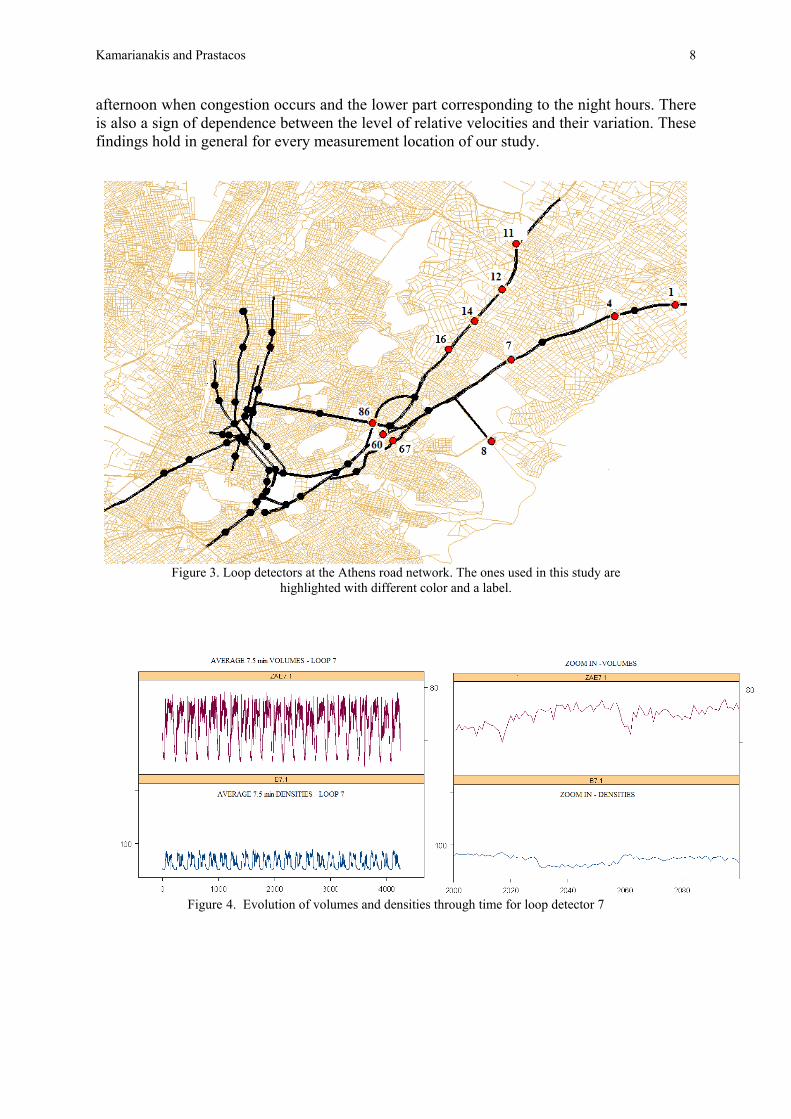
3.1 The study area and the data analyzed The urban area of Athens, the capital of Greece, has an area of 60 km2 and a population of approximately four million people. Total daily demand for travel is about 5.5 million trips with about 1 million occurring during the 2-hour peak period. A set of 88 loop detectors has been installed by the Ministry of Environment and Public Works at major roads of the Athens network to measure traffic volume and road occupancy. Measurements take place every 90 seconds and are immediately transmitted to the Urban Traffic Control Center where they are used by the Siemens MIGRA traffic control system to adjust street lights timing and stored in databases for further analysis, see Kotzinos (2001). An indicator of data quality ranging from 1 to 3 is transmitted as well since often electronic or system failures result in measurements that might not be accurate. The dataset used for the illustration of the methodology consists of observations that correspond to eleven loop detectors (figure 2). For all loops, traffic direction is towards the center of the city5. A typical period –in terms of traffic flow- was selected to be studied: from February 11 2002, to March 10, 2002. Observations corresponding to weekends were discarded since traffic flow patterns differ significantly these days. The initial dataset contained a time series of 21210 observations for every loop detector. To ease implementation and smooth out noise, averages over five consecutive 90-second intervals were taken, thus resulting in a total of 4242 observations per detector, 192 measurements per day for each loop. Observations from loop detector seven are depicted at figure 4. A sinusoidal pattern can be observed in both volumes and occupancies, the higher part corresponding to morning until

5 The total number of loops located at streets with direction towards the center of Athens is thirty six. Twenty five of them provided data of high quality at the period of our study; the eleven loops we use are a subset of these twenty five.


afternoon when congestion occurs and the lower part corresponding to the night hours. There is also a sign of dependence between the level of relative velocities and their variation. These findings hold in general for every measurement location of our study.

Figure 3. Loop detectors at the Athens road network. The ones used in this study are

highlighted with different color and a label.

Figure 4. Evolution of volumes and densities through time for loop detector 7


3.2 Preliminary data investigation The first step of the analysis was to investigate the flow-occupancy relationship for each loop detector separately. Seeking for an optimal linear model that best describes the relation, we applied the nonparametric method proposed by Young et al. (1976)6. Essentially, this method seeks for optimal transformations that need to be applied to a pair of variables so that their relationship becomes linear; the criterion used is maximization of R2. For all loops, we observed that a polynomial of third order is better suited for occupancies. For volumes, results were not easily interpretable though; see for example figure 5, which displays the nonparametric smoothing spline transformations for loop seven. We continued via using the parametric method proposed by Box and Cox (1964). The Box-Cox method was applied to volumes given that they had to be expressed as third order polynomials of occupancies. In any case, no deviation from the original scale was indicated7. We thus performed linear regressions8 of third order polynomials of occupancies (explanatory part) to observed volumes, for each loop. Results are presented at table 1; figure 6 depicts some volume-occupancy scatterplots together with the polynomial regression curves. What one first observes from the R2 statistics is the very satisfactory fit of the third order polynomial curves to the observed flow-occupancy relationships (except for loop 67) and the closeness of the R2 of the regression when compared with the maximum R2 that can be achieved from a nonparametric transformation of volumes and occupancies (last column). One should also note the similarity of regression coefficients for loops located at the same road. Regression errors were found to be both heteroscedastic and autocorrelated; that is one expects different levels of error on the prediction of volumes, at different levels of occupancies. Moreover the observed errors differ significantly from the i.i.d. regression hypothesis, displaying short term dependencies of large size. Heteroscedasticity and autocorrelation properties are directly related to the fact that both volumes and occupancies display larger variation at their high levels (mean dependent variation) and are time dependent variables. For normally distributed errors, these properties make the ordinary least squares estimators to lose their efficiency property. Given the size of our sample this is not a significant problem; what is important in our case is that our estimations continue being unbiased.

FIGURE 5.Transformations that linearize the relationship between volumes and occupancies.

6 SAS/STAT PROC TRANSREG (Morals algorithm) used on that purpose. 7 The Box-Cox method uses maximum likelihood to find an optimal power transformation of the response variable. It not only provides transformations that linearize a relationship but it homogenizes variance as well. In our application we observed that variance levels of volumes were significantly different at different occupancy levels. 8 Regressions were performed after statistically significant outliers were identified and deleted (Table1 column 8).


INTERCEPT LINEAR QUADRATIC CUBIC REG R2

RMSE Outliers Num.

SM. SPLINE R2

Loop 1 5.517 (0.2)

5.1 (0.036)

-0.139 (0.0014)

0.0011 (148 E-7)

0.89 5.56 21 0.93

Loop 4 5.84 (0.19)

4.7 (0.03)

-0.12 (0.001)

0.009 (484 E-7)

0.91 5.11 7 0.96

Loop 7 6.22 (0.178)

4.38 (0.028)

-0.1 (0.001)

0.0006 (983 E-8)

0.93 4.62 0 0.947

Loop 8 -0.553 (0.226)

3.855 (0.037)

-0.062 (0.0013)

0.0003 (128 E-7)

0.96 4.82 4 0.96

Loop 11 4.54 (0.177)

6.485 (0.035)

-0.2 (0.0018)

0.0018 (242 E-7)

0.95 4.68 24 0.96

Loop 12 9.95 (0.2)

3.475 (0.03)

-0.08 (0.0011)

0.0005 (979 E-8)

0.83 5.74 0 0.933

Loop 14 7.735 (0.22)

4.2 (0.043)

-0.1 (0.0015)

0.0006 (136 E-7)

0.86 5.62 6 0.9

Loop 16 4.2 (0.19)

4.46 (0.03)

-0.1 (0.0012)

0.0006 (127 E-7)

0.95 4.12 12 0.95

Loop 60 2.12 (0.1)

1.7 (0.01)

-0.046 (0.0005)

0.0003 (404 E-8)

0.84 2.26 14 0.86

Loop 67 2.13 (0.26)

1.74 (0.03)

-0.04 (0.0008)

0.0003 (64 E-7)

0.55 6.087 0 0.59

Loop 82 2.741 (0.1)

0.85 (0.01)

-0.015 (0.0004)

0.0001 (363 E-8)

0.83 2 1 0.84

Table 1. Third order polynomial regression of volumes on occupancies.

Figure 6. Occupancy-Volume scatterplots and third-order regression curves for four loops of the study.


3.3 Model fitting The first step of the modeling stage was the construction of a weight matrix that reflects causality relations in the set of the eleven loops of the study. To simplify the analysis, we adopted the hypothesis of “upstream causality”; that is traffic conditions at upstream locations are causal to what we observe downstream and not vice-versa.9 For comparative purposes, we constructed two spatial weight matrices; the first contained only the nearest upstream neighbors for loops 4, 7, 12, 14 and 16. The second one contained all upstream neighbors with equal weights (figure 7). Each pair of spatial lags of volumes and occupancies – ( ) - contained almost perfectly correlated variables (Pearson correlation >0.97 for both cases) and because of that, modeling results were practically the same with either matrix. The modeling results presented next, correspond to the choice of the first weight matrix.

( tttt xWxWyWyW 2121 ,,, )

25.0005.000025.025.0008600000005.05.0006700033.000033.033.000600000100000016000001000001400000010000120000000000011000000000008000000000107000000000014000000000001

866760161412118741

1

loop

W =

25.0005.000025.025.0008600000005.05.0006700033.000033.033.00060000033.033.033.0000016000005.05.0000014000000100001200000000000110000000000080000000005.05.07000000000014000000000001866760161412118741

2

loop

W =

Figure 7. The two weight matrices used

At the previous subsection, when modeling took place for each detector separately, it was shown that volumes can be well represented by third order polynomials of occupancies. In the “pooled-loop” case where we examine models of the form ttt bxay ε++= (11) and are vectors of observations at time t corresponding to a set of loops, this is not the case. Due to high correlation (Pearson’s r >0.95) between pooled occupancies and pooled squared occupancies and much higher correlation of occupancies with volumes (Pearson’s r =0.45) than with squared occupancies (Pearson’s r =0.29) one should estimate models (1), (2), (4) with occupancies as the explanatory variable and not with squared occupancies or both.

tt xy ,

To assess long and short run dynamics for the whole network, one has to estimate equation (2). However, occupancies and serially lagged occupancies are so correlated (Pearson’s r >0.97) that the specified regression model (2) would be susceptible to multicollinearity symptoms; the most important of these is that small changes in the data can produce large swings in the parameter estimates. There is no problem however for direct estimation of the

9 “Downstream causality” is expected to hold when traffic is at the stage of congestion. One may estimate the explanatory power of upstream versus downstream locations for a reference site at different states of traffic, via adopting two weight matrices (one for upstream and one for downstream locations) and a regime switching methodology.


last part of equation (3) via maximum likelihood10. Estimation results and model fit statistics11 are displayed in table 2. It appears that a constant term is highly significant and contributes to the accuracy of the distributed lag model: . (12) ttttt xcxbyay εµ +∆++∆+= ˆˆˆˆ Suppose our estimates were obtained from a large dataset of loop detectors that represents unbiasedly the traffic conditions of the network under study and a researcher wants to have an idea on the long and short term volume-occupancy dynamics at a location far from any detector. Using the estimated coefficients one can estimate these dynamics supposing essentially that the unknown location is an “average” one in terms of traffic conditions.

µ α b c AIC SBC Stand. Error

Eq. (12)

22.72 (0.13)

0.494 (0.015)

0.45 (0.0039)

-0.229 (0.01)

400479.5 400514.6 17.68

Table 2. Maximum likelihood estimates and model fit for models (3) and (6) . We continue with the direct estimation of model (4) via maximum likelihood. This model illustrates the equilibrium dynamics of all studied locations while accounting for their dependencies with other parts of the network, as they are denoted by the spatial weight matrix. Suppose average occupancies are expected to change at a particular location close to a loop (let’s say due to constructions). This model provides estimates of the (average) volumes at locations affected by that change.

µ α β γ AIC SBC Stand. Error

Eq. (4)

27.45 (0.15)

-0.19 (0.005)

0.5 (0.004)

-0.015

399390 399425 17.47

Table 3. Maximum likelihood estimates and model fit for model (4).

4. Conclusions and directions for further research Based on current advances in space-time modeling, this work demonstrates a methodology that allows for extracting useful information from traffic variables collected from numerous locations of a road network. We have demonstrated how one may estimate both long and short-term dynamics in bivariate traffic relations and how one can assess effects of changes in traffic conditions at a reference location to neighboring ones. It should be underlined that the proposed models are conditional upon the choice of a spatial weight matrix that reflects spatial dependencies, that is causal relations between neighboring sites. Until now, in all spatial modeling applications these matrices were exogenously defined resulting in some arbitrariness in the modeling stage. In subsection 2.2 we explore the possible forms that an exogenously defined spatial weight matrix may take

10 Marquardt’s algorithm used on that purpose. 11 The Swartz Bayesian Criterion (SBC) and Akaike’s Information Criterion (AIC) are penalized likelihood statistics that indicate model fit. The less their value the better model fit is. The standard error estimate at the last column of table 2 corresponds to the square root of the residual variance.


according to a researcher’s inferential needs. We also mentioned a way that allows an endogenous definition for the spatial weights. To illustrate the proposed method we performed a detailed numerical application using volume-occupancy measurements collected from various locations of an urban network. We first analyzed each measurement site separately and that allowed us to observe a great degree of variation in the volume-occupancy relation due to each location’s specific characteristics. Next, we proceeded to the space-time modeling stage where the reader may notice some difficulties encountered and how they can be circumvented. Traffic variables are characterized by a periodic pattern. A next step in this research should be the adoption of a regime switching methodology that allows for different long and short-term dynamics when traffic conditions fall into different regimes. We should finally note that special forms of the proposed models –the ones with no contemporaneous spatio-temporal dependencies- can be used for short-term forecasting. A general first order model that can be used for that purpose comes from a modification of equation (1) tttttt WxxWyyy εδγβα ++++= −−−− 1111111 (13) and it is straightforward to define higher order models. The main advantage of this approach in short term traffic forecasting is that one uses a single model to forecast observations taken from various locations. There is a clear resemblance of equation (8) and the Space Time Arima models used by Kamarianakis and Prastacos (2002, 2003).

References

Anselin, L., 1988. Spatial Econometrics: Methods and models. Kluwer.

Box, G., Cox, D., 1964. An analysis of transformations. Journal of the Royal Statistical society, Series B, 389-398.

Del Castillo, J.M., Benitez, F.G., 1995a. On the functional form of the speed-density relationship – I: General theory. Transportation Research B, Vol 29B.

Del Castillo, J.M., Benitez, F.G., 1995b. On the functional form of the speed-density relationship – II: Empirical investigation. Transportation Research B, Vol 29B.

Drake, J.S., Schofer, J.L., May. A.D. , 1967. A statistical analysis of speed-density hypotheses. Highway Research Record, Vol. 156. Elhorst, J.P., 2001. Dynamic models in space and time. Geographical Analysis, Vol 33.

Greenberg, H., 1959. An analysis of traffic flow. Operations Research, Vol. 7. Greene, W.H., 1997. Econometric Analysis (third edition). Prentice Hall. Greenshields, B. D., 1935. A study in highway capacity. Highway Research Board Proceedings, Vol. 14. Kamarianakis, Y., 2003. Spatial time series modeling: A review of the proposed methodologies. REAL working paper, University of Illinois at Urbana Champaign, 2003. Kamarianakis, Y., Prastacos, P., 2002. Space-time modeling of traffic flow. Paper presented at the European Regional Science Association Conference. Availlable from www.ersa2002.org Kamarianakis, Y., Prastacos, P. ,2003. Forecasting traffic flow conditions in an urban network: Comparison of univariate and multivariate approaches. Journal of the Transportation Research Board. Kockelman, K.M., 1998. Changes in the flow-density relation due to environmental, vehicle, and driver characteristics. Transportation Research Record 1644. Kockelman, K.M., 2001. Modeling traffic’s flow-density relation: Accommodation of multiple flow regimes and traveler types. Transportation, Vol. 28, 2001. Kotzinos, D. , 2001. Advanced Traveler’s Information Systems. Ph.D. dissertation, Technical University of Crete, Chania, Greece, 2001. Ord, J.K., 1981. Towards a theory of spatial statistics: A comment. Geographical Analysis, Vol 13. Rivers, D., Vuong, Q., 2002. Model selection tests for nonlinear dynamic models. Econometrics Journal, Vol 5. Schaar, 1925. Die leistungsfahigkeit einer strabe fur den kraftverkehr. Verkehrstechnik Vol. 23. Stathopoulos, A., Karlaftis, M.G., 2003. A multivariate state space approach for urban traffic flow modeling


and prediction. Transportation Research Part C, 11, 121-135. Underwood, R.T., 1961. Speed, volume and density relationships. Quality and theory of traffic flow, Yale Bureau of Highway Traffic. Young, F.W., de Leeuw, J., Takane, Y., 1976. Regression with qualitative and quantitative variables: an alternating least squares approach with optimal scaling features, Psychometrika, 41, 505 -529.

Documents

Bivariate traffic relations: A space-time modeling approachbivariate traffic relations 2.1 The general first-order model Past and present observations of traffic variables in the whole