Bivariate Splines for Ozone Concentration Forecasting

Bree EttingerDepartment of MathematicsThe University of GeorgiaAthens, GA 30602, USA

Serge Guillas∗

Department of Statistical ScienceUniversity College London

UK

Ming-Jun Lai†

Department of MathematicsThe University of GeorgiaAthens, GA 30602, USA

∗Corresponding author, partly supported by the London Mathematical Society.†This author is partly supported by the National Science Foundation under grant DMS-0713807

1

Abstract

In this paper, we forecast ground level ozone concentrations over the USA, using past spa-tially distributed measurements and the functional linear regression model. We employ bivariatesplines defined over triangulations of the relevant region of the USA to implement this func-tional data approach in which random surfaces represent ozone concentrations. We compare theleast squares method with penalty to the principal components regression approach. Moderatesample sizes provide good quality forecasts in both cases with little computational effort. Wealso illustrate the variability of forecasts due to the choice of smoothing penalty. Finally, wecompare our predictions with the ones obtained using thin-plate splines. Predictions based onbivariate splines require less computational time than the ones based on thin-plate splines andare more accurate. We also quantify the variability in the predictions arising from the variabil-ity in the sample using the jackknife, and report that predictions based on bivariate splines aremore robust than the ones based on thin-plate splines.

Keywords: functional data, ozone, bivariate splines.

1 Introduction

Ground-level ozone is a harmful pollutant (Bell et al., 2004). To inform the public on a daily basisabout ozone and other pollutants, the US Environmental Protection Agency (EPA) has createda simplified index of air quality, the pollutant standards index (PSI), and since July 1999, EPAreplaced the PSI with the Air Quality Index (AQI). Forecasts of these indices made 24 hoursahead have been provided to newspapers in various regions so that people can avoid outdooractivities likely to damage their health. Using the PSI, Neidell (2010) showed that air qualitywarnings associated with ground-level ozone have had an impact on outdoor activities in SouthernCalifornia, especially for susceptible local residents. Hence, improving the quality of these forecastsmay contribute to better public health.We consider here ozone concentrations from the network of EPA stations across the USA, over aspan of three months in the summer of 2005. Our goal is to predict the ozone concentration values ata specific location in suburban Atlanta 24 hours ahead based on the previous ozone concentrationsvalues up to the current hour. There are many available methods, ranging from chemistry-transportmodels to statistical techniques. Recently, Guillas and Lai (2010) initiated a brand new statisticalapproach to predict ozone concentration values using functional linear regression with bivariatesplines (piecewise polynomial functions over a triangulation of a polygonal domain). The goal is tocapture predictive power in time from spatial synoptic scales, as chemistry and transport occur atregional scales. Such spatio-temporal information has been used before to model time-dependentdynamics in hourly ozone concentration fields, see e.g. Dou et al. (2010). However, our approachrepresents the surface as a random function, which enables us to carry out regression and predictionin that setting. Modelling observations as functional data presents many advantages, see Ramsayand Silverman (2005) and Ferraty and Vieu (2006) for an overview of functional data analysis(FDA). For that purpose, one needs a parametric representation of the surfaces ideally in a flexiblebasis that kriging is not able to offer. Guillas and Lai (2010) established the theoretical foundations,even under time-dependence assumptions, of this method for which a least squares criterion withpenalty is minimized. In the following, we refer to this approach as the “brute force method” (BF).Comparison with time series approaches using FDA (i.e. in one dimension: time) shows that BFcan predict better, particularly with small sample sizes by borrowing strength across space aroundthe location of interest, see Guillas and Lai (2010) for examples.Crambes et al. (2009) minimized a residual sum of squares subject to a smoothness penalty as inBF, but modified the usual penalty term of univariate smoothing splines to study the prediction.

2

They showed that the rates of convergence of the estimates of the slope are optimal. Yuan andCai (2010) demonstrated that BF can deliver optimal rates of convergence for either prediction orestimation. Their setting unifies the treatment of estimation and prediction under the umbrellaof one family of norms. They showed the interesting property that the faster the decay in theeigenvalues of the covariance operator of the explanatory variable, the faster the prediction and theslower the estimation of the slope.The Functional Principal Component Regression (FPCR) has been introduced in two papers (Car-dot et al., 1999, 2003), which cover the case of random functional data that are curves. It relies onthe principal component decompositions prior to inference about the regression slope. Cardot et al.(2003) used univariate splines to approximate the empirical estimator for the regressor function as-sociated with the random functional. FPCR was shown to attain optimal rates of convergencefor prediction and estimation (Cai and Hall, 2006; Hall and Horowitz, 2007). As pointed out byCressie and Wikle (2011), the Empirical Orthogonal Functions (EOFs) employed in space-timeanalysis of geophysical data are merely principal components for the vector of observations. Inpractice, EOFs are used since observations are collected at discrete points. However, this approachcan yield misleading results as these observations are not weighted spatially. The analysis shouldreflect the continous variations of the field. The Karhunen-Loeve expansion considered below is thecontinuous equivalent of the EOF decomposition. Using bivariate splines, we respect the continuousnature of ozone fields.In our context of ozone forecasting, Aneiros-Perez et al. (2004) considered a functional additivemodel and Crambes et al. (2009) applied least squares with penalty to the prediction of the maxi-mum of the ground-level ozone concentration. However, these studies do not exploit spatial infor-mation. When dealing with random surfaces and a functional associated with these over a domainof irregular shape, bivariate splines can be an excellent approximation tool, especially when therandom surfaces are observed only over scattered locations (Lai, 2008) as these splines possessoptimal approximation properties (Lai and Schumaker, 2007). Thus, we shall use these splinesin FPCR and would like to know how it compares with BF for the ozone concentration forecast-ing problem. We shall explain this generalization in the following section in detail and discussthe similarities and differences between BF and FPCR in this context. We illustrate numericallythe advantages and disadvantages of these two approaches. The biggest difference lies in the factthat BF is straightforward and can be used for prediction without a spectral decomposition whilethe FPCR requires the use of a selected number of eigenvalues and eigenvectors in advance to beeffective for prediction.Thin-plate splines have been used in various applications to model surfaces, see Wood (2003) andreferences therein. For instance, Paciorek et al. (2009) considered the measurement of particulatematters concentrations, and used thin-plate splines to represent spatial variations in a spatio-temporal model. We wish to compare the skills of thin-plate splines and bivariate splines in ourproblem of spatial representation and prediction of ozone concentrations. For that aim, we comparein this paper BF using either thin-plate splines or bivariate splines. This is the first time that suchcomparison is carried out.The paper is organized as follows. We first explain two approaches of prediction with an emphasison the FPCR in the next section and we explain the similarities and differences of these two methodsin practice. Then we present numerical experiments in Section 3. In Section 4, we compare theuse of thin-plate splines and bivariate splines. In section 6, we address the issue of the choice oftriangulation. Finally in section 7, we conclude and discuss some future research directions.

3

2 Two Approaches of Forecasting

Let Y be a real-valued random variable which is a functional of random surface X. That is, let Dbe a polygonal domain in R2. The functional linear model for Y is:

Y = f(X) + ε = 〈g,X〉+ ε =

∫Dg(s)X(s)ds+ ε, (1)

where X is a random surface over D, g(s) is in a function space H (usually L2(D)), ε is a realrandom variable that satisfies Eε = 0 and EX(s)ε = 0,∀s ∈ D.

2.1 Brute-Force (BF)

The BF method is explained in detail in Guillas and Lai (2010). For convenience, let us outlinethe approach as follows. The estimate of the function g ∈ H is chosen to solve the followingminimization problem:

minβ∈H

E[(Y − 〈β,X〉)2

]+ ρ‖β‖22, (2)

where ρ > 0 is a penalty, and ‖β‖22 denotes the semi-norm of β:

‖β‖22 =∫D

∑i+j=2

(Di

1Dj2β

)2, (3)

in which Dk denotes the differentiation operator with respect to the k-th variable. Our objectiveis to determine or approximate g which is defined on a spatial domain D based on observationsof X, from a set of design points in D, and of the random variable Y . We choose a spline spaceSrd(4), i.e. the space of polynomials of degree d and smoothness r over the triangulation 4 (Lai

and Schumaker, 2007), which is a finite dimensional subspace of L2(D).In practice, the random surfaces Xi’s are not observed continuously but at design points sk ∈D, k = 1, · · · , N . The smooth bivariate spline approximation SXi of Xi is the solution in Sr

d(4) ofthe following minimization

min

{N∑k=1

|h(sk)−Xi(sk)|2 + γEn(h), h ∈ Srd(4)

},

where En(h) =∫D(D

21h)

2 + 2(D1D2h)2 + (D2

2h)2 is a energy functional and γ > 0 a smoothing

parameter. The existence, uniqueness and computational scheme can be found in Awanou et al.(2006). The approximation properties of the penalized least squares fit are summarized in Lai(2008).

We seek an approximation Sg,n ∈ Srd(4) of the empirical estimator of g such that Sg,n minimizes

the following:

minβ∈Sr

d(4)

1

n

n∑i=1

(Yi − 〈β, SXi〉)2 + ρ‖β‖22 (4)

where SXi ∈ Srd(4) is a penalized least squares fit of the ozone data Xi on the hour i using

the bivariate spline space Srd(4). The space of bivariate splines over the domain D, Sr

d(4), canbe chosen for instance to be S0

1(4) (linear finite elements), S05(4) for continuity only but with

polynomials of degree 5, or S15(4) (our actual choice in this paper) for more smoothness across the

domain. We choose d = 5 and r = 1 because these values satisfy the minimal requirements for a

4

smooth spline to have the optimal approximation order with d greater than 3r + 1, see Th 2.1 inGuillas and Lai (2010). We do not consider here higher degrees because the additional number ofdegrees of freedom would require more data to yield some benefit.Although spline functions are only C1 differentiable in the case of S1

5(4) over the domain, they arein the Sobolev space H2(4) and hence, we can use the above penalty function with second orderderivatives. Indeed, we compute all second order derivatives of spline functions inside each triangle(polynomials within each triangle) but not over edges nor at vertices. All edges and vertices of atriangulation form a set of measure zero for the integration in (3).We use here the representation of splines by their coefficients in the Bernstein-Bezier basis ofbivariate polynomials φi, i = 1, · · · ,m , for which computations are efficient and continuity andsmoothness conditions can easily be derived (Lai and Schumaker, 2007, Chapter 2).

The solution of the above minimization is in Srd(4) and is given by Sg,n =

∑mi=1 cn,iφi with

coefficient vector cn = (cn,i, i = 1, · · · ,m) satisfying Ancn = bn, where

An =

[1

n

n∑`=1

〈φi, SX`〉〈φj , SX`

〉+ ρE2(φi, φj)

]i,j=1,··· ,m

,

where E2(α, β) =∫D∑

i+j=2Di1D

j2αD

i1D

j2β, corresponds to the semi-norm ‖β‖22 above, and

bn =

[1

n

n∑`=1

Y`〈φj , SX`〉

]j=1,··· ,m

.

In theory, the spline space Srd(4) is dense in H as the size |4| of triangulation 4 decreases to

zero and hence, the approximation Sg of the empirical estimator of g in (4) approximates g as thesample of n observations collected at the same hour of the day, over n consecutive days increasesand |4| → 0 (Guillas and Lai, 2010).

2.2 Functional Principal Component Regression (FPCR)

We next spend some effort to explain the FPCR. Cardot et al. (2003) used univariate splines toapproximate the function g in the functional linear model and used the principal component analysisand smoothing spline techniques to find the spline-based estimators. In the following, we generalizethe ideas of Cardot et al. (2003) to deal with random surfaces over a 2D domain of irregular shapebased on bivariate spline functions. Let Γ be the standard covariance operator of the H-valuedrandom variables X, Γ := E(X(s)X(t)) and

(Γg)(t) =

∫s∈D

E(X(s)X(t))g(s)ds, ∀g ∈ H.

Let ∆ be th cross-covariance of (X,Y ), i.e., ∆ := E(X(s)Y ) with

〈∆, f〉 =∫t∈D

E(X(t)Y )f(t)dt ∀f ∈ H. (5)

We can easily prove the relationship Γg = ∆.Clearly Γ is an integral operator mapping H to H. Assume that Γ is a compact operator, asin Cardot et al. (2003). Let λj , j = 1, 2, · · · , be the eigenvalues of Γ arranged in the decreasingorder and vj ∈ H be eigenfunctions of Γ associated with λj for j = 1, 2, · · · . Suppose that

5

vj , j = 1, 2, · · · , form a complete orthonormal basis for H. Then we can write Γ =∑

j λjvj(t)vj(s)and g =

∑j〈g, vj〉vj for any g ∈ H. Hence, since Γ is a symmetric operator, we have

λj〈g, vj〉 = 〈g, λjvj〉 = 〈g,Γvj〉 = 〈Γg, vj〉 = 〈∆, vj〉 = 〈E(X(t)Y ), vj〉.

It follows that 〈g, vj〉 = 〈E(X(·)Y ), vj〉/λj if λj > 0. Thus, we get the expansion for g:

g(·) =∞∑j=1

〈E(X(·)Y ), vj〉λj

vj .

Note that the function g is in H if and only if

∞∑j=1

(〈E(X(·)Y ), vj〉

λj

)2

< +∞.

In general, we do not know if Γ is invertible or not. Let N (Γ) be the kernel of Γ. That is,N (Γ) = {x ∈ H,Γx = 0} and suppose that N (Γ) 6= ∅. Then g cannot be uniquely determined.Nevertheless, g can be determined in N (Γ)⊥.Let Hk = span{v1, · · · , vk} ⊂ N (Γ)⊥ be a finite dimensional approximation of the orthogonalcomplement of N (Γ). For example, we can use the spline space S−1

d (4) of piecewise polynomialfunctions without smoothness over a triangulation 4 of the underlying domain D. The discontin-uous spline space S−1

d (4) will better approximate the orthogonal complement than a spline spaceSrd(4) with smoothness r ≥ 1. Next let Pk be the orthogonal projection operator from H to Hk.

When λk > 0, PkΓPk is invertible. Note that PkΓPkg =∑k

j=1 λj〈vj , g〉vj . Thus, for all x ∈ H,

Pkx =∑k

j=1〈x, vj〉vj . We have 〈PkΓPkg, Pkx〉 = 〈∆, Pkx〉, or

k∑j=1

λj〈vj , g〉〈vj , x〉 =k∑

j=1

〈x, vj〉〈∆, vj〉

for all x ∈ H. It follows that 〈vj , g〉 = 1λj〈∆, vj〉 for j = 1, · · · , k. Hence, we obtain the approxima-

tion of g in Hk:

gk =

k∑j=1

1

λj〈∆, vj〉vj .

In order to compute our estimate of g, we make use of random samples Xi, i = 1, · · · , n in H withdependent variable Yi. We start with the case of fully observed surfaces Xi. Let Γn be the empiricalestimator of Γ:

Γnx =1

n

n∑i=1

〈Xi, x〉Xi

and ∆n be the empirical estimator of ∆:

∆nx =1

n

n∑i=1

〈Xi, x〉Yi.

Then the finite dimensional operator Γn is a compact operator mapping H to H and hence, Γn canbe expanded in terms of its eigenfunctions vj , j = 1, 2, · · · . That is,

Γnx =∞∑j=1

λj〈vj , x〉vj .

6

Similar to the above theoretical discussion, we have

∆nx = 〈gn,Γnx〉

for some gn in H. Assume that the first kn largest eigenvalues λj , j = 1, · · · , kn are nonzero. Thenthe principal component regression estimator of gk is obtained in Hkn , the finite dimensional spacespanned by v1, · · · , vkn :

gPCR =

kn∑j=1

∆n(vj)

λj

vj

which is an approximation of the empirical estimator of g.As we use the discontinuous spline space S−1

d (4) to represent eigenfunctions vj , gPCR is a disconti-nous piecewise polynomial function, i.e., it is not continuous at the edges and vertices of 4, gPCR isnot in Sr

d(4). However, we can smooth gPCR by approximating it using bivariate splines in Srd(4)

with r ≥ 1. Let gSPCR be the solution of the following continuous least squares minimization:

gSPCR = minf∈Sr

d(4)

∫D|gPCR(s)− f(s)|2ds.

When the random sample is not fully observed, as in BF we use spline approximations of therandom samples Xi, i = 1, · · · , n, with penalty γ. We then use the discontinuous spline space. LetΓn be an approximation of the empirical estimator Γn of Γ:

Γn(x) =1

n

n∑i=1

〈SXi , x〉SXi (6)

and ∆n be an approximation of the empirical estimator ∆n of ∆:

∆n(x) =1

n

n∑i=1

〈SXi , x〉Yi. (7)

Clearly, Γn is a bounded operator on the space spanned by bivariate polynomials, and thus we canexpress in the following format:

Γn(x) =

m∑j=1

λj〈vj , x〉vj , (8)

where λj and vj are a pair of eigenvalue and eigenvector of Γn and m is the dimension of the splinespace Sr

d(4). It then follows that

〈∆n, x〉 = 〈gn, Γnx〉 (9)

for some αn ∈ H. Assume that the first kn largest eigenvalues λj , j = 1, · · · , kn are nonzero. Thenthe principal component regression estimator of gn is

gPCR =

kn∑j=1

∆n(vj)

λj

vj (10)

which is an approximation of the empirical estimator of g. Finally we can use the discrete leastsquares minimization to compute a smooth version of gPCR and denote it by gSPCR. It is thesolution in Sr

d(4) of the following minimization

min

{N∑k=1

|h(sk)− gPCR(sk)|2, h ∈ Srd(4)

},

7

where the locations of the stations are denoted sk.We now compare BF and FPCR. In the FPCR, the spline approximation of the covariance operatorΓn is

Γn(x) =1

n

n∑`=1

〈SX`, x〉SX`

(11)

from (6). For any x =∑m

i=1 ciφi, the operator Γn maps any bivariate polynomial x into the spaceof bivariate polynomials as

Γn(x) =

n∑i=1

ci1

n

n∑`=1

〈SX`, φi〉SX`

.

Thus the matrix associated with the covariance operator in this finite dimensional space is[1

n

n∑`=1

〈SX`, φi〉〈SX`

, φj〉

]1≤i,j≤m

,

which is the matrix An used in BF when no penalty is present (Guillas and Lai, 2010). Similarly,

the spline approximation ∆n of the empirical estimator ∆n of ∆ is,

∆n(x) =

m∑i=1

ci1

n

n∑`=1

〈SX`, φi〉Y`, (12)

The vector representation of ∆n is [1

n

n∑`=1

〈SX`, φi〉Yi

]1≤i≤n

which is the bn used in BF.If we were to be able to use all eigenvalues and eigenvectors of the covariance matrix An and invertthe covariance operator, the solution would be the same one as the brute-force approach withno penalty. However, the FPCR approach uses a few principal eigenelements to compute gPCR.Obviously, BF and FPCR can differ greatly.As the empirical covariance matrix An is not invertible in general, the choice of regularizationprocedure for this ill-posed problem is either done through the addition of a penalty (as in BF),also known as the Tikhonov regularization, or by a projection on a few principal components (asin FPCR). Tuning parameters are either the penalty ρ for BF or the number of eigenvalues kn forFPCR. For a discussion of previous work in these two approaches in the one dimension setting, seeYuan and Cai (2010).As a result of performing the eigendecomposition in FPCR, we only retain kn vectors, which doesnot ensure continuity at the edges. In this situation, we then employ the penalized least squaresfit to find a smoother version gSPCR of gPCR in Sr

d(4). We proceed as follows. We evaluate thediscontinuous polynomial gPCR at the domain points (Lai and Schumaker, 2007) that constitutethe minimum set of points to fully characterize any bivariate polynomial of a fixed degree, by itsfunction evaluations in the triangulation 4. Then we fit the continuous (or even smooth) splinegSPCR that approximates best these function evaluations.

8

3 Numerical Results on the Prediction for Ozone ConcentrationValues

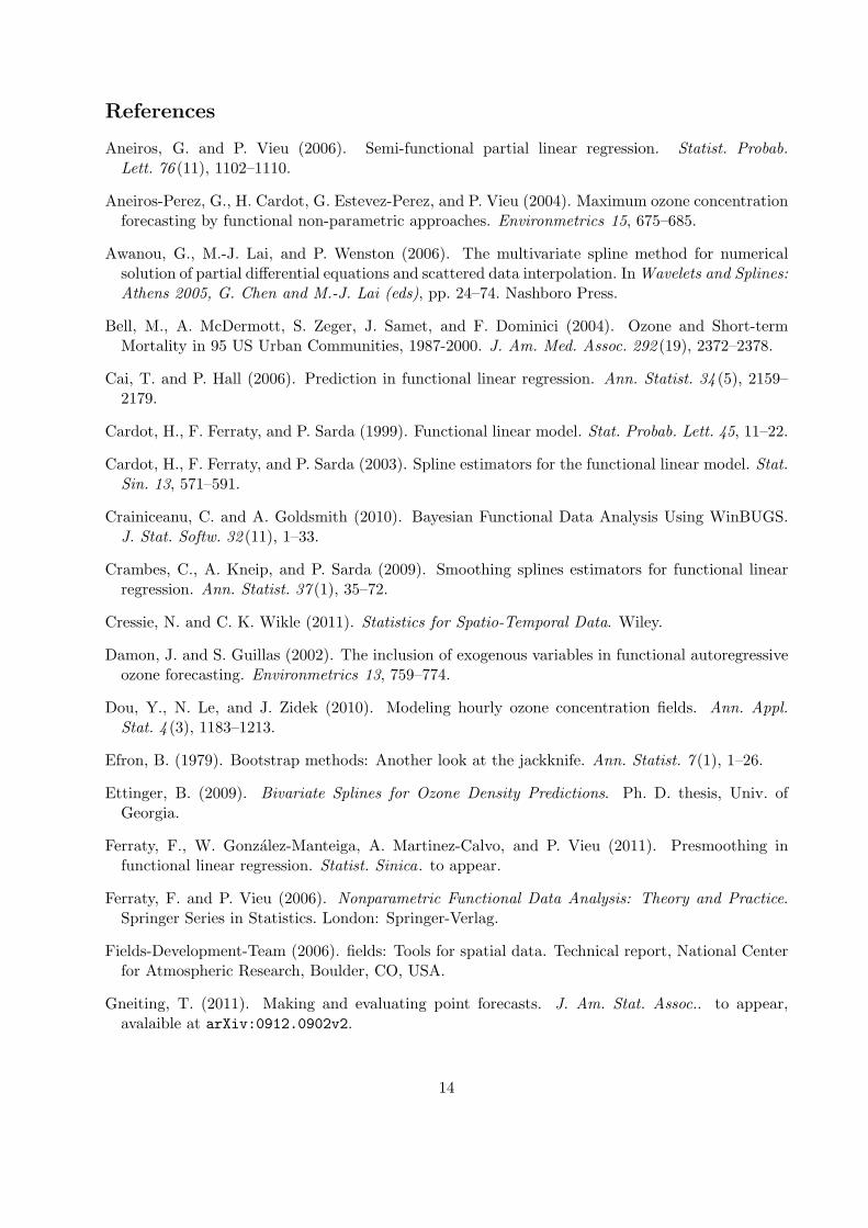
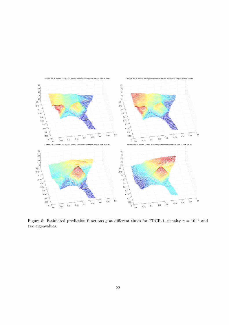
In this paper, we forecast the ground-level ozone concentration at one EPA station in suburbanAtlanta (in Kennesaw, GA, latitude 34.0138◦N, longitude 84.6049◦N) using the random surfacesover the entire U.S. domain based on the measurements at various EPA stations from the previousdays. The locations are scattered over a complicated domain, delimited by the United Statesfrontiers, which has been scaled into [0, 1]× [0, 1], see Figure 1.There are about 1000 EPA stations in the U.S. We are given the ozone concentrations at eachlocations for every hour over three months from July to September, 2005. The amount of themissing data is very small, so they affect very slightly our computations as the penalized leastsquares fit was used. Assume that the ozone concentration in a city, say Atlanta on one day at aparticular time is a linear functional of the ozone concentration distribution over the surroundingregion of the U.S. continent on the previous day. Also we may assume that the linear functional iscontinuous. Thus, we can use functional linear model for prediction.With bivariate spline functions, we can easily carry out all the experiments to approximate theozone distributed random surfaces and approximate the linear functional. Based on bivariatesplines theory, the smaller the triangulation size, the better the approximation. In the followingnumerical experiments, we considered three different sizes of triangulations over the South East ofthe USA, depicted in Figure 2.We first use BF, following (1), with penalty ρ = 10−9. This level of penalty was considered reason-able after some preliminary analysis. We could have formally searched for an optimal penalty ρ butit was relatively clear that a few orders of magnitude of potential ρ values would work well, so wekept ρ = 10−9. In that setting, f(X) is the ozone concentrations at the station of interest at oneparticular hour of one day and X is the ozone concentration distribution function over the SouthEast of the USA at the same hour, but on the previous day. We use a penalized least squares fitSX of X with penalty γ to compute the empirical estimate Sα,n.Let us explain our numerical procedures in detail. To forecast the ozone concentration on a par-ticular day, we build hourly surfaces for all hours over all days in the sample, before the day atwhich we want to predict. We have two options: one in which 24 functions Sg are estimated usingthe data Y and X for each hour of the day (BF-1), and one in which one function Sg is estimatedusing all hours of the day (BF-24). In the second option, the sample size is 24 times larger, but therelationship between the surface of ozone at an hour and ozone at the station 24 hours ahead doesnot depend on the hour. This stationarity assumption weakens BF-24 but enables the computationof more robust predictions when the number of days in the sample is small, and these methodssuffer from autocorrelation leakage for nearby hours. The same notations are adopted for FPCR-1and FPCR-24. The methods BF-1 and FPCR-1 do no suffer from autocorrelation leakage as moststudies show significant autocorrelation only over 2-3 hours for ground-level ozone, but use a muchsmaller sample size.For illustration of both BF and FPCR, we display in Figure 3 the 24 hour ahead predictions overtwo different days, based on length varying from 10 to 22 days of learning. The methods give similarresults, but FPCR seems to provide better forecasts than BF, with not as much of a need for alarge sample size to provide good predictions. In the next two sections we quantify the predictiveabilities of these two techniques.Figure 4 and 5 respectively display estimates for the prediction functions g for BF-1 and FPCR-1at four different times of the day (5AM, 11AM, 3PM and 6PM). The scales are different for BFand FPCR. Indeed, the empirical eigenvalues for FPCR are much larger here than for the matrix

9

An in BF, as we use polynomials without any smoothness condition across edges in a first step.The resulting eigenvectors that help us reconstitute the prediction functions g are therefore muchsmaller for BF.

3.1 BF predictions

Here we present numerical results using BF to predict at the Atlanta station. It is necessary tochoose the value of γ. Figure 6 displays the averaged daily RMSEs of predictions over August20-31, 2005 for various choices of γ, as well as averaged daily Mean Absolute Deviations (MAD)and averaged daily maximum error. It shows that RMSEs decrease rapidly with sample size andlevel off at around 20 observations. It also indicate that γ ought to not be chosen too large or toosmall, but its impact on the predictions is relatively minor for BF-24. For BF-1, it is necessary tochoose a high value for γ, here γ = 1, as too much roughness in the hourly surfaces X can producevariability on the estimates of the functions g due to a much smaller sample size.

3.2 FPCR predictions

We show our numerical results using our FPCR approach to predict at the Atlanta station. In thatsetting, it is necessary to choose a number of eigenvalues/eigenvectors to carry out the predictions.Hence we have one additional tuning parameter in addition to the γ values. Figures 8 and 9 displayRMSEs for one such choice of 2 eigenvalues according to sample size. It shows that for FPCR-24, RMSEs are already small for sample sizes of only 5 days, and decrease very slowly. It is aremarkable behaviour of this method to be able to learn with a very small number of days. ForFPCR-1, which uses 24 times less data points but exactly at the hour of interest, the RMSEs aremuch larger but decrease steadily from these large values and reach lower values than FPCR-1 afteraround 20 days. Hence FPCR-1 is more tailored to the problem, but requires more days.We considered 2, 4, 6 and 10 eigenvalues only, as forecasts were not improved by employing morethan 10 eigenvalues. The tables of RMSEs ranked by size of the learning period, for 2, 4, and6 eigenvalues, are not displayed here but show similar behavior. Table 1 summarizes RMSEs forthese various choices for FPCR-24 and provides a comparison with BF-24 for a sample size of 30days.Such RMSE calculations can provide the basis for cross-validation over a subset of days prior to theprediction period. However, one must be careful to choose the adequate performance criterion (e.g.RMSE, MAD) to match cross-validation and the forecasting task (Gneiting, 2011). We used RMSEin the sequel but paid attention to potential variations across performance criteria, see Figure 6.

4 Comparison with thin-plate splines

In this section, we assess the predictive abilities of BF using either bivariate splines or thin-platesplines. Thin-plate splines also minimize

∑Nk=1 |h(sk)−Xi(sk)|2 + γEn(h) and lead to solution in

a basis of thin-plate splines of the type:

h(x) =

n∑i=1

δiη(‖x− xi‖) +3∑

j=1

αjφj(x)

where φj are linearly independent polynomials of degree 2, and η(r) is proportional to r2 log(r)(radial functions), see Wood (2003) and references therein. We use here the R package fields

(Fields-Development-Team, 2006) to fit thin-plate splines. Figure 10 depicts the predictions for

10

September 10, with varying sample sizes, obtained using the BF with thin-plate splines (withpenalty gamma chosen by cross-validation) instead of bivariate splines. A lack of coherence inthe predictions across hours can be seen when small samples are used to predict. For instance,forecasts at 18:00, 19:00 and 20:00 dramatically differ for sample sizes of 10 and 14 days, anddampen for larger sample sizes. This phenomenon occurs systematically over the validation period.The explanation is that the lack of spatial fit, compared to bivariate splines, may deteriorate theinference when only limited information is available. We can quantify this variability through theuse of jackknife (Efron, 1979). For a day, we carry out predictions using 10 out of the 11 daysprevious to the day before predictions are made, removing one day at a time out of the sample,and we produce 10 predictions for the BF with either bivariate splines or thin-plate splines. Asshown in Figure 11, the resulting variability in the forecasts is much larger using thin-plate splinescompared to using bivariate splines.Table 2 shows that the BF-1 with bivariate splines (BF-BS-1) surpasses the BF-1 with thin-platesplines (BF-TPS-1) over the period September 5-14 (not overlapping the period September 1-4considered in the jackknife illustration above and showing similar behavior). It is so by a largemargin for small sample sizes and by a small margin for larger sample sizes. The BF with thin-platesplines needs at least 16 days of learning to give reasonable predictions, due to the aforementionedhigh sensitivity to the given sample. The decrease in RMSE is slow for 10-15 days and then abruptfrom 15 to 16. This pattern is reflected as well over one day in Figure 10 where we can observea sudden improvement in predictive power for the morning (mean level) as well as the afternoon(large reduction in variability); the possible explanation for such sensitivity may be the non-linearnature of the thin-plate splines fitting compared to bivariate splines fitting. Table 2 also shows theadvantage of using 24 hours when computing the estimate of g: one does not need a large numberof days to be able to produce reasonable predictions. However, the drawback of this feature is thatwhen sample size increases, the predictions are made using too much averaging, compared to thetailored 1-hour based version, as seen clearly when comparing the variation of RMSEs with samplesize for BF-BS-24 and BF-BS-1. To compensate for larger instability when using smaller samplesize in BF-BS-1 and FPCR-1, we increased the penalty up to γ = 1 to obtain good predictions.Thin-plate splines are globally supported, so large scale influences can occur in the fit with norespect of boundaries and sharp variations. Bivariate splines are locally supported, and can fit inany geometry of polygonal domain of interest. As a result, bivariate splines are more likely to betterrepresent local variations. Furthermore, the computational cost of using radial functions of the kindr2 log(r) is large due to numerical approximations in the integrals used to derive scalar products,whereas bivariate splines are merely polynomials for which immediate and exact results for integralscan be obtained. We noticed differences of several orders of magnitude in our particular computerset-up between bivariate splines and thin-plate splines. To overcome the difficulty of numericalapproximations, Reiss and Ogden (2010) used another basis of radial functions: radial cubic B-splines over compact domains for a neuroimaging application. However, these compactly supportedsplines do not possess optimal approximation properties, so their use may be restricted to samplelocations that are numerous and spatially covering the domain of interest, as in neuroimaging.

5 Comparison with the VAR model

In Table 2, we compare the performance of our functional approach with a standard multivariatetime series approach: the vector autoregression model (VAR). We use the the R package vars

(Pfaff, 2008) with the default settings. We first select each vector of EPA stations in the SouthEast at a selected hour. There are 210 locations in our data set, and fitting the VAR requires at

11

least 210 observations, so we cannot use a model for each hour of the day as for BF-1 and FPCR-1.Therefore we need to make use of all the previous hours in the 10-17 day samples to have enoughinformation to fit the VAR. To make a prediction using 10 days of learning for September 10, weare using a sample size of 240 hours, which is the same as in the BF/FPCR-24 models.The next challenge in employing the VAR model is to impute a few missing data. To do so, we useeither the spatial average over all available stations at the time when the observation is missing orthe average value over all available observations at the same hour and at the same location wherethe data is missing. We denote these methods VAR-space and VAR-time in Table 2. Note thatbivariate spline methods do not suffer from these imputation problem as they naturally include anexcellent interpolation step. We could have employed this step in the VAR-space to impute thesefew missing values but this was unlikely to significantly change the VAR predictions and we stickedto the standard VAR approach. Finally, because observations are rounded to the next integer bythe EPA, many of the columns in the observations are collinear, so we add negligible normallydistributed random numbers with mean zero and standard deviation 0.01 to each observation tomake the system solvable (correcting any values that becomes negative). The VAR models havehuge errors for the 10 day sample size because the system is nearly collinear. However, we do seea decrease in errors as the sample size increases. Nevertheless, both VAR approaches yield RMSEsaround 40-100% higher than the BF and FPCR for the maximum sample size of 17 days consideredhere.

6 Effect of triangulation

Unsurprisingly, preliminary analysis showed that large scale triangulations (such as the entire con-tinental USA) do not produce good forecasts as these spatial scales are producing spurious effects.Indeed, the chemistry and transport occur only at a regional scale on the 24 hour-ahead horizon.Hence, we only considered triangulations (see Figure 2) over the South-East USA to carry out sta-tistical inference. We were not able to draw a conclusion in terms of which one is the best as noneof these three triangulations is consistently better than the others across the days of the validationperiod. Obviously, there is an infinite number of triangulations for this region. Finding an optimaltriangulation for our purpose is very interesting and could lead to even better predictive abilities.It seems to be better to use a triangulation dependent on the geography as one wants to borrowstrength spatially in a meaningful manner. For example, the ridges of mountains should be edges ofthe triangulation; cities should be taken into account as predictions, for instance by putting themat the vertices of the triangulation. This investigation is beyond the scope of this paper.

7 Conclusions and Future Research

The BF method works very well for Atlanta. The predictions are consistent for various learningperiods and the predictions are close to the exact measurements. Using the first two eigenvaluesor more, FPCR also works very well. It is hard to say which one is better in general. However, onaverage, FPCR seems to slightly outperform BF in our example as it requires a smaller sample sizeto be efficient.Overall, we recommend BF since it is simpler than FPCR which requires some expert knowledgeabout how many eigenvalues are needed for the best prediction. In our examples, we observed thedecay of the eigenvalues, and often could not find an abrupt fall, also called a knee, if the values ofall eigenvalues are plotted a normal scale. When plotted on a logarithmic scale, each of eigenvalues(in the first 10 of them) has a knee. It is hard to decide which one is the right knee. Determination

12

of how many eigenvalues for the best prediction is not an easy task and requires further study. Yuanand Cai (2010) showed not only that the FPCR requires additional assumptions to be valid, but thaton well-designed simulations, predictions given by BF, with penalty ρ chosen with cross-validation,compares favorably to the FPCR from Hall and Horowitz (2007). However, if one has informationabout the principal components, or if the situation is made easy for their estimation, it may bepossible for FPCR to outperform BF in these cases. A reasonably accurate estimation of principalcomponents might explain why this occurred in our example over the prediction period September5-14. Finally, Ferraty et al. (2011) considered pre-smoothing for FPCR, that is the perturbationof the normal equation Γg = ∆ at the beginning of the analysis. It seems to significantly improvethe FPCR when the sample size is small or the noise is large. One could expect our results to beenhanced accordingly with the use of presmoothing.It is also interesting to study the ozone value prediction at other cities, e.g., Boston, Cincinnatiand others, see Ettinger (2009) for more details. The numerical results again show that BF is easyto use and performs well. We see that the quality of predictions reaches a plateau after a learningperiod of around 15 days. Although in theory we can predict better if we use a longer learningperiod, the numerical results vary based on our experiments. We also conducted experiments forpredictions using bivariate splines of degree d bigger than 5: we employed d = 6, 7, 8 and 9 (notreported here). The numerical results are broadly similar to the predictions using bivariate splinesof degree d = 5.The inclusion of co-variates (e.g. meteorological or even chemistry-transport model predictions) canimprove such purely statistical ozone predictions (Damon and Guillas, 2002; Guillas et al., 2008).We showed here the abilities of our method with no covariates, with potential gains from the use ofthis additional information. However, the treatment of covariates (themselves spatially distributed)in this spatial functional data context is challenging. One possibility is first to merely add a non-spatially varying average effect as a parametric component. Such semiparametric functional modelsare now well understood (Aneiros and Vieu, 2006). A better idea would be to fully integratethe functional covariates. Modelling and computational issues arise, and this is currently underinvestigation.Crainiceanu and Goldsmith (2010) recently developed Bayesian approaches for functional data,including a specific treatment of FPCR. Uncertainties are naturally computed as a result. SuchBayesian methods would most probably improve the quantification of uncertainties.When the overall geographical coverage of triangulation is reasonably small (the coarseness isanother issue), the predictions are better for both BF and FPCR for our particular example.Indeed, one should restrict itself to regions for which the spatial variability, through chemistry andtransport, corresponds to the time scale of the prediction. As a result, larger regions, possiblythe entire continental US, may be appropriate for predictions at longer horizons when larger scaletransport is occuring. One can foresee adaptive triangulations that would suit particular conditions.The major conclusion from our results above is that bivariate splines outperform thin-plate splinesin this context both in precision and computing time, and would do even more when the domainshows further constraints such as mountains and sea-shore that have a large impact on chemistryand transport due to their local features. Such qualities are attractive in various settings wheretaking boundaries into account would help improve interpolation over thin-plate splines (Newlandset al., 2011). We believe that our method has the potential to be implemented for operationalpollution forecasting as a result.

13

References

Aneiros, G. and P. Vieu (2006). Semi-functional partial linear regression. Statist. Probab.Lett. 76 (11), 1102–1110.

Aneiros-Perez, G., H. Cardot, G. Estevez-Perez, and P. Vieu (2004). Maximum ozone concentrationforecasting by functional non-parametric approaches. Environmetrics 15, 675–685.

Awanou, G., M.-J. Lai, and P. Wenston (2006). The multivariate spline method for numericalsolution of partial differential equations and scattered data interpolation. InWavelets and Splines:Athens 2005, G. Chen and M.-J. Lai (eds), pp. 24–74. Nashboro Press.

Bell, M., A. McDermott, S. Zeger, J. Samet, and F. Dominici (2004). Ozone and Short-termMortality in 95 US Urban Communities, 1987-2000. J. Am. Med. Assoc. 292 (19), 2372–2378.

Cai, T. and P. Hall (2006). Prediction in functional linear regression. Ann. Statist. 34 (5), 2159–2179.

Cardot, H., F. Ferraty, and P. Sarda (1999). Functional linear model. Stat. Probab. Lett. 45, 11–22.

Cardot, H., F. Ferraty, and P. Sarda (2003). Spline estimators for the functional linear model. Stat.Sin. 13, 571–591.

Crainiceanu, C. and A. Goldsmith (2010). Bayesian Functional Data Analysis Using WinBUGS.J. Stat. Softw. 32 (11), 1–33.

Crambes, C., A. Kneip, and P. Sarda (2009). Smoothing splines estimators for functional linearregression. Ann. Statist. 37 (1), 35–72.

Cressie, N. and C. K. Wikle (2011). Statistics for Spatio-Temporal Data. Wiley.

Damon, J. and S. Guillas (2002). The inclusion of exogenous variables in functional autoregressiveozone forecasting. Environmetrics 13, 759–774.

Dou, Y., N. Le, and J. Zidek (2010). Modeling hourly ozone concentration fields. Ann. Appl.Stat. 4 (3), 1183–1213.

Efron, B. (1979). Bootstrap methods: Another look at the jackknife. Ann. Statist. 7 (1), 1–26.

Ettinger, B. (2009). Bivariate Splines for Ozone Density Predictions. Ph. D. thesis, Univ. ofGeorgia.

Ferraty, F., W. Gonzalez-Manteiga, A. Martinez-Calvo, and P. Vieu (2011). Presmoothing infunctional linear regression. Statist. Sinica. to appear.

Ferraty, F. and P. Vieu (2006). Nonparametric Functional Data Analysis: Theory and Practice.Springer Series in Statistics. London: Springer-Verlag.

Fields-Development-Team (2006). fields: Tools for spatial data. Technical report, National Centerfor Atmospheric Research, Boulder, CO, USA.

Gneiting, T. (2011). Making and evaluating point forecasts. J. Am. Stat. Assoc.. to appear,avalaible at arXiv:0912.0902v2.

14

Guillas, S., J. Bao, Y. Choi, and Y. Wang (2008). Statistical correction and downscaling of chemicaltransport model ozone forecasts over Atlanta. Atmospheric Environment 42, 1338–1348.

Guillas, S. and M. Lai (2010). Bivariate splines for spatial functional regression models. J. Non-parametric Stat. 22 (4), 477–497.

Hall, P. and J. Horowitz (2007). Methodology and convergence rates for functional linear regression.Ann. Statist. 35 (1), 70–91.

Lai, M.-J. (2008). Multivariate splines for data fitting and approximation. In Approximation TheoryXII: San Antonio 2007, M. Neamtu and L. L. Schumaker (eds.), pp. 210–228. Nashboro Press.

Lai, M.-J. and L. Schumaker (2007). Spline Functions over Triangulations. Cambridge UniversityPress.

Neidell, M. (2010). Air quality warnings and outdoor activities: evidence from Southern Californiausing a regression discontinuity design. J. Epidemiol Community Health 64 (10), 921–926.

Newlands, N. K., A. Davidson, A. Howard, and H. Hill (2011). Validation and inter-comparison ofthree methodologies for interpolating daily precipitation and temperature across canada. Envi-ronmetrics 22 (2), 205–223.

Paciorek, C. J., J. D. Yanosky, R. C. Puett, F. Laden, and H. H. Suh (2009). Practical large-scalespatio-temporal modeling of particulate matter concentrations. Ann. Appl. Stat. 3 (1), 370–397.

Pfaff, B. (2008). Var, svar and svec models: Implementation within R package vars. Journal ofStatistical Software 27 (4).

Ramsay, J. and B. Silverman (2005). Functional Data Analysis. Springer-Verlag.

Reiss, P. and R. Ogden (2010). Functional Generalized Linear Models with Images as Predictors.Biometrics 66 (1), 61–69.

Wood, S. N. (2003). Thin plate regression splines. J. R. Stat. Soc. Ser. B Stat. Methodol. 65 (1),95–114.

Yuan, C. and T. Cai (2010). A reproducing kernel Hilbert space approach to functional linearregression. Ann. Stat. 38 (6), 3412–3444.

15

Tables and Figures

16

10−1 10−2 10−3 10−4 10−5 10−6 10−7 10−8

2 11.61 11.42 11.34 11.35 11.25 11.40 12.40 14.92

4 11.60 11.21 11.21 11.35 11.46 11.68 12.07 14.28

6 12.03 11.23 11.22 11.51 11.29 11.58 12.10 12.97

10 12.77 11.23 11.36 11.46 11.24 11.68 12.24 12.23

BF 11.33 11.20 11.03 10.87 11.00 10.86 10.84 11.57

Table 1: Average 30 Day RMSE over August 20-31 by γ values. FPCR-24 for 2, 4, 6 and 10eigenvalues, BF-24 for ρ = 10−9.

BF-TPS-1 BF-BS-24 BF-BS-1 FPCR-24 FPCR-1 VAR-space VAR-time10 19.75 13.68 14.58 9.82 10.08 3.07× 108 4.87× 109

11 19.46 13.58 13.61 9.91 9.98 50.78 111.7312 19.21 13.22 12.70 9.91 9.94 33.18 37.5413 18.76 13.03 12.12 9.90 9.99 27.70 28.3614 18.32 12.94 11.52 9.89 9.87 23.41 40.7815 18.36 13.15 11.30 9.91 9.74 18.80 23.1616 12.48 12.95 11.05 9.92 9.82 20.40 20.5117 12.08 12.55 10.98 9.85 9.80 19.79 17.77

Table 2: Average RMSEs of BF with thin-plate splines (BF-TPS), BF-24 with bivariate splines(γ = 10−4), BF-1 with bivariate splines (γ = 1), FPCR-24 with bivariate splines (γ = 10−4), FPCR-1 with bivariate splines (γ = 1), VAR-space, VAR-time, over Sept 5-14 (10 day-long validationperiod) with sample sizes from 10 to 17 days.

17

Figure 1: Locations of EPA stations and an example of a triangulation

18

Figure 2: Triangulations T1 (blue), T2 (red), T3 (black) of the South East of the USA.

19

2 4 6 8 10 12 14 16 18 20 22 240

10

20

30

40

50

60

70

80

90

100

hours

ozon

e(pp

b)

BF: Atlanta on Sept 7, 2005 on T1

True10 Day14 Day18 Day22 Day

2 4 6 8 10 12 14 16 18 20 22 240

10

20

30

40

50

60

70

80

90

100

hours

ozon

e(pp

b)

BF: Atlanta on Sept 10, 2005 on T1

True10 Day14 Day18 Day22 Day

2 4 6 8 10 12 14 16 18 20 22 240

10

20

30

40

50

60

70

80

90

100

hours

ozon

e(pp

b)

FPCR: Atlanta on Sept 7, 2005 on T1

True10 Day14 Day18 Day22 Day

2 4 6 8 10 12 14 16 18 20 22 240

10

20

30

40

50

60

70

80

90

100

hours

ozon

e(pp

b)

FPCR: Atlanta on Sept 10, 2005 on T1

True10 Day14 Day18 Day22 Day

Figure 3: Predictions using BF and FPCR with bivariate splines, over Sept. 7 and Sept. 10,with varying sample sizes for the learning periods prior to predictions, penalty γ = 10−4 for bothmethods and two eigenvalues for FPCR.

20

0.5 0.55 0.6 0.65 0.7 0.75 0.8 0.85 0.9

0

0.05

0.1

0.15

0.2

0.25

0.3

0.35

0.4

0.45

0.5

−1000

0

1000

2000

BF: Atlanta 33 Days of Learning Prediction Function for Sept 7, 2005 at 5 AM

0.5 0.55 0.6 0.65 0.7 0.75 0.8 0.85 0.9

0

0.05

0.1

0.15

0.2

0.25

0.3

0.35

0.4

0.45

0.5

−500

0

500

1000

1500

BF: Atlanta 33 Days of Learning Prediction Function for Sept 7, 2005 at 11 AM

0.5 0.55 0.6 0.65 0.7 0.75 0.8 0.85 0.9

0

0.05

0.1

0.15

0.2

0.25

0.3

0.35

0.4

0.45

0.5

−400

−200

0

200

400

BF: Atlanta 33 Days of Learning Prediction Function for Sept 7, 2005 at 3 PM

0.5 0.55 0.6 0.65 0.7 0.75 0.8 0.85 0.9

0

0.05

0.1

0.15

0.2

0.25

0.3

0.35

0.4

0.45

0.5

−2000

−1000

0

1000

2000

BF: Atlanta 33 Days of Learning Prediction Function for Sept 7, 2005 at 6 PM

Figure 4: Estimated prediction functions g at different times for BF-1, penalty γ = 10−4

21

0.5 0.55 0.6 0.65 0.7 0.75 0.8 0.85 0.9

0

0.05

0.1

0.15

0.2

0.25

0.3

0.35

0.4

0.45

0.5

−10

0

10

20

30

Smooth FPCR: Atlanta 33 Days of Learning Prediction Function for Sept 7, 2005 at 5 AM

0.5 0.55 0.6 0.65 0.7 0.75 0.8 0.85 0.9

0

0.05

0.1

0.15

0.2

0.25

0.3

0.35

0.4

0.45

0.5

−10

0

10

20

30

Smooth FPCR: Atlanta 33 Days of Learning Prediction Function for Sept 7, 2005 at 11 AM

0.5 0.55 0.6 0.65 0.7 0.75 0.8 0.85 0.9

0

0.05

0.1

0.15

0.2

0.25

0.3

0.35

0.4

0.45

0.5

0

10

20

30

Smooth FPCR: Atlanta 33 Days of Learning Prediction Function for Sept 7, 2005 at 3 PM

0.5 0.55 0.6 0.65 0.7 0.75 0.8 0.85 0.9

0

0.05

0.1

0.15

0.2

0.25

0.3

0.35

0.4

0.45

0.5

−20

0

20

40

60

Smooth FPCR: Atlanta 33 Days of Learning Prediction Function for Sept 7, 2005 at 6 PM

Figure 5: Estimated prediction functions g at different times for FPCR-1, penalty γ = 10−4 andtwo eigenvalues.

22

5 10 15 20 25 3010.5

11

11.5

12

12.5

13

13.5

14

14.5

15BF−24 Average RMSE over August 20−31, 2005

Sample Size

Ave

rage

RM

SE

Err

or

10−1

10−2

10−3

10−4

10−5

10−6

10−7

10−8

5 10 15 20 25 304.5

5

5.5

6

6.5

7

7.5

Sample Size

Ave

rage

MA

D E

rror

BF−24 Average MAD over August 20−31, 2005

10−1

10−2

10−3

10−4

10−5

10−6

10−7

10−8

5 10 15 20 25 3020

22

24

26

28

30

32

34

Sample Size

Ave

rage

Max

imum

Err

or

BF−24 Average Maximum Error over August 20−31, 2005

10−1

10−2

10−3

10−4

10−5

10−6

10−7

10−8

Figure 6: BF-24: Averaged daily RMSE, MAD and maximum error over August 20-31, 2005.Sample Size varies from 5 days of learning to 30 days, and penalty for bivariate splines fitting γvaries in the range 10−1 to 10−8.

23

5 10 15 20 25 3010

15

20

25

30

35

40

45

50

55

60BF−1 Average RMSE over August 20−31, 2005

Sample Size

Ave

rage

RM

SE

Err

or

100

10−1

10−2

10−3

10−4

10−5

10−6

Figure 7: BF-1 Average RMSE over August 20-31, 2005. Sample Size varies from 5 days of learningto 30 days, and penalty for bivariate splines fitting γ varies in the range 100 to 10−6.

5 10 15 20 25 3011

11.5

12

12.5

13

13.5

14

14.5

15

15.5FPCR−24 Average RMSE over August 20−31, 2005

Sample Size

Ave

rage

RM

SE

Err

or

10−1

10−2

10−3

10−4

10−5

10−6

10−7

10−8

Figure 8: FPCR-24 average RMSE over August 20-31 and 2 Eigenvalues. Sample Size by γ values,with number of days for the training period between 5 and 30.

24

5 10 15 20 25 3010.5

11

11.5

12

12.5

13

13.5

14

14.5

15

15.5FPCR−1 Average RMSE over August 20−31, 2005

Sample Size

Ave

rage

RM

SE

Err

or

100

10−1

10−2

10−3

10−4

10−5

10−6

Figure 9: FPCR-1 average RMSE over August 20-31 and 2 Eigenvalues. Sample Size by γ values,with number of days for the training period between 5 and 30.

25

Figure 10: Prediction using BF with thin-plate spline (BF-TPS), over Sept 10, with varying samplesizes for the learning periods prior to predictions.

26

5 10 15 20

020

4060

8010

0

Sept 1 , sample size: 10

hour

ozon

e

5 10 15 20

020

4060

8010

0

Sept 2 , sample size: 10

hour

ozon

e

5 10 15 20

020

4060

8010

0

Sept 3 , sample size: 10

hour

ozon

e

5 10 15 20

020

4060

8010

0

Sept 4 , sample size: 10

hour

ozon

e

Figure 11: Brute force jackknife predictions (sample size 10, after leave one out of 11), with bivariatesplines (green), thin-plate splines (red) over September 1 to 4.

27