Bistatic Synthetic Aperture Radar - Defence Research …cradpdf.drdc-rddc.gc.ca/PDFS/unc87/p523308.pdf · · 2012-08-03Bistatic Synthetic Aperture Radar TIF ... Bistatic Synthetic

Bistatic Synthetic Aperture RadarTIF – Report (Phase I)

Christoph H. Gierull

Defence R&D Canada √ Ottawa TECHNICAL REPORT

DRDC Ottawa TR 2004-190 November 2004

Bistatic Synthetic Aperture RadarTIF – Report (Phase I)

Christoph H. Gierull

Defence R&D Canada – Ottawa

Technical Report

DRDC Ottawa TR 2004-190

November 2004

Her Majesty the Queen as represented by the Minister of National Defence, 2004

Sa majeste la reine, representee par le ministre de la Defense nationale, 2004

Abstract

This technical report presents theoretical and experimental results of phase I of theTechnology Investment Fund (TIF) project on low probability of intercept, that isbistatic SAR. In bistatic SAR, the transmitter and receiver are spatially separatedand hence, the risks of detection and localization are significantly reduced, i.e., itsvulnerability to jamming is reduced and its survivability significantly increased.Bistatic SAR images include information that is complementary to monostatic im-ages due to the different scattering mechanisms involved. Such information couldlead to the development of new techniques for automatic target recognition andclassification.

The project investigates the feasibility of bistatic SAR and identifies performancelimits through a trade-off analysis between radar parameters/geometry and achiev-able resolution. As the main result, conclusions are drawn regarding the bistaticobservation time and the subsequent imaging performance under different bistaticconfigurations, as well as the performance degradation due to severe oscillatorphase noise or jitter. The report also includes a description of a bistatic SAR sim-ulator, an implemented version of a time domain bistatic SAR processor, and theanalysis of existing experimental bistatic clutter data sets.

Resum e

Le present rapport technique donne les resultats theoriques et experimentaux de laphase I d’un projet mene dans le cadre du Fonds d’investissement technologique(FIT) sur la faible probabilite d’interception (FPI), c’est-a-dire le radara synthesed’ouverture (RSO) bistatique. Dans le RSO bistatique, l’emetteur et le recepteursont separes spatialement, ce qui reduit significativement les risques de detectionet de localisation, c’est-a-dire que la vulnerabilite du radar au brouillage est reduiteet sa surviabilite, fortement accrue. Les images de RSO bistatique comportent del’information qui vient completer les images de radar monostatique en raison desdiff erents mecanismes de diffusion en jeu. Cette information pourrait menera lamise au point de nouvelles techniques de reconnaissance et de classification auto-matiques des cibles.

Le projet comporte uneetude de faisabilite du RSO bistatique et en definit les li-mites de rendement par une analyse comparative entre les parametres et la geometriedu radar, d’une part, et la resolution realisable. Comme grand resultat, des conclu-sions sont tirees au sujet du temps d’observation du radar bistatique et l’obtention

DRDC Ottawa TR 2004-190 i

subsequente d’images en fonction de differentes configurations de radar bistatique,ainsi qu’au sujet de la degradation du rendementa cause de grave bruit de phased’oscillateur ou gigue. Le rapport comprend aussi une description d’un simulateurde RSO bistatique, une version mise en æuvre d’un processeur de RSO bistatiquetemporel et l’analyse des series de donnees disponibles de clutter de radar bistatiqueexperimental.

ii DRDC Ottawa TR 2004-190

Executive summary

In military environments, imaging based on monostatic synthetic aperture radar(SAR) is, due to its active illumination of the scene, easily detected and thus highlyvulnerable to electronic counter measures or even destruction. Use of a bistatic (ormulti-static) system, with its transmitter spatially separated from the ‘silent’ receiv-ing systems significantly reduces the risk of receiver detection and increases surviv-ability. In addition to low probability of intercept (LPI), such a bistatic SAR config-uration offers additional surveillance capabilities, such as complementary imagerydue to forward-scattering measurements. The proposed concept opens a wide fieldof future, related research and will even lead to different applications, like bistaticSAR in combination with ground moving target indication or topographic mapping.Even forward looking SAR becomes possible with bistatic configurations (impos-sible with monostatic systems) which might be exploited in landing aids for aircraftor obstruction warning devices in helicopters. This work could also serve as foun-dation of R&D in the field of covert radar detection and passive imaging, which alsoexploits bistatic geometry but uses a non-cooperative illuminator of opportunity.

The purpose of this Technology Investment Fund (TIF) project is to investigate thefeasibility and the limitations of a bistatic SAR system. This includes theoreticalstudy and simulation of optimum bistatic SAR configurations, the development ofrobust processing algorithms for imaging, and an experimental demonstration withthe upgraded airborne SpotSAR system and a specially constructed stationary re-ceiver.

This report presents a theoretical framework for performance analysis predictionfor any bistatic geometry with respect to the geometric and radiometric ground res-olution. It introduces analysis of the most promising configurations, including theirperformance limits and relevant problems, as well as the development and imple-mentation of a bistatic SAR simulator, which will be used to confirm the analysisand to test bistatic SAR processors. Finally, the report describes the successfulcoherent processing of two existing bistatic clutter data sets (space-borne and air-borne data) measured at the Air Force Research Laboratories (AFRL) in Rome, NYin 2002.

This research provides a deep level of understanding of the capabilities and difficul-ties associated with bi- and multistatic SAR concepts. This knowledge will, for in-stance, be essential to perform system design studies and accurate cost/performancetrade-off analyses of SBR designs in combination with airborne systems for futuremilitary SAR applications. The application of such concepts could significantlyenhance Canada’s surveillance capabilities in times of conflict by reducing vulner-ability to receiver jamming and to direct attack of the surveillance asset.

DRDC Ottawa TR 2004-190 iii

Presently, Canada is in the favourable situation of being able to collect data from na-tional assets including both space-borne sensors, RADARSAT-1 and soon RADAR-SAT-2, and experimental airborne SAR systems, such as DRDC’s SpotSAR or En-vironment Canada’s C-band SAR. This rather unique position offers the opportu-nity to test sophisticated new radar concepts using measured data gathered underrealistic military conditions.

Christoph H. Gierull; 2004; Bistatic Synthetic Aperture Radar; DRDC OttawaTR 2004-190; Defence R&D Canada – Ottawa.

iv DRDC Ottawa TR 2004-190

Sommaire

Dans les milieux militaires, l’imagerie fondee sur le radara synthese d’ouver-ture (RSO) monostatique est, en raison de l’illumination active de la scene, fa-cilement detectee et, par consequent, hautement vulnerable aux contre-mesureselectroniques ou memea la destruction. L’utilisation d’un systeme bistatique (oumultistatique), dont l’emetteur est spatialement separe des systemes de reception‘silencieux’, reduit significativement le risque de detection du recepteur et accroıtla surviabilite. Outre la faible probabilite d’interception (FPI), une telle configura-tion de RSO bistatique offre des capacites additionnelles de surveillance, commel’imagerie complementaire gracea des mesures de prodiffusion. Le concept pro-pose ouvre un vaste domaine de recherches connexes et menera memea differentesapplications, comme l’utilisation du RSO bistatique en conjonction avec la car-tographie topographique ou l’indication de cibles mobiles au sol. Meme le RSOa visualisation vers l’avant devient possible avec les configurations de radar bi-statique (impossible avec les systemes monostatiques), et il pourraitetre exploitecomme aidea l’atterrissage pour les dispositifs de detection d’obstacle ou d’aeronefa bord d’helicopteres. Ce travail pourrait aussi servir de fondementa la rechercheet developpement dans le domaine de la detection radar discrete et de l’imageriepassive, qui exploite aussi la geometrie bistatique, mais qui utilise un illuminateurde choix non cooperatif.

Le but du present projet mene dans le cadre du Fonds d’investissement technolo-gique (FIT) est l’etude de la faisabilite et des limites d’un systeme RSO bistatique,y compris la simulation et l’etude theorique de configurations optimales de RSObistatique, la mise au point de solides algorithmes de traitement d’imagerie et unedemonstration experimentale au moyen du systeme SpotSAR aeroporte ameliore etd’un recepteur stationnaire particulier.

Le present rapport donne un cadre theorique de predication d’analyse du rendementde n’importe quelle geometrie bistatique en ce qui concerne la resolution au solgeometrique et radiometrique. Il introduit l’analyse des configurations les plus pro-metteuses, y compris leurs limites de rendement et les problemes pertinents, ainsique le developpement et la mise en place d’un simulateur de RSO bistatique, quiserviraa confirmer l’analyse eta mettrea l’essai les processeurs de RSO bistatique.Enfin, le rapport decrit le traitement coherent reussi de deux series disponibles dedonnees de clutter bistatique (donnees spatiales et de vol) prisesa l’Air Force Re-search Laboratory (AFRL)a Rome (N.Y.) en 2002.

Cette recherche permet d’obtenir une comprehension en profondeur des capaciteset des difficultes associees aux concepts du ROS bistatique et multistatique. Cesconnaissances sont, par exemple, essentiellesa la conduite d’etudes de conceptionde systemes et d’analyses comparatives cots/rendement precises des conceptions

DRDC Ottawa TR 2004-190 v

du radar satellise (RS) en conjonction avec les systemes aeroportes en vue d’appli-cations militaires futures du RSO. L’application de ces concepts pourrait ameliorersignificativement les capacites de surveillance du Canada en periodes de conflit, enreduisant la vulnerabilite au brouillage des recepteurs et aux attaques directes desdispositifs de surveillance.

Le Canada se trouve actuellement dans une situation favorable,etant en mesurede recueillir des donneesa partir de dispositifs nationaux, y compris les deux cap-teurs spatiaux (RADARSAT-1 et bientt RADARSAT-2) et des systemes spatiauxexperimentaux (comme SporSAR de RDDC ou le RSO en bande C d’Environne-ment Canada). Cette position plutt unique offre la possibilite de mettrea l’essaide nouveaux concepts perfectionnes dans le domaine du radara l’aide de donneesmesurees recueillies dans des conditions militaires realistes.

Christoph H. Gierull; 2004; Radar a synthese d’ouverture bistatique; DRDC OttawaTR 2004-190; R & D pour la defense Canada – Ottawa.

vi DRDC Ottawa TR 2004-190

Table of contents

Abstract . . . . . . . . . . . . . . . . . . . . . . . . . . . . . . . . . . . . . i

Resume . . . . . . . . . . . . . . . . . . . . . . . . . . . . . . . . . . . . . i

Executive summary . . . . . . . . . . . . . . . . . . . . . . . . . . . . . . . iii

Sommaire . . . . . . . . . . . . . . . . . . . . . . . . . . . . . . . . . . . . v

Table of contents . . . . . . . . . . . . . . . . . . . . . . . . . . . . . . . . vii

List of figures . . . . . . . . . . . . . . . . . . . . . . . . . . . . . . . . . . x

List of tables . . . . . . . . . . . . . . . . . . . . . . . . . . . . . . . . . . . xiii

Acknowledgements . . . . . . . . . . . . . . . . . . . . . . . . . . . . . . . xiv

1 Introduction . . . . . . . . . . . . . . . . . . . . . . . . . . . . . . . 1

2 Bistatic SAR signal model . . . . . . . . . . . . . . . . . . . . . . . 4

2.1 Constant oscillator frequency offset . . . . . . . . . . . . . . 5

2.1.1 Time history . . . . . . . . . . . . . . . . . . . . . . . 5

2.1.2 Fast-time (range) processing . . . . . . . . . . . . . . 6

2.1.3 Slow-time (Doppler) processing . . . . . . . . . . . . 8

2.2 Linear oscillator frequency drift . . . . . . . . . . . . . . . . 11

2.2.1 Fast-time (range) processing . . . . . . . . . . . . . . 12

2.2.2 Slow-time (Doppler) processing . . . . . . . . . . . . 13

2.3 Random oscillator phase noise . . . . . . . . . . . . . . . . . 14

2.3.1 Wideband (white) phase noise . . . . . . . . . . . . . 15

2.3.2 Realistic (colored) oscillator phase noise . . . . . . . . 17

2.3.3 Comparison to monostatic case . . . . . . . . . . . . . 24

3 Bistatic observation time . . . . . . . . . . . . . . . . . . . . . . . . 26

DRDC Ottawa TR 2004-190 vii

4 Bistatic SAR performance analysis . . . . . . . . . . . . . . . . . . . 31

4.1 Preliminaries: Doppler-bandwidth, Doppler-gradient and thek-space . . . . . . . . . . . . . . . . . . . . . . . . . . . . . 31

4.2 Doppler-resolution . . . . . . . . . . . . . . . . . . . . . . . 33

4.2.1 Special cases . . . . . . . . . . . . . . . . . . . . . . 35

4.2.1.1 Monostatic with omnidirectional antennapattern . . . . . . . . . . . . . . . . . . . . 35

4.2.1.2 Monostatic stripmap with realisticantenna pattern . . . . . . . . . . . . . . . 35

4.2.1.3 Bistatic with omnidirectional antenna pattern 36

4.2.1.4 Bistatic stripmap with realistic antennapattern . . . . . . . . . . . . . . . . . . . . 36

4.2.1.5 Bistatic stripmap with realistic antennapattern and stationary receiver . . . . . . . 38

4.2.2 Ground plane . . . . . . . . . . . . . . . . . . . . . . 39

4.3 Range-resolution . . . . . . . . . . . . . . . . . . . . . . . . 40

4.3.1 Ground plane . . . . . . . . . . . . . . . . . . . . . . 41

4.3.2 Equivalent bistatic nadir hole . . . . . . . . . . . . . . 41

5 Bistatic SAR raw data simulation . . . . . . . . . . . . . . . . . . . . 44

6 Bistatic clutter experiments . . . . . . . . . . . . . . . . . . . . . . . 47

6.1 RADARSAT-1 as illuminator . . . . . . . . . . . . . . . . . . 48

6.2 Convair 580 as illuminator . . . . . . . . . . . . . . . . . . . 55

6.3 Measured phase noise characteristics . . . . . . . . . . . . . . 62

6.3.1 Rooftop-RADARSAT-1 experiment . . . . . . . . . . 62

6.3.2 Rooftop-Convair 580 experiment . . . . . . . . . . . . 63

7 Bistatic SAR processing . . . . . . . . . . . . . . . . . . . . . . . . 65

viii DRDC Ottawa TR 2004-190

8 Summary and outlook . . . . . . . . . . . . . . . . . . . . . . . . . . 68

References . . . . . . . . . . . . . . . . . . . . . . . . . . . . . . . . . . . . 70

Annexes . . . . . . . . . . . . . . . . . . . . . . . . . . . . . . . . . . . . . 75

A Mean and variance of the impulse response function in presence ofwhite oscillator jitter . . . . . . . . . . . . . . . . . . . . . . . . . . 75

B Standard deviation of phase noise for a finite observation time . . . . 77

C Least squares estimation of phase noise polynomial coefficients . . . . 80

D Coordinate system conventions . . . . . . . . . . . . . . . . . . . . . 83

D.1 Scene coordinate system . . . . . . . . . . . . . . . . . . . . 83

D.2 Platform coordinate system . . . . . . . . . . . . . . . . . . . 83

D.3 Antenna coordinate system . . . . . . . . . . . . . . . . . . . 83

E Angular transformation conventions . . . . . . . . . . . . . . . . . . 85

E.1 Euler rotation angles . . . . . . . . . . . . . . . . . . . . . . 85

E.2 Angular transformation . . . . . . . . . . . . . . . . . . . . . 86

E.3 Scene into platform coordinate system . . . . . . . . . . . . . 86

E.4 Platform into antenna coordinate system . . . . . . . . . . . . 87

F State vector of platforms at time origin . . . . . . . . . . . . . . . . . 89

G Bistatic SAR processing algorithm . . . . . . . . . . . . . . . . . . . 90

DRDC Ottawa TR 2004-190 ix

List of figures

1 Bistatic SAR geometry with constant velocity of each platform. . . . . 4

2 Illustration of the phase and time shifts of the received pulses. . . . . . 6

3 Illustration of integration interval for range-compression. . . . . . . . 7

4 Expected displacement after range and Doppler compression alongoscillator frequency offset, range displacement in pixels forT = 50 µs (solid), Doppler displacement forTs = 0.5 s (dashed)and Doppler displacement forTs = 10 s (dash-dotted). . . . . . . . . 11

5 Impulse response function in the presence of white phase noise withσ = 0.04 (blue) andσ = 0.16 (red). . . . . . . . . . . . . . . . . . . 17

6 IISLR of OSC’s oscillator for increasing synthetic aperture time,upper curve based on eq. (39), lower curve based on eq. (42). . . . . . 19

7 Ideal point spread function (black) along with ten realisationsincluding phase noise with spectral density in the right-hand columnof Table 3. . . . . . . . . . . . . . . . . . . . . . . . . . . . . . . . . 20

8 Mean values of the polynomial coefficients with correspondingthresholds versus synthetic aperture time. . . . . . . . . . . . . . . . 22

9 Probability that the polynomial coefficients are larger than therequired threshold. . . . . . . . . . . . . . . . . . . . . . . . . . . . 23

10 Regions of possible solutions for the bistatic observation time. . . . . . 28

11 Bistatic observation time of ground range scatterer in seconds.Stationary tower-receiver and airborne transmitter for varyingbistatic anglesΨ0,2. . . . . . . . . . . . . . . . . . . . . . . . . . . . 30

12 Bistatic observation time and ground Doppler resolution for theairborne transmitter and airborne receiver configuration listed inTable 6. . . . . . . . . . . . . . . . . . . . . . . . . . . . . . . . . . 39

13 Ground range resolution in meters for a stationary receiver and anairborne transmitter with varying bistatic anglesΦ0,2. . . . . . . . . . 42

14 Illustration of the equivalent bistatic nadir hole atr = r0. . . . . . . . 43

x DRDC Ottawa TR 2004-190

15 Real part and magnitude of simulated bistatic raw data for anairborne transmitter and stationary receiver configuration,Ψ0,2 = 90◦. 46

16 Stationary bistatic receiver antenna at AFRL in Rome, NY. . . . . . . 47

17 Bistatic geometry for the trial at Rome, NY on 28 Jan. 2002. Theunderlying map (≈ 60 km x 70 km) was generated by MapPointc©2003 Microsoft Corp.,c©2003 NavTech and GDT, Inc. . . . . . . . 48

18 SNR enhancement via spectral filtering in IF. . . . . . . . . . . . . . . 49

19 Compressed pulse sidelobe reduction via matched filter. . . . . . . . . 50

20 Range migration correction and Doppler processing of direct pathsignal. . . . . . . . . . . . . . . . . . . . . . . . . . . . . . . . . . . 51

21 Range migration corrected bistatic raw data field. . . . . . . . . . . . . 53

22 Range and Doppler compressed bistatic SAR data. . . . . . . . . . . . 54

23 Zoom into close-range around the receiver location. . . . . . . . . . . 55

24 Photograph and location of active radar calibrator (ARC) at the 1Nov. 2002 airborne trial, crosses) receiver and ARC locations,arrow) flight path. . . . . . . . . . . . . . . . . . . . . . . . . . . . . 56

25 Predicted bistatic observation time and ground range resolution forthe Convair-Rooftop trial on 1 Nov. 2002 . . . . . . . . . . . . . . . 57

26 Received chirp and direct path signals (magnitude and phase). . . . . . 58

27 Magnitude and phase of ARC-signal at 3 km range and magnitudesof ARC-peaks along range. . . . . . . . . . . . . . . . . . . . . . . . 59

28 Range migration corrected raw data in logarithmic scale. . . . . . . . . 59

29 Matched filter banks for the chirp rate and the linear phase coefficientbased on the ARC-signal in Fig. 27 (b). . . . . . . . . . . . . . . . . 60

30 Bistatic SAR image for the 1 Nov. 2002 airborne trial. . . . . . . . . . 61

31 Bistatic SAR image for the 1 Nov. 2002 airborne trial around ARClocation. . . . . . . . . . . . . . . . . . . . . . . . . . . . . . . . . . 61

32 Measured phase noise of Rooftop-RADARSAT-1 experiment andimpact on point spread function. . . . . . . . . . . . . . . . . . . . . 62

DRDC Ottawa TR 2004-190 xi

33 Measured phase noise of Rooftop-Convair 580 experiment andimpact on point spread function. . . . . . . . . . . . . . . . . . . . . 63

34 Power density spectrum of phase noise for Rooftop-Convair 580experiment. . . . . . . . . . . . . . . . . . . . . . . . . . . . . . . . 64

35 Illustration of a bistatic raw data field (right) showing threeindividual range trajectories for scatterer locations specified in theilluminated footprint on the ground (left). . . . . . . . . . . . . . . . 66

36 SAR image processed with algorithm one and overlayed equi-rangeand equi-Doppler lines for three strong scatterers. . . . . . . . . . . . 67

B.1 Realisation of phase noise with sliding window to estimate the rmsfor finite observation timeT . . . . . . . . . . . . . . . . . . . . . . . 77

E.1 Euler rotation angles. . . . . . . . . . . . . . . . . . . . . . . . . . . 85

E.2 Angular relation between scene and platform coordinate systems. . . . 87

E.3 Angular relation between platform and antenna coordinate systems. . . 87

xii DRDC Ottawa TR 2004-190

List of tables

1 Second order termT 2s ∆a for oscillator drifts . . . . . . . . . . . . . . 14

2 Degradation of ISLR due to phase noise. . . . . . . . . . . . . . . . . 16

3 Measured SSBs for three commercial oscillators. . . . . . . . . . . . 18

4 Airborne transmitter parameters. . . . . . . . . . . . . . . . . . . . . 28

5 Tower receiver parameters. . . . . . . . . . . . . . . . . . . . . . . . 29

6 Bistatic airborne-airborne configuration . . . . . . . . . . . . . . . . 38

7 Simulation parameters. . . . . . . . . . . . . . . . . . . . . . . . . . 46

8 System parameters for the bistatic clutter trial of 28 January 2002. . . 48

DRDC Ottawa TR 2004-190 xiii

Acknowledgements

The author would like to cordially thank Turkish naval Lieutenant Nilufen Cotuk,who was working at DRDC Ottawa for an extended period under the Canadian De-fence Research Fellowship program, for his assistance in programming the bistaticspace-based SAR simulator and developing the time domain SAR processor. I amalso very thankful for his support during flight trials and the stripping of the exper-imental data.

Further, I would like to express my gratitude to Canadian liaison officer Capt. MarkAubrey and our American colleagues at AFRL in Rome, NY for their excellentwork during the numerous TTRDP trials and their support in providing the bistaticclutter data sets.

xiv DRDC Ottawa TR 2004-190

1 Introduction

In military environments, monostatic synthetic aperture radar (SAR) is, due to itsactive illumination of the scene, easily detected and thus highly vulnerable to elec-tronic counter measures or even destruction. Use of a bistatic/multi-static system,with its transmitter spatially separated from the ‘silent’ receiving systems signifi-cantly reduces the risk of receiver detection and increases survivability. Potentiallyqualified candidates for the transmitter are space based radars (SBR) or aircraftsflying at high altitudes. The receivers can be mounted on highly maneuverable air-craft or UAVs that may image the scene at different times and from different angles.In addition to low probability of detection, such a bistatic/multistatic SAR config-uration offers additional surveillance capabilities, such as complementary imagerydue to forward-scattering measurements. This may lead to the development of newtechniques for automatic target recognition and classification and could enhancethe visibility of stealthy targets. Furthermore, improved ground moving target in-dication (GMTI) and topographical surveying and mapping of the scene becomepossible.

Recently, there has been a growing interest in the use of space-based radars (SBR)to support the future military requirements of Canada and its allies. These require-ments include 24/7 wide-area surveillance of land targets under all weather condi-tions. Consequently, future military SBR systems will be equipped with syntheticaperture radar. Wide area coverage from space by SAR requires resolution to betraded off with swath coverage. It is further limited by the antenna power handlingcapacity, limited down-link capacity, lower SNR (due to larger distances betweensensor and targets) and a less flexible imaging geometry compared to airborne SARsystems. On the other hand, airborne SAR is highly vulnerable because, as an activesystem, its transmitted energy can be detected and hence intercepted, particularlywhen operating in a hostile environment. Interception includes active receiver jam-ming as well as the actual destruction of the radar platform.

This vulnerability may be overcome during a conflict by using a bistatic ‘low prob-ability of intercept’ SAR concept, where the radar transmitter may be located ona satellite, while the receiver is located on an airborne platform, such as a UAV.Since the receiving radar system operates in a passive (‘silent’) mode, the risk ofreceiver detection and localization is significantly reduced, i.e., its vulnerabilityto jamming is reduced and its survivability significantly increased. Compared tomonostatic space-based SAR, a higher SNR of the scattered echoes can also beachieved because of the smaller distances between the targets and the receiver. Fur-thermore, complementary information in the SAR images can be expected due tothe forward-scattering measurements of bistatic systems. For instance, the roofsof buildings might be the major source of scattering in bistatic SAR imagery com-

DRDC Ottawa TR 2004-190 1

pared to the walls in conventional, monostatic SAR images. Combined with theadvantages of a more flexible imaging geometry, it can be seen how such a bistaticSAR concept can enhance surveillance capabilities such as ground moving targetindication (GMTI) and topographical surveying and mapping.

In contrast to conventional, monostatic SAR, the required bistatic configuration hasa far more complex geometry that leads to certain unique problems that must bedealt with during image formation. Examples of such problems include greatervariation of Doppler frequency with range, non-linear Doppler frequency modula-tion in the along-track direction, reception of transmitter antenna mainlobe energythrough receiver antenna sidelobes, and fold-over effects resulting from range am-biguities. In order to generate high-resolution SAR images, the bistatic imaginggeometry must be known very accurately. This makes great demands on both themotion measurement system/equipment, such as INS and GPS, and the SAR signalprocessing/autofocus algorithms. Furthermore, the echo pulses must be coherentlymeasured, i.e., the phase information of the transmitted pulse has to be preserved.Hence, the problem of time synchronization between the two systems must be re-solved because the transmitter and receiver are spatially separated.

Although the investigation and application of bistatic radar is by no means new[1, 2, 3, 4], there appears to be a resurgence caused by technological progressand military exigency, particularly for imaging radars. Based on a growing con-fidence of technological feasibility, economical affordability, and due to palpableadvantages of bistatic SAR for military applications worldwide, scientific activitieshave intensified recently. Until two years ago only a handful of papers were pub-lished in the open literature. At the international conference on Geoscience andRemote SenSing (IGARSS’03), several papers about bistatic SAR appeared. Oneyear later, at the European SAR Conference EUSAR’04, there were two full ses-sions dedicated to phenomenology and processing of bistatic and multistatic SARdata. While the interest in bistatic SAR was in the past mostly stamped by militaryadvantages, even civil applications are starting to be discussed [5, 6]. Furthermore,highly sophisticated bi- and multistatic space-borne system concepts are being in-vestigated for enhanced applications such as interferometry [7, 8, 9] and SAR/MTI[10, 11, 12]. A step even further ahead is the possibility of passive (or parasitic)SAR imaging, which also exploits a bistatic geometry but using a non-cooperativeilluminator of opportunity [13, 14, 15].

However, a thorough and complete theoretical performance analysis with regardto the maximal geometric resolution determined by the three-dimensional flightgeometry and the maximum observation time is noticeably absent from the bistaticSAR literature. Further, due to lack of necessity in monostatic SAR (with only onelocal oscillator (LO) for up- and down conversion of the signals) the radiometricdeterioration caused by the severe phase noise of two separate LOs has not been

2 DRDC Ottawa TR 2004-190

extensively investigated in the past.

This TIF-project is divided into two phases. In Phase I, the theoretical backgroundof bistatic SAR has been derived via stepwise mathematical modeling of the re-ceived echo signals. Simultaneously, a simulation tool and bistatic SAR processingalgorithms are developed to evaluate and demonstrate the performance of the newSAR processing concepts. A detailed investigation of bistatic SAR performance,like achievable geometric and radiometric resolution, has been performed over awide range of bistatic geometries and radar operating parameters. In Phase II of theproject, deeper insight into the functionality of a bistatic SAR system and the phys-ical properties of its SAR imagery will be gained with experimental measurementsconducted by DRDC Ottawa’s airborne SpotSAR radar system.


2 Bistatic SAR signal model

In this Section a bistatic SAR signal model is derived as well as the predicted SARprocessing degradation due to oscillator frequency mismatch between the two sep-arated transmit and receive local oscillators. The output signal from two ideallynon-drifting oscillators would be a pure sine wave of exactly identical frequency,but any real device, even the most stable, is disturbed by unavoidable processessuch as random noise and drifts due to aging and/or environmental effects.

The starting point for the analysis of bistatic SAR is the three-dimensional geometrydepicted in Fig. 1. While it was sufficient for investigation of bistatic radar in thepast to only consider two-dimensional geometries, analysis of bistatic SAR requiresa three-dimensional geometry, e.g., [16, 17]. As a convention in the remainder ofthis document, vector quantities are underlined and matrices are written in bold.The transpose operator is denoted as superscript ’, complex conjugate as * andcomplex conjugate transpose as the Hermitian operator†.

H1

R0,1

R r1(t, )

R r2(t, )

R0,2

xs

zs

ys

r

v2

v1

H2

v1tn

Figure 1 : Bistatic SAR geometry with constant velocity of each platform.

Consider two independent, spatially separated, radar platforms moving along straight


paths in the three-dimensional Cartesian scene co-ordinate system, which is de-noted by subscript s, appendix D.1. The two platforms are not necessarily requiredto be aircrafts. For example, using a satellite as illuminator is a particularly inter-esting configuration, as will be shown later.

A detailed definition and description of all involved co-ordinate systems is givenin appendix D. The center (origin) of the scene is defined as the intersection ofthe transmitter and receiver pointing vectors with the ground plane at timet = 0.We are assuming that both platforms are flying in a plane parallel to the groundplane, i.e., with constant altitudesHi and with constant velocitiesvi for i = 1, 2.These assumptions are not restrictive and are only made to clarify the followingderivations.

The range vector from the transmitter (henceforth denotes by subscript1) to a pointr on the ground at timet is given as

R1(t, r) =(R0,1 − r

)+ v1t, (1)

whereR0,1 = R1(0, 0) is the vector from the scene center to the transmitter at timezero, see appendix F. This vector is commonly determined by the depression an-gle in elevation and the squint angle in azimuth at the time origin, see appendixA. Analogously, the range vector for the receiver is denoted by subscript2. Notethat the subscripts 1,2 are used rather than, e.g., ‘t,r’ to indicate the complete inter-changeability of receiver and transmitter, from a physical model point-of-view.

2.1 Constant oscillator frequency offset2.1.1 Time history

At subsequent instances in time, denoted bytn = n∆T for n = 0, 1, 2, . . ., thetransmitter coherently radiates a linear frequency modulated (LFM) pulse with car-rier frequencyω1 of form Re{strans(t)} with

strans(t) =∞∑

n=0

ejπ BT

(t−tn)2ej(ω1t+φ1(0)+ξ1(t)) rect

(t− tn

T

)+ n1(t), (2)

whereB is the chirp bandwidth,T is the pulse duration, and∆T is the pulse rep-etition interval (PRI). The termn1(t) represents unavoidable additive noise, e.g.,the thermal sensor noise in the transmitter hardware. It is usually modeled as astationary complex normal distributed stochastic process, i.e., a Gaussian processwith expectation zero and auto-covariance functioncn1n1(t). However, since we areat this point interested in phase noise effects, the additive noise term is omitted inthe following for didactical clarity. The stochastic processξ1(t) denotes the ‘multi-plicative’ phase noise, i.e., describes oscillator phase instabilities such as jitter. The


constant initial phaseφ1(0), at time origin, does not effect the SAR performanceand can be set to zero.

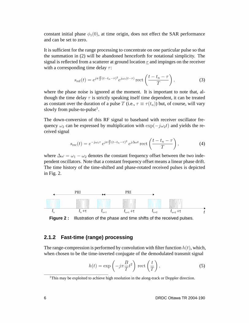
It is sufficient for the range processing to concentrate on one particular pulse so thatthe summation in (2) will be abandoned henceforth for notational simplicity. Thesignal is reflected from a scatterer at ground locationr and impinges on the receiverwith a corresponding time delayτ :

sref(t) = ejπ BT

(t−tn−τ)2ejω1(t−τ) rect

(t− tn − τ

T

), (3)

where the phase noise is ignored at the moment. It is important to note that, al-though the time delayτ is strictly speaking itself time dependent, it can be treatedas constant over the duration of a pulseT (i.e.,τ ≡ τ(tn)) but, of course, will varyslowly from pulse-to-pulse1.

The down-conversion of this RF signal to baseband with receiver oscillator fre-quencyω2 can be expressed by multiplication withexp(−jω2t) and yields the re-ceived signal

srec(t) = e−jω1τ ejπ BT

(t−tn−τ)2 ej∆ωt rect

(t− tn − τ

T

), (4)

where∆ω = ω1 − ω2 denotes the constant frequency offset between the two inde-pendent oscillators. Note that a constant frequency offset means a linear phase drift.The time history of the time-shifted and phase-rotated received pulses is depictedin Fig. 2.

tn

tn

+t tn+1

+t tn+2

+ttn+1

tn+2

PRI PRI

t

Figure 2 : Illustration of the phase and time shifts of the received pulses.

2.1.2 Fast-time (range) processing

The range-compression is performed by convolution with filter functionh(t), which,when chosen to be the time-inverted conjugate of the demodulated transmit signal

h(t) = exp

(−jπ

B

Tt2)

rect

(t

T

), (5)

1This may be exploited to achieve high resolution in the along-track or Doppler direction.


maximizes the signal-to-noise ratio (SNR). The matched filter output or impulseresponse function is given as

p(t) = (srec ? h)(t) =

∞∫−∞

srec(t′)h(t− t′)dt′ =

∞∫−∞

srec(t− t′)h(t′)dt′

= e−jω1τ

∞∫−∞

ejπ BT

(t−t′−tn−τ)2ej∆ω(t−t′)

·e−jπ BT

t′2 rect

(t− t′ − tn − τ

T

)rect

(t′

T

)dt′. (6)

The two rectangular functions within the integrand of (6) restrict the integrationinterval to the time-dependent valuesa(t) andb(t) (to be specified), that is:

p(t) = e−jω1τej∆ωt

b(t)∫a(t)

ejπ BT

((t−tn−τ)2−2(t−tn−τ)t′

)e−j∆ωt′dt′

= e−jω1τej∆ωtejπ BT

(t−tn−τ)2

b(t)∫a(t)

e−j(2π B

T(t−tn−τ)+∆ω

)t′dt′

= e−jω1τej∆ωtejπ BT

(t−tn−τ)2e−j(2π B

T(t−tn−τ)+∆ω

)b(t)+a(t)

2

· 2(b(t)− a(t)

)sinc

((2π

B

T(t− tn − τ) + ∆ω

)b(t)− a(t)

2

). (7)

The definition of the integration interval is illustrated in Fig. 3.

t’tt-t -

nJ t + -T

nJ t + +

nJ Tt +

nJ

T/2

T

-T/2 T/2

T

0

b(t)-a(t)

Figure 3 : Illustration of integration interval for range-compression.

The integration intervalb(t) − a(t) is non-zero when the right rectangle starts totouch the left one at timet = tn + τ + T , is maximum when they are completelyoverlap att = tn + τ , and linearly decreases untilt = tn + τ − T . The triangulartime history can be expressed analytically as

b(t)− a(t) =(T − |t− tn − τ |

)rect

(t− tn − τ

2T

). (8)


The sum of the two limits can be expressed as

b(t) + a(t) = (t− tn − τ) rect

(t− tn − τ

2T

). (9)

From (8) it is clear that within the vicinity of the reflected pulsest = tn + τ the in-tegration region can be approximated by the constant pulse lengthT , as commonlydone in the literature:

p(t) ∼= 2Te−jω1τej∆ωtejπ BT

(t−tn−τ)2 sinc

((2π

B

T(t− tn − τ) + ∆ω

)T2

). (10)

The effect of an oscillator frequency mismatch becomes apparent, namely the posi-tion of the peak is displaced from the correct location. Setting the argument of thesinc-function in (10) to zero yields

t0 = tn + τ − T∆f

Bor B(t0 − tn − τ) = T∆f, (11)

where∆f = ∆ω/2π = f1 − f2. As the range resolution is determined by theinverse of the pulse bandwidth (τ0 = 1/B), the value ofB(t0 − tn − τ) = B∆τrepresents the range displacement in multiples of the resolution cell size.

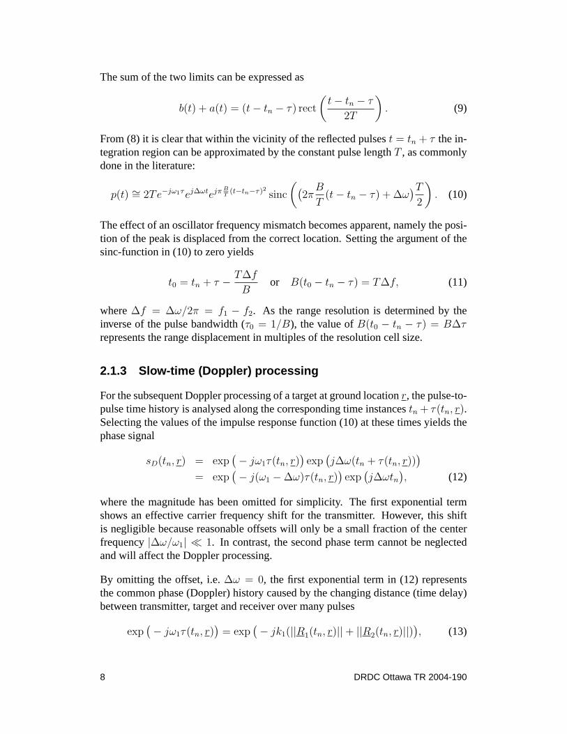
2.1.3 Slow-time (Doppler) processing

For the subsequent Doppler processing of a target at ground locationr, the pulse-to-pulse time history is analysed along the corresponding time instancestn + τ(tn, r).Selecting the values of the impulse response function (10) at these times yields thephase signal

sD(tn, r) = exp(− jω1τ(tn, r)

)exp

(j∆ω(tn + τ(tn, r))

)= exp

(− j(ω1 −∆ω)τ(tn, r)

)exp

(j∆ωtn

), (12)

where the magnitude has been omitted for simplicity. The first exponential termshows an effective carrier frequency shift for the transmitter. However, this shiftis negligible because reasonable offsets will only be a small fraction of the centerfrequency|∆ω/ω1| � 1. In contrast, the second phase term cannot be neglectedand will affect the Doppler processing.

By omitting the offset, i.e.∆ω = 0, the first exponential term in (12) representsthe common phase (Doppler) history caused by the changing distance (time delay)between transmitter, target and receiver over many pulses

exp(− jω1τ(tn, r)

)= exp

(− jk1(||R1(tn, r)||+ ||R2(tn, r)||)

), (13)


wherek1 = 2πf1/c denotes the transmitted wavenumber. To get deeper insight,it is sufficient now to consider a quasi-monostatic geometry with an approximatequadratic range-time history. It will be shown later that such scenarios comprisebistatic flight geometries with parallel paths of both platforms as well as either astationary transmitter or receiver. For a conventional monostatic SAR with identi-cal distances, equation (13) yields the classic Doppler phase history (second orderTaylor series):

φ(t, r) = 2k1||R(t, r)|| ∼= 2k1

(Rb(r) +

v2a

2Rb(r)(t− tb)

2

), (14)

where, for notational simplicity, the slow-timetn has been replaced byt andk1 byk. This convention will be used henceforth when possible without confusion. Thetime where the platform is broadside to the scatterer located atr is denoted bytband the distance between them (at this instant in time) byRb. For non-squintedSAR geometries and stationary reflectors, the timetb coincides with the point ofclosest approach [18].

Inserting (14) into (12) yields the slow-time or Doppler signal that can be writtenas

sD(t, r) = exp

(−j2k

(Rb(r)−

∆ω

2ktb

))· exp

(j2k

(∆ω

2k(t− tb)−

v2a

2Rb(r)(t− tb)

2

)), (15)

where constant terms will be omitted from here onwards. The linear coefficientis tantamount to a quasi radial velocityvr = ∆ω/(2k). Analogously to the range-compression, the Doppler signal is convolved with the expected signal of a reflectorat locationtb = 0 (reference function):

pD(t, r) = (sD ? sref)(t) =

∞∫−∞

sD(t− t′)sref(t′) dt′, (16)

where

sref(t, r) = exp

(j2k

v2a

2Rb(r)t2)

rect

(t

Ts

), (17)

whereTs denotes the synthetic aperture time over which the particular reflector isobserved by the radar. The maximum duration that the reflector is in the antennabeamwidth is usually expressed by the antenna beamwidthθ3dB and the slant rangedistanceTs = θ3dBRb(r)/va. Using this value, the point spread function reads

pD(t, r) = ej2k

(∆ω2k

t− v2a

2Rb(r)(t−tb)

2

) Ts/2∫−Ts/2

e−j2k

(∆ω2k− v2

aRb(r)

(t−tb)

)t′

dt′


= 2Tsej2k

(∆ω2k

t− v2a

2Rb(r)(t−tb)

2

)sinc

(k

(∆ω

2k− v2

a

Rb(r)(t− tb)

)Ts

).

(18)

Again, the peak is displaced by∆tb = (t′b − tb), wheret′b is computed by settingthe argument of the sinc-function to zero

t′b = tb +∆ωRb(r)

kv2a

or ∆tb = (t′b − tb) =λRb(r)

v2a

∆f. (19)

The displacement in meters is given byva∆tb. Normalizing this value to the wellknown optimum azimuth or Doppler resolutionA/2, whereA ∼= λ/θ3dB denotesthe real aperture of the radar, yields the displacement in resolution cells

va(t′b − tb)

λ/(2θ3dB)=

2θ3dBRb(r)∆f

va

= 2Ts∆f. (20)

Bearing in mind that the synthetic aperture time is much larger than the pulse du-rationT , the displacement is seen to be much more severe in the Doppler-direction(cf. (11)).

Fig. 4 illustrates the different displacements for range and Doppler-direction aswell as for typical airborne and spaceborne parameters. The pulse duration foreither case was assumed to beT = 50 µs. From the solid curve in Fig. 4, a targetbecomes shifted by exactly one range cell for a frequency mismatch of∆f = 20KHz. Therefore the range displacement will only be significant for a rather largediscrepancy of the two local oscillator frequencies. In contrast, the correspondingdisplacement in Doppler direction will be on the order of10, 000 to one millionpixels for this frequency offset.

If, for instance, a maximum shift of only one pixel is required, the disagreementbetween the oscillator frequencies must be smaller than0.1 Hz, which is highlyunrealistic. However, it is important to note that no de-focussing in either directionoccurs due to a constant frequency offset, see also [19].


100 101 102 103 104 10510−6

10−4

10−2

100

102

104

106

108

∆ f [Hz]

Dis

plac

emen

t Erro

r [pi

xels

]

range [T=50µs]Doppler (Space: Ts=0.5s)Doppler (Air: Ts=10s)

Figure 4 : Expected displacement after range and Doppler compression alongoscillator frequency offset, range displacement in pixels for T =50 µs (solid), Doppler displacement for Ts = 0.5 s (dashed) andDoppler displacement for Ts = 10 s (dash-dotted).

2.2 Linear oscillator frequency drift

In addition to a constant frequency offset, in practise real oscillators drift slowlyaway from their nominal center frequency, for instance, caused by environmentalchanges, such as temperature, pressure or magnetic fields. Modern oscillators com-monly compensate for such drifts by temperature compensation. A TemperatureCompensated Crystal Oscillator (TCXO) typically contains a temperature compen-sation network to sense the ambient temperature and pull the crystal frequency toprevent frequency drift over the temperature range. An Oven Controlled Crystal Os-cillator (OCXO) usually contains an oven block (with temperature sensor, heatingelement, oven circuitry, and insulation) to maintain a stable temperature. OCXOsoffer a great improvement in frequency stability compared to simple TCXOs. Al-though, these techniques usually greatly improve the performance, residual driftscan still cause errors, particularly in radar applications. In space-based across-trackinterferometry, for instance, very long orbital segments are usually analysed in or-der to generate digital elevation models of entire continents. Even the smallestclock drifts lead to measurable and compromising phase artifacts [9, 20].

The aim of this section is to investigate how frequency drift influences the per-formance of a bistatic SAR, particularly since the two oscillators are spatially sepa-rated. The carrier frequencies are assumed to drift linearly away from their nominalvalue by

ω1(t) = ω1 + a1t and ω2(t) = ω2 + a2t, (21)


where theai denote the change of rate of frequency or drift rates; the physical unitis rad/s. A linear frequency drift corresponds to a quadratic phase deviation.

The quality of oscillators is commonly specified by a dimensionless relative stabil-ity quantity ε = ∆f/f , e.g.,ε = 1 · 10−8 means a frequency deviation of 100 Hzfor a 10 GHz X-band oscillator. Typical drift rates are10 to 100 Hz/s for TCXOs,0.1 to 1 Hz/s for higher quality OCXOs, and smaller than 0.1 Hz/s for the highestquality oscillators [21].

2.2.1 Fast-time (range) processing

In order to study the influence of drift individually, the constant oscillator frequencyoffset is set to∆ω = 0, which means that the two oscillators may be perfectlysynchronized at one point in time, and then are ‘free-running’ afterwards.

Generalizing the received (and into baseband down-converted) signal in (4) to time-dependent oscillator frequency:

srec(t) = e−jω2(t)·t ejπ BT

(t−tn−τ)2 ejω1(t−τ)·(t−τ) rect

(t− tn − τ

T

), (22)

inserting (21) into (22) and applying the filter function (5), leads to a matched filterresponse (analogous to (6))

p(t) = e−jω1τ

T/2∫−T/2

ejπ BT

(t−t′−tn−τ)2eja1(t−t′−τ)2e−ja2(t−t′)2e−jπ BT

t′2 dt′, (23)

where the integration limits are restricted to one-half of the pulse duration, as in(10). Re-writing (23) yields

p(t) = e−jω1τejπ BT

(t−tn−τ)2eja1(t−τ)2e−ja2t2

·T/2∫

−T/2

e−2j(π BT

(t−tn−τ)+∆at−a1τ)t′ej∆at′2 dt′. (24)

Since the second order phase deviation is virtually always smaller thanπ/2 overthe pulse duration, i.e.,(a1 − a2)T

2 = ∆aT 2 � π/2, the termexp(j∆at′2) can beomitted in (24) and we get

p(t) = e−jω1τejπ BT

(t−tn−τ)2eja1(t−τ)2e−ja2t2

· sinc

((π

B

T(t− tn − τ) + ∆at− a1τ

)T

). (25)


Assuming no range-ambiguities, the round trip delayτ is restricted to lie withinthe pulse repetition intervalτ < PRI = 1/PRF and the third summand in theargument of the sinc-function can be omitted. The peak of the sinc-function occursat time

t′0 =πB(tn + τ)

πB + ∆aT, (26)

which is different from the error-free valuet0 = tn + τ by

∆t0 = t′0 − t0 = −∆aT (tn + τ)

πB + ∆aT∼= −∆aT

πBtn (27)

for largen. In other words, the peak position of the matched filter response in therange direction drifts very slowly away from the correct location over time. How-ever, this effect will only become significant for unreasonably long time periods.For instance, it would take more than one hour to drift one range cell (B∆t0 = 1)when using TCXOs, and about 100 hours when using OCXOs.

2.2.2 Slow-time (Doppler) processing

By omitting the drift (∆t0 = 0) in (27), i.e., by sampling the signal (25) at slow-timestn + τ yields the Doppler history

sD(tn) = e−jω1τeja1t2ne−ja2(tn+τ)2 ∼= e−jω1τej∆at2ne−j2a2tnτ , (28)

wherea2τ2 is negligibly small. Re-writing the time delayτ in (13) and (14) to

τ =2

c

(Rb +

v2a

2Rb

t2b

)− 2v2

a

cRb

tbt +v2

a

cRb

t2 ≡ s0 + s1t + s2t2, (29)

the Doppler signal in (28) becomes

sD(t) = e−j(ω1s1+2a2s0)te−j(ω1s2+2a2s1−∆a)t2e−j2a2s2t3 , (30)

where for notational simplicitytn was replaced byt and the constant term omitted.After application of the reference functionsref(t) = exp(jω1s2t

2) rect(t/Ts), thepoint spread function, cf. (18), yields

pD(t) =

Ts/2∫−Ts/2

e−j(ω1s1+2a2s0)(t−t′)e−j(ω1s2+2a2s1−∆a)(t−t′2)e−j2a2s2(t−t′)3ejω1s2t′2dt′

= e−j(ω1s1+2a2s0)te−j(ω1s2+2a2s1−∆a)t2e−j2a2s2t3

·Ts/2∫

−Ts/2

ej(ω1s1+2a2s0+2(ω1s2+2a2s1−∆a)t+6a2s2t2)t′

· ej(2a2s1−∆a+6a2s2t)t′2e−j2a2s2t′3 dt′. (31)

Two conditions must be fulfilled to obtain a sharply focussed point spread function:


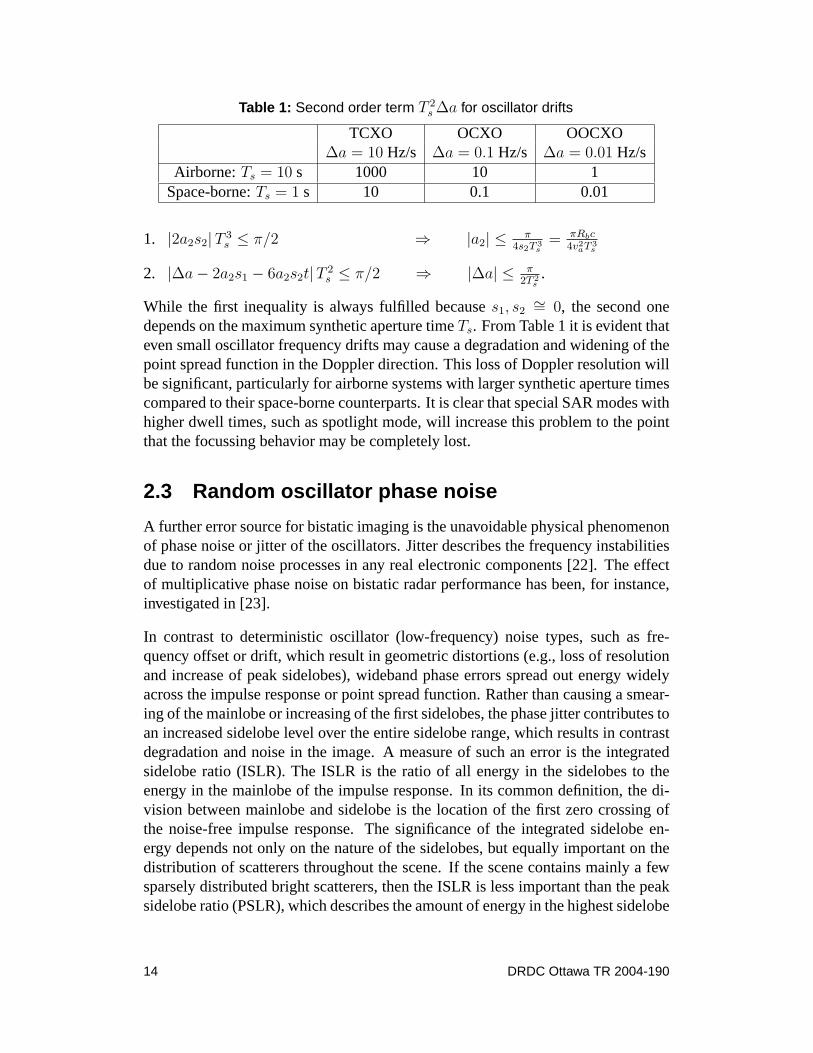
Table 1: Second order term T 2s ∆a for oscillator drifts

TCXO OCXO OOCXO∆a = 10 Hz/s ∆a = 0.1 Hz/s ∆a = 0.01 Hz/s

Airborne:Ts = 10 s 1000 10 1Space-borne:Ts = 1 s 10 0.1 0.01

1. |2a2s2|T 3s ≤ π/2 ⇒ |a2| ≤ π

4s2T 3s

= πRbc4v2

aT 3s

2. |∆a− 2a2s1 − 6a2s2t|T 2s ≤ π/2 ⇒ |∆a| ≤ π

2T 2s.

While the first inequality is always fulfilled becauses1, s2∼= 0, the second one

depends on the maximum synthetic aperture timeTs. From Table 1 it is evident thateven small oscillator frequency drifts may cause a degradation and widening of thepoint spread function in the Doppler direction. This loss of Doppler resolution willbe significant, particularly for airborne systems with larger synthetic aperture timescompared to their space-borne counterparts. It is clear that special SAR modes withhigher dwell times, such as spotlight mode, will increase this problem to the pointthat the focussing behavior may be completely lost.

2.3 Random oscillator phase noise

A further error source for bistatic imaging is the unavoidable physical phenomenonof phase noise or jitter of the oscillators. Jitter describes the frequency instabilitiesdue to random noise processes in any real electronic components [22]. The effectof multiplicative phase noise on bistatic radar performance has been, for instance,investigated in [23].

In contrast to deterministic oscillator (low-frequency) noise types, such as fre-quency offset or drift, which result in geometric distortions (e.g., loss of resolutionand increase of peak sidelobes), wideband phase errors spread out energy widelyacross the impulse response or point spread function. Rather than causing a smear-ing of the mainlobe or increasing of the first sidelobes, the phase jitter contributes toan increased sidelobe level over the entire sidelobe range, which results in contrastdegradation and noise in the image. A measure of such an error is the integratedsidelobe ratio (ISLR). The ISLR is the ratio of all energy in the sidelobes to theenergy in the mainlobe of the impulse response. In its common definition, the di-vision between mainlobe and sidelobe is the location of the first zero crossing ofthe noise-free impulse response. The significance of the integrated sidelobe en-ergy depends not only on the nature of the sidelobes, but equally important on thedistribution of scatterers throughout the scene. If the scene contains mainly a fewsparsely distributed bright scatterers, then the ISLR is less important than the peaksidelobe ratio (PSLR), which describes the amount of energy in the highest sidelobe


compared to the mainlobe. High peak sidelobes appear as false targets and hinderdetection of closely located weaker targets. In contrast, a low ISLR is important forhomogeneous scenes with evenly distributed weaker scatterers, where a high ISLRwill degrade contrast by filling in low returns and shadow areas [24].

2.3.1 Wideband (white) phase noise

In order to quantify the resulting ISLR for bistatic SAR, we start with the com-pressed pulse (23), where the drift terms are replaced by the corresponding phasenoise componentsξ1(t) andξ2(t) (cf. also (2))

P (t) = e−jω1τ 1

T

T/2∫−T/2

ejπ BT

(t−t′−tn−τ)2ejΞ1(t−t′−τ)e−jΞ2(t−t′)e−jπ BT

t′2 dt′. (32)

The capital letters in (32) are used to distinguish stochastic processes from their cor-responding realisations. The phase noise terms are modeled as stationary stochasticGaussian processesΞ(t) with expectation zero and auto-covariance function

cΞiΞi(t) =

1

2π

∞∫−∞

CΞiΞi(ω) exp (jωt) dω with cΞiΞi

(0) = σ2i , (33)

whereCΞiΞi(ω) denotes the spectral density function or the power spectrum. The

spectral density function is an important performance measure which is usually sup-plied by the manufacturer of oscillators. For a conventional monostatic SAR wherethe same oscillator is used for up- and down-conversion,Ξ2 equalsΞ1 (cf. section2.3.3), whereas in the bistatic case, two independent oscillators are used. Hence,Ξ2 andΞ1 are statisticallyindependent. More details and background informationabout the statistical frequency characteristics of precision clocks and oscillatorscan, for instance, be found in [22, 25, 26].

As a function of two random processes, the impulse response function (32) is againa stochastic process. For statistically white phase noise, its statistical propertieshave been determined in terms of the expectation function

EP (t) = e−σ21+σ2

22 e−jω1τejπ B

T(t−tn−τ) sinc (πB(t− tn − τ)) (34)

and the second moment function

E |P (t)|2 =√

2

(1− e−(σ2

1+σ22))

T+ e−(σ2

1+σ22) sinc2 (πB(t− tn − τ)) (35)


Table 2: Degradation of ISLR due to phase noise.

IISLR [dB] σ [rad]

-5 0.56-10 0.32-15 0.18-20 0.10-25 0.056-30 0.032

in appendix A. Therefore, the variance ofP (t) can be computed as

σ2p(t) = E |P (t)|2 − |EP (t)|2 =

√2

T

(1− e−(σ2

1+σ22))

, (36)

which denotes the power of the random part of the stochastic impulse response, andtherewith can be used to determine the sidelobe power levels caused by the phasejitter.

Integrating (36) over the entire pulse widthT , and usingexp(−σ2) ≈ 1 − σ2 forsmall phase noise terms, it becomes evident that the power level is raised over theentire compressed pulse length by the sum of the two phase noise variances. Hence,the increase (i.e., degradation) of the ISLR (IISLR) compared to the undisturbed orphase noise-free case is

IISLR =√

2(σ21 + σ2

2) =√

2

∞∫−∞

CΞ1Ξ1(f) + CΞ2Ξ2(f) df = 4√

2

∞∫0

CΞΞ(f) df,

(37)

where it was assumed that identical oscillator types withσ21 = σ2

2 are used. Theabove analysis is analogously applicable to the Doppler direction, where the pulseparameters in (32) are replaced by the Doppler rate in (17), and the pulse durationT is replaced by the synthetic aperture timeTs.

Table 2 lists the allowable phase noise, more specifically the constraint on the stan-dard deviation or root means square (rms) valueσ, in order not to exceed a certaindegradation in ISLR compared to the noise-free case. A maximum ISLR degrada-tion due to phase noise of IISLR= −20 dB is a typical requirement for imagingapplications [24].

To illustrate the impact of phase noise graphically, the red curve in Fig. 5 showsthe effect of aσ = 0.16 rms phase jitter (IISLR = -16 dB) on the impulse responsefunction in a bistatic scenario. In contrast, the case ofσ = 0.04 is plotted in blue(IISLR = -28 dB), which is virtually indistinguishable from the error-free case.


2.45 2.5 2.55 2.6 2.65

x 10−4

−70

−60

−50

−40

−30

−20

−10

0

time [s]

poin

t spr

ead

func

tion

[dB]

Figure 5 : Impulse response function in the presence of white phasenoise with σ = 0.04 (blue) and σ = 0.16 (red).

2.3.2 Realistic (colored) oscillator phase noise

In practical circumstances, the aforementioned low-frequency and high-frequencycomponents of the phase noise will always occur simultaneously. In order to predictthe performance degradation due to phase noise, e.g., the maximum achievablecoherent processing time, the single sideband (SSB) power density spectrumL(f)measured around the particular oscillator output frequencyf0 can be used. Thisfigure is commonly provided by the device manufacturers. The SSB and the spectraldensity in (33) are related by the multiplication factorM , which is needed to up-convertf0 to the transmit frequencyfc:

CΞΞ(f) = 2M2L(f) = 2

(fc

f0

)2

L(f). (38)

As examples, Table 3 shows the provided SSBs for three commercially availableoscillators, the58503 from Symmetricom Inc., the high quality oscillator405681from Wenzel Inc., and the ultra low phase noise oscillator from Oscilloquarz Inc.Inserting these values into the white noise formula (38) and integrating the resultover the entire stated frequency range according to (37) yields rough estimates forthe phase noise rms expected from these three oscillators. The calculated variancefor the highest quality OSC is, for instance, about3π and for the others even larger.Evidently, these values are much greater than one radian. Since the white noiseassumption is not valid, the small noise approximation in (37) cannot be applied,


Table 3: Measured SSBs for three commercial oscillators.

Type Symmetricom 58503B Wenzel 405681 Oscilloquarz (OSC)f0 [MHz] 10 10 5

f [Hz] L(f) [dB]0.001 5 -15 -400.01 -25 -45 -700.1 -55 -75 -1001 -85 -105 -13010 -125 -135 -145100 -135 -160 -1521000 -140 -176 -15510000 -145 -176 -157

i.e., the IISLR cannot be specified by this formula. Nevertheless, is it obvious thatall oscillator types exceed substantially the requirement.

In addition, these estimated values represent the phase jitter variance or standarddeviation based on a very large time base. In the considered case, it is the phaserms overT = 1/fmin = 1000 s. In practice, however, the time interval over whichany decorrelation, i.e., random phase variation, will effect the impulse responsefunction is much smaller. For bistatic SAR, this time is identical to the syntheticaperture timeTs, which typically ranges from about one second in space-basedSAR, to a few seconds in airborne stripmap SAR, and up to hundreds of secondsin wide-range spotlight mode SAR applications [27]. For finiteTs, the rms phasevalueσ has been calculated in appendix B; it can be determined via the integral

σ2 = 2

∞∫−∞

CΞΞ(f)

(1− sinc2

(ωTs

2

))df ∼= 4

∞∫0.443/Ts

CΞΞ(f) df. (39)

Reducing the lower integration bound to about1/(2Ts) was found to give more ac-curate results than the limit1/Ts stated in some publications, e.g., [23]. The blackcurve in Fig. 6 shows the IISLR (10 log(σ2)) in (39) for the OSC oscillator overincreasing synthetic aperture timeTs, which was varied from0.1 s to 50 s. Thepoint of intersection with the -20 dB limit for the IISLR indicates a maximumTs ofabout 10 seconds.

However, even the rms phase in (39) does not reveal the full impact of jitter onthe point spread function. This is illustrated in Fig. 7, where the undisturbed pointspread function is shown along with several realisations that include phase noise,which are simulated via OSC’s spectral density in Table 3. Although Fig. 6 would


indicate a relatively large IISLR of -10 dB for the chosen timeTs = 30 s, almostno random raise in the sidelobes further away from the mainlobe are recognisablein Fig. 7 (a). In contrast, Fig. 5 shows a significant increase in the sidelobes for anevidently smaller IISLR of -16 dB.

0 5 10 15 20 25 30 35 40 45 50−50

−45

−40

−35

−30

−25

−20

−15

−10

−5

0

Ts [s]

IISLR

[dB]

Figure 6 : IISLR of OSC’s oscillator for increasing synthetic aperture time,upper curve based on eq. (39), lower curve based on eq. (42).

This seeming contradiction can be explained with the fact that (39) does not dis-tinguish between the different effects of low-frequency and high-frequency com-ponents of the phase noise. Low-frequency phase noise components will lead togeometric distortions (cf. Section 2.2) but no increase in sidelobe power, whichin fact is exclusively caused by the high-frequency components, see Section 2.3.Fig. 7 (b) confirms the randomly increased peak sidelobes due to the low-frequencycomponents.

Therefore, a much more meaningful metric to describe the overall phase noise im-pact must remove the low-frequency (slowly-time varying) components before de-termining the IISLR. For instance, we can model these low-frequency componentsas a low-order polynomial function in time. In most cases, an order of three for thephase function (corresponding to quadratic frequency terms) is sufficient:

Ξ(t) = b0 + b1t + b2t2 + b3t

3 + Υ(t), (40)

whereΥ(t) represents the remaining high-frequency phase noise. A similar ap-proach has been used to predict the baseline accuracy between platforms in bistatic


0.1 0.105 0.11 0.115 0.12 0.125 0.13 0.135 0.14 0.145 0.15−70

−60

−50

−40

−30

−20

−10

0

time [s]

Poi

nt s

prea

d fu

nctio

n [d

B]

(a) Sidelobe region around -50 dB.

−0.01 −0.008 −0.006 −0.004 −0.002 0 0.002 0.004 0.006 0.008 0.01−40

−35

−30

−25

−20

−15

−10

−5

0

time [s]

Poi

nt s

prea

d fu

nctio

n [d

B]

(b) Mainlobe region.

Figure 7: Ideal point spread function (black) along with ten realisations includingphase noise with spectral density in the right-hand column of table 3.

interferometry [28], in which a direct link between the two radars with a maximumdecorrelation time in the order of the PRI was proposed. On the other hand, we areinterested in indirect synchronisation over significantly longer integration times.

As mentioned before, estimates of the coefficientsb = [b0, . . . , b3]′ will give insight

into the geometric distortions of the point spread function, and the variance ofΥwill describe the radiometric distortions, i.e., the increase in ISLR. Taking both ef-fects into account simultaneously will then yield the maximum allowable coherentprocessing or synthetic aperture time. Since the phase noise processΦ(t) is as-sumed to be normally distributed, all estimated coefficientsbi are shown (annex C)to be Gaussian random variables with zero mean and variance

σ2bi

= 4

∞∫0

CΞΞ(f) |Vi(f)|2 df i = 0, . . . , 3, (41)

whereVi(f) is the Fourier-transform ofvi(t) defined in (C.13).

Similarly, the variance of the remaining high-frequency phase noise componentsare calculated in annex C as

σ2Υ = 4

∞∫0

CΞΞ(f) |A(f)|2 df, (42)

where it can be shown thatVi(f) andA(f) have high-pass character with increasing


cut-off frequencies as larger polynomial orders in (40) are chosen. Therefore, thelarger the order the lower the integrated power under the spectral density function(cf. (39)) and the smaller the variance of the remaining high-frequency phase noise.

In summary, the derived statistics of the polynomial coefficients and the varianceof the remaining high-frequency phase noise can be used to predict the geometricand radiometric distortions of the point spread function. The constant parameterb0

is unimportant and the linear termb1 is circumstantial because it introduces onlya shift of the function, which can also be seen in Fig. 7. Reduced resolution andincreased peak sidelobes are due tob2 andb3 only. As a rule of thumb, these pa-rameters must not exceed the following thresholds (compare (31))

|b2| ≤π

4T 2s

and |b3| ≤π

6T 3s

. (43)

The magnitude of the normally distributed estimatesb2 andb3 are governed by theprobability density function (pdf)f|bi|(bi) = 2fbi

(bi)u(bi) whereu(bi) denotes theunity step function [29, 30]. The mean value of each estimator is give as

E |bi| =√

2

πσbi

for i = 0, . . . , 3, (44)

and hence depends only on the variance in (41). Figure 8 compares these meanvalues of the polynomial coefficients with the thresholds in (43) for increasing syn-thetic aperture timesTs. The two curves intersect with the thresholds at roughly11 s for b3 and32 s for b2, respectively, where the smaller value obviously setsthe upper bound for the maximumTs. For confirmation of the theoretical results,the mean value of ten simulated coefficients for eachTs are superimposed showingalmost perfect agreement with the theoretical results.

The corresponding remaining IISLR after subtraction of these estimates is plottedin Fig. 6 (red curve), where it it is evident that the sidelobe levels are now alwaysbelow the requirement of -20 dB forTs < 50 s.

Figure 8 does not shed light on how often we expect that geometric distortions willoccur. In fact, by comparing only the mean value, we know that about 50 % of thetime the values will be larger than the threshold, and the other 50 % will be smaller.Therefore, we may calculate the probability that|bi| is larger then the correspondingthreshold,

P{|bi| >

π

2iT is

}= 1− P

{|bi| <

π

2iT is

}= 2

(1− P

{bi <

π

2iT is

})(45)

= 2

(1− P

{di <

π

2iσbiT i

s

})= 2

(1− Φ

(π

2iσbiT i

s

)),


whereΦ(·) is the cumulative distribution function of the standard normally dis-tributed random variabledi (error-function), i.e., with zero mean and unity variance.

0 5 10 15 20 25 30 35 40 45 50−50

−45

−40

−35

−30

−25

−20

−15

−10

−5

0

Ts [s]

[dB]

b2

π/(2 Ts2)

b3

π/(2 Ts3)

Figure 8 : Mean values of the polynomial coefficients with correspondingthresholds versus synthetic aperture time.

Figure 9 shows the corresponding probabilities for the quadratic and cubic coeffi-cients. If, for instance, one is only willing to accept some geometric distortion oneout of ten times (i.e., 10 %), e.g., one out of ten flight lines during an experiment,then the coherent processing time must be limited to aboutTs = 5 s.

It was found by simulation that these conditions are rather conservative and that thethresholds can in many case be relaxed to

|b2| ≤π

2T 2s

and |b3| ≤π

2T 3s

, (46)

for which the probabilities are also plotted in Fig. 9. For the same number of al-lowed oversteppings, i.e., 10 %, the maximum allowed synthetic aperture time isnow about15 s.

Although Fig. 9 gives an indication of how often the thresholds are exceeded, itdoes not show by how much, i.e., the actual impact on the point spread function.In other words, if the thresholds are only exceeded by a relatively small amount,the geometric distortions (such as wider mainlobe or non-symmetric sidelobes) areexpected to be negligible. An indicator of such behavior can be seen in Fig. 8, wherethe mean values ofb2 and b3 are shown to stay quite close to the thresholds forincreasingTs behind the intersection point. This observation is also confirmed by


the simulation in Fig. 7 (b), where only minor distortions (1 to 2 dB increase of peaksidelobe) can be recognized even for the relatively longTs of 30 s. In particular,the point spread function appears perfectly symmetric although a significant cubicphase term was predicted in Fig. 8 (two bottom curves). A further reduction ofthese sidelobe contributions (distortions) due to the low-frequency phase noise maybe achieved by using weighting functions (e.g., Hamming) during the convolution.

0 5 10 15 20 25 30 35 40 45 500

0.1

0.2

0.3

0.4

0.5

0.6

0.7

0.8

0.9

Tsynth

[s]

Prob

abilit

y th

at |b

k| > π

/(2k

σ b k Tsy

nth

2)

b2

b3

b2 relaxed

b3 relaxed

Figure 9 : Probability that the polynomial coefficients are larger than the re-quired threshold.

As a consequence, a performance analysis based on simulations may be preferablein some cases compared to pure theoretical predictions via those metrics derivedabove. Simulations can, for instance, be used to find those values ofTs for whichthe 3 dB-width of the mainbeam increases by a given amount, or for which thepeak sidelobe has been doubled, etc. Such simulations can be performed by simplyusing the given (measured or provided) spectral density function of any arbitraryoscillator as the sole input.

Beyond the possibility of predicting and avoiding the performance degradation ofbistatic SAR resolution in the presence of particularly severe phase noise by simplyusing higher quality oscillators, there exists the opportunity to estimate and removethe low-frequency (slowly varying) phase error prior to imaging. The applicabletechniques are identical to those used for ‘auto-focussing’, i.e., motion compensa-tion based on the measured data alone [31, 32]. The suitability of some of thesetechniques will be explored in phase II of this project.


Another important problem not addressed so far is the impact of motion and/or vi-bration of the oscillator to its phase noise characteristics. It is well demonstratedthat oscillator’s nominal frequency reacts sensitively to motion and accelerations,which is usually provided as the parameter ‘g-sensitivity’ by the manufacturer. Os-cillators with smallf0 suffer more from this deficiency because of their increasedphysical size compared to higher frequency oscillators. In contrast, lower frequencyoscillators commonly possess a much better (lower) phase noise characteristic.Some preliminary measurements are introduced in section 6.3. However, exten-sive laboratory experiments are being executed during the writing of this report andwill also be addressed in phase II.

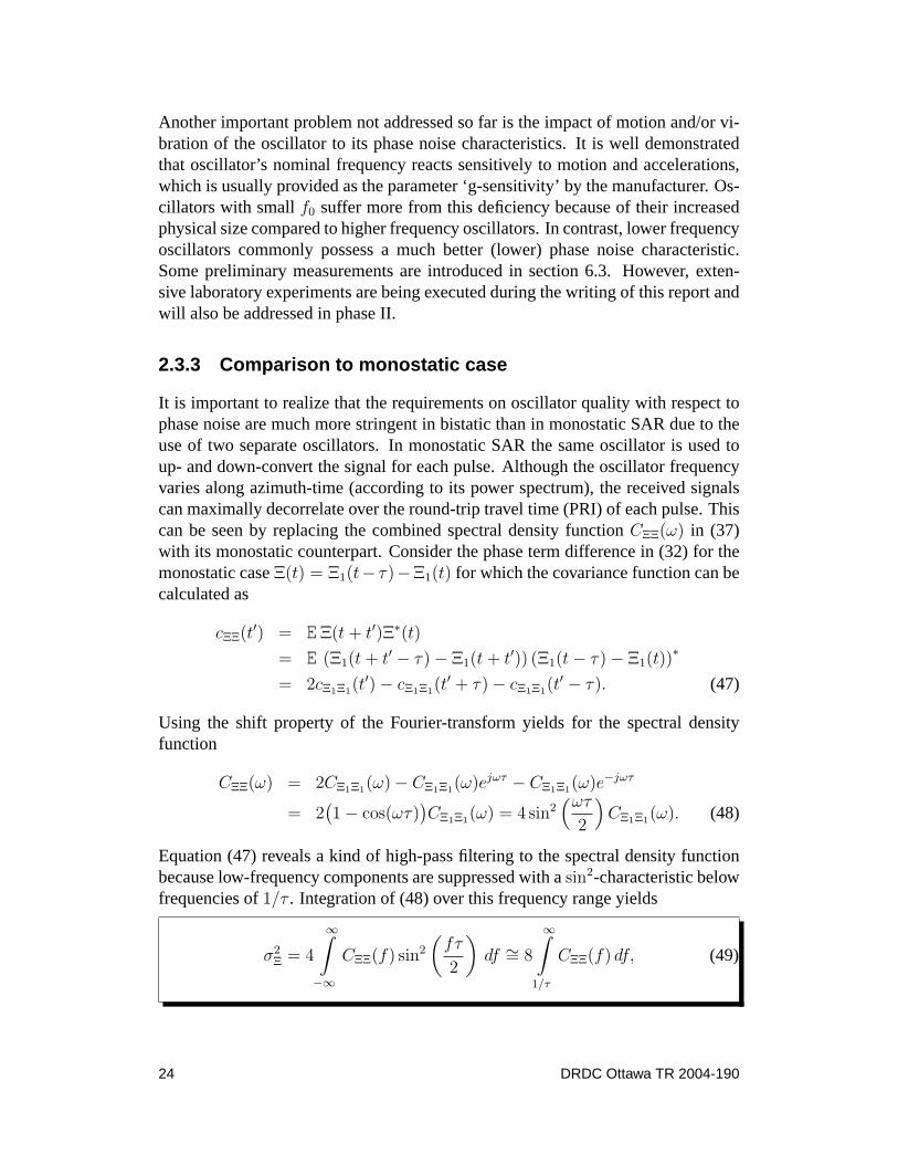
2.3.3 Comparison to monostatic case

It is important to realize that the requirements on oscillator quality with respect tophase noise are much more stringent in bistatic than in monostatic SAR due to theuse of two separate oscillators. In monostatic SAR the same oscillator is used toup- and down-convert the signal for each pulse. Although the oscillator frequencyvaries along azimuth-time (according to its power spectrum), the received signalscan maximally decorrelate over the round-trip travel time (PRI) of each pulse. Thiscan be seen by replacing the combined spectral density functionCΞΞ(ω) in (37)with its monostatic counterpart. Consider the phase term difference in (32) for themonostatic caseΞ(t) = Ξ1(t− τ)−Ξ1(t) for which the covariance function can becalculated as

cΞΞ(t′) = EΞ(t + t′)Ξ∗(t)

= E (Ξ1(t + t′ − τ)− Ξ1(t + t′)) (Ξ1(t− τ)− Ξ1(t))∗

= 2cΞ1Ξ1(t′)− cΞ1Ξ1(t

′ + τ)− cΞ1Ξ1(t′ − τ). (47)

Using the shift property of the Fourier-transform yields for the spectral densityfunction

CΞΞ(ω) = 2CΞ1Ξ1(ω)− CΞ1Ξ1(ω)ejωτ − CΞ1Ξ1(ω)e−jωτ

= 2(1− cos(ωτ)

)CΞ1Ξ1(ω) = 4 sin2

(ωτ

2

)CΞ1Ξ1(ω). (48)

Equation (47) reveals a kind of high-pass filtering to the spectral density functionbecause low-frequency components are suppressed with asin2-characteristic belowfrequencies of1/τ . Integration of (48) over this frequency range yields

σ2Ξ = 4

∞∫−∞

CΞΞ(f) sin2

(fτ

2

)df ∼= 8

∞∫1/τ

CΞΞ(f) df, (49)


which corresponds to an monostatic IISLR of−28 dB for the Symmetricom,−40dB for the low noise oscillator from Wenzel, and about−52 dB for the ultra-lowphase noise oscillator form OSC.


3 Bistatic observation time

One parameter of major importance for bistatic SAR is the time period for which ascatterer on a particular location on the ground is observed simultaneously by bothradars. In order to calculate this time, the individual time-dependent range vec-tors (1) for the transmitter and receiver are transformed into the antenna coordinatesystem by

Ri,a(t, r) = Las Ri,s(t, r) = L(Φi(t), 0, Ψi(t))L(π, 0, Ψv) Ri,s(t, r) (50)

for i = 1, 2, whereΨv denotes the constant course angle defined in appendix E.3.Φi(t) andΨ(t) are the azimuth and elevation (depression) angles (appendix E.4)which are in general adjusted over time, depending on the particular SAR modeused:

• Stripmap or squinted stripmap mode:Φi(t) = Φi,0 andΨi(t) = Ψi,0, whereΦi,0 andΨi,0 are the squint angle and depression angle to the center of the sceneat timet = 0.

• Spotmode:Φi(t) andΨi(t) are updated from pulse to pulse so that the antennais always pointing at center of the scene (r = 0).

It is obvious that the bistatic observation time can almost be arbitrarily chosen inspotmode operations, as long as the scatterer is within the overlap region of both an-tenna footprints. For stripmap operations, however, where the beam pointing of theantenna is kept fixed over the measurement interval, the bistatic observation time isprincipally limited. Depending on the flight trajectories of both platforms, the max-imum observation time may vary significantly for different areas on the ground. Inorder to assess whether a particular point on the ground is simultaneously ‘seen’ ata certain instant in time, the directional cosineui and sinevi of both radars must becomputed:

ui(t, r) =u′xRi,a(t, r)

||Ri,a(t, r)||= sin Ψi(t, r) cos Φi(t, r)

vi(t, r) =u′zRi,a(t, r)

||Ri,a(t, r)||= sin Φi(t, r), (51)

whereux = [1, 0, 0]′ anduz = [0, 0, 1]′. The bistatic observation timeTb is thengiven as the integral

Tb(r) =

∞∫−∞

I1(t, r) · I2(t, r) dt, (52)


where the indicator functions are defined as

Ii(t, r) =

1 if |ui(t, r)− u0,i| ≤ u3dB,i/2

|vi(t, r)− v0,i| ≤ v3dB,i/20 elsewhere.

(53)

u0,i andv0,i are the directional cosine and sine corresponding to the azimuth and el-evation anglesΦ0,i andΨ0,i of both platforms to the scene center at time origin. Theantenna beamwidth in either direction are herein denoted by the subscript ‘3dB’.

By inserting (1) into (51), it is possible to solve the inequality of (53) analytically.The derivation is exemplified below for the directional cosine where, for conve-nience, the transmitter/receiver subscripti is omitted:

u(t, r) =u′xLas(R0 − r) + u′xLasv t√

||R0 − r||2 + 2(R0 − r)′v t + ||v||2 t2≤ η, (54)

whereη = u0 + u3dB/2, which can be re-written as

(a0 + a1 t)2 ≤ η2(b0 + b1 t + b2 t2

)c2 t2 + c1 t + c0 = 0, (55)

with

a0 = u′xLas(R0 − r)

a1 = u′xLasv

b0 = ||R0 − r||2

b1 = 2(R0 − r)′v

b2 = ||v||2, (56)

andc0 = a20 − η2b0, c1 = 2a0a1 − η2b1 andc2 = a2

1 − η2b2. The solution of (55) isgiven as

t1,2 ≤ − c1

2c2

∓

√−c0

c2

+c21

4c22

for c2 6= 0, (57)

Depending on the sign ofc2, different cases for the solution must be distinguished.According to Fig. 10, there is either no real solution if the parabola does not crossthex-axis, or two real solutions in the specified gray regions.


t1

t2

t1

t2

No real solution

No real solution

Figure 10 : Regions of possible solutions for the bistatic observation time.

Comparing the minima and maxima of the individual solutions foru andv for bothtransmitter and receiver yields the maximum observation time for each scatterer onthe ground:

Tb(r) = max (0, tmax(r)− tmin(r)) , (58)

where

tmin = max (tu11 , tu2

1 , tv11 , tv2

1 )

tmax = min (tu12 , tu2

2 , tv12 , tv2

2 ) , (59)

and where ‘max(x, y, z)’ means the largest of each valuex, y andz.

Figure 11 demonstrates the variation of bistatic observation timeTb(r) given by(58) for each pixel on the ground for different bistatic angles between transmitterand receiver. In this case, the transmitter is chosen to be an aircraft with parameterslisted in Table 4. The receiver is located on top of a stationary tower with parame-

Table 4: Airborne transmitter parameters.

Altitude H1 = 5000 mVelocity v1 = 132 ux m/s

Elevation angle to scenecentre att = 0 Φ0,1 = 10◦

Squint angle to scenecentre att = 0 Ψ0,1 = 0◦

Antenna pattern sincAzimuth beamwidth u3dB,1 = 4◦

Elevation beamwidth u3dB,1 = 2.5◦

ters listed in Table 5, where the receiver squint (azimuth) angleΨ0,2 is varied, seeappendix F.Ψ0,2 = 0◦ means the aircraft is flying behind the tower and both an-tennas are pointing in the same direction (i.e., a quasi-monostatic geometry). Incontrast,Ψ0,2 = 0◦ indicates that the aircraft is flying in front of the radar perpen-dicular to the receiver antenna pointing direction, resulting in a forward-scattering


Table 5: Tower receiver parameters.

Altitude H2 = 20 mVelocity v2 = 0 m/s

Elevation angle to scenecentre att = 0 Φ0,2 = 0.5◦

Antenna pattern sincAzimuth beamwidth u3dB,2 = 45◦

Elevation beamwidth u3dB,2 = 10◦

geometry. It is evident that the maximum observation time is relatively large (Ts ≈12 to 16 s) because of the shallow elevation angle of the transmitter, which resultsin large distances to the scene on the ground. A larger distance means an increasedsynthetic aperture time for a given azimuth beamwidth. Also recognizable are thedifferent regions on the ground which are bistatically observable due to the changein receiver location and orientation. Of course, much more complex illuminationshapes are usually possible when the receiver is also moving.


0

2

4

6

8

10

12

14

16

x−axis [m]

y−ax

is [m

]

−4000 −3000 −2000 −1000 0 1000 2000 3000 4000

−4000

−3000

−2000

−1000

0

1000

2000

3000

4000

(a) Quasi-monostatic geometry, bistatic an-gle = 0◦.

0

2

4

6

8

10

12

14

16

x−axis [m]

y−ax

is [m

]

−4000 −3000 −2000 −1000 0 1000 2000 3000 4000

−4000

−3000

−2000

−1000

0

1000

2000

3000

4000

(b) Bistatic angle =45◦.

0

2

4

6

8

10

12

14

16

x−axis [m]

y−ax

is [m

]

−4000 −3000 −2000 −1000 0 1000 2000 3000 4000

−4000

−3000

−2000

−1000

0

1000

2000

3000

4000

(c) Bistatic angle =90◦.

0

2

4

6

8

10

12

14

16

x−axis [m]

y−ax

is [m

]

−4000 −3000 −2000 −1000 0 1000 2000 3000 4000

−4000

−3000

−2000

−1000

0

1000

2000

3000

4000

(d) Bistatic angle =135◦.

0

2

4

6

8

10

12

14

16

x−axis [m]

y−ax

is [m

]

−4000 −3000 −2000 −1000 0 1000 2000 3000 4000

−4000

−3000

−2000

−1000

0

1000

2000

3000

4000

(e) Bistatic angle =150◦.

0

2

4

6

8

10

12

14

16

x−axis [m]

y−ax

is [m

]

−4000 −3000 −2000 −1000 0 1000 2000 3000 4000

−4000

−3000

−2000

−1000

0

1000

2000

3000

4000

(f) Forward-looking geometry, bistatic angle= 180◦.

Figure 11: Bistatic observation time of ground range scatterer. Stationary re-ceiver and airborne transmitter for varying bistatic angles Ψ0,2.


4 Bistatic SAR performance analysis

The aim of this section is to derive tractable mathematical tools to determine thebistatic SAR resolution for individual points on the ground for arbitrary transmitterand receiver flight geometries. The term resolution in this context means the abilityto separate close targets in different areas on the ground. A similar approach wasapplied for a parasitic SAR system in [15].

These tools will allow performance comparisons of different flight geometries with-out the necessity of SAR processing, i.e., the complex and sometimes time-consumingcomputation of the point spread function, e.g., [17]. They could also be used in anopposite way during the flight planning phase of operations to determine the neces-sary flight geometry (and velocities) for a required minimum ground resolution ina particular region of interest.

It is important to note that the analysis herein is based on a fully three-dimensionalscenario, i.e., it is not restricted to two-dimensional geometries as is sometimesdone in the literature. Further, constant velocities for the radar platforms are onlychosen for clarity of the derivation. Accelerations or non-constant altitudes caneasily be included in the analysis.

4.1 Preliminaries: Doppler-bandwidth,Doppler-gradient and the k-space

In order to determine SAR resolution, it is crucial to understand the physical phe-nomena describing the composition of the synthetic aperture and therewith allow-ing the imaging of the desired reflectivity with high resolution. This is even moreimportant as the general bistatic case is usually much more complex than the rela-tively simple monostatic case. For the monostatic case, for instance, it is commonin the literature to use the Doppler-bandwidth (the maximum spread of Dopplerfrequency) of a scatterer on the ground to calculate the corresponding azimuth(cross-range or Doppler) resolution. In this subsection we want to show that theidea of bandwidth can only be applied to the monostatic non-squinted case. In-stead of Doppler-bandwidth, the shape of the point spread function (and therewiththe resolution) is determined instead by the magnitude of the Doppler-gradient vec-tor, or, in even more general terms, by the the form and extent of the wavenumbervector or k-space. In fact, both are identical only for the very special case of side-looking monostatic SAR. An excellent introduction to this topic can be found inthe overview article by Ender [33]. Although the term ‘Doppler resolution’ mightbe somewhat misleading, because it is commonly linked to Doppler bandwidth, wehave adopted the term for notational convenience.


The starting point to determine the resolution of bistatic SAR is the three-dimensionalgeometry depicted in Fig. 3. The effective range vector from the transmitter (fromhereon indicated by subscript 1) to the pointr on the ground and back to the receiver(subscript 2) at timet is given as the sum

R(t, r) = R1(t, r) + R2(t, r) =(R0,1 − r

)+ v1t +

(R0,2 − r

)+ v2t, (60)

whereR0,i = Ri(0, 0) are the ranges from the scene center to either platform attime zero. Determined by the distance between the transmitter and the receiver, theresulting phase history of the received signal yields

φ(t, r) = k (||R1(t, r)||+ ||R2(t, r)||) , (61)

wherek = 2π/λ denotes the wavenumber. The Doppler frequency is given by thefirst derivative of (61) as

ωD(t, r) ≡ φ(t, r) =dφ(t, r)

dt=

kv′1((R0,1 − r) + v1t

)√((R0,1 − r) + v1t

)′ ((R0,1 − r) + v1t

)+k

v′2((R0,2 − r) + v2t

)√((R0,2 − r) + v2t

)′ ((R0,2 − r) + v2t

)= k

(v′1uR1

(t, r) + v′2uR2(t, r)

), (62)

whereua = a/||a|| is the unit vector in directiona. For simplicity, the unit vector indirectionRi will be referred to asui. Combining the scalark and the unit directionvectors to the wavenumber vectorki(t, r) = kui(t, r) with physical unit m−1, theDoppler frequency yields

ωD(t, r) = v′1 k1(t, r) + v′2 k2(t, r). (63)

Using (63), the slope of the Doppler frequency as the second derivative of the phasesD(t, r) ≡ φ(t, r) is given as

sD(t, r) =dωD(t, r)

dt= v′1 k1(t, r) + v′2 k2(t, r), (64)

which can be further written as

sD(t, r) = k (v′1u1(t, r) + v′2u2(t, r))


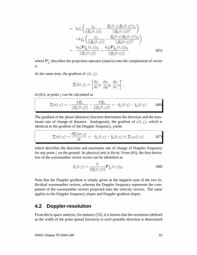
= kv′1

(v1

||R1(t, r)||− R1(t, r)R1(t, r)

′v1

||R1(t, r)||3

)+kv′2

(v2

||R2(t, r)||− R2(t, r)R2(t, r)

′v2

||R2(t, r)||3

)=

kv′1P⊥R1

(t, r)v1

||R1(t, r)||+

kv′2P⊥R2

(t, r)v2

||R2(t, r)||, (65)

whereP⊥a describes the projection operator (matrix) onto the complement of vector

a.

At the same time, the gradient ofφ(t, r):

∇φ(t, r) =

[∂φ

∂xx,

∂φ

∂yy,

∂φ

∂zz

]′,

in (61), at pointr can be calculated as

∇φ(t, r) = − kR1

||R1(t, r)||− kR2

||R2(t, r)||= −k1(t, r)− k2(t, r). (66)

The gradient of the phase (distance) function determines the direction and the max-imum rate of change of distance. Analogously, the gradient ofφ(t, r), which isidentical to the gradient of the Doppler frequency, yields

∇φ(t, r) =d∇φ(t, r)

dt= −k1(t, r)− k2(t, r) ≡ ∇ωD(t, r), (67)

which describes the direction and maximum rate of change of Doppler frequencyfor any pointr on the ground. Its physical unit is Hz/m. From (65), the first deriva-tive of the wavenumber vector vector can be identified as

ki(t, r) =k

‖Ri(t, r)‖P⊥

Ri(t, r)vi. (68)

Note that the Doppler gradient is simply given as the negative sum of the two in-dividual wavenumber vectors, whereas the Doppler frequency represents the com-ponent of the wavenumber vectors projected onto the velocity vectors. The sameapplies to the Doppler frequency slopes and Doppler gradient slopes.

4.2 Doppler-resolution

From this k-space analysis, for instance [33], it is known that the resolution (definedas the width of the point spread function) in each possible direction is determined


by the reciprocal of the maximum extent/spread of the k-set in this particular di-rection. The idea of using the gradient to calculate this maximum extent, i.e., toexamine the bistatic SAR resolution, was originally utilised in [34] and later alsoin [7, 35]. However, these authors only considered the wavenumber vectors at thetime origin and neglected their change over time, i.e., they assumed the gradient tobe constant over time. This is a rather crude approximation, which is valid only fornear-monostatic (non-squinted) configurations.

Including the time dependency of the Doppler gradient (67), the maximum k-setspread in Doppler direction, denoted bySD, can be calculated as the norm of thevector integral

SD(r) =1

2π

∥∥∥∥∥∥tmax∫

tmin

∇ωD(t, r) dt

∥∥∥∥∥∥ . (69)

The integral must be computed over the maximum bistatic observation time for theconsidered ground pointr. The timestmin andtmax denote the first and last instantin time that this ground point is ‘seen’ from both radar antennas, i.e., lies simulta-neously within both antenna patterns. For radar platforms traveling with constantvelocities, the bistatic observation time was calculated analytically in Section 3.

Using (67), this becomes in closed form

SD(r) =1

2π

∥∥∥∥∥∥tmax∫

tmin

k1(t, r) + k2(t, r) dt

∥∥∥∥∥∥=

1

λ‖u1(tmax, r)− u1(tmin, r) + u2(tmax, r)− u2(tmin, r)‖. (70)

Hence, the exact solution for the resolution in Doppler direction∆D in meter isgiven as the inverse of (70):

∆D(r) = S−1D =

λ

‖u1(tmax, r)− u1(tmin, r) + u2(tmax, r)− u2(tmin, r)‖. (71)

The physical interpretation of (71) is that the Doppler resolution is given as the in-verse of the sum of the maximum aspect angle variation of both platforms.

In contrast, the maximum Doppler bandwidthBD based on (63) is given as

BD(r) =k

‖v1‖2u′v1

(u1(tmax, r)−u1(tmin, r)

)+

k

‖v2‖2u′v2

(u2(tmax, r)−u2(tmin, r)

),

(72)which represents the sum of maximum aspect angle variation projected onto ei-ther flight direction. In the monostatic case, withu1(tmax, r) − u1(tmin, r) ≡


u2(tmax, r) − u2(tmin, r), which we will calla for convenience, the Doppler band-width is

BD(r) =k

π‖v‖u′va =

2‖v‖λ‖a‖u′vua. (73)

Equation (73) reveals the well-known Doppler bandwidth, for which the resolutionis calculated through∆′

D = ‖v‖/|BD|.

From (71) it is evident thatBD and SD are only identical ifu′vua = 1. Thesetwo vectors are only collinear for a special symmetric geometry, namely a strictlyside-looking SAR.

4.2.1 Special cases

To gain deeper insight into the ramifications of (71), it is helpful to look at somespecial cases of bistatic geometry.

4.2.1.1 Monostatic with omnidirectional antenna pattern

In the monostatic case when the two direction vectorsu1 andu2 are identical, i.e.,u = u1 = u2. An omnidirectional antenna diagram results in a theoretically unlim-ited observation time of the ground pointr, i.e.,tmin,max = ∓∞ with

limt→±∞

u(t, r) = limt→±∞

(R0,1 − r) + vt√‖R0,1 − r‖2 + 2v′(R0,1 − r)t + ‖v‖2 t2

= ± v

‖v‖= ±uv. (74)

As expected, the unit direction vector converges to the unit velocity vector for infi-nite time. Hence, inserting (74) in (71) leads to

∆D =λ

2‖u(∞, r)− u(−∞, r)‖=

λ

2‖2uv‖=

λ

4, (75)

the well known maximal Doppler resolution of a quarter-wavelength, independentof the scatterer location.

4.2.1.2 Monostatic stripmap with realistic antenna pattern

The maximum observation time for a monostatic geometry is given as the periodof time between entering and leaving the mainbeam during the overflight. Thesetimes are

tmin,max = ∓θ3dB

2

‖R0 − r‖‖v‖

, (76)


which in turn yields

u(tmax, r)− u(tmin, r) =θ3dB

2

v

‖v‖(77) 1√

1 +(R0−r)′v‖v‖ ‖R0−r‖θ3dB +

θ23dB

4

+1√

1 +(R0−r)′v‖v‖ ‖R0−r‖θ3dB −

θ23dB

4

.

For a non-squinted (or slightly squinted) geometry withuR0−r ⊥ v, the differencein (77) can be approximated asu(tmax, r)− u(tmin, r) ≈ θ3dBv/‖v‖, which resultsin the well known range-independent (azimuth) resolution

∆D =λ

‖2uv θ3dB‖=

A

2, (78)

whereA = λ/θ3dB denotes the real aperture of the monostatic antenna.

4.2.1.3 Bistatic with omnidirectional antenna pattern

Analogous to (74), the individual direction vectors areui(∞, r) − ui(−∞, r) =2uvi

, which inserted into (71) leads to

∆D =λ

2‖uv1+ uv2

‖=

λ

4√

1 + cos α, (79)

whereα denotes the angle between the two velocity vectors. It is apparent thatthe bistatic Doppler resolution is always lower than that of the monostatic case,except when the two platform fly exactly parallel. In contrast, the resolution goesto infinity when the two platforms fly anti-parallel, i.e.,cos α = −1, because theaspect angle variation/spread for each platform cancels out exactly.

4.2.1.4 Bistatic stripmap with realistic antenna pattern

Let us assume that the maximum bistatic observation time is exclusively determinedby one of the platforms, e.g., by the transmitter:

tmin,max ≡ tmin,1,max,1 = ∓θ1

2

‖R0,1 − r‖‖v1‖

, (80)

where for simplicity of notation the subscript ‘3dB’ for the transmitter beamwidthhas been omitted. This assumption is not restrictive. In contrast, it would alwaysbe fulfilled in cases of high-flying (maybe orbiting) illuminators and relatively lowflying receivers with‖R0,1−r‖ � ‖R0,2−r‖. In order to keep the PRF reasonablysmall, i.e., to avoid range ambiguities while maintaining a sufficient swathwidth,


high altitude SARs need to be equipped with rather large antennas, which meansθ1 � θ2. Analogous to (77), the direction vector difference for the transmitter isgiven as

u1(tmax,1, r)− u1(tmin,1, r) ≈ θ1v1

‖v1‖, (81)

whereas that of the receiver is

u2(tmax,1, r)− u2(tmin,1, r) = (82)

θ1

2

‖R0,1 − r‖‖v1‖

v2

2√1 +

‖R0,1−r‖2 ‖v2‖2‖R0,2−r‖2 ‖v1‖2

θ21

4

≈ θ1

‖R0,1 − r‖‖v1‖

v2,

where it has been assumed that both radars work in quasi-stripmap mode withR′

0,ivi � 1. Inserting (81) and (82) into (70) yields

BD =θ1

λ‖v1‖

√‖R0,1 − r‖2

‖R0,2 − r‖2‖v2‖2 + 2

‖R0,1 − r‖‖R0,2 − r‖

v′1v2 + ‖v1‖2. (83)

For two special flight geometries this term can be further simplified. If the two plat-forms fly exactly perpendicular to each other, i.e.,v′1v2 = 0, the Doppler resolutionas the inverse of (83) becomes

∆⊥D = A1

(√1 +

‖R0,1 − r‖2 ‖v2‖2

‖R0,2 − r‖2 ‖v1‖2

)−1

, (84)

and in case they both fly parallel or anti-parallel, i.e.,v′1v2 = ±‖v1‖ ‖v2‖ it be-comes

∆‖D = sign

(1±

‖R0,1 − r‖ ‖v2‖‖R0,2 − r‖ ‖v1‖

)A1

1± ‖R0,1−r‖ ‖v2‖‖R0,2−r‖ ‖v1‖

, (85)

whereA1 = λ/θ1 denotes the real aperture of the transmitter. In (85) it is interestingto note that the Doppler resolution will be better than that of a monostatic SAR onthe transmitter platform when the ratio between distances and the speeds of the twoplatforms are chosen appropriately, e.g.,‖R0,1− r‖/‖v1‖ > ‖R0,2− r‖/‖v2‖. Thephysical reason behind this is that the combined aspect angle variation/spread ofhigh flying illuminator and low-flying receiver can be larger compared to that ofa high-flying monostatic system. In [36], this result was derived on a multi-pageanalysis via the width of the actual point spread function.

Fig. 12 shows the expected bistatic observation time and the corresponding Dopplerresolution for the bistatic airborne scenario listed in Table 6. One can recognizethat the bistatic observation time is non-symmetrically distributed along the ‘bistat-ically illuminated’ area. It is clear that the Doppler resolution will be worse forareas where the observation time is small, such at the edges.


Table 6: Bistatic airborne-airborne configuration

Parameter Transmitter Receiver

Altitude H1 = 7000 m H2 = 15, 000 mVelocity v1 = 130 ux m/s v2 = 220 m/s

Course angle Ψps,1 = 0◦ Ψps,2 = 45◦

Elevation angle to scenecentre att = 0 Φ0,1 = 45◦ Φ0,2 = 35◦

Squint angles to scenecentre att = 0 Ψ0,1 = 0◦ Ψ0,2 = 90◦

Antenna pattern sinc sincAzimuth beamwidth u3dB,1 = 3◦ u3dB,2 = 3◦

Elevation beamwidth v3dB,1 = 20◦ v3dB,2 = 20◦

Wavelength λ = 0.0565 mPulse bandwidth B = 50 MHz

Sampling frequency fs = 50 MHzPulse Length T = 5µs

PRF 680 Hz

4.2.1.5 Bistatic stripmap with realistic antenna pattern and stationaryreceiver

From equations (83) to (85), it is evident that the Doppler resolution for a stationaryreceiver withv2 = 0 is identical to the real aperture of the transmitter, independentof the location on the ground:

∆ZD = A1, (86)

whereZ symbolises the moving transmitter and the stationary receiver. This valueis exactly one-half of the maximum value for a conventional monostatic stripmapSAR. Of course, the bistatic Doppler resolution can always be enhanced by pointingthe antenna beam on the same spot on the ground (spotmode) during the flight, andthereby increasing the bistatic observation time, and in turn, the extent of the k-space. In contrast, increasing the beamwidth of the stationary receiver antennawill not enhance the Doppler resolution because the k-space spread is exclusivelydetermined by the moving transmitter. However, a larger receiver beamwidth willincrease the imageable area on the ground.

The resolution for the airborne-tower scenario introduced in Tables 4 and 5 is deter-mined by the transmitter azimuthal beamwidth∆Z

D = λ/u3dB,1 = 0.4516 m. Sincethe Doppler resolution for a stationary receiver is constant inside the bistaticallyilluminated region, it is not explicitly plotted.

It is important to note that the Doppler gradient (67) is only varying slightly over


x−axis [m]

y−ax

is [m

]

−3000 −2000 −1000 0 1000 2000 3000

−3000

−2000

−1000

0

1000

2000

3000 0

0.5

1

1.5

2

2.5

3

3.5

4

4.5

(a) Bistatic observation time in seconds.

−3000 −2000 −1000 0 1000 2000 3000

−3000

−2000

−1000

0

1000

2000

3000 0

0.5

1

1.5

2

2.5

3

3.5

4

4.5

5

(b) Doppler resolution in meters.

Figure 12: Bistatic observation time and ground Doppler resolution for the air-borne transmitter and airborne receiver configuration listed in Table 6.

time in many practical cases, such as side-looking or slightly squinted SAR modes.In such cases,k can be treated as constant over time and can be taken out of theintegral in (70), i.e.,

BD ≈Tb

λ‖u1(0, r) + u2(0, r)‖ , (87)

whereTb = tmax− tmin is the bistatic observation time. Replacingui(0, r) with thethe projections (68) at the time origin yields

BD ≈Tb

λ

∥∥∥∥ 1

‖R0,1 − r‖P⊥

R1(0, r)v1 +

1

‖R0,2 − r‖P⊥

R2(0, r)v2

∥∥∥∥=

Tb

λ

∥∥∥∥(I− u1(0, r)u′1(0, r)) v1

‖R0,1 − r‖+

(I− u2(0, r)u′2(0, r)) v2

‖R0,2 − r‖

∥∥∥∥ , (88)

which is identical to the result originally introduced by Cardillo [34], and later in[37]. For only slightly squinted geometries whereu′i(0, r)uvi

≈ 0, it is easy toshow that identical results as those for the previous special cases (shown above)can be achieved. However, (71) represents the exact solution for any SAR modeand geometry, and should, therefore, be preferred.

4.2.2 Ground plane

In most cases one is interested in the resolution on the ground plane, i.e., on theseparability of two closely located points on Earth’s surface. In order to accommo-date this, the generally three-dimensional Doppler gradient vector can, for instance,be projected onto the flat ground plane. In other words, the maximum change of


Doppler on the ground is along the projection of the gradient onto the ground. Ap-plying the constant projection matrix

P⊥zs

= (I− zsz′s) =

1 0 00 1 00 0 0

(89)

to the Doppler gradient in (67)

∇(g)ωD(t, r) = P⊥zs∇ωD(t, r) (90)

and following the analysis form (69) to (71), yields the ground resolution of

∆(g)D (r) =

λ∥∥∥P⊥zs

(u1(tmax, r)− u1(tmin, r) + u2(tmax, r)− u2(tmin, r)

)∥∥∥ . (91)

4.3 Range-resolution

The idea of using the gradient to determine the bistatic resolution can also be ap-plied in the fast-time direction. Although there is no perspicuous range direction inbistatic geometry, it is convenient to keep using this term. According to (1) and (3),the total travel timeτ of the transmitted pulse to a scatterer on the ground (locatedat r) and further to the receiver is given by

τ(t, r) =1

c

(‖R1(t, r)‖+ ‖R2(t, r)‖

), (92)

wherec denotes the speed of light. The gradient

∇τ(t, r) =1

c

(u1(t, r) + u2(t, r)

)(93)

represents the direction and size of the maximum change of travel time. Althoughthe travel time is strictly speaking dependent on time (varying position of the radars),the change of the gradient over the entire aperture time is typically small, so that itcan be neglected in all practical cases. Hence, it is sufficient to analyse the gradientonly at the time origin, i.e., we define two nearby points to be resolved in rangeas long as they are separable att = 0. For a monostatic system, for instance, thismeans that echoes of two closely spaced scatterers are located in different rangecells along the entire synthetic aperture in the raw data matrix.

Since the receiver measures different arrival times proportional to the system band-width B, i.e., in a raster of spacingδt = 1/B, the range resolution can be writtenas

∆R(r) =1/B

‖∇τ(0, r)‖=

c

B ‖u1(0, r) + u2(0, r)‖, (94)


whereui(0, r) ≡ u0,i = (R0,i − r)/‖R0,i − r‖.

Equating the two directional unit vectors in (94) confirms the well known constantslant-range resolution of∆R(r) = c/(2B) for a monostatic scenario. In the bistaticcase (94) can be re-written as

∆R(r) =c√2B

1√1 + cos α(r)

(95)

whereα(r) denotes the angle between the range vectors from the pointr on theground to the receiver and transmitter, respectively.

4.3.1 Ground plane

Analogously to (90), the gradient vector (93) must be projected onto the two-dimensional ground plane in order to evaluate the ground range resolution on theflat Earth’s surface. Therefore, applying the projection (89) to the gradient vectoryields the general form of the bistatic range resolution

∆(g)R (r) =

1/B

‖∇(g)τ(0, r)‖=

1/B

‖P⊥zs∇τ(0, r)‖

=c/B

‖P⊥zs

u0,1(r) + P⊥zs

u0,2(r)‖. (96)

Figure 13 shows the ground range resolution over varying bistatic angles for the air-borne transmitter and tower receiver geometry used previously, see Tables 4 and 5.The loss in range resolution for less favourable geometries becomes evident, espe-cially for the area around the line connecting the receiver and the transmitter. Here,the resolution decreases drastically from roughly 30 cm to 40 m. However, reason-able imaging (in the meter-range resolution) should be possible for pixels furtheraway from this line, even for a forward-scattering geometry .

4.3.2 Equivalent bistatic nadir hole

From (96), it is evident that the ‘bistatic nadir hole’ is given at the location onthe groundr at which the norm of the travel-time gradient vanishes. Around thislocation, the ground range resolution tends to infinity, i.e., meaningful imaging isimpossible. Re-writing the projection matric in (89) asP⊥

zs= xsx

′s + y

sy′

s, we get

∇τ (g)(r) =1

c

(x′su0,1(r) + x′su0,2(r)

)xs +

1

c

(y′

su0,1(r) + y′

su0,2(r)

)y

s. (97)

In order for the norm of (97) to be zero, both components must satisfy

x′s

(u0,1(r0) + u0,2(r0)

)= 0

y′s

(u0,1(r0) + u0,2(r0)

)= 0, (98)


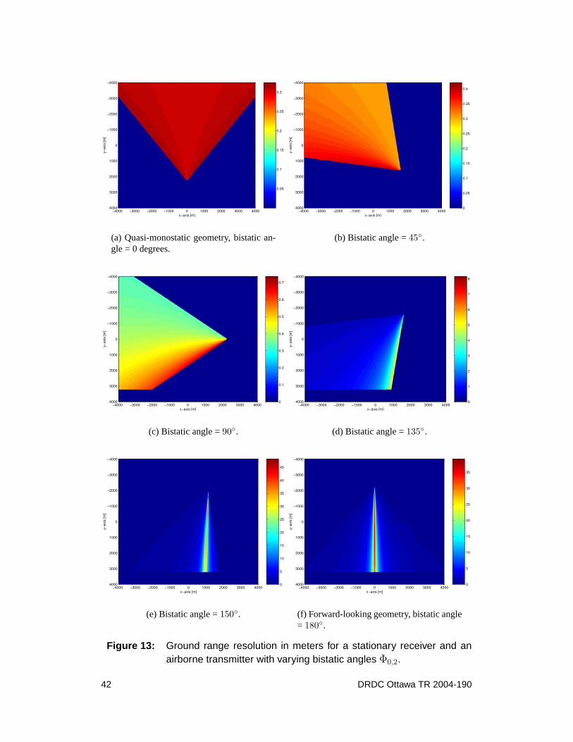
0.05

0.1

0.15

0.2

0.25

0.3

x−axis [m]

y−ax

is [m

]

−4000 −3000 −2000 −1000 0 1000 2000 3000 4000

−4000

−3000

−2000

−1000

0

1000

2000

3000

4000

(a) Quasi-monostatic geometry, bistatic an-gle = 0 degrees.

0

0.05

0.1

0.15

0.2

0.25

0.3

0.35

0.4

x−axis [m]

y−ax

is [m

]

−4000 −3000 −2000 −1000 0 1000 2000 3000 4000

−4000

−3000

−2000

−1000

0

1000

2000

3000

4000

(b) Bistatic angle =45◦.

0

0.1

0.2

0.3

0.4

0.5

0.6

0.7

x−axis [m]

y−ax

is [m

]

−4000 −3000 −2000 −1000 0 1000 2000 3000 4000

−4000

−3000

−2000

−1000

0

1000

2000

3000

4000

(c) Bistatic angle =90◦.

0

1

2

3

4

5

6

7

8

x−axis [m]

y−ax

is [m

]

−4000 −3000 −2000 −1000 0 1000 2000 3000 4000

−4000

−3000

−2000

−1000

0

1000

2000

3000

4000

(d) Bistatic angle =135◦.

0

5

10

15

20

25

30

35

40

45

x−axis [m]

y−ax

is [m

]

−4000 −3000 −2000 −1000 0 1000 2000 3000 4000

−4000

−3000

−2000

−1000

0

1000

2000

3000

4000

(e) Bistatic angle =150◦.

0

5

10

15

20

25

30

35

x−axis [m]

y−ax

is [m

]

−4000 −3000 −2000 −1000 0 1000 2000 3000 4000

−4000

−3000

−2000

−1000

0

1000

2000

3000

4000

(f) Forward-looking geometry, bistatic angle= 180◦.

Figure 13: Ground range resolution in meters for a stationary receiver and anairborne transmitter with varying bistatic angles Φ0,2.


i.e., must simultaneously vanish atr0. In other words, the vector given as the sumof the two unit vectors pointing from the locationr0 to either radar must be perpen-dicular to the ground plane, i.e.,u0,1(r0) + u0,2(r0) ⊥ xs, ys

.

In monostatic SAR, whereu0,1(r) = u0,2(r), this is true forr0 directly beneaththe radar platform, which is typically not illuminated by the antenna pattern. Inbistatic SAR, however, the equivalent nadir may shift into the viewable/imagedarea depending on the bistatic geometry, e.g.,‖R0,1 � R0,2‖, as shown in Fig. 14.

H1

u0,1

u0,2

xs

zs

ys

r0

H2

Figure 14 : Illustration of the equivalent bistatic nadir hole at r = r0.


5 Bistatic SAR raw data simulation

To develop and test techniques and algorithms to process bistatic SAR data, it is es-sential to investigate and compare their fidelity and quality on simulated data, i.e.,raw data sets obtained under ideal conditions. The developed and implementedpoint target simulator comprises all necessary components to be realistic: 3D-platform geometry and motion vectors, point target location and reflectivity, imag-ing geometry (such as distances between illuminator-target-receiver and coordinatetransformations) as well as antenna pattern and variable pointing.

In a first step, an airborne bistatic SAR simulator with constant velocities and al-titudes and a flat Earth assumption has been developed and coded in MATLAB.The simulated SAR configurations comprise the simple stripmap mode as well asmore sophisticated modes where the antenna is continuously steered onto the scenecenter during the flight (spotmode, sliding stripmode, etc.). All required coordinatesystems and angular transformations are defined in appendices D and E. The userinputs are the basic radar system parameters: wavelengthλ, pulse bandwidthB,sampling frequencyfs, pulse LengthT , and the pulse repetition frequency PRF, aswell as the transmitter and receiver parameters at the time origin listed in Tables 4and 5.

In order to determine the maximum raw data field size in the Doppler direction,the maximum observation timeTb,max is calculated via (59) for each pixel withina pre-specified area on the ground. The maximum field size in the range directionis determined by the longest and shortest distance to any pixel. Half a chirp-lengthBT/2 is added on either side of the raw data field to prevent focussing errors atthe edges of the specified regions. The pre-specified region on the ground can nowbe sparsely filled withP scatterer points, where each point is characterised by itsxs, ys-location and its backscatter amplitude (radar cross section (RCS)). As refer-ence, the bistatic distance to the center of the scene at the time origin is calculatedas‖R0‖ = ‖R0,1‖+ ‖R0,2‖.

The actual raw data generation is now executed in a straightforward fashion, namely,via the superposition of each point target echo at each pulse transmission time (po-sition). Instead of summing the reflected echoes in the time domain, it is com-putationally more efficiently performed in the Fourier-domain. Here the time de-lay, which requires interpolation, corresponds to a multiplication with a linear fre-quency ramp. To achieve this, the ideal transmit pulse in baseband, (2),

s(ns) = exp

(jπ

B

T

(ns

fs

)2)

for ns = −Ns/2, . . . , Ns/2, (99)

andNs = fix(BT ) is transformed into the frequency domainS(ms) = F(s(ns)

).


For each pulse indexnp the range vectorsRi(np/PRF, r) from either platform tothe particular scatterer are computed via (1). Transforming these vectors into the an-tenna coordinate system with (E.8), i.e., by application ofLap(Φ0,i, Ψ0,i)Lps(Ψp,i)and using equations F.3, yields the required aspect and elevation angles to this scat-terer. These angles are then used to calculate the antenna pattern weighting. Thedelay timeτ(np, r) from transmitter to the scatterer located atr and to the receiveris given as

τ(np, r) =‖R1(np/PRF, r)‖+ ‖R2(np/PRF, r)‖ − ‖R0‖

c(100)

wherec denotes the speed of light. The phase multiplication

S(ms) · exp(− j2πf(ms)τ(np)

), (101)

wheref(ms) denotes a frequency bin in the RF domain, includes on one hand therange cell migration for longer synthetic aperture times, and on the other hand, alsoapplies the Doppler induced phase history. Weighting with the antenna pattern,adding up the returns from all scatterers and applying the inverse Fourier-transformto the result, leads to the desired raw data signal for the particular pulse index. Thisprocedure must be repeated for all pulses.

Figure 15 (a) shows the real part of simulated bistatic SAR raw data for a stationaryreceiver scenario. In order to keep the raw data field size reasonably small, a C-bandtransmitter was chosen; the system parameters in Table 7 are similar to those of theEnvironment Canada Convair-580 aircraft [38]. Since the illumination pattern isnot symmetric on the ground for this perpendicular configuration, see Fig. 11, theslow time origin does not occur at the center of the x-axis. In the real part ofthe raw data, typical Fresnel-rings are visible representing ‘height contours’ of thetwo-dimensional chirp function. Further, the ‘sinc’-antenna pattern weighting inthe Doppler direction can be recognized in the the magnitude plot, Fig. 15 (b), aswell as the range migration of the echo-pulse through various range cells.

Currently, a spaceborne version of a bistatic SAR simulator is under development.It is based on a fixed, Earth-centered, coordinate system and, in its final extensionwill use an orbit propagator software module to determine the satellite’s state vec-tors at each pulse transmission time. The scatterers are placed onto the curved Earthsurface and the Earth’s rotation will be taken into account.


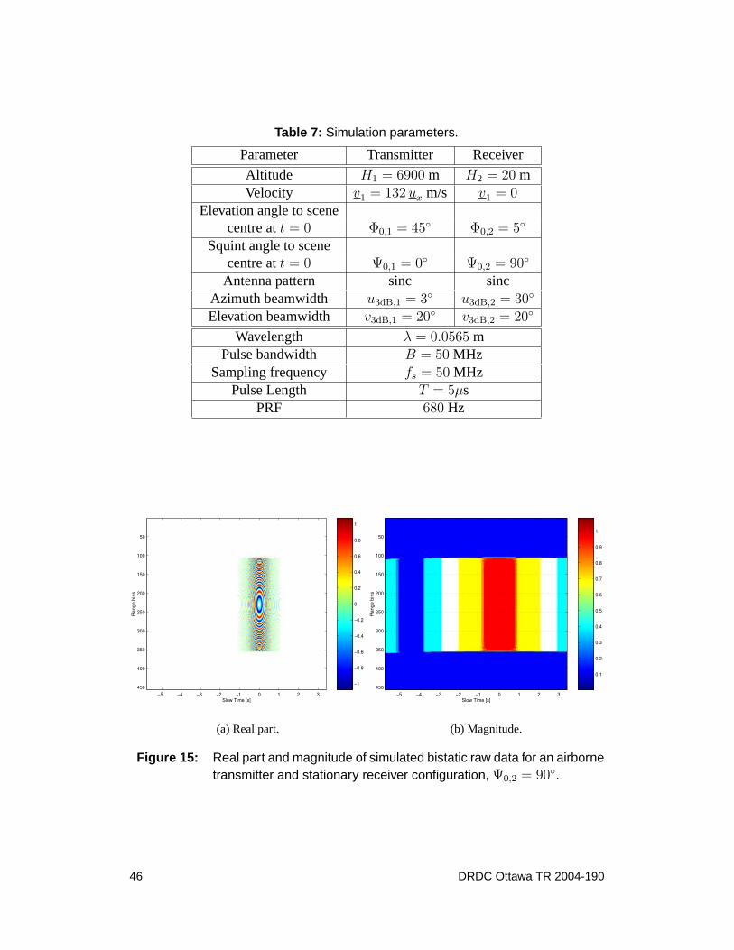
Table 7: Simulation parameters.

Parameter Transmitter Receiver

Altitude H1 = 6900 m H2 = 20 mVelocity v1 = 132 ux m/s v1 = 0

Elevation angle to scenecentre att = 0 Φ0,1 = 45◦ Φ0,2 = 5◦

Squint angle to scenecentre att = 0 Ψ0,1 = 0◦ Ψ0,2 = 90◦

Antenna pattern sinc sincAzimuth beamwidth u3dB,1 = 3◦ u3dB,2 = 30◦

Elevation beamwidth v3dB,1 = 20◦ v3dB,2 = 20◦

Wavelength λ = 0.0565 mPulse bandwidth B = 50 MHz

Sampling frequency fs = 50 MHzPulse Length T = 5µs

PRF 680 Hz

−1

−0.8

−0.6

−0.4

−0.2

0

0.2

0.4

0.6

0.8

1

Slow Time [s]

Ran

ge b

ins

−5 −4 −3 −2 −1 0 1 2 3

50

100

150

200

250

300

350

400

450

(a) Real part.

0.1

0.2

0.3

0.4

0.5

0.6

0.7

0.8

0.9

1

Slow Time [s]

Ran

ge b

ins

−5 −4 −3 −2 −1 0 1 2 3

50

100

150

200

250

300

350

400

450

(b) Magnitude.

Figure 15: Real part and magnitude of simulated bistatic raw data for an airbornetransmitter and stationary receiver configuration, Ψ0,2 = 90◦.


6 Bistatic clutter experiments

As part of the TTRDP (Trilateral Technical Research & Development Program) in-vestigation of bistatic clutter, the MTI experiments team conducted a bistatic clut-ter characterization data collection campaign in the summer and fall of 2002. Thefirst sets of experiments included the so-called Rooftop test, with RADARSAT-1 astransmitter and the AFRL (US Air Force Rome Laboratory) multi-channel C-Bandradar as stationary receiver, see the left image in Fig. 16. The receiver antenna con-sists of five separate channels that allow simultaneous reception of different signalsin parallel. One channel is designated for recording the direct path signal from thesatellite during the overpass. The right image in Fig. 16 shows part of the planarantenna array as well as the additional direct path receiver horn pointing upwards.Since this horn antenna possesses a wide beam, it does not require an adaptiveazimuth steering capability and it is sufficient to tilt it to a constant elevation an-gle according to the flight path of the transmitter, specifically the predicted orbit ofRADARSAT-1. While channel one records the reflected signal from the ground that

(a) Rooftop-tower. (b) C-band array and direct path re-ceiver horn.

Figure 16: Stationary bistatic receiver antenna at AFRL in Rome, NY.

is received over the entire array aperture, channels three-to-five are measuring theechoes over different subapertures or subarrays. Channel two samples and recordsthe direct path signal. The array is rectangular, 3.5 m in width and 1.2 m in height:each of its eight sub-arrays is 0.45 m wide.


6.1 RADARSAT-1 as illuminator

During a RADARSAT-1 bistatic clutter characterization measurement campaign onJanuary, 28, 2002, several Gbyte of data were collected. A detailed data descriptionand preliminary data analysis were reported in [39]. The basic system parametersfor this trial are listed in Table 8, and the principle bistatic SAR geometry is de-picted in Fig. 17 (not to scale). While the satellite is flying on an ascending polar

Table 8: System parameters for the bistatic clutter trial of 28 January 2002.

Wavelength λ = 0.565 mPulse bandwidth B = 11.56 MHz

Pulse Length T = 42µsPRF 1289 Hz

Sampling frequency fs = 80 MHzIntermediate frequency fIF = 20 MHz

orbit, i.e., nearly directly towards North, it is illuminating to the right. The station-ary receiving antenna with its relatively narrow beamwidthθ3dB = 1◦ is pointingsouth-west towards the town of Stockbridge.

tbroad

tclose

t=0

J

I

vsat

vearth

Figure 17 : Bistatic geometry for the trial at Rome, NY on 28 Jan. 2002. Theunderlying map (≈ 60 km x 70 km) was generated by MapPointc©2003 Microsoft Corp., c©2003 NavTech and GDT, Inc.


Since the Earth is rotating eastwards2, the point of closest approach between theantenna and the satellitetc will not occur at broadsidetb. The time of closest ap-proach is at the apex of the range parabola, as illustrated in Fig. 17, cf. [40]. The

−4 −3 −2 −1 0 1 2 3 4

x 107

0

1

2

3

4

5

6

7

8x 104

Frequency [Hz]

(a) Power spectrum of received IF signal.

−4 −3 −2 −1 0 1 2 3 4

x 107

0

1

2

3

4

5

6

7

8x 104

Frequency [Hz]

(b) Power spectrum of filtered signal.

0 0.2 0.4 0.6 0.8 1

x 10−3

0

2

4

6

8

10

12

14

Time [s]

(c) Magnitude of received signal.

0 0.1 0.2 0.3 0.4 0.5 0.6 0.7 0.8 0.9 1

x 10−3

0

1

2

3

4

5

6

7

Time [s]

(d) Magnitude of filtered signal.

Figure 18: SNR enhancement via spectral filtering in IF.

recorded data stream consists of the sampled real-valued echo signals plus a super-imposed 1 MHz calibration tone. Figure 18 (a) shows the spectrum of part of thesignal after rejection of the calibration tone with an ideal notch filter. The roughly12 MHz wide transmit pulses can clearly be recognized around the IntermediateFrequency (IF) of 20 MHz. Also visible are discrete interference spikes. While thelow-frequency components are believed to be caused by the power supply, the high-frequency spikes are the unwanted higher order harmonics of the calibration tone.

2The velocity at the Rooftop receiver latitude is approximately 340 m/s.


In Fig. 18 (c), a small portion of the corresponding time signal is plotted showingtwo pulses which are one PRI apart. The low SNR, typical for space-based systems,is apparent, i.e., the background noise is relatively high. The spectral blanking ofeverything but the pulse bandwidth on the negative side of the spectrum, see Fig. 18(b), results in a significantly increased SNR; the pulses are completely above thebackground noise floor in Fig. 18 (d).

After spectral shift and inverse Fourier transform of the one-sided spectrum inFig. 18 (b), the IQ-demodulated signal in baseband is apparent, with Fig. 19 (a)showing a close-up of the magnitude and phase of one received pulse. The nomi-nal transmit pulse length ofT = 42µs and the Linear Frequency (LF) modulation(parabolic phase) are evident.

The data were then range compressed. This was performed by convolution with theconjugate complex of the expected theoretical signal

s(t) = exp

(jπ

B

Tt2)

rect

(t

T

), (102)

using the nominal values for bandwidthB and pulse lengthT . The result for oneparticular pulse from the end of the data stream is plotted in blue in Fig. 19 (b).Although the resolution, i.e., the 3dB width of the impulse response, is close to

0 1 2 3 4 5 6 7

x 10−5

−100

0

100

200

300

Unw

rapp

ed p

hase

[rad

]

0 1 2 3 4 5 6 7

x 10−5

1

2

3

4

5

Time [s]

Mag

nitu

de

(a) Magnitude and phase of pulse.

8.4738 8.474 8.4742 8.4744 8.4746 8.4748

x 10−3

−40

−35

−30

−25

−20

−15

−10

−5

0

Time [s]

Mag

nitu

de [d

B]

(b) Compressed pulse, (blue) theoretical fil-ter, (red) matched filter.

Figure 19: Compressed pulse sidelobe reduction via matched filter.

the expected value, the first sidelobes are very high. It is well known that muchbetter performance can be achieved by using an exact matched filter, i.e., a mea-sured replica of the transmitted pulse itself. However, since such a replica was not


available, one of the first pulses was extracted and used to compress all the subse-quent pulses. The red curve in Fig. 19 (b) represents one compressed pulse severalseconds (or several thousands pulses) later. The improvement in compression isapparent, particularly since the first sidelobes approach almost perfectly the theo-retical value of -13 dB below the main peak. In addition, it is confirmed that thepulse properties are stable over this time frame, which is well known from otherexperimental SAR systems.

Figure 20 (a) shows the magnitudes and the Doppler frequencies (phase differences)of all range-compressed peaks of the direct path signal as they develop over time.

0 1 2 3 4 5 6 7 8−4

−2

0

2

4

6

8

Time [s]

Mag

nitu

de &

Pha

se

(a) Magnitude and Doppler frequency alongtime.

Time [s]

Ran

ge b

in

5 5.5 6 6.5 7 7.5

500

1000

1500

2000

2500

0

10

20

30

40

50

(b) Raw data array.

Time [s]

Ran

ge b

in

5 5.5 6 6.5 7 7.5

500

1000

1500

2000

2500

0

10

20

30

40

50

(c) Raw data array after range migration cor-rection.

Time [s]

Ran

ge b

in

5 5.5 6 6.5 7 7.5

500

1000

1500

2000

2500

10

20

30

40

50

60

70

80

(d) Range and Doppler compressed rawdata.

Figure 20: Range migration correction and Doppler processing of direct path signal.


The blue curve is the amplitude and clearly resembles RADARSAT-1’s antennapattern with its peak at around 7.5 s. Strictly speaking, it is the multiplication of thetransmitter and receiver diagrams; However, in contrast to the narrow transmitterpattern, the receiver pattern is very wide and can be considered as almost constantover the plotted time interval. The dent in the centre of the mainbeam is caused byreceiver saturation. However, the phase information is not effected which can beseen from the almost perfectly linear Doppler frequency (red curve) in this region.The Doppler frequency distribution is wrapped at the sampling limits of±PRF/2.Large phase noise (spikes) occurs at areas with very small antenna pattern magni-tudes. Re-ordering the continuous data stream by breaching it after each nominalPRI leads to the range-compressed raw data array in Fig. 20 (b). Due to the chang-ing distance between the satellite and the receiver, a significant range walk can beobserved for the direct path signal. The measured peak positions for each pulsecan be used to correct for this walk, which is commonly called range migrationcorrection, Fig. 20 (c).

In order to compress the range-migration corrected raw data in the Doppler direc-tion, the corresponding Doppler parameter, i.e., the second order coefficient in (17),must be known, or can, for instance, be deduced from the phase history in Fig. 20(a). It is either possible to estimate the slope of the Doppler frequency curve orto use the zero crossings to compute the desired Doppler chirp rate. Using theDoppler-time relation [41],

ωD(t) = 2kvy + 2kv2

a

Rb

(t− tb) , (103)

wherevy denotes the cross-track velocity of the Earth, and inserting the timestr,l atwhich the zero crossings occur, i.e.,2πfD(tr,l) = ±PRF/2, we can solve the twoequations for

∆t = tr − tl =PRF Rbλ

v2a

. (104)

Using the time differences measured from Fig. 20 (a) the desired acceleration isestimated asv2

a/Rb = 44.567 m/s2. The point of closest approachtc is charac-terized by the time at which the Doppler frequency vanishes, i.e., at the apex ofthe phase parabola. SettingωD(tc) = 0 in (103), the across track velocity can beestimated viavy = v2

a/Rb(tb − tc). Since the direct path signal is under-sampledin the Doppler direction, multiple ambiguities arise; Analysing all phase maximaleads to two likely velocity estimatesvy = 299.376 m/s andvy = 372.233 m/s,which are both roughly 40 m/s off the expected Earth rotation velocity of 340 m/s.This discrepancy is caused by two effects: First, the satellite is not in an exact polarorbit, but has a slight inclination angle so that the radial component perpendicularto the pass will differ somewhat; and secondly, a frequency offset between the twoindependent local oscillators will introduce a linear phase drift as shown in equa-tion (15). The range migration corrected direct channel data can now be focused in


Doppler direction by correlation with the reference function (102) using the deter-mined chirp rate. The result is plotted in Fig. 20 (d), where the sharply focussed2D-sinc function is clearly visible together with one ambiguity. Since no weightingwas applied, the sidelobes are rather high. The measured 3dB-mainbeam width is15 m, which corresponds exactly to the theoretically predicted value in (86) (i.e.,based upon RADARSAT-1’s antenna aperture).

After having successfully compressed the direct channel signal, the same procedurewas applied to the bistatic channel. Figure 21 shows the range compressed andrange-migration corrected signals from channel one, i.e., the bistatic reflection fromStockbridge Hill (as measured over the entire antenna aperture). The compressionand correction was done with the information gained from the direct path signal.

Time [s]

Ran

ge b

in

5 5.5 6 6.5 7 7.5

500

1000

1500

2000

2500−10

−5

0

5

10

15

20

25

30

35

40

Figure 21 : Range migration corrected bistatic raw data field.

Since the Rooftop antenna is located in a dip (175 m elevation) it is actually steeredupwards (with an elevation beamwidth of 2◦) towards Stockbridge (see also Fig. 24(b)) which is located at a higher altitude (400m). Due to this geometry, the bistaticchannel also includes the direct path signal visible as the strongest reflection atrange pixel 1020. No significant difference in range migration between near andfar range occurs due to the relatively small synthetic aperture time of about onesecond. Hence, the applied correction values work for all ranges; the trajectoriesare straightened out everywhere within the 39 km swath (1500 pixels×c/B). The


roughly 45◦ pointing angle of the receiver can clearly be seen. Convolution withthe reference chirp in Doppler direction (102) with the previously determined chirprate yields the final image Fig. 22.

Again, large sidelobes are visible because no weighting function was applied. Sincethe receiver beamwidth is relatively small (1◦) the bistatic image (60 km x 60 kmsize) does not look like familiar monostatic images, but shows only a thin line.The lack of details is simply due to the limited ground resolution of about 15 m inDoppler and 30 m in range. A close-up look of size 2.2 km x 7.8 km in the vicinityof the receiver location is plotted in Fig. 23 (a). A few strong scatterers in a distanceof several kilometers are evident, which most likely correspond to buildings near toAFRL.

Time [s]

Ran

ge b

in

5 5.5 6 6.5 7 7.5

500

1000

1500

2000

2500 35

40

45

50

55

60

65

Figure 22 : Range and Doppler compressed bistatic SAR data.

Using only one sub-aperture of the entire antenna array, Fig. 23 (b) reduces theantenna beamwidth to about8◦ and reveals more details while at the same timelosing some gain. However, as expected, this will not increase the resolution of thesystem.


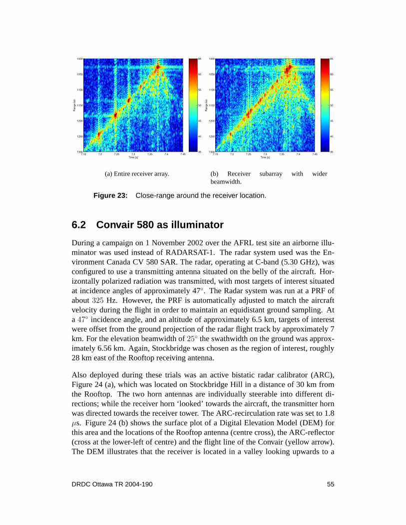
Time [s]

Ran

ge b

in

7.15 7.2 7.25 7.3 7.35 7.4 7.45

1000

1050

1100

1150

1200

1250

1300 35

40

45

50

55

60

65

(a) Entire receiver array.

Time [s]

Ran

ge b

in

7.15 7.2 7.25 7.3 7.35 7.4 7.45

1000

1050

1100

1150

1200

1250

1300 35

40

45

50

55

60

65

(b) Receiver subarray with widerbeamwidth.

Figure 23: Close-range around the receiver location.

6.2 Convair 580 as illuminator

During a campaign on 1 November 2002 over the AFRL test site an airborne illu-minator was used instead of RADARSAT-1. The radar system used was the En-vironment Canada CV 580 SAR. The radar, operating at C-band (5.30 GHz), wasconfigured to use a transmitting antenna situated on the belly of the aircraft. Hor-izontally polarized radiation was transmitted, with most targets of interest situatedat incidence angles of approximately 47◦. The Radar system was run at a PRF ofabout325 Hz. However, the PRF is automatically adjusted to match the aircraftvelocity during the flight in order to maintain an equidistant ground sampling. Ata 47◦ incidence angle, and an altitude of approximately 6.5 km, targets of interestwere offset from the ground projection of the radar flight track by approximately 7km. For the elevation beamwidth of25◦ the swathwidth on the ground was approx-imately 6.56 km. Again, Stockbridge was chosen as the region of interest, roughly28 km east of the Rooftop receiving antenna.

Also deployed during these trials was an active bistatic radar calibrator (ARC),Figure 24 (a), which was located on Stockbridge Hill in a distance of 30 km fromthe Rooftop. The two horn antennas are individually steerable into different di-rections; while the receiver horn ‘looked’ towards the aircraft, the transmitter hornwas directed towards the receiver tower. The ARC-recirculation rate was set to 1.8µs. Figure 24 (b) shows the surface plot of a Digital Elevation Model (DEM) forthis area and the locations of the Rooftop antenna (centre cross), the ARC-reflector(cross at the lower-left of centre) and the flight line of the Convair (yellow arrow).The DEM illustrates that the receiver is located in a valley looking upwards to a


hilly region. The flight line was chosen to resemble the rooftop-RADARSAT-1 ex-periment, i.e., a quasi-forward looking bistatic geometry. These trials were jointlycoordinated by DRDC Ottawa, Canada Centre for Remote Sensing (CCRS), andAFRL [42]. The rooftop receiver radar was working under the same conditions

(a) Photograph. (b) Surface plot of the DEM around AFRL,NY, (courtesy R. Hawkins et. al. [42]).

Figure 24: Photograph and location of active radar calibrator (ARC)at the 1 Nov. 2002 airborne trial, crosses) receiver andARC locations, arrow) flight path.

and with identical system parameters as for the RADARSAT trials. The airbornetransmitter, however, emits a non-linear frequency modulated pulse ofT = 7 µsduration and a bandwidth ofB = 50 MHz. However, since the low-pass filter inthe final stage of the receiver hardware (before sampling) limits the signal band-width to 30 MHz, a resolution loss will occur compared to the monostatic case. Forthese parameters, Fig. 25 shows the predicted maximum synthetic aperture timesand the ground range resolution, which indicate the poor range separability due tothe forward scattering geometry. Again, one of the first measured pulses was ex-tracted in order to compress all others in the range direction, Fig. 26 (a). The pulselength is7 µs long as expected. The magnitude and unwrapped phases history ofthe resulting compressed peaks of the direct path is plotted in Fig. 26 (b). The mag-nitude is the result of the multiplication of the two different antenna diagrams of thetransmitter and receiver. Due to the particular flight geometry the direct path signalis measured in sidelobe regions (both in azimuth and elevation) of the receiver andthe transmitter. Therefore, the two-way antenna pattern is not symmetric and showshigh sidelobes.

To re-order the continuous data stream into the range-time raw data array the vary-ing PRF has to be taken into account. The range migration corrected raw data field


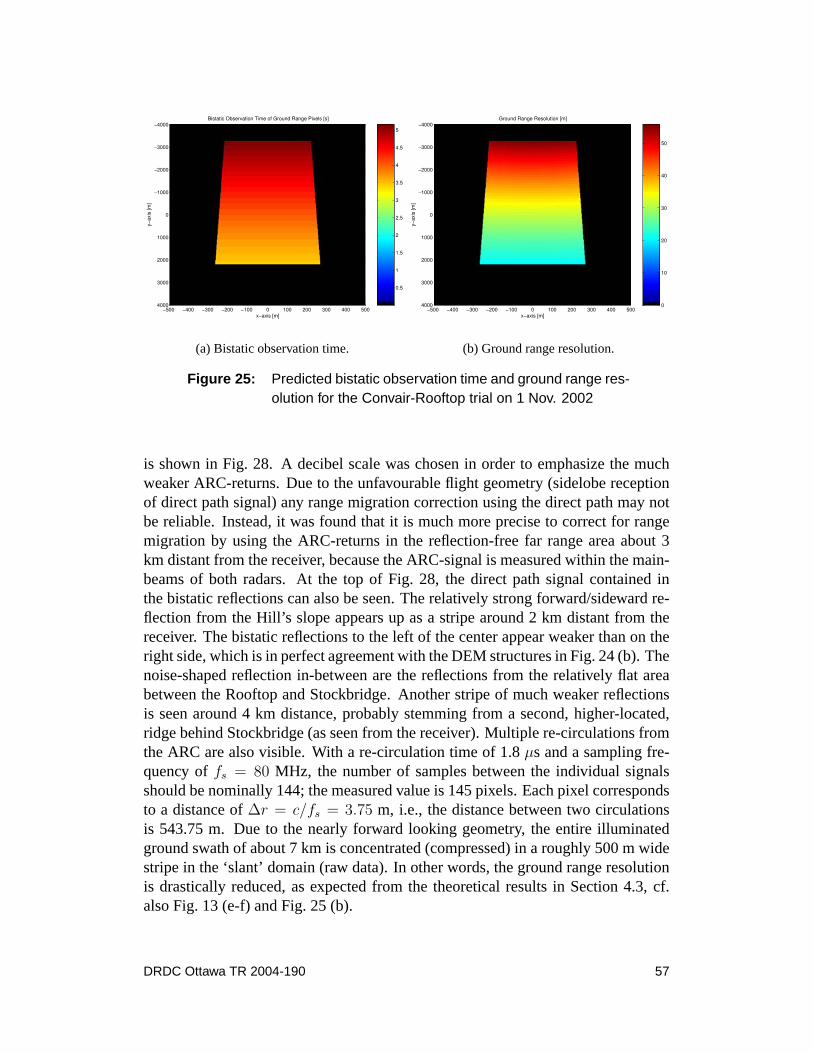
x−axis [m]

y−ax

is [m

]

Bistatic Observation Time of Ground Range Pixels [s]

−500 −400 −300 −200 −100 0 100 200 300 400 500

−4000

−3000

−2000

−1000

0

1000

2000

3000

4000

0.5

1

1.5

2

2.5

3

3.5

4

4.5

5

(a) Bistatic observation time.

x−axis [m]

y−ax

is [m

]

Ground Range Resolution [m]

−500 −400 −300 −200 −100 0 100 200 300 400 500

−4000

−3000

−2000

−1000

0

1000

2000

3000

4000 0

10

20

30

40

50

(b) Ground range resolution.

Figure 25: Predicted bistatic observation time and ground range res-olution for the Convair-Rooftop trial on 1 Nov. 2002

is shown in Fig. 28. A decibel scale was chosen in order to emphasize the muchweaker ARC-returns. Due to the unfavourable flight geometry (sidelobe receptionof direct path signal) any range migration correction using the direct path may notbe reliable. Instead, it was found that it is much more precise to correct for rangemigration by using the ARC-returns in the reflection-free far range area about 3km distant from the receiver, because the ARC-signal is measured within the main-beams of both radars. At the top of Fig. 28, the direct path signal contained inthe bistatic reflections can also be seen. The relatively strong forward/sideward re-flection from the Hill’s slope appears up as a stripe around 2 km distant from thereceiver. The bistatic reflections to the left of the center appear weaker than on theright side, which is in perfect agreement with the DEM structures in Fig. 24 (b). Thenoise-shaped reflection in-between are the reflections from the relatively flat areabetween the Rooftop and Stockbridge. Another stripe of much weaker reflectionsis seen around 4 km distance, probably stemming from a second, higher-located,ridge behind Stockbridge (as seen from the receiver). Multiple re-circulations fromthe ARC are also visible. With a re-circulation time of 1.8µs and a sampling fre-quency offs = 80 MHz, the number of samples between the individual signalsshould be nominally 144; the measured value is 145 pixels. Each pixel correspondsto a distance of∆r = c/fs = 3.75 m, i.e., the distance between two circulationsis 543.75 m. Due to the nearly forward looking geometry, the entire illuminatedground swath of about 7 km is concentrated (compressed) in a roughly 500 m widestripe in the ‘slant’ domain (raw data). In other words, the ground range resolutionis drastically reduced, as expected from the theoretical results in Section 4.3, cf.also Fig. 13 (e-f) and Fig. 25 (b).


−4 −3 −2 −1 0 1 2 3 4

x 10−6

−200

0

200

Pha

se [r

ad]

−4 −3 −2 −1 0 1 2 3 4

x 10−6

−50

0

50

Rea

l par

t

(a) Chirp signal; real part (red) and phase(blue).

−4 −3 −2 −1 0 1 2 3 4−4000

−3000

−2000

−1000

0

1000

Slow time [s]

Pha

se [r

ad]

−4 −3 −2 −1 0 1 2 3 40

1

2

3

4

5x 105

Mag

nitu

de

(b) Direct path signal; magnitude (red) andphase (blue).

Figure 26: Received chirp and direct path signals(magnitude and phase).

In order to compress the range-migration corrected data in the Doppler direction,the Doppler chirp rate must be known. Unfortunately, the motion data for the Con-vair aircraft were not available. Therefore, an autofocus method was used, basedon the phase information of the ARC in the far range. The magnitude and phasehistory of the ARC at 3 km range is plotted in Fig. 27 (a). While the magnitudeis quasi constant over a large region, the Doppler phase follows a typical parabolicshape. However, the apex of the Doppler phase is shifted off the center of the mag-nitude pattern, which is a clear indicator for the presence of a linear phase term,e.g., [40].

The technique to estimate the linear and quadratic phase coefficient of the matchedfilter is adopted from the moving target parameter estimation scheme described in[40]. There, the two coefficients are influenced by the along-track (quadratic term)and across-track (linear term) velocity of a moving object. One proposed techniqueto estimate these two components are matched filter banks; the desired parametersa = [a1, a2]

T are varied throughout a bank of filters of form

sref(t, a) = exp(j(a1t + a2t

2)), (105)

and the value at which the maximum output magnitude occurs represents the opti-mum estimate. Fig. 29 (a) shows the filter bank outputs for the chirp ratea2 variedbetween 50 s−2 and 200 s−2, where the linear terma1 was set to zero. The maxi-mum appears at a chirp rate of 121.4 Hz/s. The time at which this maximum occursis tc = 2.24 s, which represents the shifted (incorrect) position of the ARC in theSAR image. Again, this displacement is due the presence of the non-zero linear


−3 −2 −1 0 1 2 3

−2000

0

Slow time [s]

Pha

se [r

ad]

−4 −3 −2 −1 0 1 2 3 40

5000

10000

Mag

nitu

de

(a) Magnitude (green) and phase (blue).

0 1000 2000 3000 4000 5000 6000 700040

45

50

55

60

65

70

75

range [m]

[dB

]

(b) Magnitude of ARC-peaks.

Figure 27: Magnitude and phase of ARC-signal at 3 km range andmagnitudes of ARC-peaks along range.

terma1, which in terms of GMTI would correspond to non-zero radial or across-track velocity of the object. As known from the GMTI case, around the optimumchirp rate the matched filter responses shift away fromtc and broaden; the ridge istilted and fans out at the edges [40]. These effects are also caused by the mismatchof a1 in the matched filter and the data.

Slow time [s]

Ran

ge [m

]

−3 −2 −1 0 1 2 3

1000

2000

3000

4000

5000

6000

7000

0

10

20

30

40

50

Figure 28 : Range migration corrected raw data in logarithmic scale.


Analogously, a matched filter bank for the linear term componenta1 can be used.In order to avoid ambiguous impulse responses, the length of the reference functionshould not exceed the length of the target trajectory. For a matched filter bank mapwherea1 was varied from 0 to 1000 Hz, the maximum occurs ata1,opt = 895 Hz.Since the ARC was stationary, this frequency represents the difference of the localoscillators RF-frequencies|f1 − f2| = 895Hz.

Inserting this estimate into the reference function and repeating thea2 matchedfilter bank results in Fig. 29 (b). The ambiguity is resolved, i.e., only one peakoccurs; the ridge is now correctly shifted to the broadside timetb = −1.05 s andthe fan is straightened-out vertically. The impulse responses above the optimumvalue (abouta2 = 117 Hz/s) are not completely symmetric, which is caused bythe presence of non-zero cubic phase terms [43]. This term is most likely causedby uncompensated aircraft motion errors. A matched filter bank for the cubic term(not shown here) resulted ina3,opt = 1.16 Hz/s−2. Inserting the estimated phase

Slow time [s]

Chi

rp ra

te [s

−2]

−3 −2 −1 0 1 2 3

50

100

150

200

(a) Chirp rate.

Slow time [s]

Chi

rp r

ate

[s−2

]

−1.4 −1.3 −1.2 −1.1 −1 −0.9 −0.8 −0.7 −0.6

100

105

110

115

120

125

130

135

140

145

(b) Linear coefficient.

Figure 29: Matched filter banks for the chirp rate and the linearphase coefficient based on the ARC-signal in Fig. 27 (b).

coefficients into the reference function (105) and computing the convolution resultsin the bistatic SAR image shown in Fig. 30. All ARC-recirculations are correctlycompressed and appear as a “line of dots” in the centre of the SAR image. Thelinearly decreasing magnitude (in dB scale) along range is confirmed in Fig. 27 (b).

Due to the very small ground range resolution details, such as streets, buildingsfields etc. in the Stockbridge area are not recognizable However, by comparingFig. 31 and the DEM in Fig. 24 (b), certain patterns in the slope structures (differentridges) in the DEM show up as reflections. Further, some compression gain isobservable in the relatively flat region between the receiver and Stockbridge Hill.


Slow time [s]

Ran

ge [m

]

−3 −2 −1 0 1 2 3

1000

2000

3000

4000

5000

6000

7000

Figure 30 : Bistatic SAR image for the 1 Nov. 2002 airborne trial.

Slow time [s]

Ran

ge [m

]

−3 −2 −1 0 1 2 3

1400

1600

1800

2000

2200

2400

2600

Figure 31 : Bistatic SAR image for the 1 Nov. 2002 airborne trial aroundARC location.


6.3 Measured phase noise characteristics

This section investigates the phase noise characteristics measured during the bistaticclutter experiments at AFRL described in subsections 6.1 and 6.2. Since the directpath signal between the moving transmitter and the stationary receiver was ob-served, it is possible to explore the phase noise properties under practical conditionsand to verify the theoretical results introduced in Section 2.3.

6.3.1 Rooftop-RADARSAT-1 experiment

Figure 32 (a) shows the direct-path signal phase along Doppler-direction (bluecurve). This phase, confined to the area underneath the mainbeam (T = 6.9 s to 8s), is given as the integral over the Doppler frequency plotted in Fig. 20 (a) (red).The green and the red curves show the residual phase after removing a second andthird order polynomial fit from the Doppler phase. As expected, the satellite showsonly small motion error induced phase deviations (e.g., a relatively small cubicterm) over the synthetic aperture time ofTs = 1.1 seconds. The IISLR for the twocurves are -15.3 dB and -19.3 dB according to Table 2, and hence, are getting closeto the requirement of -20 dB. Figure 32 (b) confirms this finding by plotting the

0 0.2 0.4 0.6 0.8 10

300

600

900

1200

time [s]

Dop

pler

pha

se [r

ad]

0 0.2 0.4 0.6 0.8 1−1

−0.5

0

0.5

1

Pha

se n

oise

[rad

]

(a) Doppler phase (blue) and phase noise(red, green).

0.5 0.55 0.6 0.65−60

−50

−40

−30

−20

−10

0

time [s]

Poi

nt s

prea

d fu

nctio

n [d

B]

(b) PSF, ideal (blue), noisy (red).

Figure 32: Measured phase noise of Rooftop-RADARSAT-1 experiment and im-pact on point spread function.

point spread functions with and without the shown phase noise residual. The bluecurve represents the undisturbed PSF for the estimated polynomial coefficients, i.e.,the fitted Doppler rate. The red curve indicates the PSF when the residual noise(green) is added to the signal and then compressed with the undisturbed matched


filter. Only a slight one-sided increase of the peak sidelobe is observed due to theremaining cubic phase error but virtually no increase in ISLR.

6.3.2 Rooftop-Convair 580 experiment

For the airborne illuminator, the scenario is entirely different. Since no motioncompensation on the data was performed due to non-availability of the INS/GPSaircraft data, motion induced phase errors (caused by deviations from a perfectlystraight flight line and constant velocity) will be superimposed on the oscillatorphase noise. Figure 33 (a) shows the residual phase noise in the direct path signalover eight seconds after removal of quadratic and cubic polynomial fits from themeasured Doppler phase (blue curve) in Fig. 26 (b). A much larger standard de-viation of 1.16 rad and 0.75 rad, respectively is seen (these values are too large toallow computation of the IISLR via (37)).

The drastic impact on the PSF, even for the third order phase noise residual, isvisible in Fig. 33 (b). Alongside a significant increase of the peak sidelobes, aleft-sided increase of the side lobes and an increased ISLR are recognized. Whilethe one-sided sidelobe increase points to unresolved higher-order low-frequencyphase noise terms, the two peak sidelobes occur as ghost targets, which might becaused by the sinusoidal, low-frequency structure in Fig. 32 (a), [24]. However, this

0 1 2 3 4 5 6 7 8−2.5

−2

−1.5

−1

−0.5

0

0.5

1

1.5

2

time [s]

Pha

se n

oise

[rad

]

quadraticcubic

(a) Phase noise.

3.2 3.4 3.6 3.8 4 4.2 4.4 4.6 4.8−60

−50

−40

−30

−20

−10

0

time [s]

Poi

nt s

prea

d fu

nctio

n [d

B]

(b) PSF, ideal (blue), noisy (red).

Figure 33: Measured phase noise of Rooftop-Convair 580 experiment and im-pact on point spread function.

situation improves substantially for shorter coherent processing times. For instance,halving this time toTs = 4 s leads to much smaller standard deviations, i.e., toIISLRs of -14.2 dB and -19.7 dB, respectively. Correspondingly, the PSF for four


seconds (third order polynomial fit) is almost undistinguishable from the blue curvein Fig. 33 (b) and is therefore not plotted.

Even though the motion error induced phase noise and the oscillator phase noisecontributions are inseparable without proper INS data, Fig. 34 reveals some deeperinsight. Here, the estimated power spectral density after removal of up to secondorder or third order polynomial fits is plotted within the unambiguous frequencyband (PRF = 325 Hz). The Fourier transform reveals discrete phase noise at about72 Hz, which are known to be caused by propeller shaft vibrations of the Convair580. The other spikes at about 30 Hz, 120 Hz and 180 Hz are probably due to framevibrations of the aircraft (due to under-sampling of the azimuthal bandwidth, someare most likely ambiguous frequencies folded back into the PRF-region). Thesevibrations cause the oscillator to shake, which in turn will perturb the oscillatorfrequency (phase) due to its ‘g-sensitivity’. A detailed, experiment based, analysisof motion and vibration induced phase jitter and the resultant limitations on thecoherent processing time will be performed during phase II of this TIF project.

−150 −100 −50 0 50 100 150−80

−70

−60

−50

−40

−30

−20

−10

0

10

Frequency [Hz]

Pow

er s

pect

ral d

ensi

ty [d

B]

quadraticcubic

Figure 34 : Power density spectrum of phase noise for Rooftop-Convair 580experiment.

In contrast, the estimated power spectral density for the RADARSAT-1-Rooftopexperiment shows no such spikes, as expected.


7 Bistatic SAR processing

Finding fast and reliable processing algorithms for the geometrically more demand-ing bistatic configuration is a relatively open field of research at present. Somework on this field had been reported in the early papers by Soumekh [44, 45, 46]and others [47, 48]. However, to date, most bistatic SAR processors are based onthe matched filter principle and are, in fact, solely time domain correlators [49, 50].Time domain correlation or convolution is universally applicable to any bistaticconfiguration (including monostatic) and is relatively simple to implement. Forthese reasons we have adopted the matched filter processor that is described in thissection. Future work will certainly include investigation of alternative processors.

The major drawback of the time domain technique is the enormous computationalload involved that leads to intolerable processing times. Unlike monostatic SAR,the kernel function for bistatic cases is non-separable and, hence, the use of fastoperators such as the Fast Fourier Transform (FFT) is prevented, [16]. Recently,Ender [51] explored the theoretical background of bistatic Doppler compressionand has proposed numerical methods to separate the kernel. Some useful analyticexpressions for bistatic geometry can also be found in [17]

Let us assume that the bistatic geometrical history is accurately known, for instance,by measurements from Global Positioning System (GPS), differential GPS, andIntegrated Inertial System (INS) equipment on-board the platforms. Then, the rangeand Doppler history of any scatterer (location) on the bistatically observed groundis a-priori known. In other words, the range trajectory of a particular scatterercan be predicted within the two-dimensional raw data field, including the rangewalk and range migration, see Fig. 35. Note that the range-trajectory for a bistaticSAR is generally not a parabola as compared to the monostatic case. The shadedareas around the tracks represent the duration of the transmitted pulses. After rangecompression, which is done identically to the monostatic case, this shaded regionis compressed down to a narrow line, where the width of the line is determined bythe range-resolution of the system, see Section 4.3.

To fully identify the individual scatterer tracks in the raw-data array, a precise timekeeping is required for the range gating. In other words, one must be able to assignthe exact bistatic distance (near-range) to the time when the range gates are openedat the receiver. Since illuminator and receiver are spatially separated, this is equiva-lent to a non-trial synchronisation issue. Time synchronisation can actually be donedirectly, i.e., with an extra link between the transmitter and receiver, or indirectlyusing identical stable clocks. The first technique was applied during the bistaticclutter trials described in Chapter 6.


+

+

+

slow time

bistatic ran

ge

Figure 35 : Illustration of a bistatic raw data field (right) showing three individ-ual range trajectories for scatterer locations specified in the illumi-nated footprint on the ground (left).

Indirect time synchronisation for range-gating based on the pulse-per-second (PPS)signal of the GPS offers greater flexibility to use in future systems as well as reducedhardware changes on the existing aircraft [21, 28]. As such it is intended for theexperimental set-up in phase II of this project. However, the fewer modifications tothe hardware have to be traded with less accuracy, i.e., a larger uncertainty in therange cell position; this error is expected to be less than ten ns.

By examining Fig. 35, the task of how to compress the energy for each image pixelbecomes clear; one must re-collect the spread energy along the a priori known tra-jectories. This is done by convolving the measured data along the trajectory withthe theoretical slow-time signal (matched filter) created by a potential scatterer at aparticular location in the image. A slightly different way of executing this Dopplerprocessing is referred to as Algorithm 1, as described in appendix G. Here, for eachrange-line (pulse return), a complete image is computed. The ensemble of imagesare then subsequently added coherently. The energy of the echoes of each pulse aredistributed throughout the image according to the a priori known distance betweenimage pixels and the platform positions. The introduced algorithm has been imple-mented and tested on the experimental bistatic clutter data from 28 January 2002,as described in Section 6.1.

Figure 36 shows the Doppler focussed image for a small area around StockbridgeHill. Three sperate scattering centers along a quasi-straight line can be seen alongwith their ghost replicas. In order to understand this phenomenon, three equi-Doppler (red) and equi-range (yellow) lines are superimposed onto the image. Ev-idently the ghost images appear exactly at the intersections of these lines, confirm-ing ambiguous echoes caused by the quasi forward looking geometry. Scatterers at


these locations (intersection points) would generate exactly identical slow time his-tories in range and Doppler, i.e., would exactly lay on top of each other in Fig. 35and possess identical Doppler histories. Further details of this algorithm and itsproperties can be found in [52].

In contrast, the same kind of ghost images did not appear in Fig. 23 since a directconvolution with the estimated Doppler history (chirp signal) was applied, whichwill produce only one single match whenever the matched filter lines up exactlywith the measure data. However, the technique used in Section 6 is only a crudeapproximation because the range migration correction was assumed constant overthe entire image, but therefore is about one-hundred times faster.

Latit

ude

[N]

Longitude [W]75.816 75.765 75.714 75.663 75.613 75.562 75.511 75.460 75.410

43.2006

43.1672

43.1338

43.1004

43.067

43.0336

43.0002

42.9668

42.93340

5

10

15

20

25

30

Figure 36 : SAR image processed with algorithm one and overlayed equi-range and equi-Doppler lines for three strong scatterers.


8 Summary and outlook

This report described the results of phase I of the TIF project on bistatic SAR.This phase lasted one year and was concerned with gaining a deeper knowledge ofbistatic SAR and a thorough understanding of its properties based on theoreticalanalysis as well as analysis of existing experimental space-borne and airborne SARdata sets.

A complete theoretical framework for the bistatic SAR resolution on the groundwas developed. Using this mathematical tool, the range and Doppler ground res-olution can be predicted for any arbitrary bistatic flight geometry. By using thetime-dependent range and Doppler gradients and the bistatic observation time, thiscan be achieved without actually calculating the point spread or impulse responsefunction, which makes it computable in quasi real-time. In addition, due to theirsimplicity, this set of equations can be used for mission planing where the optimumflight lines must be determined in order to achieve a minimum required resolutionfor a given area of interest. Further, performance degradation in terms of reducedgeometric and radiometric resolution of the point spread function caused by severephase noise due to separate oscillators was investigated.

In order to verify these theoretical results a complete bistatic raw data simulator hasbeen developed and implemented in MATLABc©. The simulator generates the rawdata with high accuracy including the full three-dimensional geometry, the antennadiagrams, and the complex RCS for any number of point scatterers located on theground. Hence, realistic effects such as range migration and magnitude weight-ing are automatically included. A more practical scene including features suchas streets, fields etc., could be assembled from an ensemble of point scatterers.However, the computational complexity increases drastically in proportion to thenumber of scatterers. The simulator also allows antenna squinting, as is commonlydone in special SAR modes such as SlideSAR and SpotSAR.

The simulated raw data are used to test the performance of bistatic SAR processingalgorithms. In particular, a ‘brute force’, time domain SAR processor was intro-duced in Section 7. Although this type of processor is very time consuming, it isbased on the matched filter approach and is, therefore, flexible and applicable toany complex geometry.

The last part of the report dealt with the analysis of experimental data collectedat bistatic clutter trials at Rome, NY throughout 2002. These trials comprised amoving transmitter (either the RADARSAT-1 satellite or the Environment CanadaConvair-580 aircraft) and a stationary receiver antenna located on the premises ofAFRL. Since the main motivation for those trials was to collect and build-up databases for bistatic clutter properties and bistatic GMTI a relatively narrow receiver


antenna beamwidth was sufficient. However, due to the relative motion betweenthe two separate radars, these data sets are in principle also suitable for Dopplerprocessing, i.e., bistatic compression/focussing in the ‘cross-range’ direction to en-hance the resolution. Although no special measures were taken to ensure phasecoherence between transmitter and receiver, i.e., the two stable local oscillatorswere running freely during the measurements, both data sets have successfully beenfocussed to the theoretically expected resolutions. This was mainly due to the rela-tively small synthetic aperture times of up to only a few seconds in both cases.

In Phase II of the project, deeper insight into the functionality of a bistatic SAR sys-tem and the physical properties of its SAR imagery will be gained by experimentalmeasurements conducted by DRDC Ottawa’s airborne SpotSAR radar system. De-signing and constructing a secondary receiver which will be placed on top of astationary platform (e.g., a tower or a high building) and locating the transmitter onthe maneuvering aircraft, represents the simplest useful bistatic configuration andis of particular interest for evaluating the performance limits for scenarios with-out any receiver platform motions. Indirect time synchronisation for range-gatingbased on the pulse-per-second (PPS) signal of the global positioning system (GPS)is intended for the experimental set-up because of the reduced hardware changes onthe existing aircraft. The received echoes from the illuminated ground spot wouldbe recorded and stored for off-line processing. Flight trials with different bistaticgeometries and varying imaged scenarios, such as different vegetation or importedman-made targets (cars etc.), are anticipated to be conducted during phase II of theproject.


References

1. Willis, N. J. (1995). Bistatic Radar, 2 ed. Silver Spring, MD: TechnologyService Corporation.

2. Willis, N. J. (2002). Bistatic Radars and Their Third Resurgence: PassiveCoherent Location. IEEE Radar Conference Tutorial 2.1.

3. Retzer, G.. (1980). A Concept for Signal Processing in Bistatic Radar. InIEEEInt. Radar Conference, pp. 288–293.

4. Kirk Jr., J. C. (1985). Bistatic SAR Motion Compensation. InIEEEInternational Radar Conference, pp. 360–365. New York, USA.

5. Ferrazzoli, P., Guerriero, L., DelMonaco, C. I., and Solimini, D. (2003). Afurther inside into the potentials of bistatic SAR in monitoring the earthsurface. InProc. of IGARSS’03, Toulouse, France.

6. Moccia, A., Rufino, G., and De Luca, M. (2003). Oceanographic Applicationof Spaceborne Bistatic SAR. InProc. of IGARSS’03, Toulouse, France.

7. Krieger, G., Fiedler, H., Hounam, D., and Moreira, A. (2003). Analysis ofSystem Concepts for Bi- and Multistatic SAR Missions. InProc. ofIGARSS’03, Toulouse, France.

8. Krieger, G., Fiedler, H., Hounam, D., and Moreira, A. (2003). Bi- andMulti-Static SAR Missions: Potentials and Challenges. In Agency,Canadian Space, (Ed.),Advanced SAR Workshop, Saint-Hubert, Quebec,Canada.

9. Eineder, M. (2003). Oscillator Clock Drift Compensation in BistaticInterferometric SAR. InProc. of IGARSS’03, Toulouse, France.

10. Cerutti-Maori, D. and Ender, J. H. G. (2003). An Approach to MultistaticSpaceboren SAR/MTI Processing and Performance Analysis. InProc. ofIGARSS’03, Toulouse, France.

11. Whitewood, A. P., Muller, B.R., Griffiths, H. D., and Baker, C. J. (2003).Bistatic Synthetic Aperture Radar with Application to Moving TargetDetection. InInternational Conference on Radar, pp. 529–534. Adelaide,Australia.

12. Pileih, C. and Beard, J. K. (2000). Bistatic GMTI experiment for airborneplatforms. InIEEE International Radar Conference, pp. 42–46. Washington,D.C.


13. Cazzani, L., Colesanti, C., Leva, D., Nesti, G., Prati, C., Rocca, F., and Tarchi,D. (2000). A Ground-Based Parasitic SAR experiment.IEEE Trans.Geoscience and Remote Sensing, GRS-38(5), 2132–2141.

14. Retzer, G.. (1979). A Passive Detection System for a Wide Class of IlluminatorSignals. InProc. IEEE Int. Conf. Acoust., Speech, Signal Processing, pp.620–623. Washington, D.C.

15. Homer, J., Mojarrabi, B., Palmer, J., Kubic, K., and Donskoi, E. (2003).Non-cooperative Bistatic SAR Imaging System: Spatial Resolution Analysis.In Proc. of IGARSS’03, Toulouse, France.

16. Ender, J. H. G. (2003). Signal Theoretical Aspects of Bistatic SAR. InProc. ofIGARSS’03, Toulouse, France.

17. Loffeld, O., Nies, H., Peters, V., and Knedlik, S. (2003). Models and UsefulRelations for Bistatic SAR Processing. InProc. of IGARSS’03, Toulouse,France.

18. Gierull, C. H. and Sikaneta, I. (2004). Ground Moving Target ParameterEstimation for Two-Channel SAR. InProc. of EUSAR, pp. 799–802. Ulm,Germany.

19. Adams, J. W. and Schifani, T. M. (1987). Waveform Error Analysis for BistaticSynthetic Aperture Radar Systems. InInter. Radar Conf., pp. 479–483.London, UK.

20. Massonnet, D. and Vadon, H. (1995). ERS-1 Internal Clock Drift Measured byInterferometry.IEEE Trans. Geoscience and Remote Sensing, GRS-33(2),401–408.

21. Weiß, M. (2003). EBiRa: Experimental Bistatic Radar for air surveillance. InProc. of IGARSS’03, Toulouse, France.

22. Rutman, J. and Walls, F. L. (1991). Characterization of Frequency Stability InPrecision Frequency Sources.Proc. of the IEEE, 79(6), 952–960.

23. Auterman, J. L. (1984). Phase Stability Requirements for a bistatic SAR. InProc. IEEE Int. Radar Conf., pp. 48–52. Atlanta, GA.

24. Carrara, W. G., Goodman, R. S., and Majewski, R. M. (1995). SpotlightSynthetic Aperture Radar, Artech House.

25. Allan, D. W. (1987). Time and Frequency (Time-Domain) Characterization,Estimation, and Prediction of Precision Clocks and Oscillators.IEEE Trans. onUltrasonics, Ferroelectrics, and Frequency Control, 34(6), 647–654.


26. Cutler, L. S. and Searle, C. L. (1966). Some Aspects of the Theory andMeasurment of Frequency Fluctuations in Frequency Standards.Proc. ofIEEE, 54(2), 136–154.

27. Damini, A, Haslam, G., Balaji, B., and Goulding, M. (2004). A new X-bandExperimental Airborne Radar for SAR and GMTI. InProc. of EUSAR, pp.639–642. Ulm, Germany.

28. Weiß, M. (2004). Time and Frequency Synchronisation Aspects for BistaticSAR. InProc. of EUSAR, Ulm, Germany.

29. Bohme, J. F. (1993). Stochastische Signale, Stuttgart: Teubner-Verlag.

30. Papoulis, A. (1991). Probability, Random Variables and Stochastic Processes,3 ed. McGraw Hill Inc.

31. Ender, J. H. G. (1991). Analyse der Selbstfokussierung eines Radars mitsynthetischer Apertur (SAR) unter Verwendung einer Gruppenantenne. Ph.D.thesis. Ruhr-Universit”at Bochum.

32. Snarski, C. A. (1994). A phase error estimation algorithm: theory, application,and examples. InProc. of the SPIE, Vol. 2230, pp. 72–86. Orlando, FL.

33. Ender, J. H. G. (2001). The Meaning of K-Space for Classical and AdvancedSAR-Techniques. InProc. of PSIP, pp. 1–13. Marseilles.

34. Cardillo, C.P. (1990). On the Use of the Gradient to Determine Bistatic SARResolution. InProc. of Int. Symp. Antennas and Propagation, Vol II, pp.1032–1035. Dallas, TX.

35. Walterscheid, I., Brenner, A. R., and Ender, J. H. G. (2004). Geometry andStystem Aspects for a Bistatic Airborne SAR-Experiment. InProc. of EUSAR,pp. 567–570. Ulm, Germany.

36. Chiron, O. (1997). Analysis of bistatic synthetic aperture radar images. InKAG-15, (Ed.),Participation in Space Based Radar Experiments (FinalReport), The Technical Cooperation Program (TTCP).

37. I., Walterscheid, Brenner, A. R., and Ender, J. H. G. (2004). Results on bistaticsynthetic aperture radar.Electronics Letters, 40(19), 1224–1225.

38. Livingstone, C., Sikaneta, I., Gierull, C. H., Chiu, S., Beaudoin, A., Campbell,J., J., Beaudoin, Gong, S., and Knight, T. (2002). An Airborne SARExperiment to Support RADARSAT-2 GMTI.Canadian J. Remote Sensing,28(6), 1–20.


39. Tunaley, J. and Cotuk, N. (2004). Analysis of Bistatic Radar Data Collected byAFRL on 28 Jan. 02. (Technical Report TR 2004-xxx). Defence R&D Canada– Ottawa. Canada.

40. Gierull, C. H. and Livingstone, C. (2004). SAR-GMTI Concept forRADARSAT-2. In Klemm, R., (Ed.),The Applications of Space-TimeProcessing, Stevenage, UK: IEE Press.

41. Gierull, C. H. and Sikaneta, I. (2003). Raw Data Based Two-Aperture SARGround Moving Target Indication. InProc. of IGARSS’03, Toulouse, France.

42. Hawkins, R., Murnaghan, K. P., Wind, A., Nedelcu, S., and Choeurng, V.(2003). Monostatic SAR Summary from Rome NY Novenmber 1, 2002.(Technical Note CCRS-TN 2003-06). Canada Centre for Remote Sensing.Canada.

43. Sharma, J. (2004). The influence of target acceleration on parameter estimationand focusing in SAR imagery. Master’s thesis. University of Calgary.

44. Soumekh, M. (1991). Bistatic Synthetic Aperture Radar Inversion withApplication in Dynamic Object Imaging.IEEE Trans. Signal Processing,39(9), 2044–2055.

45. Soumekh, M. (1998). Wide-Bandwidth Continous-Wave Monostatic/BistaticSynthetic Aperture Radar Imaging. InInter. Conference on Image Processing,pp. 361–364. Chicago, IL.

46. Soumekh, M. (1998). Bistatic Synthetic Aperture Radar Imaging UsingWide-Bandwidth Continous-Wave Sources. InSPIE Conference on RadarProcessing Technology and Applications III, Vol. 3462, pp. 99–109. SanDiego.

47. Arikan, O. and Munson Jr., D. C. (1988). A Tomographic Formulation ofBistatic Synthetic Aperture Radar. InInter. Conf. on Advances inCommunication and Control Systems, pp. 289–302. Baton Rouge.

48. Ding, Y. and Munson Jr., D. C. (2002). A Fast Back-Projection Algorithm forBistatic SAR Imaging. InIEEE Inter. Conf. on Image Processing, New York.

49. Cantalloube, H., Wendler, M., Giroux, V., Dubois-Fernandez, P., and Krieger,G. (2004). Challenges in SAR processing for airborne bistatic acquisition. InProc. of EUSAR, pp. 577–580. Ulm, Germany.

50. Yates, G., Horne, M., Blake, A. P., Middleton, R., and Andre, D. B. (2004).Bistatic SAR image formation. InProc. of EUSAR, pp. 581–584. Ulm,Germany.


51. Ender, J. H. G. (2004). A Step to Bistatic SAR Processing. InProc. of EUSAR,pp. 359–363. Ulm, Germany.

52. Cotuk, N. and Gierull, C. H. (2004). Time Domain Bistatic SAR Processor.(Technical Report TM 2004-000). Defence R&D Canada - Ottawa.

53. Golub, G. H. and Van Loan, C. F. (1989). Matrix Computations, Baltimore:Johns Hopkins University Press.

54. Ender, J. H. G (1999). Konventionenuber Koordinatensysteme etc. FGANInternal Note.


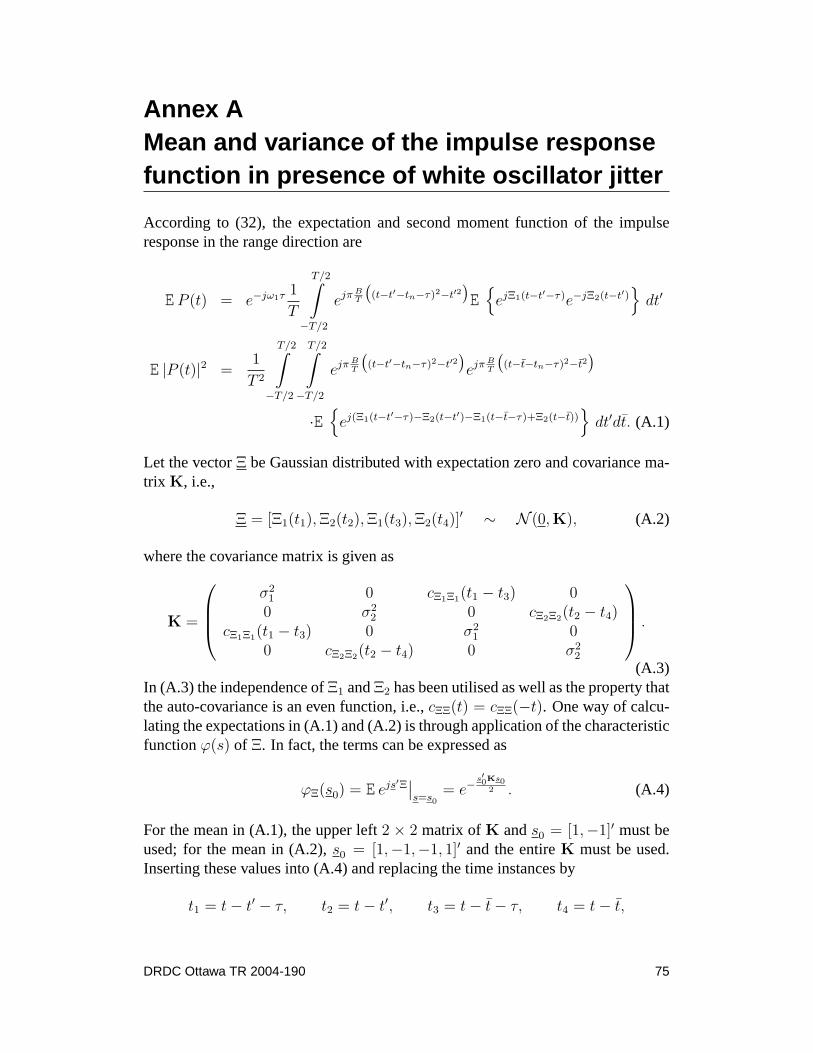
Annex AMean and variance of the impulse responsefunction in presence of white oscillator jitter

According to (32), the expectation and second moment function of the impulseresponse in the range direction are

EP (t) = e−jω1τ 1

T

T/2∫−T/2

ejπ BT

((t−t′−tn−τ)2−t′2

)E{

ejΞ1(t−t′−τ)e−jΞ2(t−t′)}

dt′

E |P (t)|2 =1

T 2

T/2∫−T/2

T/2∫−T/2

ejπ BT

((t−t′−tn−τ)2−t′2

)ejπ B

T

((t−t−tn−τ)2−t2

)·E{

ej(Ξ1(t−t′−τ)−Ξ2(t−t′)−Ξ1(t−t−τ)+Ξ2(t−t))}

dt′dt. (A.1)

Let the vectorΞ be Gaussian distributed with expectation zero and covariance ma-trix K, i.e.,

Ξ = [Ξ1(t1), Ξ2(t2), Ξ1(t3), Ξ2(t4)]′ ∼ N (0,K), (A.2)

where the covariance matrix is given as

K =

σ2

1 0 cΞ1Ξ1(t1 − t3) 00 σ2

2 0 cΞ2Ξ2(t2 − t4)cΞ1Ξ1(t1 − t3) 0 σ2

1 00 cΞ2Ξ2(t2 − t4) 0 σ2

2

.

(A.3)In (A.3) the independence ofΞ1 andΞ2 has been utilised as well as the property thatthe auto-covariance is an even function, i.e.,cΞΞ(t) = cΞΞ(−t). One way of calcu-lating the expectations in (A.1) and (A.2) is through application of the characteristicfunctionϕ(s) of Ξ. In fact, the terms can be expressed as

ϕΞ(s0) = E ejs′Ξ∣∣s=s0

= e−s′0Ks0

2 . (A.4)

For the mean in (A.1), the upper left2 × 2 matrix of K ands0 = [1,−1]′ must beused; for the mean in (A.2),s0 = [1,−1,−1, 1]′ and the entireK must be used.Inserting these values into (A.4) and replacing the time instances by

t1 = t− t′ − τ, t2 = t− t′, t3 = t− t− τ, t4 = t− t,


yields

EP (t) = e−σ21+σ2

22 e−jω1τ 1

T

T/2∫−T/2

ejπ BT

((t−t′−tn−τ)2−t′2

)dt′, (A.5)

and hence

|EP (t)| = e−σ21+σ2

22 sinc(πB(t− tn − τ)). (A.6)

For the second moment function we get

E |P (t)|2 = e−(σ21+σ2

2) 1

T 2

T/2∫−T/2

T/2∫−T/2

ejπ BT

(t−tn−τ)(t′−t)ecΞ1Ξ1(t′−t)+cΞ2Ξ2

(t′−t) dt′dt.

(A.7)Under the assumption of identical oscillatorscΞ1Ξ1(t) = cΞ2Ξ2(t) ≡ cΞΞ(t), (A.7)can be rewritten as

E |P (t)|2 = e−2σ2 1

T 2

T/2∫−T/2

T/2∫−T/2

ejπ BT

(t−tn−τ)(t′−t)(e2cΞΞ(t′−t) − 1

)dt′dt

+e−2σ2 1

T 2

T/2∫−T/2

T/2∫−T/2

ejπ BT

(t−tn−τ)(t′−t) dt′dt. (A.8)

Providing statistically white phase noise, i.e.,cΞΞ(t) = σ2δ(t), whereδ(t) denotesthe Dirac delta function , the first integrand on the right hand side of (A.8) becomesthe line integral

e−2σ2

T 2

T/2∫−T/2

(e2σ2 − 1

)√2 dt (A.9)

so that

E |P (t)|2 =

√2

Te−2σ2

(e2σ2 − 1

)+ e−2σ2

sinc2(πB(t− tn − τ)), (A.10)

and hence, with (A.5),

σ2p(t) = E |P (t)|2 − |EP (t)|2 =

√2

T

(1− e−2σ2

). (A.11)


Annex BStandard deviation of phase noise for a finiteobservation time

Let Ξ(t) denote a wide sense stationary stochastic and ergodic phase noise processwith variance

σ2Ξ = E (Ξ(t)− EΞ(t))2 = EΞ(t)2 − (EΞ(t))2 , (B.1)

which describes the variation of the phase around its mean of zero for an infiniteobservation time. We are now interested in the variation of this phase process (vari-ance) for finite observation timesT . For a given realisationξ(t) of the stochasticprocess measured over timeT ′ � T , we can estimate this variance as the averageof the differences〈(ξT (t)− ξT (t))2〉 within the observation intervalT . Sliding theobservation window along the time axis we can see how this (time-limited) varianceestimate varies over time, see Fig. B.1.

t’

t

T

1/T

Figure B.1 : Realisation of phase noise with sliding window to estimate the rmsfor finite observation time T .

Mathematically, this can be expressed as the convolution of the phaseξ(t) and theideal low-pass filterh(t) = 1/T rect(t/T ), i.e.,

σ2ξ (t, T ) =

1

Tξ(t)2 ∗ rect

(t

T

)− 1

T 2

(ξ(t) ∗ rect

(t

T

))2

, (B.2)

where∗ represents the convolution operator. The mean value of this variance func-tion over the entire measurement timeT ′ is

σ2ξ (T ) =

1

T ′

T ′/2∫−T ′/2

σ2ξ (t, T ) dt, (B.3)

which may be used as a measure of the rms phase noise for limited observationtime. Applying the Fourier-transform to (B.2) and inserting the result into (B.3),


including the inverse Fourier-transform, yields

σ2ξ (T ) =

1

T ′

T ′/2∫−T ′/2

∞∫−∞

(Ξ(ω) ∗ Ξ(ω)) sinc (ωT/2) exp(jωt) dω dt (B.4)

− 1

T ′

T ′/2∫−T ′/2

∞∫−∞

(Ξ(ω) sinc (ωT/2)

)∗(Ξ(ω) sinc (ωT/2)

)exp(jωt) dω dt,

whereΞ(ω) denotes the Fourier-transform ofξ(t) (not to be confused with thestochastic process) andT sinc(ωT/2) is the corresponding Fourier-transform of therectangular window. Switching the integration order and using the Dirac-functionapproximation gives

1

T ′

T ′/2∫−T ′/2

exp(jωt) dt = sinc (ωT ′/2) ∼= δ(ω) for T ′ � 1 (B.5)

and writing out the convolution integral leads to

σ2ξ (T ) =

∞∫−∞

∞∫−∞

Ξ(ω − ν)Ξ(ν) dν sinc (ωT/2) δ(ω) dω (B.6)

−∞∫

−∞

∞∫−∞

Ξ(ω − ν) sinc ((ω − ν)T/2) Ξ(ν) sinc (νT/2) dν δ(ω) dω.

Exploiting the ‘sifting property’ of the Dirac-function and the fact thatΞ(ω) =Ξ(−ω)∗, we can write

σ2ξ (T ) =

∞∫−∞

|Ξ(ω)|2(1− sinc (ωT/2)2) dω. (B.7)

In order to investigate the statistical properties of the estimator (B.7), e.g., the ex-pectation value, we cannot simply replace the realisationξ(t) with the correspond-ing random process because the Fourier-transform of a stationary stochastic process(which has infinite energy) does not exist. However, substituting the finite Fouriertransform in (B.4) by the discrete Fourier transform

ξn =1

N

N−1∑k=0

Ξk exp (j2πnk/N) (B.8)


and following the time-continuous derivation above, leads to

σ2ξ (K) =

1

N

N−1∑k=0

|Ξk|2(1− sinc2 (πkK)

)=

N−1∑k=0

INΞΞ(k)

(1− sinc2 (πkK)

),

(B.9)whereIN

ΞΞ(k) denotes the periodogram of lengthN . It is well known that the expec-tation of the periodogram for sufficiently largeN is identical to the power densityspectrum ofΞ, i.e.,E IN

ΞΞ(k) = CΞΞ(k) [30]. Finally, in time continuous notation,the variance can be computed as

σ2Ξ =

∞∫−∞

CΞΞ(ω)(1− sinc2 (ωT/2)

)dω ∼= 2

∞∫0.443

T

CΞΞ(ω) dω, (B.10)

where the sinc-function has been approximated by a rectangular window with a3dB-width of0.443/T .

Alternatively, the same result can be calculated as the expectation of

σ2 = E

1

T

∞∫−∞

∣∣∣∣∣∣Ξ(t)− 1

T

∞∫−∞

Ξ(s) ds

∣∣∣∣∣∣2

dt

, (B.11)

where both integrals of stochastic processes are defined as ‘mean square’ integrals.


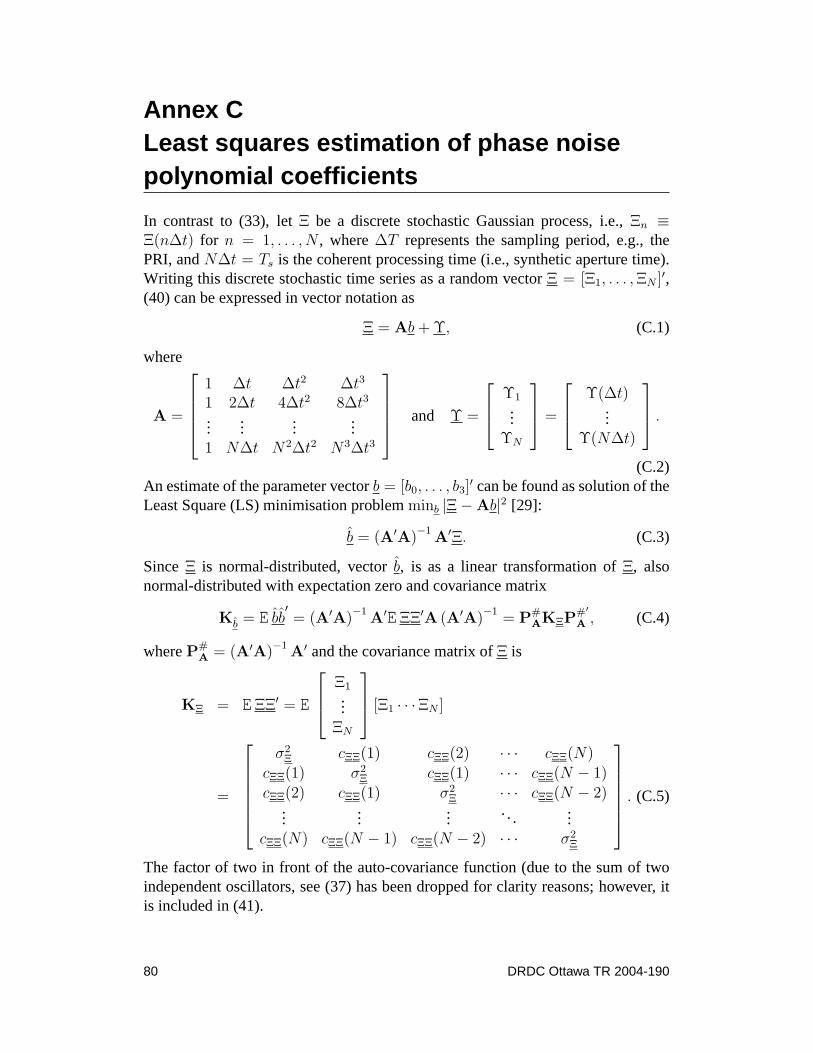
Annex CLeast squares estimation of phase noisepolynomial coefficients

In contrast to (33), letΞ be a discrete stochastic Gaussian process, i.e.,Ξn ≡Ξ(n∆t) for n = 1, . . . , N , where∆T represents the sampling period, e.g., thePRI, andN∆t = Ts is the coherent processing time (i.e., synthetic aperture time).Writing this discrete stochastic time series as a random vectorΞ = [Ξ1, . . . , ΞN ]′,(40) can be expressed in vector notation as

Ξ = Ab + Υ, (C.1)

where

A =

1 ∆t ∆t2 ∆t3

1 2∆t 4∆t2 8∆t3

......

......

1 N∆t N2∆t2 N3∆t3

and Υ =

Υ1...

ΥN

=

Υ(∆t)...

Υ(N∆t)

.

(C.2)An estimate of the parameter vectorb = [b0, . . . , b3]

′ can be found as solution of theLeast Square (LS) minimisation problemminb |Ξ−Ab|2 [29]:

b = (A′A)−1

A′Ξ. (C.3)

SinceΞ is normal-distributed, vectorb, is as a linear transformation ofΞ, alsonormal-distributed with expectation zero and covariance matrix

Kb = E bb′= (A′A)

−1A′EΞΞ′A (A′A)

−1= P#

AKΞP#′

A , (C.4)

whereP#A = (A′A)−1 A′ and the covariance matrix ofΞ is

KΞ = EΞΞ′ = E

Ξ1...

ΞN

[Ξ1 · · ·ΞN ]

=

σ2

Ξ cΞΞ(1) cΞΞ(2) · · · cΞΞ(N)cΞΞ(1) σ2

Ξ cΞΞ(1) · · · cΞΞ(N − 1)cΞΞ(2) cΞΞ(1) σ2

Ξ · · · cΞΞ(N − 2)...

......

. .....

cΞΞ(N) cΞΞ(N − 1) cΞΞ(N − 2) · · · σ2Ξ

. (C.5)

The factor of two in front of the auto-covariance function (due to the sum of twoindependent oscillators, see (37) has been dropped for clarity reasons; however, itis included in (41).


It can be recognized that, for instance, the first column ofKΞ in (C.5) representsthe causal part of the phase noise’s auto-covariance function at discrete timesn∆t,compare (33).

Theith element of the parameter vector estimatebi = u′ib is also normal-distributedwith zero mean and variance

σ2bi

= u′iKbui = uiP#AKΞP

#′

A ui, (C.6)

where the three-dimensional unit vectorui has all elements zero except for a one atpositioni = 1, 2 or 3.

Subtracting the estimated polynomial from the original phase noise vector leads to

Υ = Ξ−Ab = Ξ−A (A′A)−1

A′Ξ = P⊥AΞ, (C.7)

whereP⊥A = I −A (A′A)−1 A′ represents the projector onto the complementary

subspace spanned by the columns ofA. Again,Υ is as a linear transformation of aGauss-vector, normal distributed with zero mean and covariance matrix

KΥ = EΥΥ′ = P⊥AEΞΞ′P⊥

A = P⊥AKΞP

⊥A. (C.8)

The variance of the remaining high-frequency phase noise componentsσ2Υ is con-

tained in the diagonal of (C.8), i.e., can either be calculated asσ2Υ = 1/N tr{KΥ}

( tr{·} denotes the trace operator) or as

σ2Υ = u′nKΥun = u′nP

⊥AKΞP

⊥Aun = a′nKΞan, (C.9)

wherean = P⊥Aun represents thenth column ofP⊥

A for n = 1, . . . , N .

It is interesting to have a closer look at (C.9). The covariance matrixKΞ in (C.5)belongs to a important class of Toeplitz matrices, the so-called circulant matrices,where each column is a ‘down-shifted’ version of its predecessor [53]. As such,any circulant matrix vector product constitutes a convolution of the first column ofthe matrix with the vector, which in fact can be performed via three discrete Fouriertransforms, e.g.,

KΞ · an = cΞΞ(k) ? an(k) = F−1{F{cΞΞ(k)} · F{an(k)}

}. (C.10)

The ‘tilded’ quantities

cΞΞ = [cΞΞ(1 : N), cΞΞ(N − 1 : −1 : 2)]′ and an = [an, 0]′ (C.11)

in (C.10) represent the entire (evenly-extended) auto-covariance function and thezero-padded vectora, respectively [53].


Going back to the continuous time notation, the variance in (C.9) may therefore bewritten as

σ2Υ = an(t) ·

(cΞΞ(t) ? an(t)

)=

∞∫−∞

an(t)

∞∫−∞

CΞΞ(f)A(f)ej2πft dfdt

=

∞∫−∞

CΞΞ(f)A(f)

∞∫−∞

an(t)ej2πftdt

︸︷︷︸A(−f)=A(f)∗

df =

∞∫−∞

CΞΞ(f)|A(f)|2 df,(C.12)

whereA(f) = F{a(t)}.

Analogously, the variance of each polynomial coefficient in (C.6) can be expressedas a filtered version of the spectral density function. Let the elements of the randomvector

vi = P#′

A ui = A (A′A)−1

ui ∈ CN×1

, (C.13)

represent the discrete random series corresponding to the time-continuous stochas-tic processvi(t). Then

σ2bi

=

∞∫−∞

CΞΞ(f) |Vi(f)|2 df, (C.14)

whereVi(f) is the Fourier-transform ofvi(t).


Annex DCoordinate system conventions

For the required analysis and simulation of an airborne bistatic SAR system it issufficient to concentrate on three coordinate systems and the necessary transforma-tions between them. The conventions are identical to the ones defined by Ender[54].

D.1 Scene coordinate system

The stationary Cartesian scene system, subscript ‘s’, describes the orientation ofthe underlying terrain and serves as a ‘master’ coordinate system.

xs from west to east (left to right)

ys

cross-product betweenxs andzs

zs positive upwards

The origin is chosen at the centre of the scene.

D.2 Platform coordinate system

The Cartesian platform system, subscript ‘p’, describes the orientation of the air-plane.

xp longitudinal axis or roll-axis

yp

lateral axis, positive to the right

zp cross-product betweenxp andyp, positive downwards

The origin is chosen at the centre of mass of the platform.

D.3 Antenna coordinate system

The Cartesian antenna system, subscript ‘a’, describes the orientation of the antennamounted and steered on the platform.

xa azimuthal axis

ya

antenna normal, positive to the right


za elevation axis, cross-product betweenxa andya, positive downwards

The origin is chosen at the phase centre of the antenna plane.


Annex EAngular transformation conventions

E.1 Euler rotation angles

The so-called Euler angles are defined as follows: Initially the new coordinate sys-tem is identical to the original one. The following sequence of operations occurs:

1. Rotation around thez-axis through the azimuth angleΨ. Counter clockwisewhen viewed from the arrow tip, i.e., from above. The two systems are stillaligned in thez-direction.

2. Rotation around they-axis (of the new system) through the elevation angleΘ.Counter clockwise when viewed from the arrow tip, i.e., from the left.

3. Rotation around thex-axis (of the new system) through the roll angleΦ. clock-wise when viewed from the arrow tip, i.e., from in front.

x

z

yY

Q

F

Figure E.1 : Euler rotation angles.

The sequence of rotations must be from one to three. The individual rotations canbe described through matrices:

L1(Φ) =

1 0 00 cos Φ sin Φ0 − sin Φ cos Φ

L2(Θ) =

cos Θ 0 − sin Θ0 1 0

sin Φ 0 cos Θ

L3(Ψ) =

cos Ψ sin Ψ 0− sin Ψ cos Ψ 0

0 0 1

, (E.1)


and the composite transformation matrix is yielded by

L(Φ, Θ, Ψ) = L1(Φ)L2(Θ)L3(Ψ) = (E.2) cos Θ cos Ψ cos Θ sin Ψ − sin Θsin Φ sin Θ cos Ψ− cos Φ sin Ψ sin Φ sin Θ sin Ψ + cos φ cos Ψ sin Φ cos Θcos Φ sin Θ cos Ψ + sin Φ sin Θ cos Φ sin Θ sin Ψ− sin Φ cos Ψ cos Φ cos Θ

.

E.2 Angular transformation

The new coordinate system ‘N’ originates from the old one ‘O’ by rotation aroundΦNO, ΘNO, ΨNO via

LNO ≡ L(ΦNO, ΘNO, ΨNO) = L1(ΦNO)L2(ΘNO)L3(ΨNO). (E.3)

An arbitrary vectoraO in the O-system can be transformed into the N-system by

aN = LNO aO. (E.4)

The inverse ofLNO is identical to the transpose matrix, i.e.,L−1NO = L′

NO. Let ‘F’be a further coordinate system. It yields

LFO = LFNLNO. (E.5)

E.3 Scene into platform coordinate system

The anglesΦps, Θps, Ψps describe the orientation of the platform within the scenecoordinate system, see Fig. E.2. For a normal flight attitude, the angleΘps is chosenas zero andΦps = 180◦. Hence, the transformation matrix reduces to

Lps ≡ L(π, 0, Ψps) =

cos Ψps sin Ψps 0sin Ψps − cos Ψps 0

0 0 −1

, (E.6)

whereΨps denotes the course angle. PositiveΨps means course to the right ofxs.


xs

xp

yp

zp

zs

ys

Yps

Figure E.2 : Angular relation between scene and platform coordinate systems.

E.4 Platform into antenna coordinate system

The anglesΦap, Θap, Ψap describe the orientation of the antenna within the platformcoordinate system. The angleΘap is always set to zero. Positive azimuth angleΨap

rotates the antenna to the right backwards and positive depression angleΦap inclinesthe antenna downwards, i.e., first rotating then tilting. The transformation matrixthen yields:

Lap ≡ L(Φap, 0, Ψap) =

=

cos Ψap sin Ψap 0− cos Φap sin Ψap cos Φap cos Ψap sin Φap

sin Φap sin Ψap − sin Φap cos Ψap cos Φap

, (E.7)

xp

yp

zp

Yap

Fap

Figure E.3 : Angular relation between platform and antenna coordinate systems.


Consequently, the transformation between the scene and the antenna coordinatesystems is given as the product

Las ≡ Lap(Φap, Ψap) · Lps(Ψps). (E.8)


Annex FState vector of platforms at time origin

To determine the location of both platforms over the ground at timet = 0, it isoften convenient to define a squint angleΨ0,i and a corresponding elevation angleΦ0,i for either radar antennai = 1, 2 to the centre of the scene. The antenna normalvector for these pointing angles is determined by the quiescent pointing vectory

a=

yp

= −ys

= −[0, 1, 0]T via the transformation matrix from antenna into scenecoordinates

uR0,i= L′

asya= (Lap(Φ0,i, Ψ0,i)Lps(0))′ y

a. (F.1)

This vector expresses the unit vector from the scene center to the platform at thetime origin. The length of the state vector can now be determined as the intersectionpoint ofuR0,i

with thex, y-plane elevated to a given altitudeHi:

R0,i = Hiz′szs

z′suR0,i

uR0,i=

Hi

z′suR0,i

uR0,i. (F.2)

In order to illuminate the centre of the scene att = 0 with exactly the peak ofthe antenna mainbeam, the antenna needs to be steered (squinted and tilted) by thedirectional cosine and sine:

u0,i = x′sR0,i

‖R0,i‖

v0,i = z′sR0,i

‖R0,i‖, (F.3)

compare (53).


Annex GBistatic SAR processing algorithm

Algorithm 1 Time Domain Processing (courtesy N. Cotuk)1: for l = 1 to L do

{Loop over each satellite position}2: for n = 1 to N do

{Loop over image cell in x-direction}3: for m = 1 to M do

{Loop over image cell in y-direction}4: Rsc =

√((xs − xc)2 + (ys − yc)2 + (zs − zc)2

{Calculate satellite to cell range}5: Rca =

√((xc − xa)2 + (yc − ya)2 + (zc − za)2

{Calculate cell to antenna range}6: Rb = Rsc + Rca

{Calculate bistatic range for this cell and satellite location}7: Rsa =

√((xs − xa)2 + (ys − ya)2 + (zs − za)2{Calculate direct range from antenna to satellite location}

8: Rdiff = Rb −Rsa

{Calculate range difference}9: θ = exp

(j2πλ Rdiff

){Complex phase of the expected return echo}

10: indexn = round[

Rdiff∆r

]{Complex phase of the expected return echo}

11: indexn = round[

Rdiff∆r

]{index to locate the range cell in range profile (∆r = range between

each sample in range profile)}12: Etemp

nm = data(l,indexn) · conj(θ){Generate a set of n x m pixels for each satellite position by

multiplying complex conjugate of calculated phase with the measureddata}

13: end for{end m loop}

14: end for{end n loop}

15: Enm = Enm + Etempnm

{Coherent summation of images}16: end for

{end l loop}


DOCUMENT CONTROL DATA(Security classification of title, body of abstract and indexing annotation must be entered when document is classified)

1. ORIGINATOR (the name and address of the organization preparing the document.Organizations for whom the document was prepared, e.g. Centre sponsoring acontractor’s report, or tasking agency, are entered in section 8.)

Defence R&D Canada – OttawaOttawa, ON, Canada K1A 0K2

2. SECURITY CLASSIFICATION(overall security classification of the documentincluding special warning terms if applicable).

UNCLASSIFIED

3. TITLE (the complete document title as indicated on the title page. Its classification should be indicated by the appropriateabbreviation (S,C,R or U) in parentheses after the title).

Bistatic Synthetic Aperture Radar

4. AUTHORS(Last name, first name, middle initial. If military, show rank, e.g. Doe, Maj. John E.)

Gierull, Christoph H.

5. DATE OF PUBLICATION (month and year of publication of document)

November 2004

6a. NO. OF PAGES (totalcontaining information. IncludeAnnexes, Appendices, etc).

107

6b. NO. OF REFS (total cited indocument)

54

7. DESCRIPTIVE NOTES (the category of the document, e.g. technical report, technical note or memorandum. If appropriate, enter the type of report,e.g. interim, progress, summary, annual or final. Give the inclusive dates when a specific reporting period is covered).

Technical Report

8. SPONSORING ACTIVITY (the name of the department project office or laboratory sponsoring the research and development. Include address).

Defence R&D Canada – OttawaOttawa, ON, Canada K1A 0K2

9a. PROJECT OR GRANT NO. (if appropriate, the applicable research anddevelopment project or grant number under which the document waswritten. Specify whether project or grant).

13dt03

9b. CONTRACT NO. (if appropriate, the applicable number under whichthe document was written).

10a. ORIGINATOR’S DOCUMENT NUMBER (the official document numberby which the document is identified by the originating activity. Thisnumber must be unique.)

DRDC Ottawa TR 2004-190

10b. OTHER DOCUMENT NOs. (Any other numbers which may beassigned this document either by the originator or by the sponsor.)

11. DOCUMENT AVAILABILITY (any limitations on further dissemination of the document, other than those imposed by security classification)

( X ) Unlimited distribution( ) Defence departments and defence contractors; further distribution only as approved( ) Defence departments and Canadian defence contractors; further distribution only as approved( ) Government departments and agencies; further distribution only as approved( ) Defence departments; further distribution only as approved( ) Other (please specify):

12. DOCUMENT ANNOUNCEMENT (any limitation to the bibliographic announcement of this document. This will normally correspond to the DocumentAvailability (11). However, where further distribution beyond the audience specified in (11) is possible, a wider announcement audience may beselected).

13. ABSTRACT (a brief and factual summary of the document. It may also appear elsewhere in the body of the document itself. It is highly desirable that theabstract of classified documents be unclassified. Each paragraph of the abstract shall begin with an indication of the security classification of theinformation in the paragraph (unless the document itself is unclassified) represented as (S), (C), (R), or (U). It is not necessary to include here abstracts inboth official languages unless the text is bilingual).

This technical report presents theoretical and experimental results of phase I of the Technology InvestmentFund (TIF) project on low probability of intercept, that is bistatic SAR. In bistatic SAR, the transmitter andreceiver are spatially separated and hence, the risks of detection and localization are significantly reduced,i.e., its vulnerability to jamming is reduced and its survivability significantly increased. Bistatic SAR imagesinclude information that is complementary to monostatic images due to the different scattering mechanismsinvolved. Such information could lead to the development of new techniques for automatic target recognitionand classification.

The project investigates the feasibility of bistatic SAR and identifies performance limits through a trade-offanalysis between radar parameters/geometry and achievable resolution. As the main result, conclusionsare drawn regarding the bistatic observation time and the subsequent imaging performance under differentbistatic configurations, as well as the performance degradation due to severe oscillator phase noise or jitter.The report also includes a description of a bistatic SAR simulator, an implemented version of a time domainbistatic SAR processor, and the analysis of existing experimental bistatic clutter data sets.

14. KEYWORDS, DESCRIPTORS or IDENTIFIERS (technically meaningful terms or short phrases that characterize a document and could be helpful incataloguing the document. They should be selected so that no security classification is required. Identifiers, such as equipment model designation, tradename, military project code name, geographic location may also be included. If possible keywords should be selected from a published thesaurus. e.g.Thesaurus of Engineering and Scientific Terms (TEST) and that thesaurus-identified. If it not possible to select indexing terms which are Unclassified, theclassification of each should be indicated as with the title).

Synthetic Aperture Radar (SAR)Bistatic SARPerformance Analysis

Documents

Bistatic Synthetic Aperture Radar - Defence Research …cradpdf.drdc-rddc.gc.ca/PDFS/unc87/p523308.pdf · · 2012-08-03Bistatic Synthetic Aperture Radar TIF ... Bistatic Synthetic