• Bisection method

• False-position method

1

2

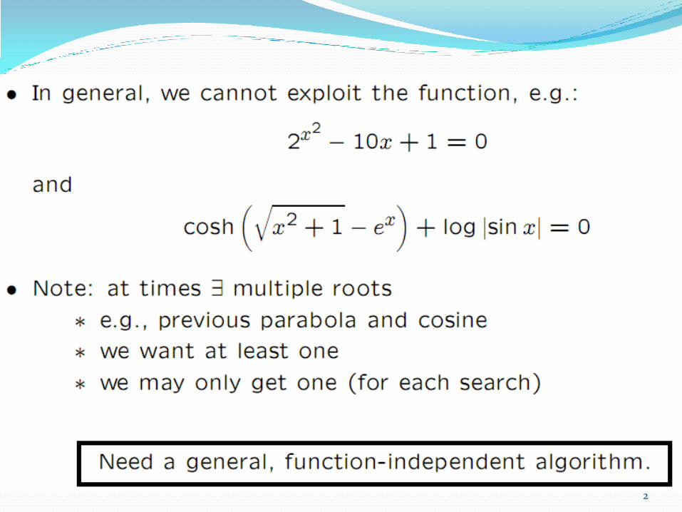
The root of a function f(x) (f:R → R) is simply some value r for which the function is zero, that is, f(r) = 0. This topic is broken into two major sub-problems: Finding the root of a real-valued function of a single variable, and 1. Finding the root of a vector-valued function of a many variables. 2. There are five techniques which may be used to find the root of a univariate (single variable) function: • Bisection method • False-position method • Newton's method • Secant method • Fixed point iteration Given a vector-valued multivariate function f(x) (f:Rn → Rn), we will focus on a generalization of Newton's method to find a vector of values r such that each of the functions is zero, that is, f(r) = 0.

Root Finding

3

Intermediate Value Theorem (IVT) Given a continuous real-valued function f(x) defined on an interval [a, b], then if y is a point between the values of f(a) and f(b), then there exists a point r such that y = f(r). As an example, consider the function f(x) = sin(x) defined on [1, 6]. The function is continuous on this interval, and the point 0.5 lies between the values of sin(1) ] 0.841 and sin(6) e -0.279. Thus, there is at least one point r (there may be more) on the interval [1, 6] such that sin(r) = 0.5. In this case, r 2.61799. This is shown in Figure 1.

Theory

4

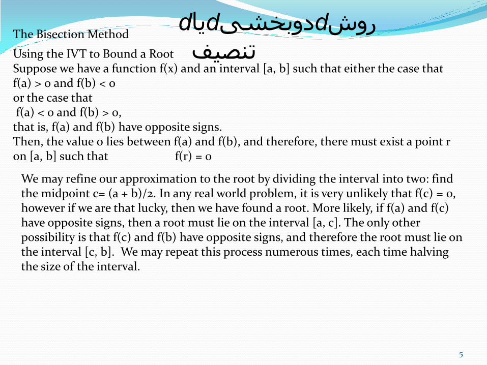
Using the IVT to Bound a Root Suppose we have a function f(x) and an interval [a, b] such that either the case that f(a) > 0 and f(b) < 0 or the case that f(a) < 0 and f(b) > 0, that is, f(a) and f(b) have opposite signs. Then, the value 0 lies between f(a) and f(b), and therefore, there must exist a point r on [a, b] such that f(r) = 0

The Bisection Method

We may refine our approximation to the root by dividing the interval into two: find the midpoint c= (a + b)/2. In any real world problem, it is very unlikely that f(c) = 0, however if we are that lucky, then we have found a root. More likely, if f(a) and f(c) have opposite signs, then a root must lie on the interval [a, c]. The only other possibility is that f(c) and f(b) have opposite signs, and therefore the root must lie on the interval [c, b]. We may repeat this process numerous times, each time halving the size of the interval.

یا دوبخشی روش

تنصیف

5

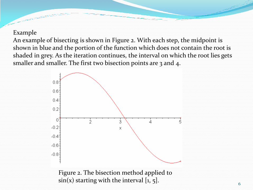
Example An example of bisecting is shown in Figure 2. With each step, the midpoint is shown in blue and the portion of the function which does not contain the root is shaded in grey. As the iteration continues, the interval on which the root lies gets smaller and smaller. The first two bisection points are 3 and 4.

Figure 2. The bisection method applied to sin(x) starting with the interval [1, 5].

6

7

HOWTO

Problem Given a function of one variable, f(x), find a value r (called a root) such that f(r) = 0.

Assumptions We will assume that the function f(x) is continuous.

Tools We will use sampling, bracketing, and iteration.

Initial Requirements We have an initial bound [a, b] on the root, that is, f(a) and (b) have opposite signs.

Iteration Process Given the interval [a, b], define c = (a + b)/2. Then

if f(c) = 0 (unlikely in practice), then halt, as we have found a root,

if f(c) and f(a) have opposite signs, then a root must lie on [a, c], so assign b = c,

else f(c) and f(b) must have opposite signs, and thus a root must lie on [c, b], so assign a = c

8

Halting Conditions There are three conditions which may cause the iteration process to halt:

As indicated, if f(c) = 0.

1.We halt if both of the following conditions are met:

The width of the interval (after the assignment) is sufficiently small, that is b - a < εstep,

And The function evaluated at one of the end point |f(a)| or |f(b)| < εabs.

2. If we have iterated some maximum number of times, say N, and have not met

Condition 1, we halt and indicate that a solution was not found.

3. If we halt due to Condition 1, we state that c is our approximation to the root. If we

halt according to Condition 2, we choose either a or b, depending on whether |f(a)| <

|f(b)| or |f(a)| > |f(b)|,

respectively.

If we halt due to Condition 3, then we indicate that a solution may not exist (the function

may be

discontinuous).

9

10

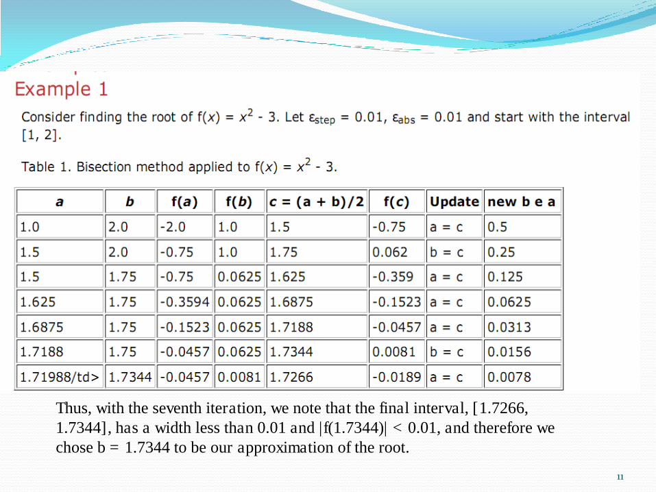
Thus, with the seventh iteration, we note that the final interval, [1.7266,

1.7344], has a width less than 0.01 and |f(1.7344)| < 0.01, and therefore we

chose b = 1.7344 to be our approximation of the root.

11

Thus, after the 11th iteration, we note that the final interval, [3.2963, 3.2968] has a width less

than 0.001 and |f(3.2968)| < 0.001 and therefore we chose b = 3.2968 to be our approximation

of the root. 12

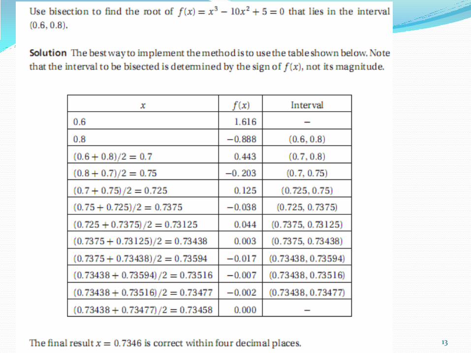
13

14

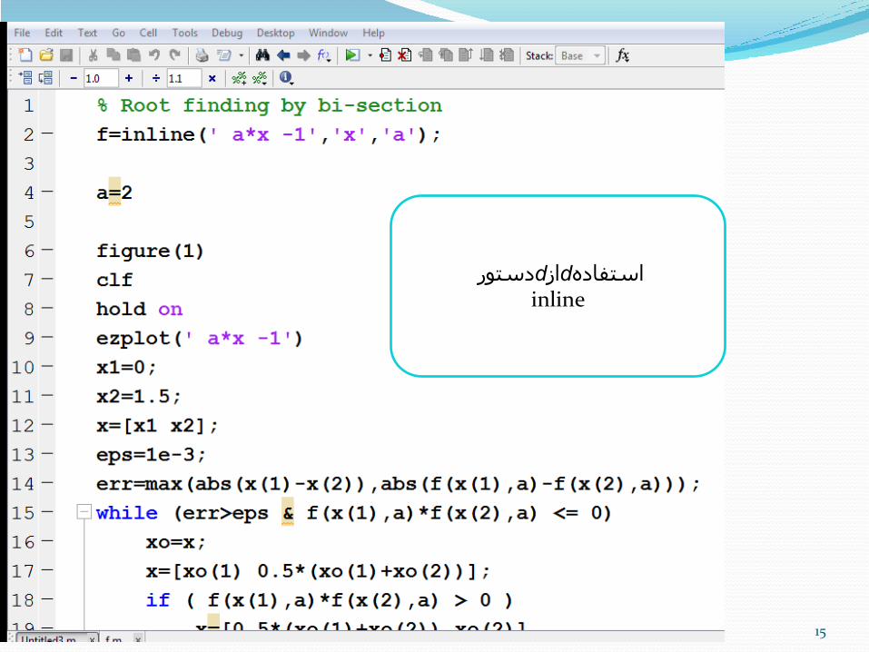
15

دستور از استفادهinline

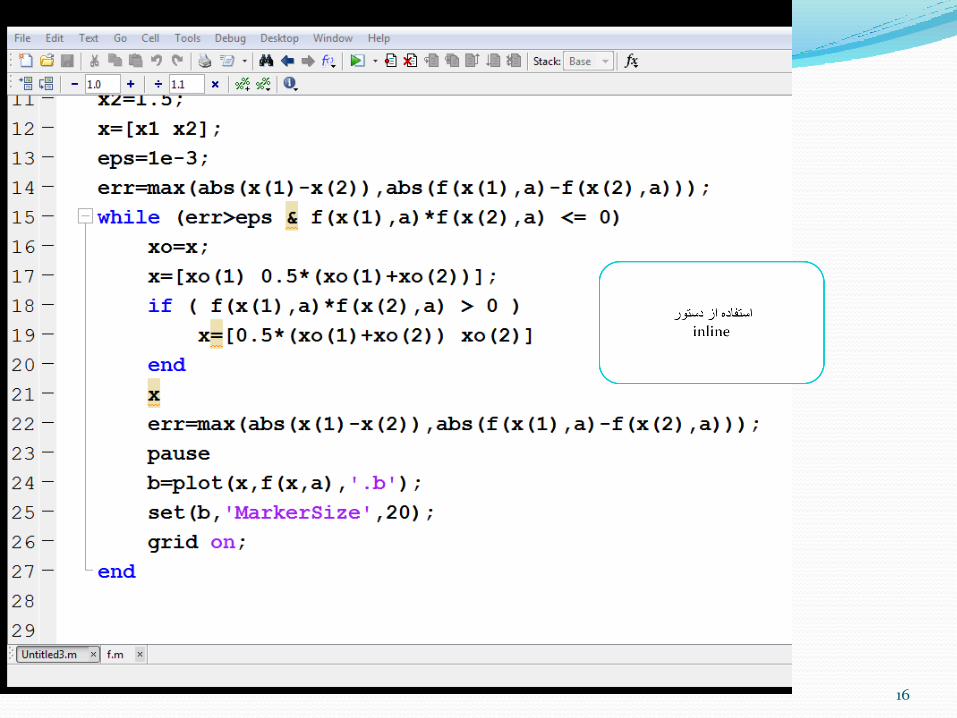
16

17

-ام یک درون تابع تعریف

فایل

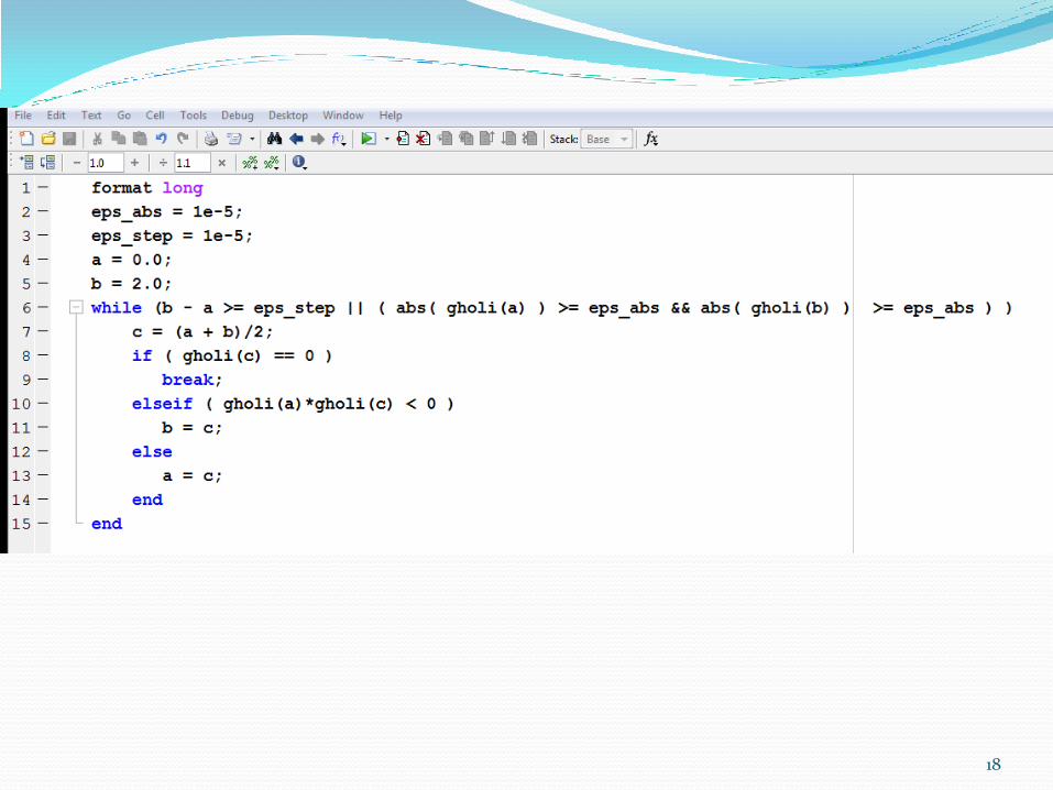
18

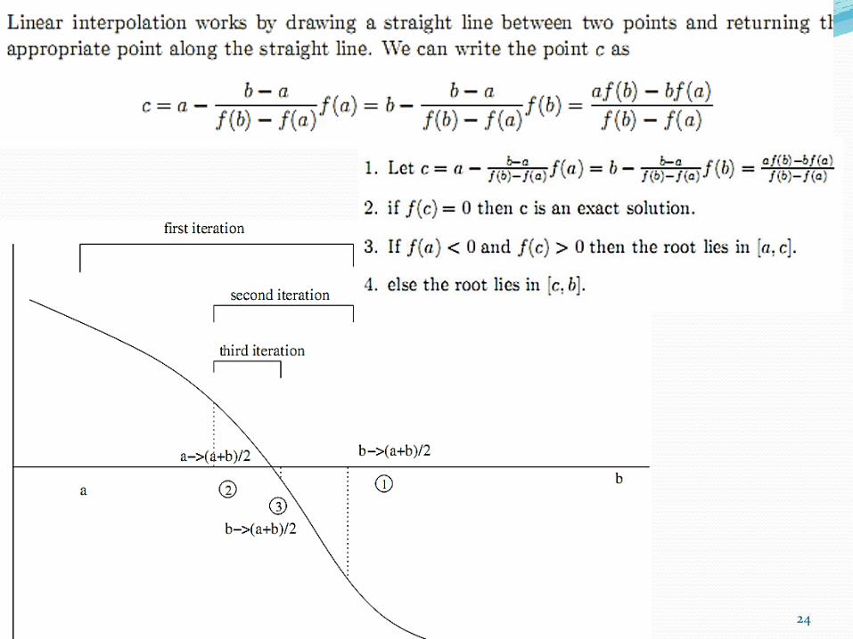
Introduction The false-position method is a modification on the bisection method: if it is known that the root lies on [a, b], then it is reasonable that we can approximate the function on the interval by interpolating the points (a, f(a)) and (b, f(b)). In that case, why not use the root of this linear interpolation as our next approximation to the root?

The False-Position Method نابجایی روش

19

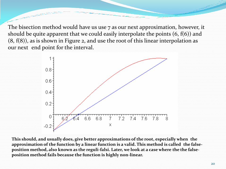
The bisection method would have us use 7 as our next approximation, however, it should be quite apparent that we could easily interpolate the points (6, f(6)) and (8, f(8)), as is shown in Figure 2, and use the root of this linear interpolation as our next end point for the interval.

This should, and usually does, give better approximations of the root, especially when the approximation of the function by a linear function is a valid. This method is called the false-position method, also known as the reguli-falsi. Later, we look at a case where the the false-position method fails because the function is highly non-linear.

20

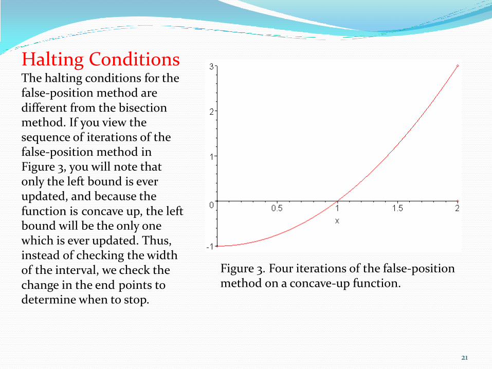
Halting Conditions The halting conditions for the false-position method are different from the bisection method. If you view the sequence of iterations of the false-position method in Figure 3, you will note that only the left bound is ever updated, and because the function is concave up, the left bound will be the only one which is ever updated. Thus, instead of checking the width of the interval, we check the change in the end points to determine when to stop.

Figure 3. Four iterations of the false-position method on a concave-up function.

21

If we cannot assume that a function may be interpolated by a linear function, then applying the false-position method can result in worse results than the bisection method. For example, Figure 4 shows a function where the false-position method is significantly slower than the bisection method. Such a situation can be recognized and compensated for by falling back on the bisection method for two or three iterations and then resuming with the false-position method.

The Effect of Non-linear Functions

Figure 4. Twenty iterations of the false-position method on a highly-nonlinear function

22

HOWTO Problem Given a function of one variable, f(x), find a value r (called a root) such that f(r) = 0.

Assumptions We will assume that the function f(x) is continuous.

Tools We will use sampling, bracketing, and iteration.

Initial Requirements We have an initial bound [a, b] on the root, that is, f(a) and (b) have opposite signs. Set the variable step = l.

Iteration Process Given the interval [a, b], define c = (a f(b) b f(a))/(f(b) / f( a)). Then if f(c) = 0 (unlikely in practice), then halt, as we have found a root, if f(c) and f(a) have opposite signs, then a root must lie on [a, c], so assign step = b - c and assign b = c, else f(c) and f(b) must have opposite signs, and thus a root must lie on [c, b], so assign step = c - a and assign a = c.

23

24

25

26

27

28

29

30