BIS Working Papers · Keywords: housing markets, residential investment , house prices, business cycle s, construction, interest rates, recession forecasts : ... demographic factors

BIS Working Papers No 726

Residential investment and economic activity: evidence from the past five decades by Emanuel Kohlscheen, Aaron Mehrotra and Dubravko Mihaljek

Monetary and Economic Department

June 2018

JEL classification: E22, E32, E37, E43, E52, F44

Keywords: housing markets, residential investment, house prices, business cycles, construction, interest rates, recession forecasts

BIS Working Papers are written by members of the Monetary and Economic Department of the Bank for International Settlements, and from time to time by other economists, and are published by the Bank. The papers are on subjects of topical interest and are technical in character. The views expressed in them are those of their authors and not necessarily the views of the BIS.

This publication is available on the BIS website (www.bis.org).

© Bank for International Settlements 2018. All rights reserved. Brief excerpts may be reproduced or translated provided the source is stated.

ISSN 1020-0959 (print) ISSN 1682-7678 (online)

http://www.bis.org/

1

Residential investment and economic activity: evidence from the past five decades1

Emanuel Kohlscheen, Aaron Mehrotra and Dubravko Mihaljek

Abstract

We analyse the evolution and main drivers of residential investment, using a panel with quarterly data for 15 advanced economies since the 1970s. Residential investment is a notably volatile component of real GDP in all countries in the sample. We find real house price growth, net migration inflows and the size of the existing housing stock to be significant drivers of residential investment across various model specifications. We also detect important asymmetries: interest rate increases affect residential investment more than interest rate cuts, and interest rate changes have larger effects on residential investment when its share in overall GDP is rising. Finally, we show that adding information on residential investment significantly improves the performance of standard recession prediction models.

JEL classification: E22, E32, E37, E43, E52, F44

Keywords: housing markets, residential investment, house prices, business cycles, construction, interest rates, recession forecasts

1 The views expressed in this paper are those of the authors and do not necessarily reflect those of the Bank for International Settlements. Taejin Park provided excellent research assistance. We thank Yavuz Arslan, Ryan Banerjee, Claudio Borio, Stijn Claessens, Fabrizio Coricelli, Boris Hofmann, Enisse Kharroubi, Marco Lombardi, Hyun Song Shin, Christian Upper, Martin Wagner, Fabrizio Zampolli, participants of the European Investment Bank’s workshop “European Network for Research on Investment”, and seminar participants at the BIS for helpful comments and discussions.

E-mail addresses: [email protected]; [email protected] and [email protected]

mailto:[email protected]

mailto:[email protected]

2

1. Introduction

Most research on residential investment focuses on the role of booms and busts in house prices and housing credit for macroeconomic and financial sector outcomes. For example, Jordà et al (2016) documented how mortgage credit booms in advanced economies since the Second World War were increasingly associated with deeper recessions and slower recoveries. The co-movement of property prices and credit also features prominently in modelling financial cycles, whose peaks are closely associated with financial crises (Borio (2014), Claessens et al (2012)).

Research on the macroeconomic implications of residential investment in terms of volumes – housing output produced for the market – is much scarcer. This is surprising given that residential investment is one of the most volatile components of GDP, and given the recent experience with housing booms and busts in countries such as the United States, Ireland and Spain, or in the Nordic countries in the 1990s. Similarly, there is little cross-country analysis of the drivers of residential investment, including interest rates and their potentially asymmetric effects over the cycle. For policymakers this is an important issue: in an economy burdened by oversupply of housing after a housing boom, lower interest rates may do little to kick-start residential investment and economic activity.

This paper intends to fill part of this gap. One contribution we make is to examine the proximate drivers of residential investment in a cross-country rather than single-country context over the past half century. This helps us uncover common financial, demographic and real economy factors related to both demand and supply, rather than idiosyncratic, country-specific factors. Another is to formally study the behaviour of residential investment across the business cycle. In particular, we examine the leading indicator properties of residential investment in a simple recession prediction model.

The paper highlights three main findings. First, we show that the main determinants of residential investment in advanced economies are real house prices, nominal interest rates, demographic factors, and the state of housing supply. House prices seem to play a prominent role by affecting the incentives to invest in housing construction, ie the numerator in Tobin’s q for housing.

Second, we find that the effects of interest rates on residential investment are twice as large during housing booms than during the busts, and are clearly stronger when interest rates are rising than when they are falling.

Third, drops in residential investment consistently lead economic downturns in the 99 recessions identified in our sample. This signalling property arises despite the small overall share of residential investment in GDP – around 6% on average over the past five decades. Prior to an economic downturn, house prices, construction activity and construction employment all decline. We show that information on declines in residential investment improves the performance of standard recession forecasting models that also feature the slope of the yield curve.

Our work is related to several strands of literature. One covers studies of residential investment over the business cycle, in particular its recession prediction properties (Leamer (2007) and (2015); IMF (2008)). For instance, Leamer (2015) showed how nine out of eleven recessions in the United States after the Second World War were preceded by large declines in residential investment. We confirm these properties in a much broader, cross-country setting, and highlight the economic mechanisms that may lie behind them. The relevance of housing dynamics for economic activity is consistent with the models of Iacoviello (2005) and Iacoviello and Neri (2010), in which housing wealth affects spending

3

through changes in collateral values and hence borrowing constraints. Our analysis with recession prediction models is also related to papers such as Estrella and Hardouvelis (1991) and Rudebush and Williams (2009)).

Another strand is studies of the determinants of residential investment, which have focused mainly on the United States. Our finding that residential investment in a broad range of advanced economies responds first and foremost to house price developments is in line with theoretical model predictions and empirical studies for individual countries, such as for instance Topel and Rosen (1988), Tsoukis and Westaway (1994), Davis and Heathcote (2005) and Glaeser et al (2008). Our study also relates to a number of papers that highlight the interest rate sensitivity of residential investment (eg McCarthy and Peach (2002), Erceg and Levin (2006), Jarocinski and Smets (2008), Aspachs-Bracons and Rabanal (2011), Dokko et al (2011), Calza et al (2013)). One implication of this finding is that tighter monetary policy could have curtailed the magnitude of the pre-crisis housing boom in the United States (Taylor (2007), Sutton et al (2017)).

A third strand of the literature we build on is studies of asymmetric effects of interest rate changes on aggregate output (eg Angrist et al (2013), Vavra (2014), Tenreyro and Thwaites (2016)). We find that the effects of interest rates on residential investment are stronger during housing booms and when interest rates are rising. We suggest that one source for this asymmetry could be downward house price rigidity, which forces adjustments to occur via quantities, as already noted by Poterba (1984). Another is investment adjustment costs, which constrain increases more than decreases in activity. More generally, our results corroborate the notion that booms that lead to a temporary oversupply of housing tend to be followed by periods of weak or unresponsive residential investment (Rognlie et al (2018)). One implication is that prolonged construction booms fuelled by expansionary monetary policy could over time weaken the responsiveness of residential investment to monetary policy.

The paper is structured as follows. Section 2 lays out the data and describes some stylised facts on residential investment. Section 3 describes the empirical approach. Section 4 discusses the determinants of residential investment. Section 5 presents results from a formal recession prediction model that incorporates residential investment. Results of various robustness tests are shown in Section 6. Section 7 concludes.

2. Data and stylised facts

Our analysis on residential investment is based on a longer data sample than previous cross-country studies on the topic (eg Calza et al (2013); IMF (2008)). The data for residential investment are from the OECD’s Economic Outlook Database, complemented with information from national statistical authorities. For Germany, data for West Germany from the German Federal Statistical Office are used prior to 1991. Residential investment data for Switzerland are based on gross private domestic investment in construction provided by the State Secretariat for Economic Affairs (SECO).

In order to compute the size of the existing housing stock, we use the estimates on initial housing stocks by Piketty and Zucman (2014). We then compute the stocks in subsequent periods assuming a 1½% annual depreciation.2

2 In a robustness check we also estimated the model using a 2% depreciation rate.

4

For real house prices, we use residential property prices published by the BIS and deflated by the national consumer price index. For most countries in the sample, these series are based on transactions data. They also feature a quality adjustment, either based on size only or using a more sophisticated method, such as a hedonic regression (see Scatigna et al (2014)).

Our sample runs from 1970 Q1 to 2017 Q2. We include 15 advanced economies: Australia, Canada, France, Germany, Italy, Japan, the Netherlands, New Zealand, Norway, Korea, Spain, Sweden, Switzerland, the United Kingdom and the United States.

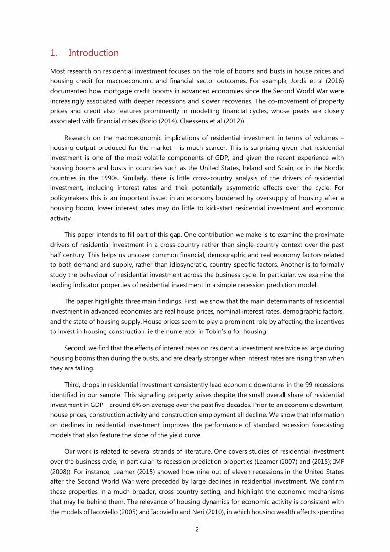
Residential investment generally accounts for a small share of GDP. Over the whole sample, it averaged 5.9% of GDP, compared with 12.5% for business investment. The share has fallen over time from 7.3% in the first two decades, to 5.8% between 1991 and the Great Financial Crisis (GFC), and then to 4.7% in 2008–16 (Graph 1). Only Canada and Norway – shown on the right-hand side of the graph – have seen an increase in the share of residential investment post-crisis.

Residential investment used to be much higher in the past Per cent of GDP Graph 1

1 Period averages of quarterly data. For Switzerland, annual data. Countries are ordered by the residential investment share in 2008–16.

Sources: OECD, Economic Outlook database; national data; BIS calculations.

Historically, the share of residential investment in GDP was highest during the 1970s and 1980s, especially in Sweden (10%), where construction surged during the “Million Homes Programme” (1965–75), which aimed to overcome urbanisation-induced housing shortages (Emanuelsson (2015)). In the two decades before the GFC, the share of residential investment was highest in Spain (8%), where easy financing conditions that accompanied the introduction of the euro, demographic factors and purchases by other EU residents played a role (eg Garcia-Herrero and Fernandez de Lis (2008)).

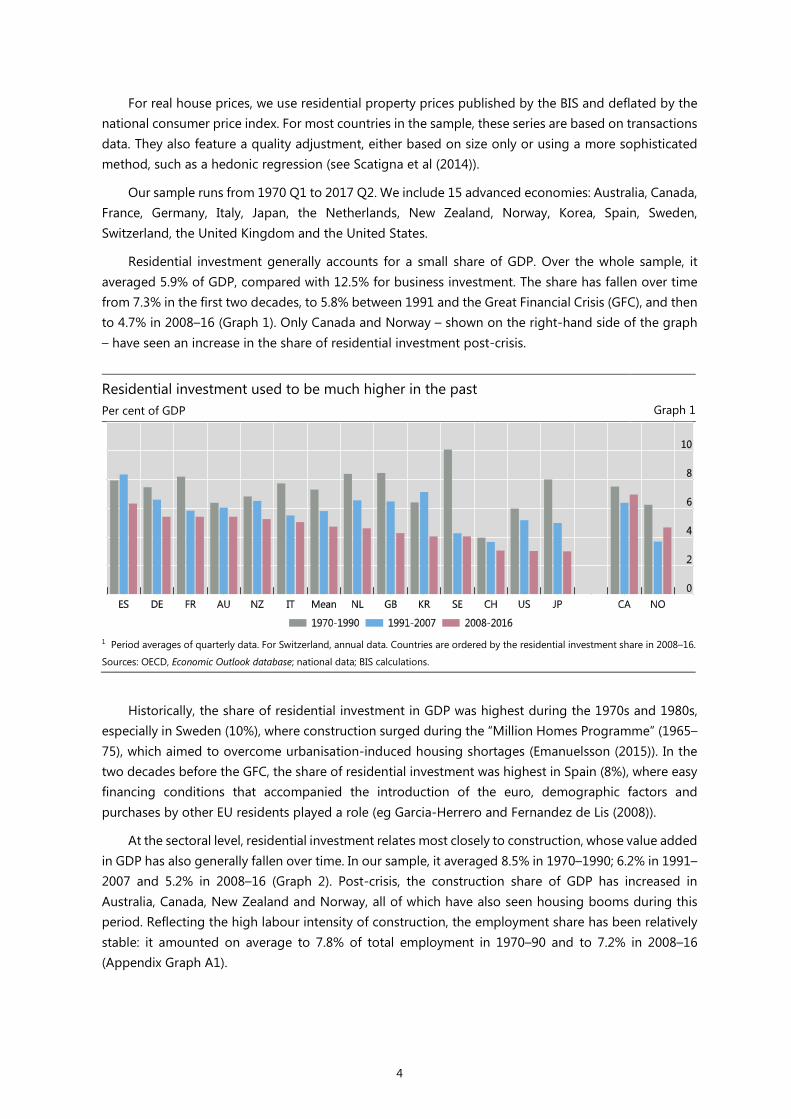
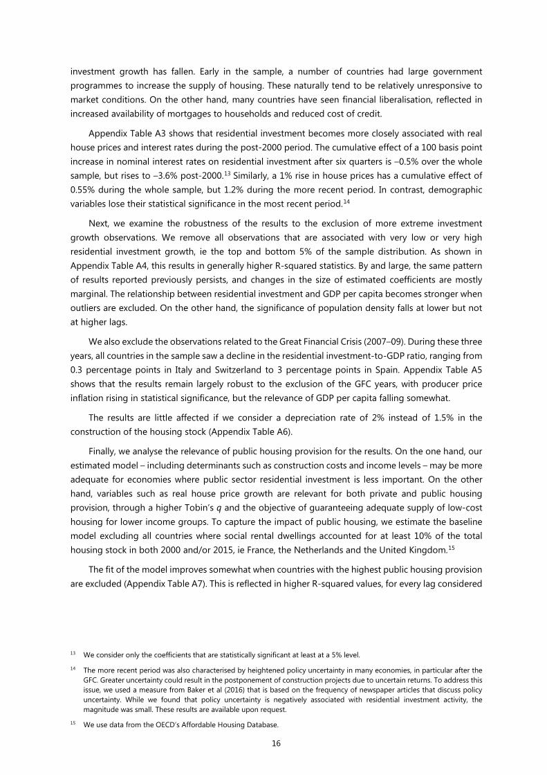
At the sectoral level, residential investment relates most closely to construction, whose value added in GDP has also generally fallen over time. In our sample, it averaged 8.5% in 1970–1990; 6.2% in 1991–2007 and 5.2% in 2008–16 (Graph 2). Post-crisis, the construction share of GDP has increased in Australia, Canada, New Zealand and Norway, all of which have also seen housing booms during this period. Reflecting the high labour intensity of construction, the employment share has been relatively stable: it amounted on average to 7.8% of total employment in 1970–90 and to 7.2% in 2008–16 (Appendix Graph A1).

5

Construction value added has declined over time As per cent of GDP Graph 2

1 Period averages of annual data. For Japan, data are available to 2015; for New Zealand, data are available from 1971 to 2015.

Sources: OECD; Datastream; national data; BIS calculations.

Notwithstanding its generally small share in the overall economy, residential investment is often

the most volatile component of GDP (Graph 3). Volatility arises in part from the large housing stock: even small changes in desired housing stock require relatively large changes in investment. Measured by the standard deviation, volatility of residential investment in our sample is on average about five times that of overall GDP growth. This compares with a ratio of around four-to-one for business investment. Residential investment volatility in our sample has been highest in Korea and the Netherlands, at around 8–9 times that of GDP. Norway is an exception to this pattern, as growth in business investment, which is driven by oil production, is more volatile than that in residential investment. Yet, both series are far more volatile than GDP growth.

Residential and business investment are much more volatile than GDP growth1 Standard deviation of seasonally-adjusted quarterly growth Graph 3

1 Data for 1970–2016. Business investment includes investment in commercial property. For Germany prior to 1991, Italy and Spain, computed as total less housing investment. For Switzerland, construction is used for residential, and equipment and software for business investment.


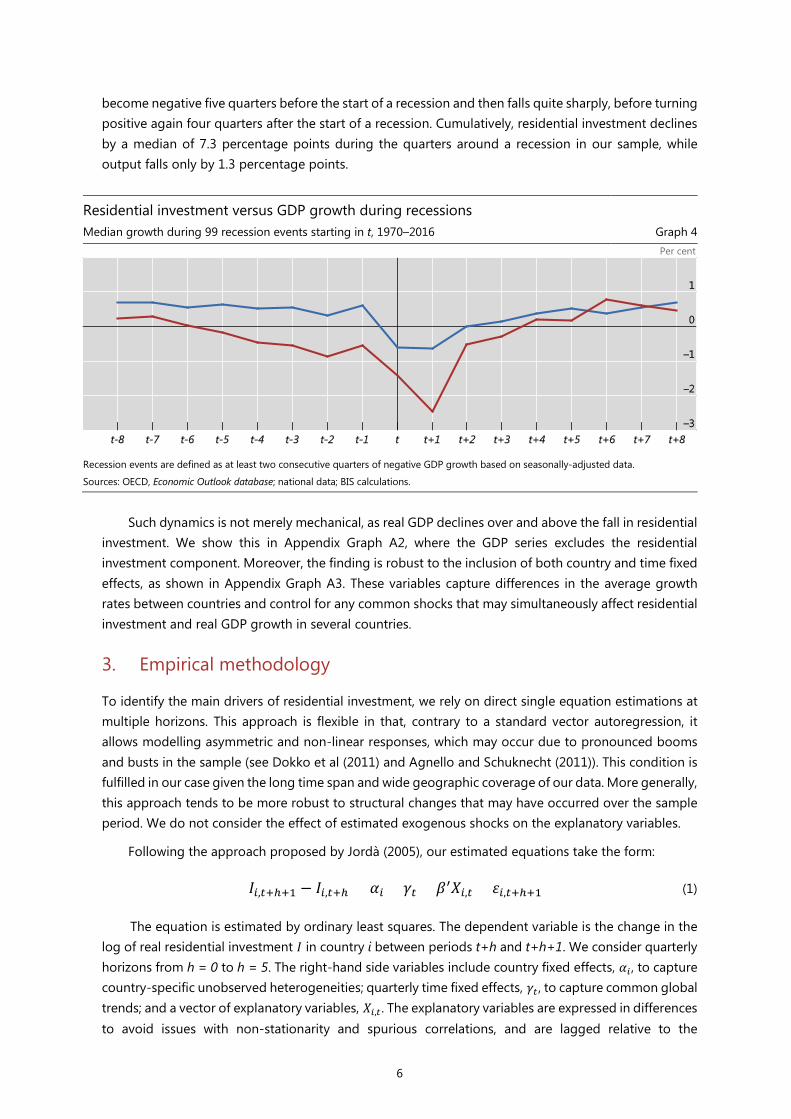
Consistent with high overall volatility, residential investment tends to fall sharply before recessions,

with a notable lead over broader economic activity. Defining recessions conventionally, as a minimum of two consecutive periods of negative quarter-on-quarter GDP growth, Graph 4 shows the median growth rates in real GDP (blue line) and residential investment (red line), before and after the start of a recession (in quarter t). The sample includes 99 recessions. Residential investment growth tends to

6

become negative five quarters before the start of a recession and then falls quite sharply, before turning positive again four quarters after the start of a recession. Cumulatively, residential investment declines by a median of 7.3 percentage points during the quarters around a recession in our sample, while output falls only by 1.3 percentage points.

Residential investment versus GDP growth during recessions Median growth during 99 recession events starting in t, 1970–2016 Graph 4

Per cent

Recession events are defined as at least two consecutive quarters of negative GDP growth based on seasonally-adjusted data.


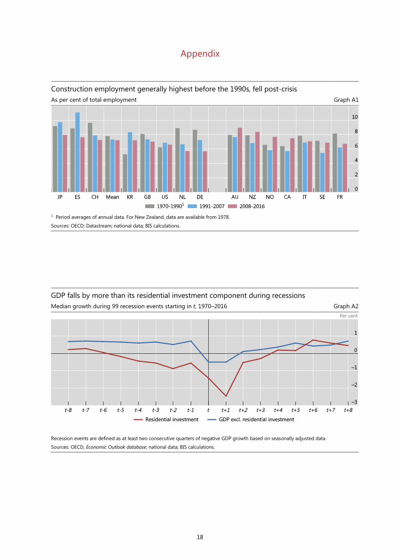
Such dynamics is not merely mechanical, as real GDP declines over and above the fall in residential

investment. We show this in Appendix Graph A2, where the GDP series excludes the residential investment component. Moreover, the finding is robust to the inclusion of both country and time fixed effects, as shown in Appendix Graph A3. These variables capture differences in the average growth rates between countries and control for any common shocks that may simultaneously affect residential investment and real GDP growth in several countries.

3. Empirical methodology

To identify the main drivers of residential investment, we rely on direct single equation estimations at multiple horizons. This approach is flexible in that, contrary to a standard vector autoregression, it allows modelling asymmetric and non-linear responses, which may occur due to pronounced booms and busts in the sample (see Dokko et al (2011) and Agnello and Schuknecht (2011)). This condition is fulfilled in our case given the long time span and wide geographic coverage of our data. More generally, this approach tends to be more robust to structural changes that may have occurred over the sample period. We do not consider the effect of estimated exogenous shocks on the explanatory variables.

Following the approach proposed by Jordà (2005), our estimated equations take the form:

𝐼𝐼𝑖𝑖,𝑡𝑡+ℎ+1 − 𝐼𝐼𝑖𝑖,𝑡𝑡+ℎ = 𝛼𝛼𝑖𝑖 + 𝛾𝛾𝑡𝑡 + 𝛽𝛽′𝑋𝑋𝑖𝑖,𝑡𝑡 + 𝜀𝜀𝑖𝑖,𝑡𝑡+ℎ+1 (1)

The equation is estimated by ordinary least squares. The dependent variable is the change in the log of real residential investment 𝐼𝐼 in country i between periods t+h and t+h+1. We consider quarterly horizons from h = 0 to h = 5. The right-hand side variables include country fixed effects, 𝛼𝛼𝑖𝑖 , to capture country-specific unobserved heterogeneities; quarterly time fixed effects, 𝛾𝛾𝑡𝑡 , to capture common global trends; and a vector of explanatory variables, 𝑋𝑋𝑖𝑖,𝑡𝑡 . The explanatory variables are expressed in differences to avoid issues with non-stationarity and spurious correlations, and are lagged relative to the

7

dependent variable to minimise reverse causality concerns. At the same time, we acknowledge that simultaneity issues cannot be fully eliminated in the framework.

The vector of explanatory variables 𝑋𝑋𝑖𝑖,𝑡𝑡 includes various components of Tobin’s q for residential investment that capture the incentives to invest in housing. Tobin’s q for housing compares the market price of a new home in the numerator to various costs of building a new home in the denominator. As in Tsoukis and Westaway (1994), we include the components for Tobin’s q in the regression individually, as there is considerable uncertainty regarding the measurement and weights of such components in any constructed measure of q.

Our house price series are computed as residential property prices deflated by the consumer price index. Arguably, time-to-build considerations, as in Kydland and Prescott (1982), imply that it is the expected house prices that matter for investment decisions. Given the lack of published house price forecasts and the well documented persistence in house price trends, we proxy the expected changes by actual house price changes in the current period. Sutton et al (2017) argue that forecastable upward moves in house prices tend to persist because of the large search and transaction costs associated with house purchases. Similarly, Glaeser and Gyourko (2007) regard the serial correlation of house price changes as one key stylised fact of the housing market. This implies that the most recent changes contain information on the likely future trend in prices.

Given the inclusion of various lags of real house price growth in the regression, our approach captures investment adjustment costs, whereby changes in real house prices affect residential construction only slowly over time. House prices also reflect any additional effects of residential investment that are not well captured by other explanatory variables, and for which little comparable cross-country data are available. These include housing quality adjustments, the effects of restrictive regulations on housing supply, or, in some countries, the effects of foreign demand on residential investment. We also note that house prices matter for the incentives to construct new housing and undertake home improvements, both of which are included in the residential investment series.

Regarding components that enter the denominator of Tobin’s q, we include inflation measured by the producer price index (PPI) as a proxy for construction costs. Higher costs of raw materials, including energy, push up construction costs and negatively affect investment in new or the expansion of existing residential units. Another cost variable we include is the short-term interest rate, which affects both housing supply (through property developers’ funding costs) and housing demand (through debt servicing costs). Interest rates also affect investment indirectly, through discount rates used in property valuations (the numerator of q). We use a short-term money market rate, in line with Mishkin’s (2007) argument that builders construct houses relatively quickly, making short-term rates relevant for the financing of house construction. The interest rate is nominal, as in Topel and Rosen (1988) and as money illusion phenomena may be important (Tsoukis and Westaway (1994); Sutton et al (2017)). With real interest rates we also generally obtain the expected negative signs but with lower statistical and economic significance.

Among demand side variables, we include income levels (GDP per capita), population density (people per square km of land area), and net migration rates (net migrants per 1,000 population). Higher income and greater inward migration are expected to boost residential investment. Higher migration rates can also boost housing supply by increasing the number of construction workers.3 The

3 Corder (2008) argued that labour shortages in the UK’s construction sector eased in the 2000s when migrant workers entered the sector.

8

sign for the population density variable is ambiguous a priori: higher population density can constrain additional construction activity, but may also increase the incentive for developers to build more high-rise apartment buildings and fewer single family houses.

Finally, we include the stock of housing in relation to GDP. Larger existing stocks relative to the size of the economy should reduce the incentives to pursue additional residential investment.

4. Estimation results

4.1 Baseline specifications The baseline estimates in Table 1, with over 2,700 country-quarter observations, show that most of our explanatory variables have an economically and statistically significant impact on residential investment over multiple horizons. This suggests that a sufficiently flexible modelling approach that considers various different lags is indeed appropriate. Furthermore, all coefficients have the expected sign whenever they are statistically significant at conventional levels.

Several findings are worth highlighting. First, higher real house prices are positively correlated with

residential investment. A 1% increase in real house prices is associated with a 0.35% rise in residential investment already after one quarter, and 0.55% after two quarters.4 Changes in interest rates are

4 In theory, house price changes would be irrelevant for residential investment only if they were perceived to be entirely temporary. In practice, they are likely to carry new information about the trend and hence about rising or falling returns in the housing sector.

Determinants of residential investment growth: 1970–2017 Table 1Dependent variable: Residential investment growth (real, log differences)

(I) (II) (III) (IV) (V) (VI)t+1 t+2 t+3 t+4 t+5 t+6

PPI inflation –0.070* –0.05 –0.051* –0.041 –0.021 0.009 t-stat 1.84 1.55 1.71 1.02 0.59 0.33Real house price growth 0.352*** 0.199*** 0.059 0.059 –0.012 –0.014 t-stat 6.29 2.84 0.71 1.09 0.17 0.28Interest rate change –0.016 –0.148 –0.203** –0.205** –0.111* 0.072 t-stat 0.16 1.38 2.03 2.33 1.80 0.72Population density change 0.011 0.023** 0.021*** 0.020** 0.029*** 0.022*** t-stat 1.19 2.36 2.89 2.53 3.34 2.98Net migration rate change 0.023*** 0.026*** 0.029*** 0.030*** 0.028*** 0.033*** t-stat 2.89 3.28 3.26 3.36 3.47 2.78Housing stock/GDP –0.005** –0.006*** –0.007** –0.008** –0.009*** –0.007** t-stat 2.43 3.14 2.39 2.56 2.99 2.34GDP per capita change 0.154 0.355** 0.231 0.132 0.271 0.156 t-stat 0.59 2.04 1.56 1.49 1.59 1.30Country fixed effects yes yes yes yes yes yesTime fixed effects yes yes yes yes yes yesObservations 2,740 2,740 2,739 2,738 2,723 2,708R2 0.148 0.140 0.132 0.130 0.128 0.127F statistic 10.94*** 9.83*** 11.27*** 7.77*** 9.83*** 5.66***RMSE 0.052 0.052 0.052 0.052 0.052 0.052Note: Time span is from 1970 Q1 to 2017 Q2. All right-hand side variables are at period t . Reported t -statistics below coefficients arebased on robust standard errors clustered by country. ***/**/* denote statistical significance at 1, 5 and 10%, respectively. Countriescovered are AU, CA, FR, DE, IT, JP, KR, NL, NZ, NO, ES, SE, CH, GB and US.

Growth in quarter t+h

9

negatively related to residential investment, with a lag. An increase in nominal interest rates by 100 basis points is associated with a 0.20% fall in residential investment after three quarters, and 0.52% after five quarters (if one considers coefficients that are at least significant at a 10% level).5 Comparing normalised estimates instead (not shown), the relationship between residential investment and a one standard deviation change in real house prices is roughly four times as large, in absolute terms, as that of one standard deviation change in interest rates.

Second, demographic factors matter. A higher rate of net migration is associated with greater residential investment. Similarly, an increase in population density is positively correlated with residential investment.6

Third, a larger existing housing stock acts as a break on new residential investment. As a corollary, countries with smaller housing stocks have seen faster growth in residential investment, a finding that is also consistent with higher investment ratios observed in the earlier part of the sample (Graph 1).

Fourth, the coefficients on both GDP per capita and PPI inflation have the expected signs. A 1% increase in income per capita is associated with a rise in residential investment by 0.36% after two quarters. In contrast, a higher rate of PPI inflation, used as a proxy for construction cost growth, is negatively related to residential investment. However, the coefficients in the latter case are only weakly statistically significant.

4.2 Examining asymmetries

Next we identify cyclical phases of residential investment in order to examine whether the effect of interest rates on residential investment is asymmetric across the cycle. We define residential investment upswings as periods when the quarterly change in the residential investment-to-GDP ratio is above the 75th percentile of the distribution (for each country) for at least one year. Thus, upswings are associated with a rapid increase in the share of residential investment in the economy. Similarly, residential investment downswings are defined as periods when the quarterly change in the residential investment-to-GDP ratio is below the 25th percentile of the distribution in each country. During such periods, the share of residential investment in the overall economy falls.

To prevent temporary volatility in residential investment from affecting the identified phases, the cycles are computed using the four-quarter moving averages of residential investment-to-GDP. Short up/downswings lasting less than four quarters are not considered, in order to have sufficient persistence in cyclical phases. Moreover, any gaps of less than four quarters between two identical phases (downswing or upswing) were eliminated, thus combining the two phases into a single one. The resulting 76 cyclical upswings and 65 downswings are shown in Graphs 5 and 6.

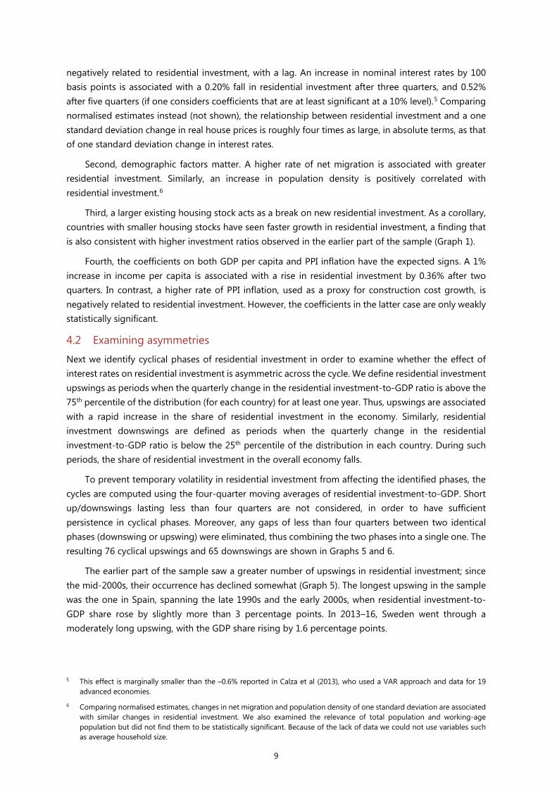
The earlier part of the sample saw a greater number of upswings in residential investment; since the mid-2000s, their occurrence has declined somewhat (Graph 5). The longest upswing in the sample was the one in Spain, spanning the late 1990s and the early 2000s, when residential investment-to-GDP share rose by slightly more than 3 percentage points. In 2013–16, Sweden went through a moderately long upswing, with the GDP share rising by 1.6 percentage points.

5 This effect is marginally smaller than the –0.6% reported in Calza et al (2013), who used a VAR approach and data for 19 advanced economies.

6 Comparing normalised estimates, changes in net migration and population density of one standard deviation are associated with similar changes in residential investment. We also examined the relevance of total population and working-age population but did not find them to be statistically significant. Because of the lack of data we could not use variables such as average household size.

10

Timeline of upswings in residential investment, 1970–2016 1 Graph 5

1 Defined as quarterly growth (in percentage points) above the 75th percentile within each country, based on four-quarter moving averages of residential investment as share of GDP. Short upswings lasting less than four quarters were dropped, and short gaps (less than four quarters) between two upswings) were connected. For Switzerland, construction is used for residential investment.


At the opposite phase of the cycle, many countries saw downswings around the time of the Great

Financial Crisis (Graph 6). Spain experienced a long investment slump during 2007–14, when the residential investment-to-GDP ratio fell by 5.5 percentage points. In the United States, the ratio declined by 3 percentage points in the aftermath of the GFC. In Norway, it fell by a similar amount in the late 1980s and the early 1990s.

Next, we use the identified cyclical phases as zero-one dummy variables interacted with interest rates. We find that a change in interest rates by 100 basis points is associated with a decline in residential investment by 0.8% after four quarters during residential investment upswings (Table 2), and with roughly half that during normal times. 7 Similarly, when we interact rate changes with downswings, we obtain that effects are weaker during these. 8 This evidence is in line with findings for aggregate output by Tenreyro and Thwaites (2016), among others.

One explanation for such dynamics is that borrowers become more sensitive to higher interest rates when residential investment is expanding rapidly. Both property developers and buyers may be incurring higher levels of debt, and if the upturn coincides with a financial boom, marginal borrowers

7 These results use coefficient estimates that are at least statistically significant at a 10% level.

8 These results are not shown here, but are available upon request.

11

may benefit from greater availability of credit. We find some support for this narrative, as real total credit growth is more than twice higher during residential investment upturns than downturns (median growth rates of 1.5% and 0.6%, respectively).

Timeline of downswings in residential investment, 1970–2016 1 Graph 6

1 Defined as quarterly growth (in percentage points) below the 25th percentile within each country, based on four-quarter moving averages of residential investment as share of GDP. Short downswings lasting less than four quarters were dropped, and short gaps (less than four quarters) between two downswings were connected. For Switzerland, construction is used for residential investment.


Does the relationship between interest rates and residential investment differ for interest rate increases and decreases? Previous research has highlighted the asymmetric effects of monetary contractions and expansions on economic activity, with interest rate hikes generally having stronger effects than interest rate cuts (eg Angrist et al (2013)). Table 3 concurs with that evidence, as interest rate increases are found to be associated with lower residential investment, over multiple horizons, with economically and statistically significant coefficients. In contrast, the correlation of residential investment with interest rate declines is not statistically significant at any horizon. The result is not driven by the Great Financial Crisis and its aftermath – additional estimates (not shown) indicate that similar dynamics prevailed from 1970 to 2006.

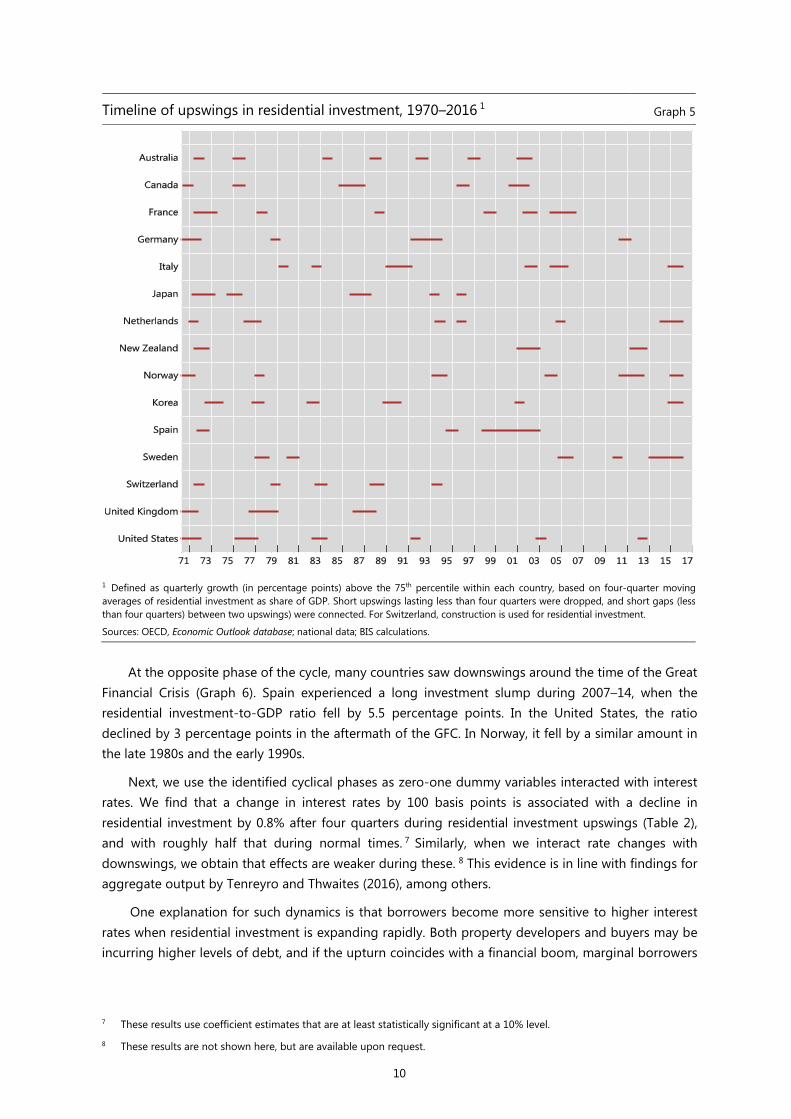
Why would interest rate increases have greater effects on residential investment volumes than interest rate decreases? One reason could be downward rigidity in real house prices. Sellers may be unwilling to let prices fall sufficiently to generate expectations of new price increases. Graph 7 supports this conjecture, showing that house prices rose much more strongly (1.5% quarter-on-quarter) during median residential investment upswings than they fell during median downswings (–0.6%).

12

The asymmetry between upswings and downswings is also pronounced, but in the opposite

direction, for changes in construction value added in total GDP. During a median upswing, the GDP share rose by less than 0.1 percentage point (year-on-year), while it fell by close to 0.3 percentage points during a median downswing. Finally, the fall in the share of employment in the construction

Testing for effects of interest rate changes during upswings Table 2Dependent variable: residential investment growth (real, log differences)


PPI inflation –0.069* –0.050 –0.050 –0.040 –0.020 0.007 t-stat 1.82 1.55 1.68 1.00 0.57 0.26Real house price growth 0.351*** 0.198*** 0.058 0.058 –0.013 –0.012 t-stat 6.27 2.84 0.69 1.10 0.19 0.23Interest rate change 0.008 –0.147 –0.175* –0.187** –0.093 0.035 t-stat 0.08 1.31 1.84 2.20 1.33 0.38Interest rate change * upswing –0.382 –0.015 –0.448** –0.284 –0.287 0.586 t-stat 1.63 0.08 2.31 1.05 1.18 1.04Population density change 0.011 0.023** 0.021*** 0.020*** 0.029*** 0.022*** t-stat 1.22 2.37 3.01 2.59 3.37 2.99Net migration rate change 0.023*** 0.026*** 0.029*** 0.030*** 0.028*** 0.033*** t-stat 2.89 3.28 3.26 3.36 3.47 2.78Housing stock/GDP –0.005** –0.006*** –0.007** –0.008** –0.009*** –0.007** t-stat 2.43 3.14 2.39 2.56 2.99 2.34GDP per capita (log) 0.152 0.355** 0.229 0.131 0.269 0.159 t-stat 0.59 2.04 1.58 1.46 1.58 1.36Country fixed effects yes yes yes yes yes yesTime fixed effects yes yes yes yes yes yesObservations 2,740 2,740 2,739 2,738 2,723 2,708R2 0.149 0.140 0.133 0.130 0.128 0.128F statistic 9.64*** 10.70*** 14.48*** 7.34*** 21.73*** 8.22***RMSE 0.052 0.052 0.052 0.052 0.052 0.052


Note: Time span is from 1970 Q1 to 2017 Q2. All right-hand side variables are at period t . Reported t -statistics below coefficients are based onrobust standard errors clustered by country. ***/**/* denote statistical significance at 1, 5 and 10%, respectively. Countries covered are AU, CA,FR, DE, IT, JP, KR, NL, NZ, NO, ES, SE, CH, GB and US.

Testing for asymmetries: interest rate increases vs decreases Table 3Dependent variable: Residential investment growth (real, log differences)


PPI inflation –0.063* –0.044 –0.047* –0.035 –0.015 0.012 t-stat 1.81 1.47 1.69 0.90 0.45 0.46real house price growth 0.344*** 0.192*** 0.054 0.053 -0.019 -0.018 t-stat 5.94 2.75 0.66 0.98 0.27 0.37Interest rate increase –0.262** –0.350 –0.361*** –0.410*** –0.342** –0.038 t-stat 1.97 1.56 3.80 3.98 2.35 0.21Interest rate decrease 0.255 0.076 –0.030 0.020 0.144 0.195 t-stat 1.28 0.61 0.22 0.15 1.15 1.48Population density change 0.013 0.024** 0.022*** 0.021*** 0.030*** 0.023*** t-stat 1.37 2.48 3.14 2.75 3.45 3.27Net migration rate change 0.023*** 0.026*** 0.029*** 0.030*** 0.027*** 0.033*** t-stat 3.25 3.69 3.63 3.32 3.42 2.76Housing stock/GDP –0.006*** –0.007*** –0.008*** –0.008*** –0.010*** –0.007** t-stat 2.77 3.42 3.80 2.75 3.20 2.44GDP per capita (log) 0.121 0.328* 0.210 0.105 0.240 0.141 t-stat 0.45 1.91 1.39 1.13 1.52 1.17Country fixed effects yes yes yes yes yes yestime fixed effects yes yes yes yes yes yesObservations 2,740 2,740 2,739 2,738 2,723 2,708R2 0.151 0.142 0.133 0.131 0.130 0.127F statistic 35.78*** 10.26*** 35.13*** 8.89*** 11.50*** 5.80***RMSE 0.052 0.052 0.052 0.052 0.052 0.052


Note: Time span is from 1970 Q1 to 2017 Q2. All right hand-side variables are at period t . Reported t -statistics below coefficients arebased on robust standard errors clustered by country. ***/**/* denote statistical significance at 1, 5 and 10%, respectively. Countriescovered are AU, CA, FR, DE, IT, JP, KR, NL, NZ, NO, ES, SE, CH, GB and US.

13

sector was higher in absolute magnitude during a median downswing (–0.17 percentage points; year-on-year), than the increase during an upswing (0.09 percentage points).

These findings corroborate previous evidence that the bulk of the adjustment during downswings occurs through volumes rather than prices (eg Poterba (1984); Leamer (2015)). In contrast, during upswings, investment adjustment costs and labour shortages make it more difficult to increase construction activity than to lower it, as discussed in Corder (2008), resulting in a stronger adjustment through prices than volumes. 9

Interest rate asymmetries could also work through creditworthiness of property developers. Higher interest rates tighten the funding conditions of developers and increase the probability of default, whereas default probabilities are bounded at zero in the case of interest rate declines.

The partly synchronised nature of upswings and downswings in residential investment across countries suggests that there may be an important common global component in residential investment. The quarterly time fixed effects can be regarded as a proxy for “global” residential investment growth, when country fixed effects and various determinants of residential investment have been accounted for. Appendix Graph A4 shows that there are three periods during which time fixed effects turned strongly negative. The first one was in 1974, in the immediate aftermath of the first oil shock, when the Federal Reserve tightened monetary conditions aggressively. The second one was in 1991, when global credit contracted sharply. Finally, the time dummies turned strongly negative between the second half of 2007 and early 2010, during the GFC.

9 We also test the robustness of the findings in Graph 7 to two other definitions of upswings and downswings. First, we construct the 25th and 75th percentiles based on the entire sample distribution (rather than the country-specific distributions) of the change in residential investment-to-GDP ratios. Second, we use the growth in real residential investment, rather than the change in its GDP share, to compute the 25th and 75th percentiles. The asymmetries identified in Graph 7 are robust to these alternative definitions. These results are available upon request.

House prices and construction during residential investment upswings and downswings Graph 7

Real house prices Construction value added3 Construction employment3 Average quarterly growth, per cent Average annual change, % GDP Ave. annual change, % total employment

1 Defined as quarterly growth (in percentage points) above the 75th percentile within each country, based on four-quarter moving averages of residential investment as share of GDP. Short upswings lasting less than four quarters were dropped, and short gaps (less than four quarters) between two upswings were connected. For Switzerland, construction is used for residential investment. 2 Defined as quarterly growth (in percentage points) below the 25th percentile within each country, based on four-quarter moving averages of residential investment as share of GDP. Short downswings lasting less than four quarters were dropped, and short gaps (less than four quarters) between two downswings were connected. 3 When two or more quarters within a calendar year are up- or down-swing quarters, the whole year is considered an up- or down-swing period.


14

Of course the inclusion of time fixed effects stacks the cards against finding significant effects from other explanatory variables. Indeed, if time fixed effects are omitted, the coefficients on other right-hand side variables increase in statistical significance (see Appendix Table A1). Nevertheless, given the higher explanatory power of the models with time fixed effects, together with the possibility that they capture relevant and otherwise omitted global conditions, we include them in our baseline estimations.

5. Evidence from recession prediction models

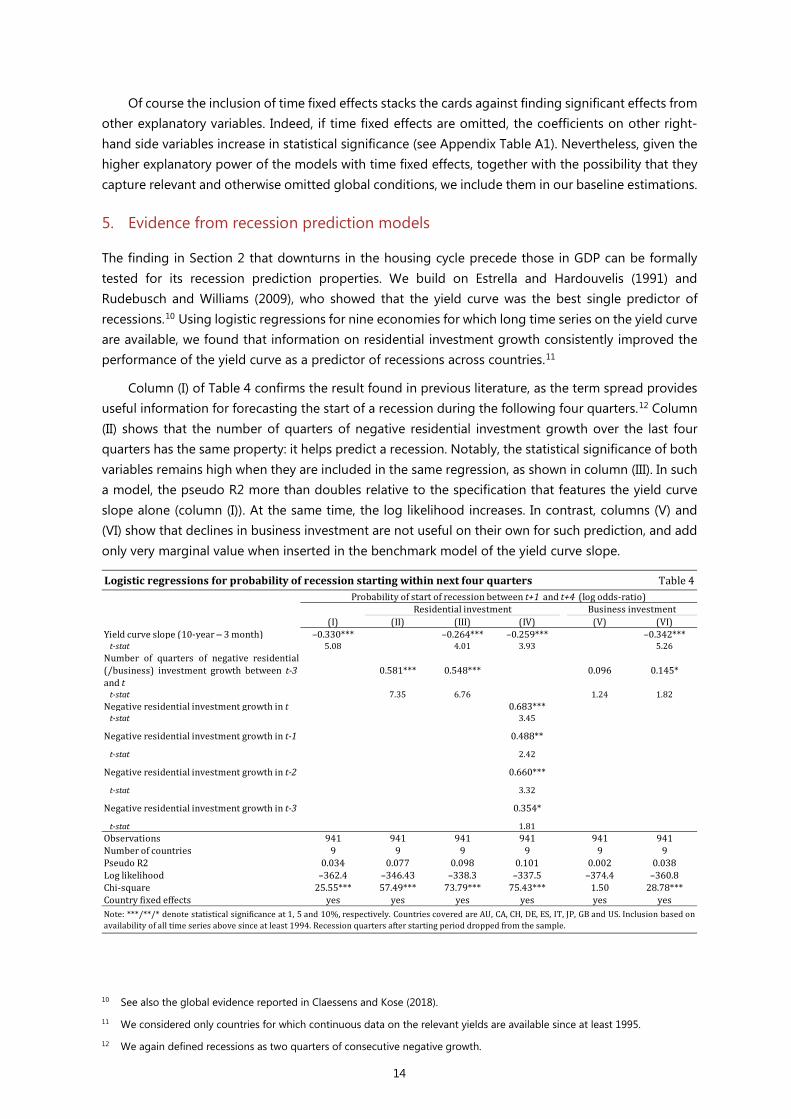
The finding in Section 2 that downturns in the housing cycle precede those in GDP can be formally tested for its recession prediction properties. We build on Estrella and Hardouvelis (1991) and Rudebusch and Williams (2009), who showed that the yield curve was the best single predictor of recessions.10 Using logistic regressions for nine economies for which long time series on the yield curve are available, we found that information on residential investment growth consistently improved the performance of the yield curve as a predictor of recessions across countries.11

Column (I) of Table 4 confirms the result found in previous literature, as the term spread provides useful information for forecasting the start of a recession during the following four quarters.12 Column (II) shows that the number of quarters of negative residential investment growth over the last four quarters has the same property: it helps predict a recession. Notably, the statistical significance of both variables remains high when they are included in the same regression, as shown in column (III). In such a model, the pseudo R2 more than doubles relative to the specification that features the yield curve slope alone (column (I)). At the same time, the log likelihood increases. In contrast, columns (V) and (VI) show that declines in business investment are not useful on their own for such prediction, and add only very marginal value when inserted in the benchmark model of the yield curve slope.

10 See also the global evidence reported in Claessens and Kose (2018).

11 We considered only countries for which continuous data on the relevant yields are available since at least 1995.

12 We again defined recessions as two quarters of consecutive negative growth.

Logistic regressions for probability of recession starting within next four quarters Table 4

(I) (II) (III) (IV) (V) (VI)Yield curve slope (10-year ‒ 3 month) –0.330*** –0.264*** –0.259*** –0.342*** t-stat 5.08 4.01 3.93 5.26Number of quarters of negative residential(/business) investment growth between t-3 and t

0.581*** 0.548*** 0.096 0.145*

t-stat 7.35 6.76 1.24 1.82Negative residential investment growth in t 0.683*** t-stat 3.45

Negative residential investment growth in t-1 0.488**

t-stat 2.42

Negative residential investment growth in t-2 0.660***

t-stat 3.32

Negative residential investment growth in t-3 0.354*

t-stat 1.81Observations 941 941 941 941 941 941Number of countries 9 9 9 9 9 9Pseudo R2 0.034 0.077 0.098 0.101 0.002 0.038Log likelihood –362.4 –346.43 –338.3 –337.5 –374.4 –360.8Chi-square 25.55*** 57.49*** 73.79*** 75.43*** 1.50 28.78***Country fixed effects yes yes yes yes yes yes

Probability of start of recession between t+1 and t+4 (log odds-ratio)

Note: ***/**/* denote statistical significance at 1, 5 and 10%, respectively. Countries covered are AU, CA, CH, DE, ES, IT, JP, GB and US. Inclusion based onavailability of all time series above since at least 1994. Recession quarters after starting period dropped from the sample.

Residential investment Business investment

15

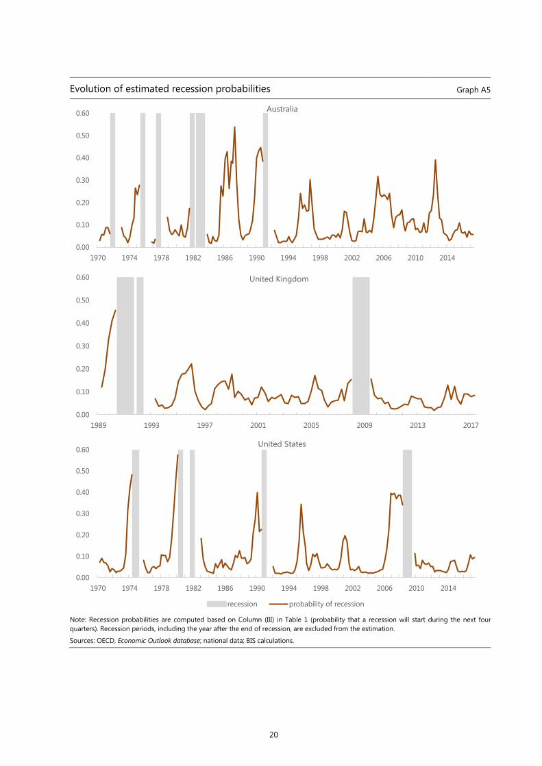
As an illustration, we plot the recession probabilities obtained from the parsimonious specification

(III) in Appendix Graph A5 for three economies: Australia, the United Kingdom and the United States. The strong rise in estimated recession probabilities prior to downturns is prominent, especially for the United States. However, similar dynamics can also be seen in the other two economies, especially for the recessions in the early 1990s, when both Australia and the United Kingdom experienced residential investment slumps.

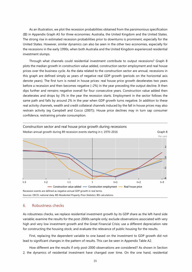
Through what channels could residential investment contribute to output recessions? Graph 8 plots the median growth in construction value added, construction sector employment and real house prices over the business cycle. As the data related to the construction sector are annual, recessions in this graph are defined simply as years of negative real GDP growth (periods on the horizontal axis denote years). The first turn is noted in house prices: real house price growth decelerates two years before a recession and then becomes negative (–2%) in the year preceding the output decline. It then dips further and remains negative overall for four consecutive years. Construction value added then decelerates and drops by 3% in the year the recession starts. Employment in the sector follows the same path and falls by around 2% in the year when GDP growth turns negative. In addition to these real activity channels, wealth and credit collateral channels induced by the fall in house prices may also restrain activity (eg Campbell and Cocco (2007)). House price declines may in turn sap consumer confidence, restraining private consumption.

Construction sector and real house price growth during recessions Median annual growth during 89 recession events starting in t, 1970–2016 Graph 8

Per cent

Recession events are defined as negative annual GDP growth in real terms.

Sources: OECD; national data; BIS Residential Property Price Statistics; BIS calculations.

6. Robustness checks

As robustness checks, we replace residential investment growth by its GDP share as the left-hand side variable; examine the results for the post-2000s sample only; exclude observations associated with very high and very low investment growth and the Great Financial Crisis; use a different depreciation rate for constructing the housing stock; and evaluate the relevance of public housing for the results.

First, replacing the dependent variable to one based on the investment to GDP growth did not lead to significant changes in the pattern of results. This can be seen in Appendix Table A2.

How different are the results if only post-2000 observations are considered? As shown in Section 2, the dynamics of residential investment have changed over time. On the one hand, residential

16

investment growth has fallen. Early in the sample, a number of countries had large government programmes to increase the supply of housing. These naturally tend to be relatively unresponsive to market conditions. On the other hand, many countries have seen financial liberalisation, reflected in increased availability of mortgages to households and reduced cost of credit.

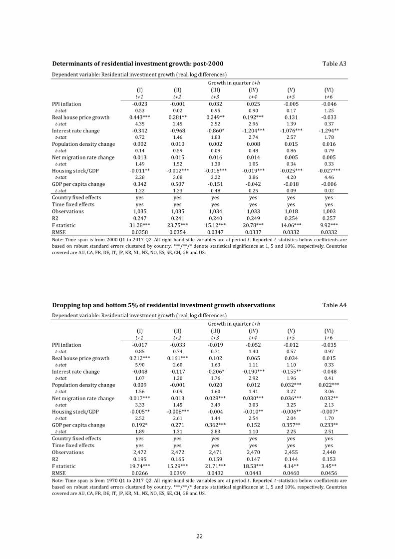
Appendix Table A3 shows that residential investment becomes more closely associated with real house prices and interest rates during the post-2000 period. The cumulative effect of a 100 basis point increase in nominal interest rates on residential investment after six quarters is –0.5% over the whole sample, but rises to –3.6% post-2000.13 Similarly, a 1% rise in house prices has a cumulative effect of 0.55% during the whole sample, but 1.2% during the more recent period. In contrast, demographic variables lose their statistical significance in the most recent period.14

Next, we examine the robustness of the results to the exclusion of more extreme investment growth observations. We remove all observations that are associated with very low or very high residential investment growth, ie the top and bottom 5% of the sample distribution. As shown in Appendix Table A4, this results in generally higher R-squared statistics. By and large, the same pattern of results reported previously persists, and changes in the size of estimated coefficients are mostly marginal. The relationship between residential investment and GDP per capita becomes stronger when outliers are excluded. On the other hand, the significance of population density falls at lower but not at higher lags.

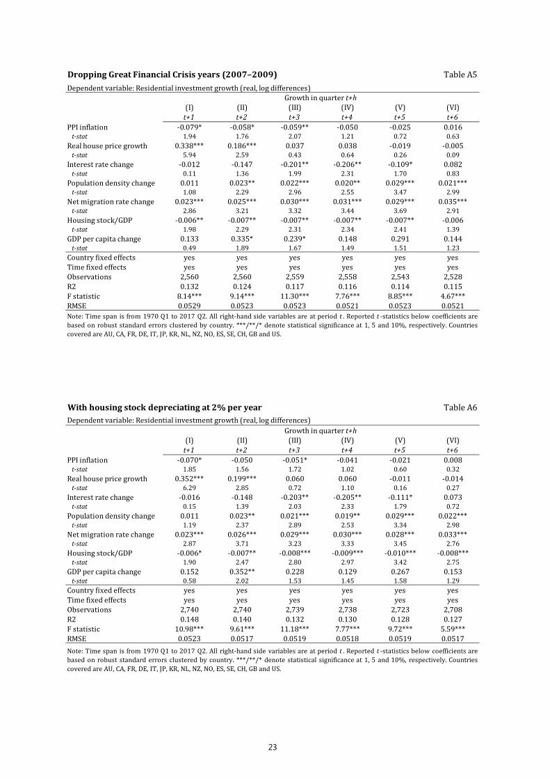
We also exclude the observations related to the Great Financial Crisis (2007–09). During these three years, all countries in the sample saw a decline in the residential investment-to-GDP ratio, ranging from 0.3 percentage points in Italy and Switzerland to 3 percentage points in Spain. Appendix Table A5 shows that the results remain largely robust to the exclusion of the GFC years, with producer price inflation rising in statistical significance, but the relevance of GDP per capita falling somewhat.

The results are little affected if we consider a depreciation rate of 2% instead of 1.5% in the construction of the housing stock (Appendix Table A6).

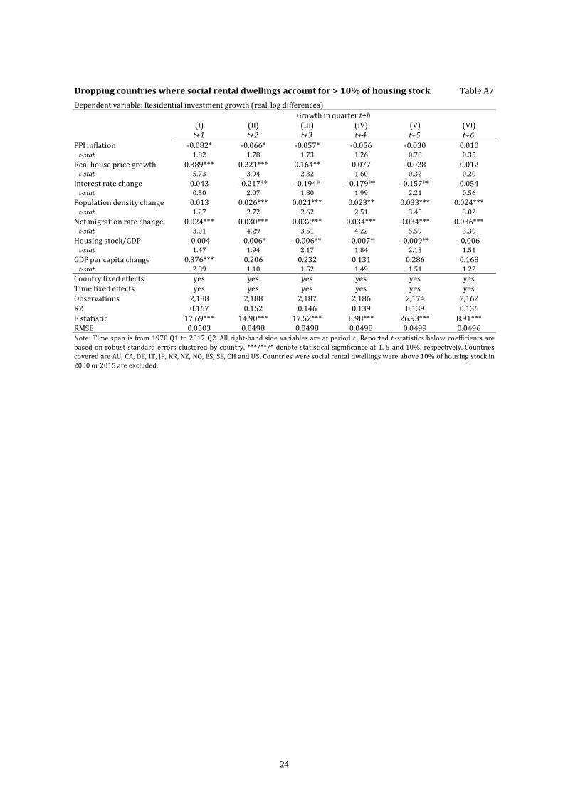
Finally, we analyse the relevance of public housing provision for the results. On the one hand, our estimated model – including determinants such as construction costs and income levels – may be more adequate for economies where public sector residential investment is less important. On the other hand, variables such as real house price growth are relevant for both private and public housing provision, through a higher Tobin’s q and the objective of guaranteeing adequate supply of low-cost housing for lower income groups. To capture the impact of public housing, we estimate the baseline model excluding all countries where social rental dwellings accounted for at least 10% of the total housing stock in both 2000 and/or 2015, ie France, the Netherlands and the United Kingdom.15

The fit of the model improves somewhat when countries with the highest public housing provision are excluded (Appendix Table A7). This is reflected in higher R-squared values, for every lag considered

13 We consider only the coefficients that are statistically significant at least at a 5% level.

14 The more recent period was also characterised by heightened policy uncertainty in many economies, in particular after the GFC. Greater uncertainty could result in the postponement of construction projects due to uncertain returns. To address this issue, we used a measure from Baker et al (2016) that is based on the frequency of newspaper articles that discuss policy uncertainty. While we found that policy uncertainty is negatively associated with residential investment activity, the magnitude was small. These results are available upon request.

15 We use data from the OECD’s Affordable Housing Database.

17

in the table. Moreover, the sensitivity of residential investment to real house prices and interest rates becomes slightly higher.

7. Conclusions

In this paper we analysed the behaviour and main drivers of residential investment using a panel dataset for 15 advanced economies since the beginning of the 1970s. Our estimations suggest that house price growth, net migration inflows and the size of the existing housing stock are the most important drivers of residential investment across various model specifications. We also found that interest rate increases affected residential investment more than interest rate decreases, and that interest rate changes had larger effects on residential investment when its share in overall GDP was rising strongly.

We also showed that residential investment consistently anticipated economic downturns, and that adding information on residential investment dynamics clearly improved the performance of standard recession prediction models.

One interesting issue for future research is the relevance of country-specific institutional factors for residential investment, such as the effect of regulations on housing supply. Such factors cannot be incorporated easily in a cross-country study but they could matter for country-specific investment dynamics. Another interesting issue relates to the use of macroprudential policies directed at the housing sector, which have gained prominence in advanced economies over the past decade. To the extent that they become widely used, macroprudential policies may affect the short-term dynamics of residential investment activity in the future.

18

Appendix

Construction employment generally highest before the 1990s, fell post-crisis As per cent of total employment Graph A1

1 Period averages of annual data. For New Zealand, data are available from 1978.


GDP falls by more than its residential investment component during recessions Median growth during 99 recession events starting in t, 1970–2016 Graph A2

Per cent

Recession events are defined as at least two consecutive quarters of negative GDP growth based on seasonally adjusted data.


19

Residential investment versus GDP growth during recessions Average changes (coefficient 𝛽𝛽) during 99 recession events starting in t, 1970-2016 Graph A3

Percentage points

This graph estimates the average changes of residential investment and GDP growth during eight quarters before and after 99 recession events relative to normal times, controlling for country and time fixed effects. The regression is of the type:

𝐼𝐼𝐼𝐼𝐼𝐼 𝑜𝑜𝑜𝑜 𝐺𝐺𝐺𝐺𝐺𝐺 𝑔𝑔𝑜𝑜𝑜𝑜𝑔𝑔𝑔𝑔ℎ𝑖𝑖=𝑐𝑐𝑜𝑜𝑐𝑐𝑐𝑐𝑔𝑔𝑜𝑜𝑐𝑐,𝑡𝑡=𝑡𝑡𝑖𝑖𝑡𝑡𝑡𝑡,𝑟𝑟𝑡𝑡𝑟𝑟=𝑠𝑠𝑡𝑡𝑠𝑠𝑟𝑟𝑡𝑡 𝑜𝑜𝑜𝑜 𝑟𝑟𝑡𝑡𝑟𝑟𝑡𝑡𝑠𝑠𝑠𝑠𝑖𝑖𝑜𝑜𝑟𝑟 = � 𝛽𝛽𝑘𝑘8

𝑘𝑘=−81𝑡𝑡=𝑟𝑟𝑡𝑡𝑟𝑟+𝑘𝑘 + 𝛾𝛾𝑖𝑖 + 𝛿𝛿𝑡𝑡 + 𝜀𝜀𝑖𝑖,𝑡𝑡,𝑟𝑟𝑡𝑡𝑟𝑟

The ranges indicate the 95% confidence intervals.


Global factor in residential investment growth Time fixed effect from residential investment regression Graph A4

The time fixed effect is based on the regression in Column (1) of Table 2 and is shown in the graph as the four-quarter moving average.


-0.03

-0.02

-0.01

0

0.01

0.02

0.03

1972 1976 1980 1984 1988 1992 1996 2000 2004 2008 2012 2016

20

Evolution of estimated recession probabilities Graph A5

Note: Recession probabilities are computed based on Column (III) in Table 1 (probability that a recession will start during the next four quarters). Recession periods, including the year after the end of recession, are excluded from the estimation.


0.00

0.10

0.20

0.30

0.40

0.50

0.60

1970 1974 1978 1982 1986 1990 1994 1998 2002 2006 2010 2014

Australia

0.00

0.10

0.20

0.30

0.40

0.50

0.60

1989 1993 1997 2001 2005 2009 2013 2017

United Kingdom

0.00

0.10

0.20

0.30

0.40

0.50

0.60

1970 1974 1978 1982 1986 1990 1994 1998 2002 2006 2010 2014

United States

recession probability of recession

21

Specification without time fixed effects Table A1

Dependent variable: Residential investment growth (real, log differences)


PPI inflation -0.094*** -0.082*** -0.082*** -0.071*** -0.057*** -0.035* t-stat 3.94 4.29 4.84 3.93 3.19 1.83Real house price growth 0.397*** 0.228*** 0.081 0.069 -0.016 -0.056 t-stat 6.41 3.92 1.19 1.13 0.25 0.94Interest rate change -0.113 -0.274** -0.270** -0.215** -0.104* -0.020 t-stat 0.88 2.25 2.08 1.97 1.74 0.24Population density change 0.009 0.020* 0.017** 0.016* 0.020* 0.016 t-stat 1.04 1.94 1.98 1.75 1.91 1.57Net migration rate change 0.020*** 0.024*** 0.028*** 0.029*** 0.029*** 0.032*** t-stat 2.86 3.44 3.54 3.68 3.59 2.88Housing stock/GDP -0.008*** -0.008*** -0.009*** -0.009*** -0.008*** -0.006*** t-stat 2.54 2.62 4.38 4.32 4.09 3.19GDP per capita change 0.263 0.260* 0.057 -0.036 0.012 -0.017 t-stat 1.12 1.65 0.46 0.36 0.08 0.13Country fixed effects yes yes yes yes yes yesTime fixed effects no no no no no noObservations 2,740 2,740 2,739 2,738 2,723 2,708R2 0.060 0.042 0.028 0.023 0.017 0.016F statistic 11.67*** 14.21*** 9.27*** 11.73*** 18.27*** 9.55***RMSE 0.0530 0.0527 0.0530 0.0530 0.0532 0.0530


Note: Time span is from 1970 Q1 to 2017 Q2. All right-hand side variables are at period t . Reported t -statistics below coefficients arebased on robust standard errors clustered by country. ***/**/* denote statistical significance at 1, 5 and 10%, respectively. Countriescovered are AU, CA, FR, DE, IT, JP, KR, NL, NZ, NO, ES, SE, CH, GB and US.

Determinants of residential investment to GDP ratio Table A2

Dependent variable: Residential investment to GDP (differences)


PPI inflation -0.062* -0.045 -0.052* -0.040 -0.018 0.006 t-stat 1.67 1.45 1.81 0.97 0.52 0.27Real house price growth 0.295*** 0.159** 0.055 0.051 -0.004 -0.001 t-stat 6.02 2.37 0.68 0.97 0.06 0.01Interest rate change -0.014 -0.100 -0.166* -0.196** -0.069 0.072 t-stat 0.14 1.05 1.89 2.54 1.13 0.78Population density change 0.031 0.013 0.013** 0.013** 0.022*** 0.016** t-stat 0.32 1.48 2.20 2.00 2.91 2.21Net migration rate change 0.016** 0.021*** 0.024*** 0.022*** 0.020*** 0.023** t-stat 2.24 2.62 2.69 2.72 2.81 2.32Housing stock/GDP -0.005* -0.006*** -0.007*** -0.008*** -0.009*** -0.007** t-stat 1.77 3.06 3.52 2.67 3.06 2.47GDP per capita change 0.156 0.273 0.067 0.147* 0.213 0.072 t-stat 0.59 1.44 0.51 1.91 1.26 0.49Country fixed effects yes yes yes yes yes yesTime fixed effects yes yes yes yes yes yesObservations 2,740 2,740 2,725 2,710 2,695 2,680R2 0.121 0.113 0.108 0.108 0.105 0.104F statistic 12.75*** 5.97*** 10.00*** 5.64*** 5.50*** 4.47***RMSE 0.0508 0.0502 0.0504 0.0504 0.0505 0.0503



22

Determinants of residential investment growth: post-2000 Table A3Dependent variable: Residential investment growth (real, log differences)


PPI inflation -0.023 -0.001 0.032 0.025 -0.005 -0.046 t-stat 0.53 0.02 0.95 0.90 0.17 1.25Real house price growth 0.443*** 0.281** 0.249** 0.192*** 0.131 -0.033 t-stat 4.35 2.45 2.52 2.96 1.39 0.37Interest rate change -0.342 -0.968 -0.860* -1.204*** -1.076*** -1.294** t-stat 0.72 1.46 1.83 2.74 2.57 1.78Population density change 0.002 0.010 0.002 0.008 0.015 0.016 t-stat 0.14 0.59 0.09 0.48 0.86 0.79Net migration rate change 0.013 0.015 0.016 0.014 0.005 0.005 t-stat 1.49 1.52 1.30 1.05 0.34 0.33Housing stock/GDP -0.011** -0.012*** -0.016*** -0.019*** -0.025*** -0.027*** t-stat 2.28 3.08 3.22 3.86 4.20 4.46GDP per capita change 0.342 0.507 -0.151 -0.042 -0.018 -0.006 t-stat 1.22 1.23 0.48 0.25 0.09 0.02Country fixed effects yes yes yes yes yes yesTime fixed effects yes yes yes yes yes yesObservations 1,035 1,035 1,034 1,033 1,018 1,003R2 0.247 0.241 0.240 0.249 0.254 0.257F statistic 31.28*** 23.75*** 15.12*** 20.78*** 14.06*** 9.92***RMSE 0.0358 0.0354 0.0347 0.0337 0.0332 0.0332



Dropping top and bottom 5% of residential investment growth observations Table A4Dependent variable: Residential investment growth (real, log differences)


PPI inflation -0.017 -0.033 -0.019 -0.052 -0.012 -0.035 t-stat 0.85 0.74 0.71 1.40 0.57 0.97Real house price growth 0.212*** 0.161*** 0.102 0.065 0.034 0.015 t-stat 5.90 2.60 1.63 1.11 1.10 0.33Interest rate change -0.048 -0.117 -0.206* -0.190*** -0.155** -0.048 t-stat 1.07 1.20 1.76 2.92 1.96 0.41Population density change 0.009 -0.001 0.020 0.012 0.032*** 0.022*** t-stat 1.56 0.09 1.60 1.41 3.27 3.06Net migration rate change 0.017*** 0.013 0.028*** 0.030*** 0.036*** 0.032** t-stat 3.33 1.45 3.49 3.03 3.25 2.13Housing stock/GDP -0.005** -0.008*** -0.004 -0.010** -0.006** -0.007* t-stat 2.52 2.61 1.44 2.54 2.04 1.70GDP per capita change 0.192* 0.271 0.362*** 0.152 0.357** 0.233** t-stat 1.89 1.31 2.83 1.10 2.25 2.51Country fixed effects yes yes yes yes yes yesTime fixed effects yes yes yes yes yes yesObservations 2,472 2,472 2,471 2,470 2,455 2,440R2 0.195 0.165 0.159 0.147 0.144 0.153F statistic 19.74*** 15.29*** 21.71*** 18.53*** 4.14** 3.45**RMSE 0.0266 0.0399 0.0432 0.0443 0.0460 0.0456



23

Dropping Great Financial Crisis years (2007–2009) Table A5Dependent variable: Residential investment growth (real, log differences)


PPI inflation -0.079* -0.058* -0.059** -0.050 -0.025 0.016 t-stat 1.94 1.76 2.07 1.21 0.72 0.63Real house price growth 0.338*** 0.186*** 0.037 0.038 -0.019 -0.005 t-stat 5.94 2.59 0.43 0.64 0.26 0.09Interest rate change -0.012 -0.147 -0.201** -0.206** -0.109* 0.082 t-stat 0.11 1.36 1.99 2.31 1.70 0.83Population density change 0.011 0.023** 0.022*** 0.020** 0.029*** 0.021*** t-stat 1.08 2.29 2.96 2.55 3.47 2.99Net migration rate change 0.023*** 0.025*** 0.030*** 0.031*** 0.029*** 0.035*** t-stat 2.86 3.21 3.32 3.44 3.69 2.91Housing stock/GDP -0.006** -0.007** -0.007** -0.007** -0.007** -0.006 t-stat 1.98 2.29 2.31 2.34 2.41 1.39GDP per capita change 0.133 0.335* 0.239* 0.148 0.291 0.144 t-stat 0.49 1.89 1.67 1.49 1.51 1.23Country fixed effects yes yes yes yes yes yesTime fixed effects yes yes yes yes yes yesObservations 2,560 2,560 2,559 2,558 2,543 2,528R2 0.132 0.124 0.117 0.116 0.114 0.115F statistic 8.14*** 9.14*** 11.30*** 7.76*** 8.85*** 4.67***RMSE 0.0529 0.0523 0.0523 0.0521 0.0523 0.0521



With housing stock depreciating at 2% per year Table A6Dependent variable: Residential investment growth (real, log differences)


PPI inflation -0.070* -0.050 -0.051* -0.041 -0.021 0.008 t-stat 1.85 1.56 1.72 1.02 0.60 0.32Real house price growth 0.352*** 0.199*** 0.060 0.060 -0.011 -0.014 t-stat 6.29 2.85 0.72 1.10 0.16 0.27Interest rate change -0.016 -0.148 -0.203** -0.205** -0.111* 0.073 t-stat 0.15 1.39 2.03 2.33 1.79 0.72Population density change 0.011 0.023** 0.021*** 0.019** 0.029*** 0.022*** t-stat 1.19 2.37 2.89 2.53 3.34 2.98Net migration rate change 0.023*** 0.026*** 0.029*** 0.030*** 0.028*** 0.033*** t-stat 2.87 3.71 3.23 3.33 3.45 2.76Housing stock/GDP -0.006* -0.007** -0.008*** -0.009*** -0.010*** -0.008*** t-stat 1.90 2.47 2.80 2.97 3.42 2.75GDP per capita change 0.152 0.352** 0.228 0.129 0.267 0.153 t-stat 0.58 2.02 1.53 1.45 1.58 1.29Country fixed effects yes yes yes yes yes yesTime fixed effects yes yes yes yes yes yesObservations 2,740 2,740 2,739 2,738 2,723 2,708R2 0.148 0.140 0.132 0.130 0.128 0.127F statistic 10.98*** 9.61*** 11.18*** 7.77*** 9.72*** 5.59***RMSE 0.0523 0.0517 0.0519 0.0518 0.0519 0.0517



24

Dropping countries where social rental dwellings account for > 10% of housing stock Table A7Dependent variable: Residential investment growth (real, log differences)


PPI inflation -0.082* -0.066* -0.057* -0.056 -0.030 0.010 t-stat 1.82 1.78 1.73 1.26 0.78 0.35Real house price growth 0.389*** 0.221*** 0.164** 0.077 -0.028 0.012 t-stat 5.73 3.94 2.32 1.60 0.32 0.20Interest rate change 0.043 -0.217** -0.194* -0.179** -0.157** 0.054 t-stat 0.50 2.07 1.80 1.99 2.21 0.56Population density change 0.013 0.026*** 0.021*** 0.023** 0.033*** 0.024*** t-stat 1.27 2.72 2.62 2.51 3.40 3.02Net migration rate change 0.024*** 0.030*** 0.032*** 0.034*** 0.034*** 0.036*** t-stat 3.01 4.29 3.51 4.22 5.59 3.30Housing stock/GDP -0.004 -0.006* -0.006** -0.007* -0.009** -0.006 t-stat 1.47 1.94 2.17 1.84 2.13 1.51GDP per capita change 0.376*** 0.206 0.232 0.131 0.286 0.168 t-stat 2.89 1.10 1.52 1.49 1.51 1.22Country fixed effects yes yes yes yes yes yesTime fixed effects yes yes yes yes yes yesObservations 2,188 2,188 2,187 2,186 2,174 2,162R2 0.167 0.152 0.146 0.139 0.139 0.136F statistic 17.69*** 14.90*** 17.52*** 8.98*** 26.93*** 8.91***RMSE 0.0503 0.0498 0.0498 0.0498 0.0499 0.0496


Note: Time span is from 1970 Q1 to 2017 Q2. All right-hand side variables are at period t . Reported t -statistics below coefficients arebased on robust standard errors clustered by country. ***/**/* denote statistical significance at 1, 5 and 10%, respectively. Countriescovered are AU, CA, DE, IT, JP, KR, NZ, NO, ES, SE, CH and US. Countries were social rental dwellings were above 10% of housing stock in2000 or 2015 are excluded.

25

References

Agnello, L and L Schuknecht (2011): “Booms and busts in housing markets: determinants and implications”, Journal of Housing Economics, vol. 20, 3, pp 171–90.

Angrist, J, O Jorda and G Kuersteiner (2013): “Semiparametric estimates of monetary policy effects: string theory revisited“, NBER Working Paper, no 19355.

Aspachs-Bracons, O and P Rabanal (2011): “The effects of housing prices and monetary policy in a currency union“, International Journal of Central Banking, vol. 7, 1, pp 225–74.

Baker, S, N Bloom and S Davis (2016): “Measuring economic policy uncertainty”, The Quarterly Journal of Economics, vol. 131, 4, pp 1593–636.

Borio, C (2014): “The financial cycle and macroeconomics: what have we learnt?” Journal of Banking and Finance, vol 45, pp 182–98.

Calza, A, T Monacelli and L Stracca (2013): “Housing finance and monetary policy”, Journal of the European Economic Association, vol 11, pp 101–22.

Campbell, J and J Cocco (2007): "How do house prices affect consumption? Evidence from micro data", Journal of Monetary Economics, vol 54, pp 591–621.

Claessens, S and M Kose (2018): “Frontiers of macrofinancial linkages”, BIS Papers, no 95.

Claessens, S, M Kose and M Terrones (2012): “How do business and financial cycles interact?” Journal of International Economics, vol 87, pp 178–190.

Corder, M (2008): “Understanding dwellings investment”, Bank of England Quarterly Bulletin, Q4.

Davis, M and J Heathcote (2005): “Housing and the business cycle“, International Economic Review, vol 46.

Dokko, J, B Doyle, M Kiley, J Kim, S Sherlund, J Sim and S van den Heuvel (2011): “Monetary policy and the global housing bubble”, Economic Policy, vol 26, pp 237–87.

Emanuelsson, R (2015): “Supply of housing in Sweden”, Sveriges Riksbank Economic Review, no 2, pp 47–75.

Erceg, C and A Levin (2006): “Optimal monetary policy with durable consumption goods”, Journal of Monetary Economics, vol 53, pp 1341–59.

Estrella, A and G A Hardouvelis (1991): “The term structure as a predictor of real economic activity”, Journal of Finance, vol. 46, pp 555–76.

Garcia-Herrero, A and S Fernandez de Lis (2008): “The housing boom and bust in Spain: impact of the securitisation model and dynamic provisioning”, BBVA Working Papers, no 806.

Glaeser, E and J Gyourko (2007): “Housing dynamics”, Harvard Institute of Economic Research Discussion Papers, no 2137.

Glaeser, E, J Gyourko and A Saiz (2008): “Housing supply and housing bubbles”, Journal of Urban Economics, vol 64, pp 198–217.

Iacoviello, M (2005): “House prices, borrowing constraints, and monetary policy in the business cycle”, American Economic Review, vol 95, pp 739–764.

Iacoviello, M and S Neri (2010): “Housing market spillovers: evidence from an estimated DSGE model”, American Economic Journal: Macroeconomics, vol 2, pp 125–164.

International Monetary Fund (2008): “The changing housing cycle and the implications for monetary policy”, World Economic Outlook, Chapter 3, April.

Jarocinski, M and F Smets (2008): “House prices and the stance of monetary policy”, Federal Reserve Bank of St. Louis Review, July, pp 339–66.

26

Jordà, O (2005): “Estimation and inference of impulse responses by local projections”, American Economic Review, vol 95, pp 161–82.

Jordà, O, M Schularick and A Taylor (2016): “The great mortgaging: housing finance, crises and business cycles”, Economic Policy, pp 107–251.

Kydland, F and E Prescott (1982): “Time to build and aggregate fluctuations”, Econometrica, vol 50, pp 1345–70.

Leamer, E (2007): “Housing is the business cycle”, Proceedings - Economic Policy Symposium - Jackson Hole, Federal Reserve Bank of Kansas City, pp 149–233.

Leamer, E (2015): “Housing really is the business cycle: what survives the lessons of 2008–09?”, Journal of Money, Credit and Banking, vol 47, pp 43–50.

McCarthy, J and R W Peach (2002): “Monetary policy transmission to residential investment“, Federal Reserve Bank of New York Economic Policy Review, vol 8, pp 139–58.

Mishkin, F (2007): “Housing and the monetary transmission mechanism”, NBER Working Papers, no 13518.

Piketty, T and G Zucman (2014): “Capital is back: wealth-income ratios in rich countries 1700–2010”, Quarterly Journal of Economics, vol 129, 3, pp 1255–310.

Poterba, J (1984): “Tax subsidies to owner-occupied housing: an asset-market approach“, Quarterly Journal of Economics, vol 99, pp 729–52.

Rognlie, M, A Shleifer and A Simsek (2018): “Investment hangover and the great recession“, American Economic Journal: Macroeconomics (forthcoming).

Rudebusch, G and J Williams (2009): “Forecasting recessions: the puzzle of the enduring power of the yield curve”, Journal of Business and Economic Statistics, vol 27, pp 492–503.

Scatigna, M, R Szemere and K Tsatsaronis (2014): “Residential property price statistics across the globe”, BIS Quarterly Review, September, pp 61–76.

Sutton, G, D Mihaljek and A Subelyte (2017): “Interest rates and house prices in the United States and around the world”, BIS Working Papers, no 665, October.

Taylor J B (2007): “Housing and monetary policy“, NBER Working Paper, no 13682.

Tenreyro, S and G Thwaites (2016): “Pushing on a string: US monetary policy is less powerful in recessions“, American Economic Journal: Macroeconomics, vol 8, pp 43–74.

Topel, R and S Rosen (1988): “Housing investment in the United States”, Journal of Political Economy, vol 96, pp 718-740.

Tsoukis, C and P Westaway (1994): “A forward looking model of housing construction in the UK”, Economic Modelling, vol 11, 2, pp 266–79.

Vavra, J (2014): “Inflation dynamics and time-varying volatility: new evidence and an Ss interpretation”, Quarterly Journal of Economics, vol 129, pp 215–58.

https://www.dropbox.com/s/cn8ici8pa8ypbfo/AEJMacro-2016-0211_manuscript.pdf?dl=0

https://www.dropbox.com/s/cn8ici8pa8ypbfo/AEJMacro-2016-0211_manuscript.pdf?dl=0

Previous volumes in this series

725 May 2018

Identifying oil price shocks and their consequences: the role of expectations in the crude oil market

Takuji Fueki , Hiroka Higashi , Naoto Higashio , Jouchi Nakajima , Shinsuke Ohyama and Yoichiro Tamanyu

724 May 2018

Do small bank deposits run more than large ones? Three event studies of contagion and financial inclusion

Dante B Canlas, Johnny Noe E Ravalo and Eli M Remolona

723 May 2018

The cross-border credit channel and lending standards surveys

Andrew Filardo and Pierre Siklos

722 May 2018

The enduring link between demography and inflation

Mikael Juselius and Előd Takáts

721 May 2018

Effects of asset purchases and financial stability measures on term premia in the euro area

Richhild Moessner

720 May 2018

Could a higher inflation target enhance macroeconomic stability?

José Dorich, Nicholas Labelle St-Pierre, Vadym Lepetyuk and Rhys R. Mendes

719 May 2018

Channels of US monetary policy spillovers to international bond markets

Elias Albagli, Luis Ceballos, Sebastian Claro, and Damian Romero

718 May 2018

Breaking the trilemma: the effects of financial regulations on foreign assets

David Perez-Reyna and Mauricio Villamizar-Villegas

717 May 2018

Financial and price stability in emerging markets: the role of the interest rate

Lorenzo Menna and Martin Tobal

716 April 2018

Macro-financial linkages: the role of liquidity dependence

Alexey Ponomarenko, Anna Rozhkova and Sergei Seleznev

715 April 2018

A time series model of interest rates with the effective lower bound

Benjamin K Johannsen and Elmar Mertens

714 April 2018

Do interest rates play a major role in monetary policy transmission in China?

Güneş Kamber and Madhusudan Mohanty

713 April 2018

Inflation and professional forecast dynamics: an evaluation of stickiness, persistence, and volatility

Elmar Mertens and James M. Nason

711 March 2018

Credit supply and productivity growth Francesco Manaresi and Nicola Pierri

All volumes are available on our website www.bis.org.

http://www.bis.org/

Documents

BIS Working Papers · Keywords: housing markets, residential investment , house prices, business cycle s, construction, interest rates, recession forecasts : ... demographic factors