Biophysical Analyses Final Report For Study the changes to ... · Biophysical Analyses Final ... APPENDIX-Q Summary Statistics based on Sample Data of Bani Hashem ... Ms. Samia Bakheit

1

Biophysical Analyses Final Report

For

Study the changes to Ecosystem Services

Following the

Implementation of Sustainable Land Use Practices

Submitted to

Global Economics Programme of International Union of Conservation for Nature (IUCN)

And

Global Ecosystem Management Program – Global Drylands Initiatives (IUCN)

By

Dr. Moe Myint Chief Scientist, MNRII

Biophysical Consultant to IUCN

17 July 2014

Gland, Switzerland

2

Table of Contents

Acknowledgement .......................................................................................................................... 5

Executive Summary ..................................................................................................................... 6

1. Introduction ................................................................................................................................ 8

2. Methodology ............................................................................................................................... 9

3. Current Land Use and Land Cover Mapping ............................................................................. 12

3.1 Present Land Use and Land Cover Mapping at study watershed in Jordan ....................... 13

3.2 Present Land Use and Land Cover Mapping at study watershed in Sudan ........................ 14

3.3 Present Land Use and Land Cover Mapping at study watershed in Mali ........................... 15

4. Future Land Use and Land Cover Mapping ............................................................................... 16

4.1 Criteria for Future Land Use and Land Cover Mapping at study watershed in Jordan ....... 16

4.2 Criteria for Future Land Use and Land Cover Mapping at study watershed in Sudan ....... 18

4.3 Criteria for Future Land Use and Land Cover Mapping at study watershed in Mali .......... 19

5. Scenario Modeling using ArcSWAT .......................................................................................... 20

5.1 Analyses of Scenario Modeling Result for study watershed in Mali ................................... 21

5.2 Analyses of Scenario Modeling Result for Study watershed in Sudan ............................... 24

5.3 Analyses of Scenario Modeling Result for Study watershed in Jordan ............................... 26

6. Biomass Estimation in rangeland for study watershed in Jordan ............................................ 34

6.1 Estimation of Biomass Per Ha in Open Access Rangeland and Hima System ..................... 34

6.2 Future HIMA system restoration scenario .......................................................................... 34

6.3 Baseline Scenario for Hima Development .......................................................................... 38

7. Biomass Estimation and Carbon Sequestration for study watershed in Mali .......................... 40

7.1 Literature review in relation to Acacia Nilotica .................................................................. 40

7.2 Literature review in relation to Acacia Raddiana ................................................................ 41

7.3 Literature review in relation to Acacia Albida ..................................................................... 41

7.4 Biomass estimation of Acacia Nilotica at the specific age .................................................. 42

7.5 Biomass Estimation of Acacia Raddiana at specific age ...................................................... 43

7.6 Biomass Estimation of Acacia Albida at specific age ........................................................... 44

7.7 Biomass estimation of Acacia Nilotica until 30 years old ................................................... 45

7.8 Biomass estimation of Acacia Raddiana until 30 years old ................................................. 46

3

7.9 Biomass estimation of Acacia Albida until 30 years old...................................................... 47

References .................................................................................................................................... 49

Web Reference ............................................................................................................................. 50

Appendix-A Study Area and its watershed in Zarqa River Basin, Jordan...................................... 51

Appendix-B Study Area and its watershed in Al Gadaref State, Sudan ........................................ 52

Appendix-C Study Area and its watershed near Mopti Region, Mali ........................................... 53

Appendix-D Present Land Use and Land Cover Map of Study watershed in Jordan .................... 54

Appendix-E Present Land Use and Land Cover Map of Study watershed in Sudan ..................... 55

Appendix-F Present Land Use and Land Cover Map of Study watershed in Mali ........................ 56

Appendix-G Suitable Areas for Hima Development in the study watershed of Jordan ............... 57

Appendix-H Future Scenario Land use and land cover Map of study watershed in Jordan ........ 58

Appendix-I Spatial Distribution of Hima and Open Access Rangelands ....................................... 59

Appendix-J Future Scenario Land Use and Land Cover Map of study watershed in Sudan ......... 60

Appendix-K Future Scenario Land use and land cover Map of study watershed in Mali ............. 61

Appendix-L: Mathematical Formulation of Water Balance .......................................................... 62

Appendix-M SWAT Model Parameters for Africa referred by the project ................................... 65

APPENDIX-N National Estimates of available water in Africa ....................................................... 66

APPENDIX-O Comparison of results from Published Africa Study to ArcSWAT output for Mali .. 67

APPENDIX-P Comparison of results from Published Africa Study to ArcSWAT output for Suda . 68

APPENDIX-Q Summary Statistics based on Sample Data of Bani Hashem Hima Sites ................. 69

APPENDIX-R Estimating Fresh Biomass to Dry Biomass and Biomass (Kg) Per Ha for Hima and

Open Access rangeland ................................................................................................................. 70

APPENDIX-S Biodiverse Biomass Accumulation from cdm.unfccc.int .......................................... 71

APPENDIX –T: Ratios of biomass increment based on Biodiverse Biomass Accumulation .......... 72

APPENDIX-U Annual Biomass Accumulation and Carbon Sequestration by Acacia Nilotica ....... 73

APPENDIX-V Annual Biomass Accumulation and Carbon Sequestration by Acacia Raddiana ..... 74

APPENDIX-W Annual Biomass Accumulation and Carbon Sequestration by Acacia Albida ......... 75

APPENDIX – X Digital Elevation Model of the study area watershed of Jordan ........................... 76

APPENDIX – Y Digital Elevation Model of the study area watershed of Sudan ............................ 77

APPENDIX-Z Digital Elevation Model of the study area watershed of Mali ................................. 78

4

APPENDIX – AA FAO Soil Map of the study area watershed of Jordan ........................................ 79

APPENDIX – AB FAO Soil Map of the study area watershed of Sudan ......................................... 80

APPENDIX – AC FAO Soil Map of the study area watershed of Mali ............................................ 81

APPENDIX-AD Daily Weather data description for the study areas of Jordan, Sudan and Mali .. 82

APPENDIX – AE Monthly Weather Data of Mopti Weather Station for the Study Area of Mali .. 83

5

Acknowledgement

First and foremost, the author would like to express his profound gratitude and indebtedness to

Nathalie Olsen and Vanja Westerberg of Global Economics Programme of International Union of

Conservation for Nature (IUCN) for initiating, facilitation and providing an opportunity for conducting

the biophysical research on quantification of impacts on ecosystem and changes in ecosystem services

due to policy changes for economic valuation.

The author is very grateful to Edmund Barrow, Jonathan Davies, Masumi Gudka and Akshay Vishwanath

of Global Ecosystem Management Program, Eastern and Southern Africa Regional Office (ESARO) IUCN

for suggestions, guidance, advice for planning the field work in Sudan and financial support for

conducting this research study.

The author gratefully acknowledges Fidaa F. Haddad, Moath Hasan and Diab Sulimamn of Regional

Office for West Africa (ROWA) IUCN for hospitality, organizing and facilitating meetings with

government agencies, and accompanying during the field work at Zarqa River Basin in Jorden.

I would like to thank Dr. Osman Omer Abdalla, Chief Technical Director of Forest National Corporation (FNC) for facilitation and kind support during my field visit to Al Gadaref State, Sudan. The contribution and facilitation from Mr. Isam Abdelkarim Mohamed, Project Manager of FNC, Ms. Nada Ibrahim Mohamed Extension Officer, Mr. Abdel Bagi, Mr. Mohammad Ahmed Arbab, Mr. Yousif Hassan, Ms. Rasha Bashir, Ms. Samia Bakheit Mando and GIS staffs from Forest National Corporation are very valuable for the success of the field work in Sudan. The author really appreciates Susan Mills of Global Ecosystem Management Program IUCN for the efficient logistics supports, advice on support documents for contract signing and financial planning for field works. Finally the author would like to extend special thanks to Laurent Schmid of Global Finance Program IUCN for providing the advance for Sudan field trip within the very short notice period.

6

Executive Summary

Three watersheds from Jordan, Sudan and Mali were selected in order to study the changes to

ecosystem services following the implementation of sustainable land use practices.

Present Land Use and Land Cover Data were created using Landsat-8 2013 satellite images. Future Land

Use and Land Cover Scenario Data were created based on the existing land use policy, multidisciplinary

discussion, local expert knowledge of rangeland and forestry, biophysical suitability of proposed

restoration scenario in relation to Hima Development in Jordan, integration of shelterwood system with

Acacia Senegal and Acacia Seyal at the 10% of agriculture lands in Sudan and integration of agroforestry

and reforestation with forest plantations with Acacia Albida, Acacia Raddiana and Acacia Nilotica in Mali.

Soil and Water Assessment Tool – SWAT is a river basin, or watershed scale physical modal developed to

predict impact of land management practices on water, sediment, and agricultural chemical yields in

large, complex watersheds with varying soils, land use, and management conditions over long time.

SWAT was applied for scenario modeling for present and future land use to evaluate the impact on

water yield, surface runoff, sediment loading, aquifer recharge and important hydrological components.

In the watershed of Mali, with the future land use scenario, the total water yield will increase at the rate

of ADDITIONAL 89.8 m3 per ha. The surface run off will decrease at the rate of 110.9 m3 per hectare.

More ground water recharge at the rate of ADDITIONAL 197.7 m3 per ha which could be available by the

water depression areas in summer. Plants will get more water from shallow aquifer at the rate of

ADDITIONAL 21.2 m3 per hectare from the shallow aquifer. Total aquifer recharge will decrease at the

rate of 59.5 m3 per Ha because of more trees on the landscape. Deep Aquifer Recharge will decrease at

the rate of 278.5 m3/ha which prevent the permanent water loss. However more Ground water

recharge at the rate of ADDITIONAL 197.7 m3 per ha which could be available by the water depression

areas in summer and to the plants from the shallow aquifer to plants.

In the watershed of Sudan, with the future land use scenario with increase tree cover, there will be less

sediment loading at the rate of ADDITIONAL 0.47 tons/ha. More ground water recharge at the rate of

ADDITIONAL 36.90 m3 per ha which could be available by the water depression areas in summer. Plants

will get more water from shallow aquifer at the rate of ADDITIONAL 15.3 m3 per hectare from the

shallow aquifer. Water percolation will increase at the rate of ADDITIONAL 46.9 m3 per hectare. Total

aquifer recharge will increase at the rate of ADDITIONAL 56.4 m3 per Ha.

In the watershed of Jordan, with the future land use scenario, there will be less sediment loading at the

rate of 0.58 tons/ha. More ground water recharge at the rate of ADDITIONAL 24.20 m3 per ha which

could be partly available by the water depression areas in summer. Plants will get more water at the

rate of ADDITIONAL 2.7 m3 per hectare from the shallow aquifer. Surface runoff will decrease at the

rate of 53.3 m3/ha due to more percolation, shallow aquifer recharge, more lateral flow and deep

aquifer recharge.

The future land use scenarios in three study sites performed ecologically and hydrologically from the

sustainable land management and ecosystem function aspects while providing the better ecosystem

services to the community.

7

Noy-Meir growth function was applied to estimate the Biomass accumulation in Hima System and Open

Access Rangeland of the study area in Jordan. The spatial distribution of Hima and Open Access Plots are

allocated within 1 KM proximity to each other for easy migration of the livestock from one area to

another. This study estimated - combined mean Biomass (Tons)/Ha of Hima and Open Plots in Hima

system could reach 0.24 Tons/Ha. The minimum combined mean Biomass (Tons/Ha) of Hima Plots and

Open Access Plots is 0.09 Tons/Ha in 2013 and that of maximum is 0.24 Tons/Ha in 2038 depending on

the actual range vegetation content within each Hima and Open Access plots.

Biomass and Carbon Sequestration of Acacia Nilotica and Acacia Raddiana at 3m by 3 m spacing, Acacia

Albida at 6m by 6m spacing in the watershed of Mali is estimated annual basis based on published

research data and Biodiverse Biomass Accumulation of UNFCCC for estimating the Mean Annual

Increment (MAI) of biomass. The result will be more accurate if species specific and location specific MAI

data is available in the future.

The total biomass accumulation is 28.14 million tons and total carbon sequestration is 14.07 million tons for the 80803.9 ha of Acacia Nilotica 3m X 3m plantations in the study area of Mali at the biomass accumulation rate of 348.23 tons/ha at the 30 years age of plantation. The total biomass accumulation is 15.59 million tons and total carbon sequestration is 7.79 million tons for the 62765.36 ha of Acacia Raddiana at 3m X 3m plantations in the study area of Mali at the biomass accumulation rate of 248.38 tons/ha at the 30 years age of plantation. The total biomass accumulation is 2.83 million tons and total carbon sequestration is 1.42 million tons for the 29314.99 ha of Acacia Albida at 6m X 6m agroforestry development in the study area of Mali at the biomass accumulation rate of 96.57 tons/ha at the 30 years age of plantation. This study focused the quantification of impacts on ecosystem and changes in ecosystem services by the policy change on land use planning. Moreover, it highlights the tools and data for quantification of impacts on ecosystem and changes in ecosystem services at the landscape scale. This study bridged the biophysical science to the economic valuation of ecosystem services for the benefits of people and sustainable land management at the landscape scale.

8

1. Introduction

Three watersheds from Jordan, Sudan and Mali were selected in order to study the changes to

ecosystem services following the implementation of sustainable land use practices.

Biophysical research and analyses of sustainable land use practices were carried out in the selected

watersheds in the Zarqa River Basin in Jordan, Gedaref State in Sudan, and the Kelka Forest/Mopti

region in Mali. Appendix A, B and C illustrate the location map and description of each study area.

The results were applied for economic valuation of the benefits and costs to society of promoting

agroforestry, reforestation and rangeland restoration in respectively, Sudan, Mali and Jordan. This

report will focus on biophysical research and analyses of sustainable land use practices.

Present land use and land cover, physical properties of soil, elevation and terrain information, time

series daily weather data on temperature, rainfall, humidity, wind, solar energy and time series daily

hydrology data on water flow are important and essential information for biophysical analyses of

ecosystem services based on the present land use scenario.

Silvicultural characteristics of agroforestry tree species, utilization, growth and yield of forestry tree

species for reforestation, intercropping capability of agroforestry tree species with crops, pastoral

characteristics of rangeland species and multidisciplinary decision making with respect to land use

planning policy are important attributes for creating future land use scenario. It represents as more

sustainable land use practices based on land use policy, biophysical suitability and social benefits and

preference aspects. We evaluate how the ecosystem services improved while replacing the present land

use scenario with the future land use scenario in terms of water as an indicator of ecosystem

functioning and biomass accumulation as an indicator of carbon sequestration.

Geographic Information Systems, Geodatabases, Remote Sensing Data, Digital Image Processing of

Remotely Sensed Data for land use and land cover mapping, Hydrological Modeling, Statistical Samplings

and archiving the available data from different sources as geodatabases such as Landsat satellite images,

FAO soil map, digital elevation model, time series daily weather data and water flow data are essential

tools and technology for the integration of information in order to evaluate the changes to ecosystem

services following the implementation of sustainable land use practices.

ArcGIS, Erdas Imagine, MapTiler, iGIS, Trimble Juno GPS, ArcSWAT, SWAT, MWSWAT, MODAWEC,

Google Earth Professional, R Statistics, Microsoft Access, Microsoft Excel, Microsoft PowerPoint,

Microsoft Word, Window 7 Professional and Mac OSX are used to accomplish the project tasks.

9

2. Methodology

Ecosystem functions provide improvement of conditions such as maintenance of hydrological cycles,

cleaning air and water, the maintenance of oxygen in the atmosphere, carbon sequestration,

biodiversity, crop pollination, inspiration and opportunities for research in addition to tangible, material

products such as - food, construction material, medicinal plants in addition to less tangible items such as

tourism and recreation.

The methodology will focus on improvement of hydrology and carbon sequestration as the changes in

ecosystem services due to the land use change impacts on ecosystem processes.

The following flowchart will describe the methodology to study the hydrological impacts such as water

yield, sedimentation, availability of water to the plants from the shallow aquifer, ground water recharge

etc. as the changes of ecosystem services due to land use policy changes.

Landsat images are segmented to create spectrally homogeneous and spatially contiguous group of

pixels using the K mean algorithm based on the mean spectral similarity. Detail field study, field

documentation and/or detail interpretation of Google Earth Professional Images were essential

processes to classify the image segments into information classes as the present land use scenario data.

10

Future land use scenario data is created based on the multidisciplinary discussion with local experts

from national and international institutes, land use policy, biophysical and climatic suitability of selected

plant/tree species for restoration.

Soil is an integral part of the biogeochemical cycle in the ecosystem process. FAO/UNESCO Soil Map

provides the comprehensive and homogeneous attributes for the analyses.

Elevation and slope is important for the direction of movement and accumulation of water throughout

the landscape. SRTM DEM from NASA is valuable to derive the elevation and slope.

Weather data is essential for evaluation of the climatic suitability of species and maintenance of

hydrological cycles. Precipitation is major source of water for the landscape.

Soil, elevation, slope and time series daily temperature, rainfall, relative humidity, solar, wind; and

present land use and future land use are input variables for Soil and Water Analyses Tool (SWAT). Detail

physical interactions of aforementioned input parameters could be referred to SWAT Theoretical

document.

According to SWAT and ArcSWAT user guide, SWAT is a river basin, or watershed, scale modal

developed to predict impact of land management practices on water, sediment, and agricultural

chemical yields in large, complex watersheds with varying soils, land use, and management conditions

over long time.

SWAT model determines daily/monthly/yearly precipitation, snow fall, snow melt, sublimation, surface

runoff, shallow aquifer recharge as ground water, availability of water from shallow aquifer to soils and

plants, deep aquifer recharge, total aquifer recharge, total water yield, percolation, Evapotranspiration,

potential evapotranspiration, transmission loss and total sediment loading as the impacts to ecosystems

by the present and future land uses. This study determines the impacts to ecosystems by the present

and future land use scenario – indicated as the average annual value for the whole basin. As an

exception, a sub-watershed level analysis was carried out for the Bani Hashem Hima Sites in Jorden.

The impacts to ecosystems by the present and future land use scenario are compared by item by item in

order to estimate the changes of the ecosystem services quantitatively. The results and interpretations

of the changes of ecosystem services are submitted to the resource economists to study the impacts on

human welfare and economic valuation of changes in ecosystem services.

The following flowchart will describe the methodology to study the biomass accumulation and carbon

sequestration as the changes of ecosystem services in Hima sites rotation, agroforestry, and

reforestation in Jorden, Sudan and Mali.

Based on the multidisciplinary discussion with local experts from national and international institutes,

land use policy, biophysical and climatic suitability of selected plant/tree species for restoration,

scenario of future land use was mapped and allocated areas for restoration.

11

Field sampling, Field research information, forest inventory data, biomass and volume estimations,

volume equations, volume table, biomass equation and species specific mean annual increment, species

specific forage volume increments are important information. In this study, species specific mean annual

increments (MAI) for Acacia species are not available, although species specific biomass accumulations

at a particular age are available from scientific publication. Biodiverse biomass accumulation of UNFCCC

and ratio estimator is applied to estimate the mean annual increment of biomass for Acacia species

based on the published biomass accumulation value at specific age as the baseline for interpolation.

These biomass estimates for Acacia species will be more accurate when the species specific MAI for

biomass is available.

Noy-Meir forage biomass accumulation model was applied for the forage biomass accumulation of Hima

sites.

Based on the IPCC guidelines, 27% of above ground biomass is estimated as the below ground biomass

and 50% of biomass is prorated as the carbon sequestration.

12

3. Current Land Use and Land Cover Mapping

Current land use and land cover data was created using digital images from Landsat 8. It is an American

Earth observation satellite launched on February 11, 2013. It has a two-sensor payload, the Operational

Land Imager (OLI) and the Thermal Infrared Sensor (TIRS). The following table describes the wavelength

of spatial resolutions of individual spectral band of Landsat-8.

Spectral Bands Wavelength Resolution Sensor payload

Band 1 - Coastal / Aerosol 0.433 - 0.453 µm 30 m OLI

Band 2 - Blue 0.450 - 0.515 µm 30 m OLI

Band 3 - Green 0.525 - 0.600 µm 30 m OLI

Band 4 - Red 0.630 - 0.680 µm 30 m OLI

Band 5 - Near Infrared 0.845 - 0.885 µm 30 m OLI

Band 6 - Short Wavelength Infrared 1.560 - 1.660 µm 30 m OLI

Band 7 - Short Wavelength Infrared 2.100 - 2.300 µm 30 m OLI

Band 8 - Panchromatic 0.500 - 0.680 µm 15 m OLI

Band 9 - Cirrus 1.360 - 1.390 µm 30 m OLI

Band 10 - Long Wavelength Infrared 10.30 - 11.30 µm 100m TIRS

Band 11 - Long Wavelength Infrared 11.50 - 12.50 µm 100 m TIRS

Band 8 – Panchromatic is the finest resolution (15 m) of Landsat-8 and useful for visual interpretation of

spatial objects and phenomena. The visible and near infrared spectrums - Band -2 to 5 and short wave

infrared spectrum Band-6 and 7 are useful for classification of vegetation and spatial objects based on

their spectral characteristics. Band 5, 6 and 7 are very useful to identify the high and low moisture

regimes within the study area.

Detail linear features such as road, major river and drainages, detail human settlements such as villages

and towns, significant spatial objects such as reservoir, lake and bare mountains are interpreted and

mapped using Panchromatic band and Google Earth Professional Images.

Spectrally homogeneous and spatially contiguous group of pixels or spectral and spatial segments of

satellite image are derived using the K mean algorithm based on the mean spectral similarity. These

spatial and spectral image segments represent different land cover and land use such as Hima sites,

Grasslands, Agriculture fields, bare land, meadows, forest plantations, water body and different types of

forests etc. Detail field verifications were conducted in order to relate the land use land cover of the

study area with respect to the spectral and spatial segments. The detail field visit duration within the

study area watershed depends on the size of the study area and accessibility. It was 2 days in Jordan

study area watershed and 8 days in Sudan study area watershed. Previous land use map for Jordan

study area was unavailable. However, fortunately, previous land use map for Sudan study area was

available for referencing the classification system.

However, there is no field verification for Mali due to accessibility and logistics reasons. The detail land

use land cover map of Mali study area was carried out through the detail visual interpretations and

pattern recognition of our capability using Google Earth Professional images, Panchromatic and

13

Multispectral Images of Landsat 8 and reference to GLC2000 land cover database at 30 arc-sec

(http://www-gvm.jrc.it/glc2000). Although GLC2000 land cover database for study area has minor

imperfection, closed to open Grasslands are referred based on the GLC2000 land cover interpretation

for Mali study area.

MapTiler, iGIS HD Professional and Trimble Juno GPS systems were tools used for uploading image

segments as polygons for fieldwork, onsite verification and real time documentation of spatial objects

and phenomenon during the field work and transferring the verified polygons to GIS and digital image

processing system.

Based on the field verification, visual interpretation results, former land use and land cover data,

spectrally homogeneous and spatially contiguous image segments, - classification of land use and land

cover was carried out by combining these image segments into information classes. These information

classes represent existing land use and land cover. Then visually interpreted detail linear features such

as road, major river and drainages, detail human settlements such as villages and towns, significant

spatial objects such as reservoir, lake and bare mountains are updated to the information classes in

order to create the final present land use and land cover maps of study sites.

3.1 Present Land Use and Land Cover Mapping at study watershed in Jordan

The present land use and land cover spatial data was created based on the Landsat TM 8 August 2013

dated satellite image. The 12 present land use types were identified based on the spectrally

homogeneous and spatially contiguous image segments during the field visit. The field visit duration was

two days for verification of land use & land cover with respect to image segments. These image

segments are classified as the present land use scenario map. The following table summarizes the area

statistics of present land use scenario in the study watershed of Zarqa River Basin, Jordan.

Refer to Appendix – D for Present Land Use and Land Cover of Study Watershed at Zarqa River Basin in Jordan.

http://www-gvm.jrc.it/glc2000

14

3.2 Present Land Use and Land Cover Mapping at study watershed in Sudan

The 2013 land use map is created using the 4 Landsat 8 September and October 2013 images. Extensive field visits based on the spectrally homogeneous and spatially contiguous field samples in order to understand the spectral signatures of different land use and land cover of the study area. The present land use scenario map is created by keeping the similar general land use and land cover categories of land use 2013 and land use 2000 maps of National Forest Corporation (FNC) in order to be compatible for the comparison. The following table describes the statistics of land use and land cover within the watershed study area.

Detail field work was carried out to understand the agriculture and vegetation community. Sorghum and Sesame are dominant crops while millet, wheat and sun flowers are also important agriculture crop. The area is dominated by the rainfed agriculture. The important tree species are Acacia Senegal (local name – Hashub) and Acacia Seyal (local name – Taleh) for gum production and charcoal production. Acacia Nilotica (Local name – Snut) is also found near Nile river bank and it is important for the river bank protection and firewood. Another important species is Boswellia Papyrifera which could grow on the bare mountains and important for Luban gum production. Moreover, covering the soil with these species will be beneficial for the soil moisture and water percolation for summer availability of water. Acacia nubica (Local name: Lo’at) and Acacia melifera (Local name: Kitir) are found naturally mixed with low density Acacia Senegal (Hashub) and Acacia Seyal (Taleh) natural forests. Lo’at and Kitir are indicators of degraded areas. Acacia melifera (local name: Kitir) and Acacia nubica (Lo’at) were found as a dominant vegetation community indicating poor site quality. Along the Nile river banks, green forested patches of Mahogany and Mangoes trees are protected as the

reserved forests. Mahogany is used as high quality hardwood for building and furniture. Monkeys are

found in these reserved forests.

Neem trees (Azadirachta indica), introduced from India are found everywhere. Other tropical species are

Delonix rigia, Cassia fistula and Tamarindus indica (Tamarind) which provide cool shades and tamarind

fruits.

Refer to Appendix – E for Present Land Use and Land Cover of Study Watershed at Gedaref State in Sudan.

Land use code Area (Ha) Area (Fadden) LULC

AG 546766.43 1301824.84 Agriculture mainly soghum and sesame

BS 13464.91 32059.31 Bare mountain and lands associated w ith community

HCO 5986.78 14254.23 Herbaceous cover mixed w ith SCO and TCO

SCO 53534.72 127463.61 Scatter vegetation mixed w ith HCO and TCO

TCO 77523.99 184580.93 Tree cover w hich mixed w ith HCO and SCO

URB 26426.63 62920.56 Settlements

WAT 19498.36 46424.67 Water body

15

3.3 Present Land Use and Land Cover Mapping at study watershed in Mali

The 2013 land use map is created using the 3 Landsat 8 images of December 2013. Spectrally homogeneous and spatially contiguous field samples or image segments are generated for detail interpretation and classification. Perform extensive interpretation of Google Earth High Resolution Data based on these spectrally homogeneous and spatially contiguous image segments in order to understand the spectral signatures of different land use and land cover of the study area. Detail digital image classification of Landsat 8 Images of December 2013, detail interpretation of Google Earth Professional (high resolution images) and reference to available land use map from FAO are important essential processes for creating the present land use and land cover data of the study area. The following table describes the statistics of land use and land cover within the watershed study area near Mopti in Mali.

The important tree species are Acacia nilotica, Acacia raddiana and Acacia albida. These are found at the vegetation mosaic of Grassland, Shrubland and Forests. Moreover, covering the soil with these species will be beneficial for the soil moisture and water percolation for summer availability of water. The high Normalized Difference Vegetation Index (NDVI) is observed in these vegetation mosaics. Acacia albida is preferred multipurpose agroforestry species which have inverted phenology, leafless in rainy season and in leaf during the dry season. The inverted phenology is not well understood yet. It intercrops with agriculture crops very well and important for Nitrogen fixation. Acacia nilotica preferred water abundant areas such as river bank and waterlogged areas. It is important

for the river bank protection and firewood production. It is one of the important sources for fuel wood.

Acacia raddiana is drought resistant and important species for fuel wood production. It does not intercrop well with the agriculture crops because of its wide root system. It prefers flat alluvial area and known for its high water use. Acacia raddiana could get the water from deep aquifer at 40-50 meter below. Moreover, covering the soil with these species will be beneficial for the soil moisture and water percolation for summer availability of water.

16

Shrub patches on the rocky mountain are significant and it forms the interrupted band of vegetation contours. These areas should be kept as the natural regeneration and could be managed for grazing. Bare areas associated with rugged Rocky Mountains are observed in the south of study area. It associates with strips of vegetation where soil and water could accumulate. The soil is very thin to establish the vegetation community as the plantations or practice the agroforestry. These areas should be kept as the natural area for regenerating by natural succession. Mosaics of potential flooded zones are observed. These could be associated with agriculture and natural vegetation. These areas could be developed for agroforestry or establish Acacia Nilotica plantations for fuel wood or timber production. Agriculture areas are observed and validated using the Google Earth Data. The agroforestry practice should be promoted using the Acacia albida in order to promote the nitrogen fixation, crop yield increment and biomass production. Moreover, it will improve the hydrology and increase the access of water to the crops from the shallow aquifer. Sparse vegetation, Grasslands and Bare area have very similar spectral signature and differentiated using the google earth image and available FAO GLC2000 land use data. Due to the coarse resolution of Landsat 8 images and size of settlements, the settlement communities are interpreted using Google Earth Professional High Resolution Images. Although efforts have been made to capture the settlements from google earth data, few settlements may have been overlooked to document. Water body and streams is apparent to observe and some vegetation and forests are occurred along the dry river course. Refer to Appendix –F for Present Land Use and Land Cover of Study Watershed at Mopti region in Mali.

4. Future Land Use and Land Cover Mapping

Site specific criteria are developed in consultation with the study team, counterparts of host countries,

field visits, present land use policy, silvicultural characteristics of agroforestry tree species, utilization,

growth and yield of forestry tree species for reforestation, intercropping capability of agroforestry tree

species with crops, pastoral characteristics of rangeland species and multidisciplinary team decision

making with respect to future sustainable land use planning.

4.1 Criteria for Future Land Use and Land Cover Mapping at study watershed in Jordan

Future sustainable land use practice for Jordan was focused based on the sustainable rangeland

development through traditional Hima system.

During the consultation meeting, the experts of rangelands in Jordan suggested the suitable area for

Hima development is 100 mm to 200 mm annual rainfall for existing rangelands in the Zarqa River Basin.

17

Existing land use policy allows allocation of the land under 200 mm annual rainfall as the potential Hima

Sites.

Suitable rainfall distribution data was created with the total annual rainfall from 100 mm to 280 mm

considering the reliability of rainfall estimate as 80 mm at the 95% Confidence Interval. These suitable

rainfall distribution areas are spatially intersected with the existing rangelands in order to map the

suitable areas for Hima development (Appendix – G). The total suitable areas for Hima development

that meet the criteria is 109,093 Ha. The suitable areas for Hima developments are updated to present

land use data in order to create the future land use scenario data. (Appendix – H)

The following table summarizes the area statistics of future land use scenario in the study area of Zarqa

River Basin.

The suitable land for Hima development (109,093 Ha) is divided into 1 Ha plots which are equally

allocated to Hima and Open Access Rangeland. The actual rangeland within each 1 Ha plot will be

difference and depending on the chance of allocation.

The following table summarizes the allocation of potential rangelands to HIMA as HBH1, HBH2, HBH3

and Open Access rangeland based on the study - Impact of Rangeland Protection on Native Vegetation

Cover and Stocking Rate of Hima Bani Hashem Rangeland in Jordan by the Rangeland Research Scientist

Dr. Yehya Al-Satari.

TYPE Total 1 Ha Plots Total Plot Area (Ha) Total Rangeland Area(Ha) with the Plot

HBH1 605 60608.69 27131.35

HBH2 603 60407.98 27925.34

HBH3 604 60508.61 27388.66

Open Access 610 61111.97 26647.45

Total 2422 242637 109093

The spatial distribution of Hima and Open Access Plots (Appendix-I) are optimized in order to be within

1km proximity to each other in order to rotate or migrate the livestock from one area to another. It will

18

be used as the basic data set for Biomass Accumulation and valuation for Baseline scenario and Future

Hima Restoration Scenario.

4.2 Criteria for Future Land Use and Land Cover Mapping at study watershed in Sudan

The suitable areas for agroforestry development are derived based on the Silvicultural characteristics of Acacia Senegal and Acacia Seyal in relation to rainfall and soil, relatively low and high soil moisture areas, suitability of bare mountains for Boswellia Papyrifera (Local name: Tartar) trees and policy of land allocation for agroforestry development using shelterwood system in irrigated and rainfed agriculture areas. Based on the Manual of Silviculture for Selected Species in Sudan, Rainfall suitability of Acacia Seyal is 250 mm to 1000 mm annual rainfall and rainfall suitability of Acacia Senegal in Clay and Clay Loam Soil is 500 mm annual rainfall and above. The study area is dominant by clay and clay loam soil types. Both are suitable soil types for Acacia Senegal and Acacia Seyal trees. The Near infrared (Band-5 of Landsat-8 NIR) and short wave infrared (Band 6 and 7 of Landsat – 8 SWIR) wavelengths are sensitive to moisture and water content of the soil. Relatively high moisture areas are interpreted and mapped based on the NIR and SWIR bands of Landsat-8. Remaining areas outside the high moisture areas are considered as the relatively lower moisture area. Existing agriculture area where soil moisture is low or high, and minimum contiguous land size is 5 Fadden which meets the aforementioned rainfall and soil spatial criteria are selected as the potential suitable land for the agroforestry development with shelterwood system. The total agroforestry development area with shelterwood system must be smaller than 10% of total rainfed agriculture lands based on the existing land use policy. Moreover, existing bare lands and bare mountains are selected for restoration by creating the tree covers with Boswellia Papyrifera (Local name: Tartar). These suitable areas for agroforestry development are spatially updated to the present land use scenario data in order to create future scenario land use and land cover data. (Appendix-J) The following table describes the statistics of future scenario land use and land cover within the watershed study area.

19

4.3 Criteria for Future Land Use and Land Cover Mapping at study watershed in Mali

The integration of multipurpose Agroforestry tree such as Acacia Albida with existing agriculture and

reforestation with Acacia Nilotica and Acacia Raddiana plantations establishment at the suitable sites

are options for creating the tree cover for the benefits of soil moisture and hydrology, fuel wood

production, biomass accumulation for carbon sequestration and Nitrogen fixation.

The temperature, rainfall and soil of the study area in Mali are suitable for Acacia nilotica, Acacia raddiana and Acacia albida. Therefore, the temperature, soil and rainfall are not limiting factors for spatial allocation of agroforestry and plantation establishment. Therefore, the following criteria are considered for creating future land use and land cover scenario mapping. 1. All the agriculture areas of the study area will be integrated with agroforestry. Based on the literature, Acacia albida was preferred species by the farmers/community as the multipurpose agroforestry trees. It well intercrops with Agriculture. 2. Bare areas, close to open grasslands and sparse vegetation areas should be established or restored with Acacia plantations. The suitable species is Acacia Raddiana which is drought resistance and could get the water from very deep aquifer. Moreover, it does not well intercrop with Agriculture crops. 3. Mosaic of potential flood zones which may associate to agriculture could develop agroforestry with Acacia Albida or Acacia Nilotica. 4. Bare areas associated with rugged mountains have very thin layer of soil to establish plantations. However, there are natural patches of vegetation are observed. Therefore, these areas should be kept as it is for conservation and natural regeneration by the nature for restoration. 5. The patches of shrubs on the stony mountains should be kept as it is for natural regeneration. These will be useful for grazing. 6. Mosaic of existing vegetation, shrubs, grass and forests should be kept as it is for natural regeneration. 7. Water body and settlements are considered to keep it as it is. The following table describes the statistics of future scenario land use and land cover (Appendix-K) within the watershed study area.

20

5. Scenario Modeling using ArcSWAT

Soil and Water Assessment Tool – SWAT is a river basin, or watershed, scale modal developed to

predict impact of land management practices on water, sediment, and agricultural chemical yields in

large, complex watersheds with varying soils, land use, and management conditions over long time. The

modal is physically based and computationally efficient, user friendly, available inputs and enables users

to long-term impacts. ArcSWAT ArcGIS extension is a graphical user interface for the SWAT model.

(ArcSWAT User Guide)

Required ArcSWAT Spatial Datasets are Digital Elevation Modal (DEM), Land Cover/Land Use Data and

Soil Data. Optional database are Study Area Mask, Streams, user defined watershed and user defined

streams.

The monthly or daily Temperature (C), Precipitation (mm), Wind speed (m/s), Relative Humidity

(fraction) and Solar (MJ/m^2) energy data are essential for developing the scenario model for each

study area.

It also requires daily or monthly flow data and/or sediment loading data for calibration in order to

create a calibrated modal. Moreover, the modal could run at the relative modes for comparing the

outputs such as present and future land use scenario modeling without calibration to daily flow data.

Although daily flow data for King Talal Dam for Jordan study site is available, those for study sites for

Sudan and Mali are unavailable. Published calibrated parameters were applied in order to find the

sensitive parameters and parameter value for developing the scenario models in order to be more

realistic results which agree with peer reviewed publications. “Modeling blue and green water

availability in Africa by Jurgen Schuol, Karim C. Abbaspour, Hong Yang, Raghavan Srinivasan, and

Alexander J. B. Zehnder” published at Water Resources Research Journal VOL.44 and “Modeling impacts

of climate change on freshwater availability in Africa by Monireh Faramarzi, Karim C. Abbaspour, Saeid

Ashraf Vaghefi, Mohammad Reza Farzaneh, Alexander J.B. Zehnder, Raghavan Srinivasan, Hong Yang”

published at Journal of Hydrology were major reference for calibrated parameters, parameter values

and cross reference the results of modal outputs.

Water balance equation of Box-1 and SCS Curve Number (CN) Method are applied for scenario modeling of present land use and future land use scenarios. Despite the empirical nature, SCS Curve Number (CN) approach has been proven to be successful for many applications and a wide variety of hydrologic conditions [Gassman et al., 2007].

Box-1

Water Balance Equation

Swt= SWt-1 + {Rt-Qt-Et-GWQt}

Swt = Available Water at time t, let’s say today Swt-1 = Available water at time t-1, let’s say yesterday Rt = Rainfall of today Qt = Runoff of today Et = Evapotranspiration of today Wt = Seepage loss of today GWQt = Ground water runoff of today

21

Mathematical formulation of water balance overtime based on the water balance equation is illustrated in Appendix –L for the ArcSWAT Modeling. In this project, we developed two scenarios of SWAT modeling using ArcSWAT for each country.

Variable Present Land Use Scenario Future Land Use Scenario

Digital Elevation Modal DEM SRTM DEM SRTM

Soil FAO Soil FAO Soil

Climate data 1990-2010 daily data 1990-2010 daily data

Rainfall data for Mali 2000-2011 Monthly Rainfall MODAWEC software converts monthly to daily rainfall data

2000-2011 Monthly Rainfall MODAWEC software converts monthly to daily rainfall data

Land use Present land use Future Land use scenario

Calibration Literature and manual Calibration

Literature and manual Calibration

Refer to Appendix –X, Y and Z for the Digital Elevation Models (DEM) of the study areas of Jordan, Sudan

and Mali.

Refer to the Appendix-AA, AB and AC for the FAO Soil Data of the study areas of Jordan, Sudan and Mali.

Refer to the Appendix-AD, AE and AF for the daily weather data of the study areas of Jordan, Sudan and

Mali.

Refer to the Appendix-AG for the monthly rainfall data of the Mopti Meteorological Station for the study

area of Mali.

The total six scenario models were developed for three countries.

5.1 Analyses of Scenario Modeling Result for study watershed in Mali

The area of study area basin of Mali is 312,656 Ha. The following table describes the overall impacts of hydrology based on present land use and land cover scenario for the annual basis.

22

The following table describes the overall impacts of hydrology based on future land use and land cover

scenario for the annual basis.

Although observed data for modal calibration is unavailable, the calibration parameters (APPENDIX-M)

of former study of “Modeling blue and green water availability in Africa” were applied to find out the

parameter values and sensitivity of parameters to the watershed study area of Mali.

Based on the former study of “Modeling blue and green water availability in Africa” (APPENDIX-N) and

(APPENDIX-O), total water yield outputs are validated. Based on the former study, the lower value of

total water availability is 380 m3 per Ha to that of upper value 733 m3 per Ha. The Mali Mopti Study Area

watershed present land use scenario modeling total water availability output is 647 m3 per Ha and that

of future land use scenario modeling output is 736 m3 per Ha. The modal outputs values are within the

range of former study. Therefore, the model outputs are validated with former study results and

acceptable.

The actual evapotranspiration estimated values (4228 m3 per ha for present land use, 4461 m3 per ha for

future scenario land use) are higher than the national average range of minimum actual

evapotranspiration of Mali 2130.18 m3 per ha to maximum evapotranspiration of Mali 2359.7 m3 per ha

from the former study. It is justified because of the large area of Sahara Desert at the North where no

vegetation could cause Mali evapotranspiration lower. As the study area is neighboring to Burkina Faso,

Present Land use scenario

AVE ANNUAL BASIN VALUES Depth Volume Volume Per Ha (Million m3 Per Ha) Volume Per Ha (m3 Per ha)

PRECIP 527.2 MM 1,648.3 Million m3 0.005272 5272.00

SNOW FALL 0 MM 0.0 0 0.00

SNOW MELT 0 MM 0.0 0 0.00

SUBLIMATION 0 MM 0.0 0 0.00

SURFACE RUNOFF Q 50.17 MM 156.9 0.0005017 501.70

LATERAL SOIL Q 1.56 MM 4.9 0.0000156 15.60

TILE Q 0 MM 0.0 0 0.00

GROUNDWATER (SHAL AQ) Q 15.19 MM 47.5 0.0001519 151.90

REVAP (SHAL AQ > SOIL/PLANTS) 3.34 MM 10.4 0.0000334 33.40

DEEP AQ RECHARGE 30.09 MM 94.1 0.0003009 300.90

TOTAL AQ RECHARGE 48.61 MM 152.0 0.0004861 486.10

TOTAL WATER YLD 64.68 MM 202.2 0.0006468 646.80

PERCOLATION OUT OF SOIL 44.87 MM 140.3 0.0004487 448.70

ET 422.8 MM 1,321.9 0.004228 4228.00

PET 4416.9 MM 13,809.7 0.044169 44169.00

TRANSMISSION LOSSES 2.25 MM 7.0 0.0000225 22.50

TOTAL SEDIMENT LOADING 1.23 T/HA

Future Land use scenario







LATERAL SOIL Q 1.42 MM 4.4 0.0000142 14.20

TILE Q 0 MM 0.0 0 0.00







ET 446.1 MM 1,394.8 0.004461 4461.00

PET 4417 MM 13,810.0 0.04417 44170.00



23

and having the similar rainfall pattern and vegetation, average values of Mali and Burkina Faso former

study results are calculated. The average values of water flow are 536 m3/ha to 1142 m3/ha (former

study) which insure the modal output water yield 647m3/ha to 733 m3 per ha is within the range. The

average evapotranspiration values 3861.95 m3/ha to 4347.07 m3/ha (former study average for Mali and

Burkina Faso) approximately insurance the modal output range 4228 m3 per ha for present land use,

4461 m3 per ha for future scenario land use. Therefore, the modal outputs values are within the range of

average values of Mali and Burkina Faso former study. Therefore, the model outputs are validated with

former study results and acceptable.

The following table illustrates the impact of future land use scenario with respect to present land use

scenario.

The total water yield will increase at the rate of ADDITIONAL 89.8 m3 per ha. The surface run off will

decrease at the rate of 110.9 m3 per hectare. More ground water recharge at the rate of ADDITIONAL

197.7 m3 per ha which could be available by the water depression areas in summer. Plants will get more

water from shallow aquifer at the rate of ADDITIONAL 21.2 m3 per hectare from the shallow aquifer.

Total aquifer recharge will decrease at the rate of 59.5 m3 per Ha because of more trees on the

landscape. Deep Aquifer Recharge will decrease at the rate of 278.5 m3/ha which prevent the

permanent water loss. However more Ground water recharge at the rate of ADDITIONAL 197.7 m3 per

ha which could be available by the water depression areas in summer and to the plants from the shallow

aquifer to plants. Actual evapotranspiration will increase with the new land use scenario because of

more trees on the landscape. Although more trees on the landscape, more sediment loadings occurred.

It seems because of more water availability throughout the landscape even though surface runoff is low.

Moreover, during the modeling process, there is no sediment observed data is available to justify the

parameters.

However, the new land use scenario produces more total water yield and more water available to the

plants. Moreover, it prevents the permanent loss of water by reducing the deep aquifer recharge and it

improves the ground water recharge for availability of water to the plants and as the summer flow to

the river or streams.

Difference Between Present and Future Land use scenario

AVE ANNUAL BASIN VALUES Volume Per Ha (m3 Per ha)

PRECIP 0.00

SNOW FALL 0.00

SNOW MELT 0.00

SUBLIMATION 0.00

SURFACE RUNOFF Q -110.90

LATERAL SOIL Q -1.40

TILE Q 0.00

GROUNDWATER (SHAL AQ) Q 197.70

REVAP (SHAL AQ > SOIL/PLANTS) 21.20

DEEP AQ RECHARGE -278.40

TOTAL AQ RECHARGE -59.50

TOTAL WATER YLD 89.80

PERCOLATION OUT OF SOIL -39.10

ET 233.00

PET 1.00

TRANSMISSION LOSSES -4.60

TOTAL SEDIMENT LOADING Sediment (Tons/Ha) 0.93

24

5.2 Analyses of Scenario Modeling Result for Study watershed in Sudan

The area of study area basin of Sudan is 716891 Ha.

The following table describes the overall impacts of hydrology based on present land use and land cover



scenario with increase trees cover with shelterwood system for the annual basis.

Although observed data for modal calibration is unavailable, the calibration parameters (APPENDIX-M)

of former study of “Modeling blue and green water availability in Africa” were applied to find out the

parameter values and sensitivity of parameters to the watershed study area of Sudan.

As the study area is relatively higher rainfall in Sudan and close proximity of Ethiopia, average blue water

(water yield and deep aquifer recharge) values of Sudan and Ethiopia were crossed reference for

validation of the model. Based on the former study of “Modeling blue and green water availability in

Africa” (APPENDIX-N) and (APPENDIX-P), total water yield outputs are validated. Based on the former

study, the lower value of total water availability is 398 m3 per Ha to 967 m3 per Ha. The Sudan

watershed present land use scenario modeling total water availability output is 782.7 m3 per Ha and








LATERAL SOIL Q 0.06 MM 0.4 0.0000006 0.60

TILE Q 0 MM 0.0 0 0.00







ET 477 MM 3,419.6 0.00477 4770.00

PET 3662.6 MM 26,256.9 0.036626 36626.00



Future Land use scenario with increase tree cover







LATERAL SOIL Q 0.07 MM 0.5 0.0000007 0.70

TILE Q 0 MM 0.0 0 0.00







ET 463.3 MM 3,321.4 0.004633 4633.00

PET 3662.6 MM 26,256.9 0.036626 36626.00



25

that of future land use with increased trees cover scenario modeling output is 896.3 m3 per Ha. The

modal outputs values are within the range of former study. Therefore, the model outputs are validated

with former study results and acceptable.

Moreover, the actual evapotranspiration estimated values (4770 m3 per ha for present land use, 4633

m3 per ha for future scenario land use with increased tree cover) are within the range of minimum

actual evapotranspiration of Sudan 3336 m3 per ha to maximum evapotranspiration of Ethiopia 5544

m3 per ha from the former study.

The following table illustrates the impact of future land use scenario of increased tree cover with

respect to present land use scenario.

The total water yield will increase at the rate of 113 m3 per ha. The surface run off will also increase at

the rate of 83.6 m3 per hectare. The surface runoff still high although more tree cover is allocated

because of the dark clay soil which reduces the percolation and movement of water to the aquifer and

groundwater. Therefore, during the rainy season, the area is flooded for several months and accounted

the floods as surface runoff.

With the new future land use scenario with increase tree cover, there will be less sediment loading at

the rate of 0.47 tons/ha. More ground water recharge at the rate of 36.90 m3 per ha which could be

available by the water depression areas in summer. Plants will get more water from shallow aquifer at

the rate of 15.3 m3 per hectare from the shallow aquifer. Water percolation will increase at the rate of

46.9 m3 per hectare. Total aquifer recharge will increase at the rate of 56.4 m3 per Ha. Actual

evapotranspiration will decrease while potential evapotranspiration will not be changing.

The future land use scenario with increases tree cover provides more percolation, lateral flow, ground

water flow and acquirer recharge and available more soil water to the plants. The new land use scenario

is more balanced ecologically and hydrology based on aforementioned observations.

Difference Between Present and Future Land use scenario with increased tree cover


PRECIP 0.00

SNOW FALL 0.00

SNOW MELT 0.00

SUBLIMATION 0.00

SURFACE RUNOFF Q 83.60

LATERAL SOIL Q 0.10

TILE Q 0.00



DEEP AQ RECHARGE 4.20

TOTAL AQ RECHARGE 56.40

TOTAL WATER YLD 113.60

PERCOLATION OUT OF SOIL 49.60

ET -137.00

PET 0.00

TRANSMISSION LOSSES 6.90

TOTAL SEDIMENT LOADING Sediment (Tons/Ha) -0.47

26

5.3 Analyses of Scenario Modeling Result for Study watershed in Jordan

The area of study area basin of Jordan is 398304.54 Ha. The ArcSWAT model was run in a relative mode

without calibration because of unreliability of daily flow data for calibration for Jordan study.

The following table describes the overall impacts of hydrology based on present land use and land cover



scenario with Hima development for the annual basis.

The following table describes the values of model outputs (mm) in relative mode for independent

calculations of difference and interpretation.




SNOW FALL 2.14 MM 8.3 0.0000214 21.40

SNOW MELT 2.13 MM 8.3 0.0000213 21.30

SUBLIMATION 0.01 MM 0.0 0.0000001 0.10


LATERAL SOIL Q 0.56 MM 2.2 0.0000056 5.60

TILE Q 0 MM 0.0 0 0.00







ET 220.9 MM 860.0 0.002209 2209.00

PET 2240.4 MM 8,722.0 0.022404 22404.00



Future Land use scenario



SNOW FALL 2.14 MM 8.3 0.0000214 21.40

SNOW MELT 2.13 MM 8.3 0.0000213 21.30

SUBLIMATION 0.01 MM 0.0 0.0000001 0.10


LATERAL SOIL Q 0.57 MM 2.2 0.0000057 5.70

TILE Q 0 MM 0.0 0 0.00







ET 223.2 MM 868.9 0.002232 2232.00

PET 2240.4 MM 8,722.0 0.022404 22404.00



27

The following table illustrates the impact of future land use scenario with Hima development with

respect to present land use scenario. The differences are presented in (mm) for independent

calculations and interpretation.

The following table illustrates the impact of future land use scenario with Hima development with

respect to present land use scenario. The differences are presented in m3/ha for water related

parameters and tons/ha for sediment loading.

The future land use scenario provides more percolation, lateral flow, ground water flow and acquirer

recharge and available more soil water to the plants. The total surface runoff and total water yield will

Average Annual Basin Values

Future Land use scenario Present Lan use scenario Remark

8.911 T/HA 9.489 T/HA Lower sediment loading

20.11 mm 17.08 mm More percolation

1.47 mm 1.67 mm Less transmission loss

0.57 mm 0.56 mm More lateral flow to the stream

18.48 mm 16.06 mm More shallow acquifer flow

2.05 mm 1.78 mm Soil and Plants will get more water from Shallow Acquifer.

1.08 mm 0.94 mm More water will flow to deep acquifer.

21.58 mm 18,75 mm More water will be available to Acquifer than surface runoff

39.46 mm 44.79 mm Less Surface Runoff due to more percolation and groundwater and acquifer recharge

57.03 mm 59.74 mm Although total water yield is low, it seems more balanced hydrology.

Annual Basin Value

Future Land use scenario Present Lan use scenario Difference Unit

Sediment Loading (tons/ha) 8.911 9.489 -0.578 Ton/HA

Percolation (mm) 20.11 17.08 3.03 mm

Transmission losses (mm) 1.47 1.67 -0.2 mm

Lateral Flow (mm) 0.57 0.56 0.01 mm

Ground water flow (mm) 18.48 16.06 2.42 mm

REVAP (mm) 2.05 1.78 0.27 mm

Deep Acquifer Recharge (mm) 1.08 0.94 0.14 mm

Total Acquifer Recharge (mm) 21.58 18.75 2.83 mm

Surface Runoff (mm) 39.46 44.79 -5.33 mm

Total Water Yield (mm) 57.03 59.74 -2.71 mm

Difference Between Present and Future Land use scenario


PRECIP 0.00

SNOW FALL 0.00

SNOW MELT 0.00

SUBLIMATION 0.00

SURFACE RUNOFF Q -53.30

LATERAL SOIL Q 0.10

TILE Q 0.00



DEEP AQ RECHARGE 1.40

TOTAL AQ RECHARGE 28.30

TOTAL WATER YLD -27.10

PERCOLATION OUT OF SOIL 30.30

ET 23.00

PET 0.00

TRANSMISSION LOSSES -2.00

TOTAL SEDIMENT LOADING Sediment (Tons/Ha) -0.58

28

be reduced due to more percolation, ground water (shallow aquifer recharge), more lateral flow and

deep aquifer recharge.

The future land use scenario indicates less sedimentation and less surface runoff.

Although the future land use scenario produces slightly lower total water yield due to less surface runoff

and infiltration, the new land use scenario is more balanced ecologically and hydrology.

For sediment loading, the unit is tons/ha and to derive total tons of sediment, multiply it with Area in

Hectare of Basins or watershed. The weighted average bulk density is 1.40 tons/Cubic meter or 1.40

gr/cubic cm in the study area. It can be used to translate sediment loading tons/ha to Cubic meter/ha

and vice versa.

5.4 Analyses of Bani Heshem Rangeland

Due to the field research study is going on at the Bani Heshem Rangeland (sub-watershed-71), the detail

hydrological impact was studied. The size of the Bani Heshem Rangeland sub-watershed is 5460.21 Ha.

The time series impact to Bani Heshem Rangeland was discussed in detail as follow.

The precipitation is decreasing. It is one of the reasons, the water yield, surface runoff and lateral flow

will be decreasing in the later years due to gradual decrease in precipitation. Bani Hashem is indicating

that it is also impacted by the climate change.

29

PLU = Present Land Use Scenario FLU = Future Land Use Scenario With the future land use scenario, annual Potential Evapotranspiration will decrease. Potential evapotranspiration is increasing in the longer term due to the less rainfall, higher temperature and land cover changes.

30

PLU = Present Land Use Scenario FLU = Future Land Use Scenario Actual evapotranspiration will be lower with the future land use scenario. The percolation, surface runoff, groundwater, water yield, sediment ton/ha and lateral flow of present

land use and future land use are provided in the Appendix-A: Figure 13 and Figure 14.

The changes in water related attributes and sedimentation from 1991 to 2010 are presented graphically.

The units are in mm for water related parameters and tons/hectare for the sediment loading. Skip the

year 1990 as it is modal warming period.

Soil moisture (SWmm_CHANGE) will increase. Water percolation ((PERCmm_CHANGE) will increase.

Ground water (GW_Qmm_Change) will increase due to more aquifer recharge. Total water yield

(WYLDt_ha_CHANGE) will increase. Sediment loading (SYLDt_Ha_CHANGE) will decrease for the whole

period. Lateral flow (LAT_Qmm_CHANGE) will increase. Therefore, in the Bani Hashem Rangeland, the

hydrology will be more balance and more water yield will be available and less sediment overloading.

The changes are presented as the graphs to visualize the changes over time.

PLU = Present Land Use Scenario FLU = Future Land Use Scenario Note: Ignore the 1990 at which one month data is available and part of model warming period Soil moisture in the soil profile will increase in future land use scenario (SWmm_FLU).

0.0000

10.0000

20.0000

30.0000

40.0000

50.0000

60.0000

mm

Year

Soil Moisture Impact by Two Land Use Scenario

SWmm_PLU

SWmm_FLU

31

PLU = Present Land Use Scenario FLU = Future Land Use Scenario Note: Ignore the 1990 at which one month data is available and part of model warming period Percolation of water in the soil will increase in future land use scenario (PERCmm_FLU).

PLU = Present Land Use Scenario FLU = Future Land Use Scenario Note: Ignore the 1990 at which one month data is available and part of model warming period Surface runoff will have similar pattern. Some years have less surface runoff indicating that it will

infiltrate to the soil to recharge the aquifer.

0.0000

0.0500

0.1000

0.1500

0.2000

0.2500

0.3000

0.3500

0.4000

0.4500

0.5000

1990 1992 1994 1996 1998 2000 2002 2004 2006 2008 2010

mm

Year

Percolation Impact by Two Land Use Scenario

PERCmm_PLU

PERCmm_FLU

0.0000

0.0500

0.1000

0.1500

0.2000

0.2500

0.3000

0.3500

0.4000

0.4500

0.5000

19901992199419961998200020022004200620082010

mm

Year

Surface Runoff Impact by Two Land Use Scenario

SURQmm_FLU

SURQmm_PLU

32

PLU = Present Land Use Scenario FLU = Future Land Use Scenario Note: Ignore the 1990 at which one month data is available and part of model warming period There will be more aquifer recharge with future land use scenario.

PLU = Present Land Use Scenario FLU = Future Land Use Scenario Note: Ignore the 1990 at which one month data is available and part of model warming period The total water yield will increase with new land use scenario in the longer term.

0.00000.05000.10000.15000.20000.25000.30000.35000.40000.45000.5000

mm

Year

Ground Water (Aquifer Recharge) Impact by Two Land Use Scenario

GW_Qmm_PLU

GW_Qmm_FLU

0.0000

0.1000

0.2000

0.3000

0.4000

0.5000

0.6000

0.7000

0.8000

0.9000

mm

Year

Total Water Yield Impact by Two Land Use Scenario

WYLDmm_FLU

WYLDmm_PLU

33

PLU = Present Land Use Scenario FLU = Future Land Use Scenario Note: Ignore the 1990 at which one month data is available and part of model warming period Overall sediment loading will decrease with future land use scenario.

PLU = Present Land Use Scenario FLU = Future Land Use Scenario Note: Ignore the 1990 at which one month data is available and part of model warming period Lateral water flow will increase with the future land use scenario.

0.0000

0.0005

0.0010

0.0015

0.0020

0.0025

0.0030

0.0035

0.0040

mm

Year

Lateral Water Flow Impact by Two Land Use Scenario

LAT_Qmm_PLU

LAT_Qmm_FLU

34

Based on the discussion and graphs of section 2.3.4, future land use scenario with Hima System

integrated with Open Access rangeland will improve the hydrological process and reduce the

sedimentation. It will positively impact to King Talal Dam as reducing the sedimentation and increasing

the lateral flow.

6. Biomass Estimation in rangeland for study watershed in Jordan

6.1 Estimation of Biomass Per Ha in Open Access Rangeland and Hima System

The Rangeland Research Scientist Dr. Yehya Al-Satari provided the field sampling data at three Hima

Sites and an Open Access Rangeland for the study on the Impact of Rangeland Protection on Native

Vegetation Cover and Stocking Rate of Hima Bani Hashem Rangeland in Jordan. The data is applied as

the basic field data set for the study with complements from several literatures.

The summary statistics, percent margin of error, percent standard error and recommended sampling

intensity (Appendix-Q) are derived based on the provided dataset. The analyses suggested that 0.005%

of study area should be sampled to achieve minimum 20% margin of error. The analyses provided the

sampling errors as the 14% margin of error in Hima area and 32% margin of error in open access area

which is acceptable for the natural resources management project. It also indicated the biomass

estimate in the study area could be underestimated due to the higher margin of error in open access

land.

The fresh biomass to dry biomass is estimated (Appendix-R) based on the same data set. The analyses

indicated the mean dry biomass by fresh biomass ration is 0.134, lower limit dry biomass by fresh

biomass ration is 0.155 and upper limit dry biomass by fresh biomass ration is 0.117 in the Hima system.

The data of the study suggested the mean biomass (kg) per hectare at Hima rangeland is 113.74 kg/ha

and the mean biomass (kg) per hectare at Open Access rangeland is 10.88 kg/Ha. However, several

literatures suggested the mean biomass (kg) per hectare at Open Access rangeland is 40 kg/ha. In our

scenario analyses we consider both 40 kg/ha at the beginning and 10.88 kg/Ha in the subsequent year

for the Open Access Rangeland in the Hima System. According to the Ministry of Agriculture, from 1990

to 2000, the biomass decrease from 80 kg/ha to 40 kg/ha in the open access area. The rate of decrease

can be deduced as 2kg/ha annually in the open access rangeland without Hima system.

6.2 Future HIMA system restoration scenario

The total suitable areas for Hima development that meet the rangeland and rainfall criteria is 109,093

Ha. The land is divided into 1 Ha plots which are equally allocated to Hima and Open Access Rangeland.

The actual rangeland within each 1 Ha plot will be difference and depending on the chance of allocation.

The following table summarizes the allocation of potential rangelands to HIMA as HBH1, HBH2, HBH3

and Open Access rangeland.

35


HBH1 605 60608.69 27131.35

HBH2 603 60407.98 27925.34

HBH3 604 60508.61 27388.66

Open Access 610 61111.97 26647.45

Total 2422 242637 109093

The spatial distribution of Hima and Open Access Plots (Appendix-I) are optimized in order to be within 1

km proximity to each other in order to rotate or migrate the livestock from one area to another.

Maximum growth rate is calculated based on the following formula based on Noy-Mier Model.

Vt = Vt-1 + Vt-1 * λ * (1-(Vt-1/Vmax))

By rearranging the formula

λ = (Vt – Vt-1) / (Vt-1* (1-(Vt-1/Vmax)))

Vt = Biomass per Ha of Present Year

Vt-1 = Biomass per Ha of Previous Year

Vmax = maximum possible biomass per Ha

λ = maximum growth rate

Based on the literature, minimum 40 Kg/ha of biomass is assumed in 2011. Based on this research study field data, mean biomass value in Hima is 113.74 Kg/ha is available in 2013. The mean biomass of 2012 is calculated as the midpoint of 40 Kg/ha and 113.74 Kg/ha – as 76.87 Kg/ha. Maximum possible biomass is 500 Kg/ha based on the literature and expert advice. The maximum biomass growth rate between 2012 and 2013 is calculated as 1 based on the aforementioned information and formula. All allocated Hima are closed in 2011 and 2012. All allocated Open Access Rangelands are open since 2011 throughout the period. Hima are open two years continuously and closed on third year. The follow table exemplifies the rotation of Hima and Open Access land, 1 for allowed to graze and 0 for not allowed to graze.

Type 2013 2014 2015 2016 2017 2018 2019 ---

HBH1 1 0 1 1 0 1 -------

HBH2 1 1 0 1 1 0 -------

HBH3 0 1 1 0 1 1 -------

Open Access

1 1 1 1 1 1 --------

This scenario assumed that 50% of biomass is grazed in Hima Rangelands (HBH) and 100% biomass is

grazed in Open Access Rangelands (Open Access) to calculate the Biomass Growth and Biomass Grazed

36

for each HBH and Open Access for each year depending on the status of allow grazing or not allow

grazing at a particular year.

In this Future HIMA system restoration scenario, Biomass (Tons)/ha trends as in the following graph.

In the Hima Plots of Hima system, Biomass (Tons)/Ha could reach above 0.3 Tons/ Ha or 300 Kg/Ha

illustrated as the green line in the graph. The minimum Biomass is 0.11 Tons / Ha (110 kg/Ha) in 2013

and the maximum biomass is 0.31 Tons /Ha (310 Kg/Ha) in 2038.

In the Open Plots of Hima system, Biomass (Kg) Per Ha decrease from 10.88 Kg/Ha in 2011 to 7.28 Kg/Ha

in 2038 illustrated as the brown line in the graph.

Combined mean Biomass (Tons)/Ha of Hima and Open Plots in Hima system could reach 0.24 Tons/Ha

illustrated as the blue line. The minimum combined mean Biomass (Tons/Ha) of Hima Plots and Open

Access Plots is 0.09 Tons/Ha in 2013 and that of maximum is 0.24 Tons/Ha in 2038.

Biomass equivalent of Barley is assumed as 0.8 of Biomass in Hima and Open Access rangelands. The

distribution of combined mean Biomass (Tons)/Ha of Hima and Open Plots in Hima system follow the

blue line graphs below. It is assumed that the livestock grazed 50% of biomass in the Hima Plot for 90

days if allowed for grazing and grazed 100% of biomass in the Open Access Plots for 365 days

throughout the year. The grazing pattern combined for both Hima Plots and Open Access Plots follow

the red line in the graphs, exhibits 0.7 tons/ha for the longer term for grazing.

0.000

0.050

0.100

0.150

0.200

0.250

0.300

0.350

Ton Per Ha

Year

Biomass (Ton) Per Ha in Open, HBH and Both Open and Hima

BMOPENTONPERHA

BMHBHTONPERHA

BMTOTALTONPERHA

37

Extra amount of Forage is derived by subtracting Barley equivalent biomass in Hima subtracts Barley equivalent biomass in Open Access land. The distribution of Extra amount of Forage (Violet line), Barley equivalent biomass (Forage) in Hima (Blue line) and Barley equivalent biomass in Open Access land (green line) are described in the following graph.

0.00

0.02

0.04

0.06

0.08

0.10

0.12

0.14

0.16

0.18

0.20

Biomass Equivalent Barley (Tons) Per Hectare and Grazed Biomass Equivalent (Tons) Per Ha

BLTONPERHA

GZBLTONPERHA

38

6.3 Baseline Scenario for Hima Development

In the Baseline scenario, the total suitable areas for Hima development that meet the rangeland and

rainfall criteria will be designed as Open Access Rangelands. This scenario represents the present field

reality.

In order to visualize how the Hima Plots will be changed throughout the time, previously designated

Hima Plots such as HBH will be named as HBH_AS_OPEN. Previously designed Open Access Land will be

kept as the name Open Access.


HBH1_AS_OPEN 605 60608.69 27131.35

HBH2_AS_OPEN 603 60407.98 27925.34

HBH3_AS_OPEN 604 60508.61 27388.66

Open Access 610 61111.97 26647.45

Total 2422 242637 109093

The same maximum growth rate is applied as the Future HIMA system restoration scenario. All the lands are allowed grazing throughout the year. The following table exemplifies all rangelands are designated as Open Access land, 1 for allowed to graze.

Type 2013 2014 2015 2016 2017 2018 2019 ---

HBH1_AS_OPEN 1 1 1 1 0 1 -------

HBH2_AS_OPEN 1 1 1 1 1 1 -------

HBH3_AS_OPEN 1 1 1 1 1 1 -------

Open Access 1 1 1 1 1 1 --------

In this baseline scenario, Biomass (Tons)/ha trends as in the following graph.

39

Biomass (Tons/Ha) in previous Hima Plots (HBH_AS_OPEN) will decrease as shown by the green line.

Biomass (Tons/Ha) decreases from 0.11 Tons/Ha to 0.02 Tons/Ha in the previous Hima Plots

HBH_As_OPEN.

In the Open Plots of Hima system, Biomass (Kg) Per Ha decrease from 10.88 Kg/Ha in 2011 to 7.28 Kg/Ha

in 2038 illustrated as the brown line in the graph.

Combined mean Biomass (Tons)/Ha of Previous Hima Plots (HBH_AS_OPEN) and Open Plots in Hima

system declines from 0.09 Tons/Ha to 0.01 Tons/Ha as Violet line graph in the above graph.

Combined mean Biomass (Tons)/Ha in Baseline scenario (red line graph) and Future Hima Restoration

(green line graph) contrast the long term sustainability of Biomass.

Biomass equivalent of Barley is assumed as 0.8 of Biomass in Hima and/or Open Access rangelands. In

the baseline scenario, it is assumed that the livestock grazed 100% of biomass for 365 days throughout

the year. The following graph reveals the decline of Grazed Biomass (Tons/Ha) from 0.08 tons/ha to 0.01

tons per ha.

40

Based on the discussion and graphs of section 2.4, future land use scenario with Hima System integrated

with Open Access rangeland will improve the sustainability of Biomass accumulation and grazing for the

longer term.

7. Biomass Estimation and Carbon Sequestration for study watershed in Mali

Based on the future land use scenario of Mali (Section 2.2.3), the following table summarizes the

allocation of areas for restoration of land with integration of agroforestry and establishment of Acacia

plantations.

Acacia Nilotica and Acacia Raddiana Plantations will be established at 3m X 3m spacing for the highest

production of biomass and sequestration of carbon. Acacia Albida will be integrated as the multipurpose

agroforestry trees at 6m X 6m - spacing within the existing agricultural areas for N2 fixation and yield

increment of Agriculture crops while producing the biomass and sequestering the carbon.

7.1 Literature review in relation to Acacia Nilotica

Acacia nilotica preferred water abundant areas such as river bank and waterlogged areas. It is important

for the river bank protection and firewood production. It is one of the important sources for fuel wood.

Based on the scientific paper “Taungya as a Means of Low-Cost establishment and Sustainable Land use

system by Dafa-Alla Mohamed Dafa-Alla, Huda Abdelwahab Shawari and Abdalla Mirghani Eltayeb,

University of Khartoum published by Journal of Agricultural Science and Technology” the following

important information was referred for volume and biomass calculation of Acacia Nilotica.

The 30 years rotations with 5 thinning operations at age 6, 9, 12, 15, 20 is standard practice of

establishing Acacia Nilotica Plantations at 3m X 3m spacing. The thinning intermediate yield at each

thinning operation is 3.67 m3/ha, 13 m3/ha, 23.67 m3/ha, 31.33 m3/ha, 34.67 m3/ha and final yield at 30

years age is 282.33 m3/ha. The total yield is 388.67 m3/ha at the 30 years age. At the 30 years rotation

12.96 m3/ha/year (388.67/30 m3/ha/year) could be stipulated.

http://database.prota.org/PROTAhtml/Acacia%20nilotica_En.htm reported the density of wood is 650–

830 kg/m3 at 15% moisture content and suggested 3 to 5 m3/ha/year could be produced at 15-20 years

rotation. The wood density was reported 650-830 kg/m3 at 15% moisture content.

The local data for wood density from UNFCCC suggests that 640kg/m3 for dry wood density for Acacia

Nilotica.

Category of Land for Restoration Area (Ha) Species for Restoration

Potential Waterlogged or Flood Zone 18038.54 Acacia Nilotica

AgroForetry Establishment within the existing Agriculture Area 29314.99 Acacia Albida

Suitable areas for Acacia Plantation 125530.72 50% Acacia Raddiana and 50% Acacia Nilotica

http://database.prota.org/PROTAhtml/Acacia%20nilotica_En.htm

41

7.2 Literature review in relation to Acacia Raddiana

Acacia raddiana is drought resistant and important species for fuel wood production. It does not intercrop well with the agriculture crops because of its wide root system. It prefers flat alluvial area and known for its high water use. Acacia raddiana could get the water from deep aquifer at 40-50 meter below. It is a heavy wood and the density is 800-900 kg/m3. The local data for wood density from UNFCCC suggests that 640kg/m3 for dry wood density for Acacia

Raddiana.

The following web link “http://www.prota4u.org/protav8.asp?h=M11,M12,M15,M25,M26,M27,M36,M4,M6,M7&t=Acacia,raddiana&p=Acacia+tortilis#Description”, reports the biomass of Acacia raddiana at 3 m, 4.5 m and 6 m spacing. At the 12 years old, 3m X 3 m spacing Acacia raddiana plantation could produce 53.6 tons/ha of fuel wood. An alternative literature review indicated as the biomass of each tree at 12 years old at 3m X 3m spacing is 48 kg/tree. At the 12 years old, 4.5m X 4.5 m spacing Acacia raddiana plantation could produce 44.4 tons/ha of fuel wood. The biomass of each tree at 12 years old at 4.5m X 4.5m spacing is 90 kg/tree. At the 12 years old, 6 m X 6 m spacing Acacia raddiana plantation could produce 39.2 tons/ha of fuel wood. The biomass of each tree at 12 years old at 6 m X 6 m spacing is 140 kg/tree. Therefore closer the spacing is recommended for producing higher yield of fuel wood. 6m X 6m spacing is recommended for producing thicker wood and clearer bole for timber.

7.3 Literature review in relation to Acacia Albida

The web link http://www.prota4u.org/protav8.asp?h=M27&t=Acacia,raddiana&p=Faidherbia+albida#OtherReferences reports that the Acacia albida is preferred multipurpose agroforestry species which have inverted phenology, leafless in rainy season and in leaf during the dry season. The inverted phenology is not well understood yet. It intercrops with agriculture crops very well and important for Nitrogen fixation. It is medium weigh wood and its density is reported as 580 to 730 Kg/m3 at 12% moisture content. The local data for wood density from UNFCCC suggests that 640kg/m3 for dry wood density for Acacia

Albida.

Moreover the following web links http://www.hort.purdue.edu/newcrop/duke_energy/Acacia_albida.html provides information for A. Albida. Based on the Science paper “The growth and yield of Acacia albida intercropped with maize (Zea mays)

and beans (Phaseolus vulgaris) at Morogoro, Tanzania by J Okorio, published at Forest Ecology and

Management Journal” the following important information was referred for volume and biomass

calculation of Acacia Albida.

http://www.prota4u.org/protav8.asp?h=M11,M12,M15,M25,M26,M27,M36,M4,M6,M7&t=Acacia,raddiana&p=Acacia+tortilis#Description

http://www.prota4u.org/protav8.asp?h=M11,M12,M15,M25,M26,M27,M36,M4,M6,M7&t=Acacia,raddiana&p=Acacia+tortilis#Description

http://www.prota4u.org/protav8.asp?h=M27&t=Acacia,raddiana&p=Faidherbia+albida#OtherReferences

http://www.prota4u.org/protav8.asp?h=M27&t=Acacia,raddiana&p=Faidherbia+albida#OtherReferences

http://www.hort.purdue.edu/newcrop/duke_energy/Acacia_albida.html

42

The 6 years old plantation of Acacia Albida at 4m X 4m spacing plantations produces 24.9 m3/ha wood volume and 28.3 tons/ha biomass. The 6 years old plantation of Acacia Albida at 6m X 6m spacing plantations produces 9.9 m3/ha wood volume and 12.4 ton/ha biomass could be produced.

7.4 Biomass estimation of Acacia Nilotica at the specific age

All the potential flood zones (18038 Ha) will be restored by establishing the Acacia Nilotica at 3m X 3m spacing with 30 years rotation in order to prevent the river banks and Silvicultural suitability. Moreover, intermediate thinning yields could be utilized as the fuel wood or timber and final yield could be utilized as the timber or fuel wood. Moreover, 50% of suitable Acacia Plantations area (50% of 125530 Ha = 62765 Ha) will be restored by creating the Acacia Nilotica at 3m X 3m spacing with 30 years rotation. The following table describes the wood volume and biomass accumulations of Acacia Nilotica based on the aforementioned restoration scenario and dry wood density is 640 kg/m3.

The total wood biomass at 30 years old will be 274.2 tons/ha calculated as (2346.67 + 8320 + 15146.67 + 20053.33 + 22186.67 + 180693.33)/907.185).

The total wood volumes of intermediate yields and final yield for 30 Years is 31.4 million cubic meter and the total wood biomass of intermediate yields and final yield is 22.16 million tons could be produced by restoring the 50% of suitable land for Acacia Plantations and 100% of the potential flood zones using Acacia Nilotica. The total biomass is the sum of above ground biomass and below ground biomass. The below ground biomass is calculated as a proportion (27%) of the above ground biomass, as per the GPG for LULUCF (IPCC 2003).

A. Nilotica Wood Volume Wood Biomass Area (Ha) Area (Ha) Area (Ha) Total Total Total

Age m3 / Ha kg/ha Waterlogged Agroforestry Acacia Plantations Wood volume (m3) Wood Biomass (kg) Wood Biomass (Tons)

6 3.67 2346.67 18038.54 0 62765.36 296280.97 189619818.67 209019.82

9 13.00 8320.00 18038.54 0 62765.36 1050450.70 672288448.00 741070.28

12 23.67 15146.67 18038.54 0 62765.36 1912358.97 1223909738.67 1349127.94

15 31.33 20053.33 18038.54 0 62765.36 2531855.53 1620387541.33 1786169.39

20 34.67 22186.67 18038.54 0 62765.36 2801201.87 1792769194.67 1976187.41

30 282.33 180693.33 18038.54 0 62765.36 22813634.43 14600726037.33 16094526.32

A. Nilotica Total Total

Age Wood volume (million m3) Wood Biomass (million Tons)

6 0.30 0.21

9 1.05 0.74

12 1.91 1.35

15 2.53 1.79

20 2.80 1.98

30 22.81 16.09

Total 31.41 22.16

43

By taking below ground biomass into the account, the total above and below ground biomass is

28.14 million tons and 14.07 million tons of Carbon will be sequestered.

An important piece of information for further Biomass analyses is that Acacia Nilotica

Plantations at 3m by 3m spacing will produce 274.2 tons/ha of above ground biomass at the age

of 30.

7.5 Biomass Estimation of Acacia Raddiana at specific age

The Acacia Raddiana will not be considered for intercropping with Agricultural crops as it is not intercropping well because of its wide root system. Moreover, it is intensive water user when the water is available. However, it is drought resistant and it could get the water from deep aquifer which is below the 40-50 m below when the water is not available from shallow aquifer. Therefore, it is a suitable species to restore the barren areas, close to open grasslands and sparse vegetation areas as the Acacia Raddiana Plantations. The 50% of suitable Acacia Plantations area (50% of 125530 Ha = 62765 Ha) will be restored by creating the Acacia Nilotica at 3m X 3m spacing for 10 to 15 years rotation. Based on the literature review of section 2.2, the biomass of Acacia Raddiana at 12 years old plantations could be summarized as follow. For the biomass accumulation purpose, 3m X 3m spacing produced highest biomass.

For the biomass accumulation purpose, 3m X 3m spacing produced highest biomass. The following table describes the biomass and wood volume accumulation of 12 year old Acacia Raddiana plantations at 3 m, 4.5 m and 6 m spacing. The dry wood density (640 kg/m3) was applied based on the Local data for wood density publication by the UNFCCC to convert the biomass to volume.

A. Nilotica Total Total Total Below Ground Total Above and Below Ground

Age Wood volume (million m3) Wood Biomass (million Tons) Biomass (million Tons) Biomass (million Tons)

6 0.30 0.21 0.06 0.27

9 1.05 0.74 0.20 0.94

12 1.91 1.35 0.36 1.71

15 2.53 1.79 0.48 2.27

20 2.80 1.98 0.53 2.51

30 22.81 16.09 4.35 20.44

Total 31.41 22.16 5.98 28.14

Spacing (m) Biomass / Tree Biomass /ha

6 by 6 140kg/tree 39.2 t/ha

4.5 by 4.5 90 kg/tree 44.4 t/ha

3 by 3 48 kg/tree 53.6 t/ha

A. Raddiana Fuel Wood (tons/Ha) Kg/tree Spacing (m) Trees/Ha Area (Ha) Area (Ha) Area (Ha) Total Total Total

Age Dry Biomass Waterlogged Agroforestry Acacia Plantations Wood volume (m3) Wood Biomass (kg) Wood Biomass (Tons)

12 53.6 48 3 1111 0 0 62765.36 4768707.67 3051972910.78 3364223.30

12 44.4 90 4.5 494 0 0 62765.36 3950198.15 2528126814.16 2786781.98

12 39.2 140 6 278 0 0 62765.36 3487562.33 2232039889.97 2460402.11

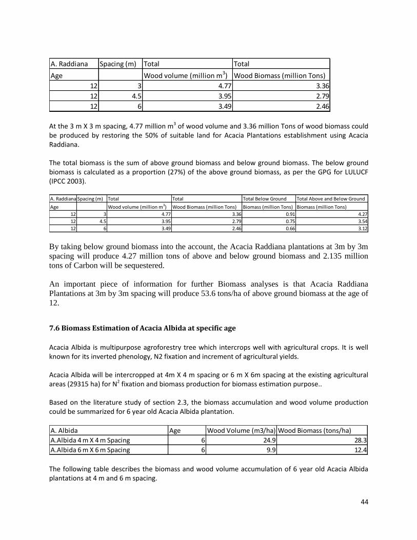
44

At the 3 m X 3 m spacing, 4.77 million m3 of wood volume and 3.36 million Tons of wood biomass could be produced by restoring the 50% of suitable land for Acacia Plantations establishment using Acacia Raddiana. The total biomass is the sum of above ground biomass and below ground biomass. The below ground biomass is calculated as a proportion (27%) of the above ground biomass, as per the GPG for LULUCF (IPCC 2003).

By taking below ground biomass into the account, the Acacia Raddiana plantations at 3m by 3m

spacing will produce 4.27 million tons of above and below ground biomass and 2.135 million

tons of Carbon will be sequestered.

An important piece of information for further Biomass analyses is that Acacia Raddiana

Plantations at 3m by 3m spacing will produce 53.6 tons/ha of above ground biomass at the age of

12.

7.6 Biomass Estimation of Acacia Albida at specific age

Acacia Albida is multipurpose agroforestry tree which intercrops well with agricultural crops. It is well known for its inverted phenology, N2 fixation and increment of agricultural yields. Acacia Albida will be intercropped at 4m X 4 m spacing or 6 m X 6m spacing at the existing agricultural areas (29315 ha) for N2 fixation and biomass production for biomass estimation purpose.. Based on the literature study of section 2.3, the biomass accumulation and wood volume production could be summarized for 6 year old Acacia Albida plantation.

The following table describes the biomass and wood volume accumulation of 6 year old Acacia Albida plantations at 4 m and 6 m spacing.

A. Raddiana Spacing (m) Total Total


12 3 4.77 3.36

12 4.5 3.95 2.79

12 6 3.49 2.46

A. Raddiana Spacing (m) Total Total Total Below Ground Total Above and Below Ground


12 3 4.77 3.36 0.91 4.27

12 4.5 3.95 2.79 0.75 3.54

12 6 3.49 2.46 0.66 3.12

A. Albida Age Wood Volume (m3/ha) Wood Biomass (tons/ha)

A.Albida 4 m X 4 m Spacing 6 24.9 28.3

A.Albida 6 m X 6 m Spacing 6 9.9 12.4

45

At 6 m X 6 m spacing, the Acacia Albida plantations will produce 0.29 million m3 wood volume and 0.36 million tons of wood biomass while providing the space for agriculture crops and providing the N2 fixation service. The total biomass is the sum of above ground biomass and below ground biomass. The below ground biomass is calculated as a proportion (27%) of the above ground biomass, as per the GPG for LULUCF (IPCC 2003).

By taking below ground biomass into the account, the six years old Acacia Albida plantations at

6 m by 6 m spacing will produce 0.46 million tons of above and below ground biomass and 0.23

million tons of Carbon will be sequestered.

An important piece of information for further Biomass analyses is that Acacia Albida Plantations

at 6m by 6m spacing will produce 12.4 tons/ha of above ground biomass at the age of 6.

7.7 Biomass estimation of Acacia Nilotica until 30 years old

An important piece of information from section 7.4 for further Biomass analyses is that Acacia

Nilotica Plantations at 3m by 3m spacing will produce 274.2 tons/ha of above ground biomass at

the age of 30.

IPCC 2003 published Biodiverse Biomass Accumulation (APPENDIX-S) Annex 13(3)

Justification of Yield Data excel sheet which is downloadable from the UNFCCC website. It

illustrated the general trend of biomass increment of trees species for biomass accumulation.

The ratio of Biomass increment from previous year to present year or present year to next year

was calculated based on the Biodiverse Biomass Accumulation. The calculated ratios are

illustrated as the APPENDIX-T.

The annual Biomass accumulation of Acacia Nilotica 274.2 tons at 30 years old plantation was

applied as the reference in order to generate the annual above ground biomass increment in

tons/ha from year 1 to year 30 based on the ratios of Biodiverse Biomass Accumulation.

Age Wood Volume (m3/ha) Wood Biomass (tons/ha) Spacing (m) Trees/Ha Area (Ha) Area (Ha) Area (Ha) Total Total

Waterlogged Agroforestry Acacia Plantations Wood volume (m3) Wood Biomass (Tons)

6 24.9 28.3 4 625.00 0 29314.99 0 729943.251 829614.217

6 9.9 12.4 6 277.78 0 29314.99 0 290218.401 363505.876

A. Albida Spacing (m) Total Total


6 4 0.73 0.83

6 6 0.29 0.36

A. Albida Spacing (m) Total Total Total Below Ground Total Above and Below Ground


6 4 0.73 0.83 0.22 1.05

6 6 0.29 0.36 0.10 0.46

46

The annual below ground biomass increment was derived by 27% of above ground biomass as per the GPG for LULUCF (IPCC 2003).

Then annual total biomass (tons/ha) was calculated by summing the above and below ground

annual values.

The total area for restoration with Acacia Nilotica is 80803.9 ha (18034 ha of potential flooded

zone and 62765.36 ha of suitable Acacia Plantations). The total biomass accumulation was

prorated by multiplying the total restoration area and annual total biomass (tons/ha)

accumulation annually. The annual carbon sequestration was determined as 50% of annual

biomass accumulation as per the IPCC guidelines.

The result for the restoration scenario with Acacia Nilotica was presented as the APPENDIX-U

and illustrated as the following graph.

The total biomass accumulation is 28.14 million tons and total carbon sequestration is 14.07

million tons for the 80803.9 ha of Acacia Nilotica 3m X 3m plantations in the study area at the

biomass accumulation rate of 348.23 tons/ha at the 30 years age of plantation.

7.8 Biomass estimation of Acacia Raddiana until 30 years old

The similar methodological approach was applied to estimate the annual biomass accumulation and

annual carbon sequestration of Acacia Raddiana.

The total area for restoration with Acacia Raddiana is 62765.36 ha (50 % of 125530.72 Ha =

62765.36 ha of suitable Acacia Plantations). The total biomass accumulation was prorated by

47

multiplying the total restoration area and annual total biomass (tons/ha) accumulation annually.

The annual carbon sequestration was determined as 50% of annual biomass accumulation as per

the IPCC guidelines.

The result for the restoration scenario with Acacia Raddiana was presented as the APPENDIX-V

and illustrated as the following graph.

The total biomass accumulation is 15.59 million tons and total carbon sequestration is 7.79

million tons for the 62765.36 ha of Acacia Raddiana at 3m X 3m plantations in the study area at

the biomass accumulation rate of 248.38 tons/ha at the 30 years age of plantation.

7.9 Biomass estimation of Acacia Albida until 30 years old

The similar methodological approach was applied to estimate the annual biomass accumulation and

annual carbon sequestration of Acacia Albida.

The total area for restoration with Acacia Albida is 29314.99 ha of existing agricultural areas.

The total biomass accumulation was prorated by multiplying the total restoration area and annual

total biomass (tons/ha) accumulation annually. The annual carbon sequestration was determined

as 50% of annual biomass accumulation as per the IPCC guidelines.

The result for the restoration scenario with Acacia Raddiana was presented as the APPENDIX-

W and illustrated as the following graph.

48

The total biomass accumulation is 2.83 million tons and total carbon sequestration is 1.42 million

tons for the 29314.99 ha of Acacia Albida at 6m X 6m plantations in the study area at the

biomass accumulation rate of 96.57 tons/ha at the 30 years age of plantation.

This study reviewed the literature in relation to Silvicultural characteristics of Acacia Nilotica,

A. Albida and A. Raddiana for integration with agroforestry and plantation establishment in

order to restore the land.

This study (section 7) estimated the volume, biomass and carbon sequestration capability of

Acacia Nilotica, Acacia Raddiana and Acacia Albida at the specific age based on the published

literature.

This study (section 7) applied the Biodiverse Biomass Accumulation and guidelines of IPCC and

UNFCCC for prorating the annual biomass accumulation and carbon sequestration.

This study (section 7) reports the annual above ground biomass accumulation rate (tons/ha),

annual below ground biomass accumulation rate (tons/ha), annual total biomass accumulation

rate (tons/ha) and annual total carbon sequestration rate (tons/ha) for Acacia Nilotica @ 3m

spacing, A. Raddiana @ 3m spacing and A. Albida @ 6m spacing until 30 years of age

plantations at per hectare basis in Appendix –U, V and W based on the future land use scenario,

Silviculture characteristics and guidelines of IPCC and UNFCCC.

49

References

Badi, K.H, Magid, T.D.A, (2013), Manual of Silviculture for Selected Species in the Sudan, Part-1: Indigenous Species, LAP LAMBERT Academic Publishing Burrough, P.A, McDonnell, R.A, (1998), Principles of Geographical Information Systems, 2nd edition, Oxford University Press Dafa-Alla Mohamed Dafa-Alla, Huda Abdelwahab Shawari and Abdalla Mirghani Eltayeb (2012) “Taungya as a Means of Low-Cost establishment and Sustainable Land use system by, University of Khartoum, Journal of Agricultural Science and Technology”

Gassman, P. W., M. R. Reyes, C. H. Green, and J. G. Arnold (2007), The soil and water assessment tool: Historical development, applications, and future research directions, Trans. ASAE, 50(4), 1211– 1250. J.G. ARNOLD, J.R. KINIRY, R. SRINIVASAN, J.R. WILLIAMS, E.B.HANEY, S.L. NEITSCH, (2011) Soil and Water Assessment Tool, Input / Output Documentation, Version 2009, Texas A&M University Jensen, John R., 2005, Introductory Digital Image Processing, 3rd Ed., Upper Saddle River, NJ: Prentice Hall Jensen, John R., 2007, Remote Sensing of the Environment: An Earth Resource Perspective, 2nd Ed., Upper Saddle River, NJ: Prentice Hall Jurgen Schuol, Karim C. Abbaspou, Hong Yang, Raghavan Srinivasan, and Alexander J. B. Zehnder (2008), Modeling blue water and green water availability in Africa, Water Resource Research, VOL.44, W07406 Jurgen Schuol, Karim C. Abbaspour, Raghavan Srinivasan, Hong Yang (2007), Estimation of freshwater availability in the West African sub-continent using the SWAT hydrologic model, Journal of Hydrology (2008) 352, 30-49 Noy-Meir, I. (1976) "Rotational Grazing in a Continuously Growing Pasture: A Simple Model." Agriculture Systems, 1 87-112 Okorio, J., Maghembe, J.A, (1994), The growth and yield of Acacia albida intercropped with maize (Zea mays) and beans (Phaseolus vulgaris) at Morogoro, Tanzania, Forest Ecology and Management 64 (1994) 183-190 ODUM, EUGENE P, (1983), Basic Ecology, CBS College Publication LILLESAND, T.M & KIEFFER, R.W, Chipman, J., (2007), Remote Sensing and Image Interpretation 6th

Edition, Wiley S.L. NEITSCH, J.G. ARNOLD, J.R. KINIRY, R. SRINIVASAN, J.R. WILLIAMS, (2002), Soil and Water Assessment Tool, User’s Manual, Version 2000, Texas A&M University S.L. NEITSCH, J.G. ARNOLD, J.R. KINIRY, J.R. WILLIAMS, K.W. KING, (2002), Soil and Water Assessment Tool, Theoretical Documentation, Version 2000, Texas A&M University

50

S.L. NEITSCH, J.G. ARNOLD, J.R. KINIRY, J.R. WILLIAMS, (2005), Soil and Water Assessment Tool, Theoretical Documentation, Version 2005, Texas A&M University S.L. NEITSCH, J.G. ARNOLD, J.R. KINIRY, J.R. WILLIAMS, (2010, updated 2011), Soil and Water Assessment Tool, Theoretical Documentation, Version 2009, Texas A&M University S.L. NEITSCH, J.G. ARNOLD, J.R. KINIRY, R. SRINIVASAN, J.R. WILLIAMS, (2004), Soil and Water Assessment Tool, Input / Output Documentation, Version 2005, Texas A&M University TEEB – (2009), The Economics for Ecosystems and Biodiversity for National and International Policy Makers – Summary: Responding to the Value of Nature 2009

Web Reference

http://database.prota.org/PROTAhtml/Acacia%20nilotica_En.htm http://en.wikipedia.org/wiki/Vachellia_tortilis http://www.prota4u.org/protav8.asp?h=M11,M12,M15,M25,M26,M27,M36,M4,M6,M7&t=Acacia,raddiana&p=Acacia+tortilis#Description http://www.prota4u.org/protav8.asp?h=M27&t=Acacia,raddiana&p=Faidherbia+albida#OtherReferences

http://www.hort.purdue.edu/newcrop/duke_energy/Acacia_albida.html http://www.plantzafrica.com/plantefg/faidalb.htm http://www.feedipedia.org/node/357 http://www.allmeasures.com/Formulae/static/materials/113/density.htm http://www.forestoperationsreview.org/news-issues/item/195-understanding-oven-dry-weight http://www.prota4u.org/protav8.asp?h=M4&t=Acacia,raddiana&p=Acacia+tortilis#Synonyms https://www.wageningenur.nl/upload_mm/0/7/0/c1da0b97-5e3f-4bc3-873d-d6ac41cf171b_acatorf.pdf

51

Appendix-A Study Area and its watershed in Zarqa River Basin, Jordan

52

Appendix-B Study Area and its watershed in Al Gadaref State, Sudan

53

Appendix-C Study Area and its watershed near Mopti Region, Mali

54

Appendix-D Present Land Use and Land Cover Map of Study watershed in Jordan

55

Appendix-E Present Land Use and Land Cover Map of Study watershed in Sudan

56

Appendix-F Present Land Use and Land Cover Map of Study watershed in Mali

57

Appendix-G Suitable Areas for Hima Development in the study watershed of Jordan

58

Appendix-H Future Scenario Land use and land cover Map of study watershed in Jordan

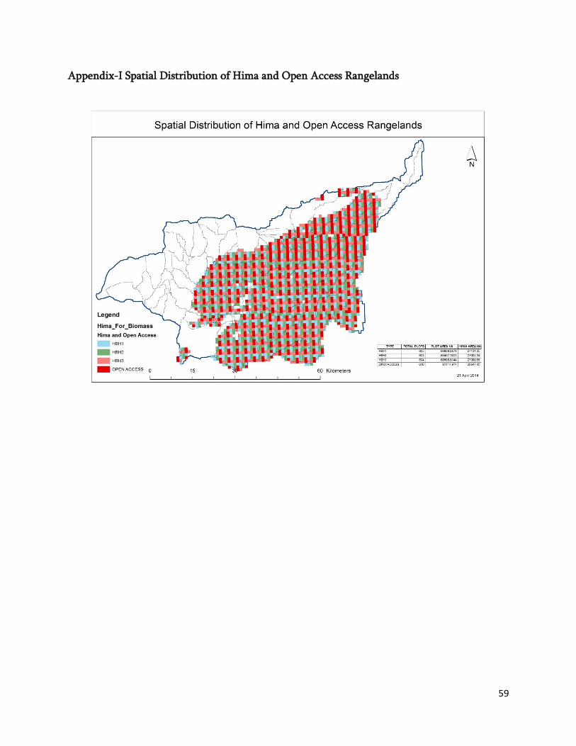
59

Appendix-I Spatial Distribution of Hima and Open Access Rangelands

60

Appendix-J Future Scenario Land Use and Land Cover Map of study watershed in Sudan

61

Appendix-K Future Scenario Land use and land cover Map of study watershed in Mali

62

Appendix-L: Mathematical Formulation of Water Balance

Mathematical formulation of water balance overtime based on the water balance equation is illustrated based on the following diagram m and mathematical derivation.

Mathematically, the following SCS Curve Number equation (1972) has been developed to provide a

consistent basis for estimating the amount of run off under varying land use and soil type. (Rallison and

Miller 1981)

Q = (P-Ia)2/ (P-Ia) + S Although P (precipitation) is known from the weather station, Ia and S are unknown. The Curve Numbers are developed to solve the S (Retention parameter) for various land cover and soil type. (SWAT Theory Document) S = 25.4 [(1000/CN)-10 where CN = Curve Number

Ia is assumed commonly 0.2S for areas except urban areas where Ia is assumed as 0.1S. (SWAT Theory

document) Therefore the (Q) runoff equation in vegetative area and urban or developed area will be as follow.

Q vegetative area = (P-0.2S)2/(P+0.8S) Q Urban or Developed Area = (P-0.1S)2/(P+0.9S) Conceptually, If P=0.2S then Q = 0, meaning that no surface water flow. Conceptually, If P<0.2S then Q will be negative, meaning that meaningless. Therefore the equation is valid for P>=0.2S for vegetative area, otherwise Q will be 0. Similarly in the urban or developed area, the equation is valid for P>=0.1S, otherwise Q will be zero.

63

SWAT Theory document provides the CN values for different land covers and soil types in order to solve the Retention Parameters and Initial abstraction. The following examples are presented from the SWAT Theory document for the reference.

64

65

Appendix-M SWAT Model Parameters for Africa referred by the project

66

APPENDIX-N National Estimates of available water in Africa

67

APPENDIX-O Comparison of results from Published ArcSWAT Africa Study to this project output for Mali

From Attached Paper

Country Area 103 km2 Lower range Blue water flow km3 a-1 Upper range Blue water flow km3 a-1 Lower Ranger Green water flow km3 a-1 Upper Ranger Green water flow km3 a-1

Mali 1256.7 47.7 92.1 267.7 297.8

B.Faso Africa Study 273.7 19 42.5 153.1 173.1

Calculation of M3 Per Ha Actual evapotranspiration

Lower range Blue water flow m3 per Ha Upper range Blue water flow m3 Per Ha Lower Ranger Green water flow m3 Per Ha Upper Ranger Green water flow m3 Per Ha

Mali 379.57 732.87 2130.18 2369.70

B.Faso Africa Study 694.19 1552.80 5593.72 6324.44

Average Mali & B.Faso 536.88 1142.83 3861.95 4347.07

ArcSWAT Sudan Modals

Total Water Yield m3 Per Ha

Present Land use Scenario 646.8 which is within the range of 398 to 967 4228 Evapotranspiration

Future Land Use Scenario 736.6 which is within the range of 398 to 967 4461 Evapotranspiration

Note:

Blue water = Water yield and deep acquifer recharge = Total water yield

Green Water = Actual Evapotranspiration

68

APPENDIX-P Comparison of results from Published ArcSWAT Africa Study to this project output for Sudan

From Attached Paper

Country Area 103 km2 Lower range Blue water flow km3 a-1 Upper range Blue water flow km3 a-1 Lower Ranger Green water flow km3 a-1 Upper Ranger Green water flow km3 a-1

Ethiopia 1132.3 99.1 211.9 627.7 707.2

Sudan 2490.4 45.1 138.3 830.9 930.7

Both Ethiopia and Sudan 3622.7 144.2 350.2 1458.6 1637.9

Calculation of M3 Per Ha Actual evapotranspiration

Lower range Blue water flow m3 per Ha Upper range Blue water flow m3 Per Ha Lower Ranger Green water flow m3 Per Ha Upper Ranger Green water flow m3 Per Ha

Ethiopia 875.21 1871.41 5543.58 6245.69

Sudan 181.10 555.33 3336.41 3737.15

Both Ethiopia and Sudan 398.05 966.68 4026.28 4521.21

ArcSWAT Sudan Modals

Total Water Yield m3 Per Ha

Present Land use Scenario 782 which is within the range of 398 to 967 4770 Evapotranspiration

Future Land Use Scenario 909 which is within the range of 398 to 967 5014 Evapotranspiration

Future Land Use Scenario

with

Increased trees cover 896 which is within the range of 398 to 967 4633 Evapotranspiration

Note:

Blue water = Water yield and deep acquifer recharge = Total water yield

Green Water = Actual Evapotranspiration

69

APPENDIX-Q Summary Statistics based on Sample Data of Bani Hashem Hima Sites

Calculation Based on 95% Confidence Interval

HBH1 HBH2 HBH3 HBH_ALL Open

n - number of samples by Dr. Yahya's Study 20 40 20 80 20

Total Area of study (ha) 19 30 51 100 100

Sample Plot Size (sq m) 1 1 1 1 1

ybar - mean of estimate Fwt.(gr m-1) Fresh Biomass 97.143 73.8955 83.5415 82.1188 8.114

Lower Limit of estimate Fwt.(gr m-1) Fresh Biomass 73.59 55.71775 61.84 70.92 5.46312

Upper Limit of estimate Fwt.(gr m-1) Fresh Biomass 120.695 92.07325 105.2429 93.9 10.76487

Coefficient of variation (%) 51.8 76.92 55.5 64.59 69.81

Margin of Error (%) 24.25 24.59 25.98 14.37 32.67

Standard Error (%) 11.584 8.986 10.368 7.22 15.6091

Recommanded samples n @ 5% Margin of Error 415 909 476 643 751

Recommended Sampling Intensity % @ 5% Margin of Error 0.22 0.3 0.093 0.075 0.075







70

APPENDIX-R Estimating Fresh Biomass to Dry Biomass and Biomass (Kg) Per Ha for Hima

and Open Access rangeland

HBH1 HBH2 HBH3 HBH_ALL Open Remark

Area Ha 19 30 51 100 100

Allowable Dry Yields (Kg) 2557 2735 5715 11007 457

Dry Biomass (Kg)/Ha 134.5789 91.16667 112.0588 110.07 4.57

Dry Biomass (Kg)/sq m 0.013458 0.009117 0.011206 0.011007 0.000457

Dry Biomass (g / sq m) 13.45789 9.116667 11.20588 11.007 0.457

Lower Limit Fresh weight (g/ sq m) 73.57 55.71775 61.84007 70.92178 5.463126

Mean Fresh weight (g/ sq m) 97.143 73.8955 83.5415 82.1188 8.114

Upper Limit Fresh weight (g/ sq m) 120.696 92.07325 105.2429 93.92178 10.76487

Ratio (d/w) for Lower Limit 0.182926 0.163622 0.181207 0.155199 0.083652 Ratio(d/w) for open access is very low

Ratio (d/w) for mean 0.138537 0.123372 0.134136 0.134038 0.056322 So we use the (d/w) ration of HBH

Ratio (d/w) for Upper Limit 0.111502 0.099015 0.106476 0.117193 0.042453 which is statistictically consistant.

Lower Limit Fresh weight (g/ sq m) 73.57 55.71775 61.84007 70.92178 5.463126

Mean Fresh weight (g/ sq m) 97.143 73.8955 83.5415 82.1188 8.114

Upper Limit Fresh weight (g/ sq m) 120.696 92.07325 105.2429 93.92178 10.76487

Lower Limit Fresh weight (kg/ sq m) 0.07357 0.055718 0.06184 0.070922 0.005463

Mean Fresh weight (kg/ sq m) 0.097143 0.073896 0.083542 0.082119 0.008114

Upper Limit Fresh weight (kg/ sq m) 0.120696 0.092073 0.105243 0.093922 0.010765

Lower Limit Fresh weight (kg/ ha) 735.7 557.1775 618.4007 709.2178 54.63126

Mean Fresh weight (kg/ ha) 971.43 738.955 835.415 821.188 81.14

Upper Limit Fresh weight (kg/ ha) 1206.96 920.7325 1052.429 939.2178 107.6487

New estimate for Open Access

Lower Limit Dry weight (kg/ ha) 134.5789 91.16667 112.0588 110.07 4.57 8.478725137

Mean Dry weight (kg/ ha) 134.5789 91.16667 112.0588 110.07 4.57 10.87580408

Upper Limit dry weight (kg/ ha) 134.5789 91.16667 112.0588 110.07 4.57 12.61570257

Lower Limit Dry weight (kg/ ha) 114.18 86.47347 95.97526 110.07 8.478725

Mean Dry weight (kg/ ha) 130.2081 99.04769 111.977 110.07 10.8758

Upper Limit dry weight (kg/ ha) 141.4476 107.9036 123.3376 110.07 12.6157

Lower Limit Dry weight (kg/ ha) 98.87625 8.478725

Mean Dry weight (kg/ ha) 113.7442 Final Estimate for Hima 10.8758 Final estimate for Open Access

Upper Limit dry weight (kg/ ha) 124.2296 12.6157

71

APPENDIX-S Biodiverse Biomass Accumulation from cdm.unfccc.int

Biodiverse Biomass accumulation tons dry mass / ha (t.d.m/ha)

Above

ground

biomass

Below

ground

biomass

Total

biomass

t d.m./ha t d.m./ha t d.m./ha

1 1.9 0.5 2.5

2 5.1 1.4 6.5 Parameters used Value Unit Source

3 8.8 2.4 11.1 Root to shoot 0.27 dimensionless Table 3A.1.8 GPG IPCC 2003

4 13.1 3.6 16.7 Carbon Fraction 0.5 tC/t d.m. IPCC

5 18.0 4.9 22.9

6 23.4 6.3 29.7

7 29.2 7.9 37.1

8 35.6 9.6 45.2

9 42.4 11.4 53.8

10 49.9 13.5 63.4

11 57.5 15.5 73.0

12 39.3 10.6 49.9

13 46.8 12.6 59.5

14 54.6 14.7 69.4

15 62.2 16.8 79.0

16 69.5 18.8 88.2

17 76.5 20.7 97.2

18 83.6 22.6 106.2

19 90.7 24.5 115.1

20 97.7 26.4 124.1

21 104.8 28.3 133.1

22 86.9 23.5 110.3

23 93.9 25.4 119.3

24 101.0 27.3 128.2

25 108.0 29.2 137.2

26 115.1 31.1 146.2

27 122.2 33.0 155.1

28 129.2 34.9 164.1

29 136.3 36.8 173.1

30 143.3 38.7 182.1

Age

72

APPENDIX –T: Ratios of biomass increment based on Biodiverse Biomass Accumulation

Above

ground

biomass

Below

ground

biomass

Total

biomass

Ratio of

Above Ground Biomass to the

previous,

present and next year(fraction)

t d.m./ha t d.m./ha t d.m./ha Fraction

1 1.9 0.5 2.5

2 5.1 1.4 6.5 2.6

3 8.8 2.4 11.1 1.7

4 13.1 3.6 16.7 1.5

5 18.0 4.9 22.9 1.4

6 23.4 6.3 29.7 1.3

7 29.2 7.9 37.1 1.3

8 35.6 9.6 45.2 1.2

9 42.4 11.4 53.8 1.2

10 49.9 13.5 63.4 1.2

11 57.5 15.5 73.0 1.2

12 39.3 10.6 49.9 0.7

13 46.8 12.6 59.5 1.2

14 54.6 14.7 69.4 1.2

15 62.2 16.8 79.0 1.1

16 69.5 18.8 88.2 1.1

17 76.5 20.7 97.2 1.1

18 83.6 22.6 106.2 1.1

19 90.7 24.5 115.1 1.1

20 97.7 26.4 124.1 1.1

21 104.8 28.3 133.1 1.1

22 86.9 23.5 110.3 0.8

23 93.9 25.4 119.3 1.1

24 101.0 27.3 128.2 1.1

25 108.0 29.2 137.2 1.1

26 115.1 31.1 146.2 1.1

27 122.2 33.0 155.1 1.1

28 129.2 34.9 164.1 1.1

29 136.3 36.8 173.1 1.1

30 143.3 38.7 182.1 1.1

Age

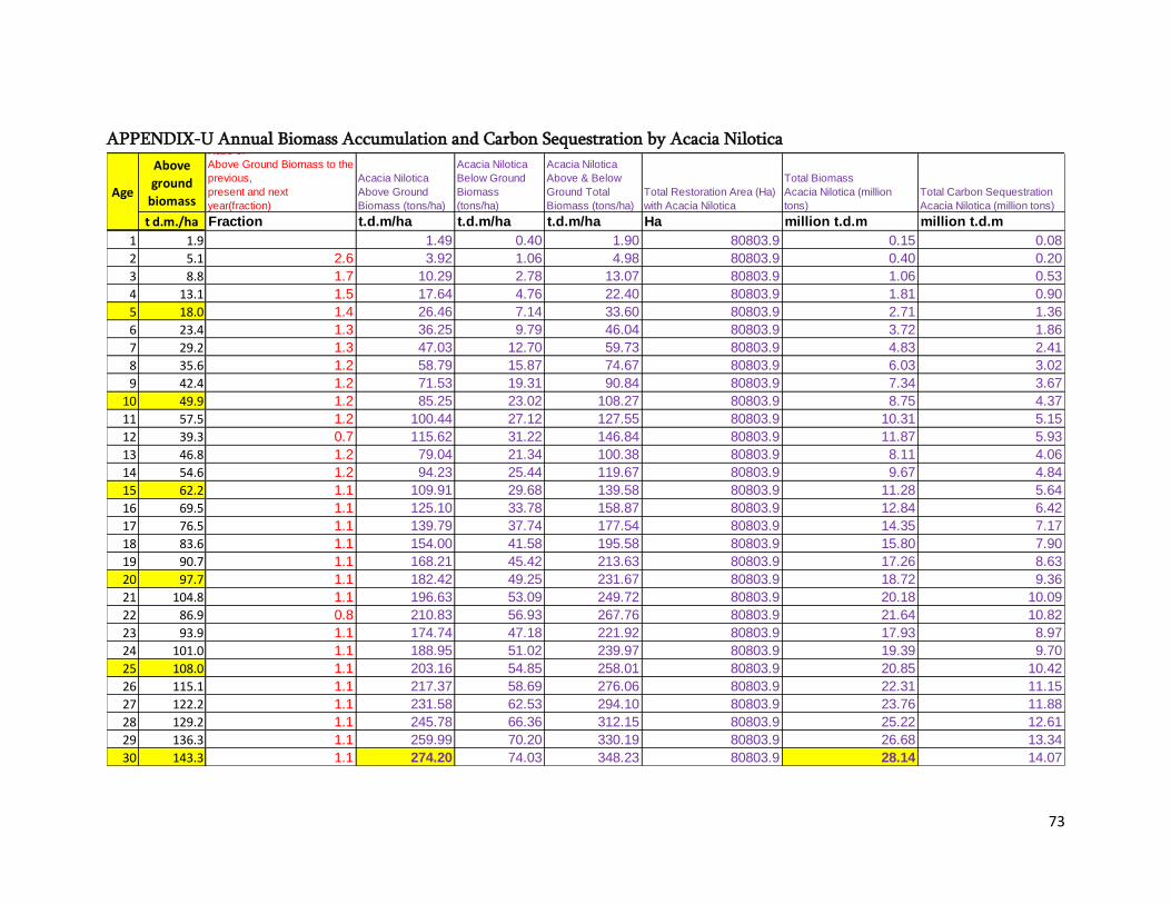
73

APPENDIX-U Annual Biomass Accumulation and Carbon Sequestration by Acacia Nilotica

Above

ground

biomass

Ratio of


previous,

present and next

year(fraction)

Acacia Nilotica

Above Ground

Biomass (tons/ha)

Acacia Nilotica

Below Ground

Biomass

(tons/ha)

Acacia Nilotica

Above & Below

Ground Total

Biomass (tons/ha)

Total Restoration Area (Ha)

with Acacia Nilotica

Total Biomass

Acacia Nilotica (million

tons)

Total Carbon Sequestration

Acacia Nilotica (million tons)

t d.m./ha Fraction t.d.m/ha t.d.m/ha t.d.m/ha Ha million t.d.m million t.d.m

1 1.9 1.49 0.40 1.90 80803.9 0.15 0.08

2 5.1 2.6 3.92 1.06 4.98 80803.9 0.40 0.20

3 8.8 1.7 10.29 2.78 13.07 80803.9 1.06 0.53

4 13.1 1.5 17.64 4.76 22.40 80803.9 1.81 0.90

5 18.0 1.4 26.46 7.14 33.60 80803.9 2.71 1.36

6 23.4 1.3 36.25 9.79 46.04 80803.9 3.72 1.86

7 29.2 1.3 47.03 12.70 59.73 80803.9 4.83 2.41

8 35.6 1.2 58.79 15.87 74.67 80803.9 6.03 3.02

9 42.4 1.2 71.53 19.31 90.84 80803.9 7.34 3.67

10 49.9 1.2 85.25 23.02 108.27 80803.9 8.75 4.37

11 57.5 1.2 100.44 27.12 127.55 80803.9 10.31 5.15

12 39.3 0.7 115.62 31.22 146.84 80803.9 11.87 5.93

13 46.8 1.2 79.04 21.34 100.38 80803.9 8.11 4.06

14 54.6 1.2 94.23 25.44 119.67 80803.9 9.67 4.84

15 62.2 1.1 109.91 29.68 139.58 80803.9 11.28 5.64

16 69.5 1.1 125.10 33.78 158.87 80803.9 12.84 6.42

17 76.5 1.1 139.79 37.74 177.54 80803.9 14.35 7.17

18 83.6 1.1 154.00 41.58 195.58 80803.9 15.80 7.90

19 90.7 1.1 168.21 45.42 213.63 80803.9 17.26 8.63

20 97.7 1.1 182.42 49.25 231.67 80803.9 18.72 9.36

21 104.8 1.1 196.63 53.09 249.72 80803.9 20.18 10.09

22 86.9 0.8 210.83 56.93 267.76 80803.9 21.64 10.82

23 93.9 1.1 174.74 47.18 221.92 80803.9 17.93 8.97

24 101.0 1.1 188.95 51.02 239.97 80803.9 19.39 9.70

25 108.0 1.1 203.16 54.85 258.01 80803.9 20.85 10.42

26 115.1 1.1 217.37 58.69 276.06 80803.9 22.31 11.15

27 122.2 1.1 231.58 62.53 294.10 80803.9 23.76 11.88

28 129.2 1.1 245.78 66.36 312.15 80803.9 25.22 12.61

29 136.3 1.1 259.99 70.20 330.19 80803.9 26.68 13.34

30 143.3 1.1 274.20 74.03 348.23 80803.9 28.14 14.07

Age

74

APPENDIX-V Annual Biomass Accumulation and Carbon Sequestration by Acacia Raddiana

Above

ground

biomass

Ratio of


previous,


Acacia Raddiana

Above Ground

Biomass (tons/ha)

Acacia Raddiana

Below Ground

Biomass (tons/ha)

Acacia Raddiana

Above & Below

Ground Total

Biomass (tons/ha)

Total Restoration Area

(Ha)

with Acacia Raddiana

Total Biomass

Acacia Raddiana (million

tons)

Total Carbon Sequestraion

Acacia Raddiana (million

tons)


1 1.9 0.69 0.19 0.88 62765.36 0.06 0.03

2 5.1 2.6 1.82 0.49 2.31 62765.36 0.14 0.07

3 8.8 1.7 4.77 1.29 6.06 62765.36 0.38 0.19

4 13.1 1.5 8.18 2.21 10.38 62765.36 0.65 0.33

5 18.0 1.4 12.26 3.31 15.58 62765.36 0.98 0.49

6 23.4 1.3 16.81 4.54 21.34 62765.36 1.34 0.67

7 29.2 1.3 21.80 5.89 27.69 62765.36 1.74 0.87

8 35.6 1.2 27.25 7.36 34.61 62765.36 2.17 1.09

9 42.4 1.2 33.16 8.95 42.11 62765.36 2.64 1.32

10 49.9 1.2 39.52 10.67 50.19 62765.36 3.15 1.58

11 57.5 1.2 46.56 12.57 59.13 62765.36 3.71 1.86

12 39.3 0.7 53.60 14.47 68.07 62765.36 4.27 2.14

13 46.8 1.2 63.90 17.25 81.15 62765.36 5.09 2.55

14 54.6 1.2 74.53 20.12 94.65 62765.36 5.94 2.97

15 62.2 1.1 84.83 22.90 107.73 62765.36 6.76 3.38

16 69.5 1.1 94.80 25.60 120.39 62765.36 7.56 3.78

17 76.5 1.1 104.43 28.20 132.63 62765.36 8.32 4.16

18 83.6 1.1 114.07 30.80 144.86 62765.36 9.09 4.55

19 90.7 1.1 123.70 33.40 157.10 62765.36 9.86 4.93

20 97.7 1.1 133.33 36.00 169.34 62765.36 10.63 5.31

21 104.8 1.1 142.97 38.60 181.57 62765.36 11.40 5.70

22 86.9 0.8 118.50 31.99 150.49 62765.36 9.45 4.72

23 93.9 1.1 128.13 34.60 162.73 62765.36 10.21 5.11

24 101.0 1.1 137.77 37.20 174.96 62765.36 10.98 5.49

25 108.0 1.1 147.40 39.80 187.20 62765.36 11.75 5.87

26 115.1 1.1 157.03 42.40 199.43 62765.36 12.52 6.26

27 122.2 1.1 166.67 45.00 211.67 62765.36 13.29 6.64

28 129.2 1.1 176.30 47.60 223.91 62765.36 14.05 7.03

29 136.3 1.1 185.94 50.20 236.14 62765.36 14.82 7.41

30 143.3 1.1 195.57 52.80 248.38 62765.36 15.59 7.79

Age

75

APPENDIX-W Annual Biomass Accumulation and Carbon Sequestration by Acacia Albida

Above

ground

biomass

Ratio of


previous,


Acacia Albida

Above Ground Biomass

(tons/ha)

Acacia Albida

Below Ground

Biomass (tons/ha)

Acacia Albida

Above & Below

Ground Total

Biomass (tons/ha)

Total Restoration Area (Ha)

with Acacia Albida

Total Biomass

Acacia Albida (million tons)

Total Carbon

Sequestration

Acacia Albida (million tons)


1 1.9 0.51 0.14 0.65 29314.99 0.02 0.01

2 5.1 2.6 1.34 0.36 1.70 29314.99 0.05 0.02

3 8.8 1.7 3.52 0.95 4.47 29314.99 0.13 0.07

4 13.1 1.5 6.03 1.63 7.66 29314.99 0.22 0.11

5 18.0 1.4 9.05 2.44 11.49 29314.99 0.34 0.17

6 23.4 1.3 12.40 3.35 15.75 29314.99 0.46 0.23

7 29.2 1.3 15.50 4.19 19.69 29314.99 0.58 0.29

8 35.6 1.2 18.86 5.09 23.95 29314.99 0.70 0.35

9 42.4 1.2 22.48 6.07 28.54 29314.99 0.84 0.42

10 49.9 1.2 26.48 7.15 33.63 29314.99 0.99 0.49

11 57.5 1.2 30.48 8.23 38.71 29314.99 1.13 0.57

12 39.3 0.7 20.84 5.63 26.47 29314.99 0.78 0.39

13 46.8 1.2 24.84 6.71 31.55 29314.99 0.92 0.46

14 54.6 1.2 28.98 7.82 36.80 29314.99 1.08 0.54

15 62.2 1.1 32.98 8.90 41.89 29314.99 1.23 0.61

16 69.5 1.1 36.86 9.95 46.81 29314.99 1.37 0.69

17 76.5 1.1 40.60 10.96 51.56 29314.99 1.51 0.76

18 83.6 1.1 44.35 11.97 56.32 29314.99 1.65 0.83

19 90.7 1.1 48.09 12.99 61.08 29314.99 1.79 0.90

20 97.7 1.1 51.84 14.00 65.84 29314.99 1.93 0.96

21 104.8 1.1 55.58 15.01 70.59 29314.99 2.07 1.03

22 86.9 0.8 46.07 12.44 58.51 29314.99 1.72 0.86

23 93.9 1.1 49.82 13.45 63.27 29314.99 1.85 0.93

24 101.0 1.1 53.56 14.46 68.02 29314.99 1.99 1.00

25 108.0 1.1 57.31 15.47 72.78 29314.99 2.13 1.07

26 115.1 1.1 61.05 16.48 77.54 29314.99 2.27 1.14

27 122.2 1.1 64.80 17.50 82.29 29314.99 2.41 1.21

28 129.2 1.1 68.54 18.51 87.05 29314.99 2.55 1.28

29 136.3 1.1 72.29 19.52 91.81 29314.99 2.69 1.35

30 143.3 1.1 76.04 20.53 96.57 29314.99 2.83 1.42

Age

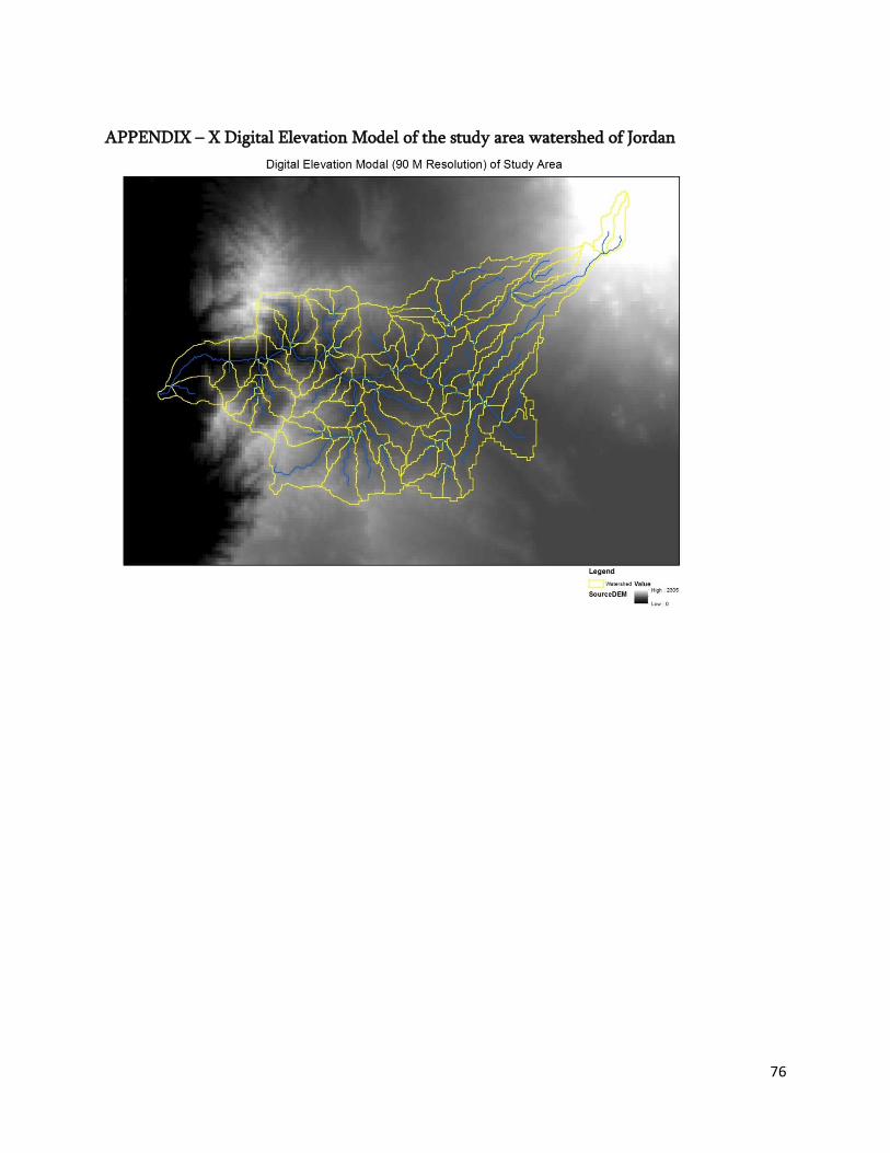
76

APPENDIX – X Digital Elevation Model of the study area watershed of Jordan

77

APPENDIX – Y Digital Elevation Model of the study area watershed of Sudan

78

APPENDIX-Z Digital Elevation Model of the study area watershed of Mali

79

APPENDIX – AA FAO Soil Map of the study area watershed of Jordan

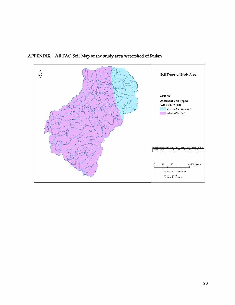
80

APPENDIX – AB FAO Soil Map of the study area watershed of Sudan

81

APPENDIX – AC FAO Soil Map of the study area watershed of Mali

82

APPENDIX-AD Daily Weather data description for the study areas of Jordan, Sudan and

Mali

Daily weather Data for Study area of Jordan www.glodalweather.tamu.edu Climate Data South Latitude: 28.78 West Longitude: 34.5 North Latitude: 33.21 East Longitude: 39.5 Number of Weather Stations: 224 Start Date: 12/1/1990 End Date: 12/31/2010 Starting Hour of Day: 12:00 AM Data Collected: Temperature (C) Precipitation (mm) Wind (m/s) Relative Humidity (fraction) Solar (MJ/m^2)

Daily weather Data for Study area of Sudan www.glodalweather.tamu.edu Climate Data South Latitude: 12.5 West Longitude: 33.5 North Latitude: 15.5 East Longitude: 36.5 Number of Weather Stations: 90 Start Date: 12/1/1990 End Date: 12/31/2010 Starting Hour of Day: 12:00 AM Data Collected: Temperature (C) Precipitation (mm) Wind (m/s) Relative Humidity (fraction) Solar (MJ/m^2)

Daily weather Data for Study area of Mali www.glodalweather.tamu.edu Climate Data South Latitude: 12.5 West Longitude: 33.5 North Latitude: 15.5 East Longitude: 36.5 Number of Weather Stations: 90 Start Date: 12/1/1990 End Date: 12/31/2010 Starting Hour of Day: 12:00 AM Data Collected: Temperature (C) Precipitation (mm) Wind (m/s) Relative Humidity (fraction) Solar (MJ/m^2)

83

APPENDIX – AE Monthly Weather Data of Mopti Weather Station for the Study Area of

Mali

MOPTI

PLUVIOMETRIE MENSUELLE ( mm )

Année Jan Fév Mar Avr Mai Jui Jui Août Sep Oct Nov Déc TOTAL

2000 0.0 0.0 1.0 0.6 80.7 28.8 86.8 138.5 77.1 0.0 0.0 0.0 413.5

2001 0.0 0.0 0.0 0.0 22.9 89.6 175.5 153.0 70.8 11.7 0.0 0.0 523.5

2002 0.0 0.0 0.0 0.5 12.2 13.4 38.9 77.5 41.7 58.1 0.0 0.1 242.4

2003 0.0 0.0 0.5 0.0 15.0 131.0 221.1 166.7 75.7 9.0 2.8 0.0 621.8

2004 0.5 0.0 0.0 2.7 0.9 51.5 143.0 207.3 37.9 12.7 0.0 0.0 456.5

2005 0.0 0.0 0.0 0.0 13.0 41.2 118.2 123.9 81.4 11.8 0.0 0.0 389.5

2006 0.0 0.0 0.0 0.0 7.9 17.2 152.3 189.9 88.8 3.4 0.0 0.0 459.5

2007 0.0 0.0 0.3 1.0 9.4 52.7 192.0 200.8 101.2 0.0 0.0 0.0 557.4

2008 0.0 0.0 0.0 18.9 58.4 97.7 147.4 213.5 69.0 17.0 0.0 0.0 621.9

2009 0.0 0.3 8.0 0.0 11.5 17.0 112.5 233.6 141.3 58.7 2.3 0.0 585.2

2010 0.0 0.0 0.0 13.1 16.1 139.9 131.4 278.5 226.5 4.6 0.0 0.0 810.1

2011 0.0 0.0 0.0 0.0 8.6 101.3 105.1 175.0 117.6 2.2 0.0 0.0 509.8

MOPTI

TEMPERATURE MAXIMUM MENSUELLE ( °C )

Année Jan Fév Mar Avr Mai Jui Jui Août Sep Oct Nov Déc MOY

2000 34.6 33.8 38.6 43.1 40.4 38.8 35.5 29.3 28.2 36.8 36.7 33.2 35.8

2001 34.1 35.0 40.6 41.4 42.1 37.5 34.9 33.1 33.7 37.5 37.1 35.4 36.9

2002 32.3 35.0 39.9 41.2 42.0 39.8 37.6 34.6 37.1 37.3 37.2 33.9 37.3

2003 31.3 37.7 39.3 42.5 41.6 36.9 33.4 31.7 33.1 36.7 36.3 32.6 36.1

2004 31.8 36.3 37.8 40.5 42.4 39.0 34.0 33.8 35.4 38.2 36.4 35.3 36.7

2005 30.8 35.4 39.5 42.1 40.9 37.9 34.1 33.1 34.4 37.7 37.3 34.3 36.5

2006 31.8 34.6 39.4 41.3 41.2 39.5 36.7 32.8 34.0 36.3 36.7 31.7 36.3

2007 32.4 35.7 39.1 41.5 41.9 38.7 34.6 32.1 33.7 36.4 36.1 33.7 36.3

2008 29.5 36.0 39.6 40.4 41.1 38.6 35.2 32.4 33.3 34.9 35.6 32.7 35.8

2009 29.6 36.5 39.6 41.0 41.8 39.5 36.5 33.9 33.5 35.7 34.5 34.8 36.4

2010 34.5 38.9 39.9 41.7 42.4 38.4 35.9 32.9 33.2 35.7 36.5 35.5 37.1

2011 33.8 34.0 40.6 40.9 41.5 38.6 35.5 33.8 34.9 33.8 38.0 32.3 36.5

MOPTI

TEMPERATURE MINIMUM MENSUELLE ( °C )

Années Jan Fév Mar Avr Mai Jui Jui Août Sep Oct Nov Déc MOY

2000 18.8 16.0 21.0 26.2 26.2 26.1 24.5 23.6 24.5 24.0 19.8 15.1 22.2

2001 14.1 16.3 21.5 24.5 27.5 24.2 23.1 23.5 24.3 23.0 19.9 18.2 21.7

2002 16.4 16.7 22.9 26.1 28.3 26.9 25.1 23.8 25.2 24.5 21.4 17.7 22.9

2003 15.3 20.7 22.6 26.5 27.8 25.8 23.5 23.2 24.7 24.3 21.4 15.7 22.6

2004 16.2 19.3 22.2 26.7 27.4 26.9 23.7 23.6 24.2 24.0 21.2 19.3 22.9

2005 16.6 22.0 24.5 25.4 27.6 26.9 24.3 23.8 24.6 24.2 19.9 17.9 23.1

2006 16.1 18.3 21.8 26.7 26.8 26.9 25.0 23.8 24.3 24.7 20.6 15.2 22.5

2007 15.1 17.2 21.9 27.1 27.8 26.3 24.0 23.6 24.5 24.0 20.7 16.9 22.4

2008 12.3 18.0 22.0 23.9 27.1 25.9 24.0 23.5 24.3 24.4 19.1 16.1 21.7

2009 14.1 20.0 24.4 25.7 27.3 27.1 25.1 23.6 23.8 23.9 19.4 16.8 22.6

2010 15.3 20.3 23.4 27.7 29.0 26.8 25.2 23.6 23.5 24.2 20.7 15.8 23.0

2011 15.5 17.2 24.3 24.6 27.9 26.1 25.0 23.6 23.8 24.1 19.3 13.8 22.1

M O P T I

HUMIDITE RELATIVE MAXIMUM ( % )


2000 46 30 29 37 63 68 82 90 83 67 48 47 58

2001 38 28 27 29 53 78 88 93 86 72 55 42 57

2002 34 29 26 32 48 63 75 87 80 74 53 56 55

2003 40 25 25 35 51 76 89 93 86 75 69 52 60

2004 47 34 31 43 46 69 87 91 88 68 56 49 59

2005 34 34 34 30 52 71 88 91 92 76 53 44 58

2006 38 38 26 39 46 63 73 90 89 79 54 49 57

2007 42 39 33 43 49 64 88 93 92 81 56 49 61

2008 55 42 33 40 58 72 88 91 93 89 66 56 65

2009 54 43 46 37 56 68 82 93 95 90 71 59 66

2010 48 46 31 48 62 76 84 95 97 91 75 68 68

2011 53 39 40 42 57 77 84 93 92 76 56 48 63

84

M O P T I

HUMIDITE RELATIVE MINIMUM ( % )


2000 14 5 6 10 24 30 42 48 42 28 12 9 23

2001 5 5 9 9 18 35 47 56 46 26 12 12 23

2002 8 8 5 12 19 25 38 47 37 30 13 12 21

2003 11 6 5 11 19 35 52 60 47 31 13 13 25

2004 12 7 7 15 13 28 46 52 42 21 13 12 22

2005 9 12 10 5 19 32 48 55 49 26 10 12 24

2006 11 10 4 14 16 25 39 56 52 36 12 16 24

2007 12 11 12 15 18 27 48 62 56 36 16 16 27

2008 19 17 11 12 19 30 44 55 54 43 13 15 28

2009 18 13 13 10 19 28 40 54 58 40 19 12 27

2010 9 10 7 17 31 36 45 61 64 45 21 10 30

2011 10 12 11 12 19 32 45 54 51 26 10 10 24

MOPTI

VENT MOYEN MENSUEL ( m/s )

Année Jan Fév Mar Avr Mai Jui Jui Août Sep Oct Nov Déc MOY

2000 2.5 3.0 2.5 3.0 3.0 3.4 2.8 2.0 1.9 1.8 1.8 2.5 2.5

2001 2.6 3.1 3.4 3.7 4.1 4.4 4.8 3.7 3.8 1.2 2.0 2.2 3.3

2002 2.6 3.8 4.2 3.5 4.3 4.1 4.2 3.1 2.0 1.7 2.6 2.9 3.3

2003 2.9 2.8 3.8 3.6 3.3 4.2 3.7 3.5 3.1 2.7 2.0 2.3 3.2

2004 3.6 4.5 3.0 2.8 4.2 4.0 3.6 3.2 2.8 2.2 2.2 3.3 3.3

2005 4.0 4.4 3.9 3.0 3.3 4.3 4.1 3.3 2.6 2.3 2.1 3.3 3.5

2006 3.2 3.4 3.5 2.8 3.1 4.7 4.0 2.4 2.1 2.1 3.1 3.0 3.1

2007 2.8 2.9 3.1 3.3 3.1 3.1 3.4 2.8 2.8 2.5 3.2 3.5 3.0

2008 2.9 3.7 3.4 3.7 3.5 4.5 4.1 3.2 2.7 2.6 3.3 3.1 3.4

2009 3.0 3.5 3.4 3.3 3.5 4.1 3.9 3.0 2.6 2.1 2.5 2.9 3.2

2010 3.1 3.5 3.9 3.3 3.6 4.0 3.3 2.4 2.0 2.3 2.5 2.5 3.0

2011 3.3 4.2 3.1 3.1 3.3 3.8 3.5 2.7 2.7 2.3 2.6 3.3 3.2

MOPTI

DUREE DE L' ENSOLEILLEMENT ( hours )

Année Jan Fév Mar Avr Mai Jui Jui Août Sep Oct Nov Déc TOTAL

2000 274.8 284.3 284.6 ** ** ** ** ** ** 295.7 276.6 ** **

2001 ** ** ** ** ** ** ** ** ** ** 291.7 286.7 **

2002 261.6 ** 260.4 ** ** 228.3 ** ** ** ** ** ** **

2003 ** ** ** ** ** ** ** ** ** ** 265.6 281.0 **

2004 ** ** ** ** ** ** ** ** ** ** ** ** **

2005 ** ** ** ** ** ** ** ** ** ** ** ** **

2006 ** ** ** ** ** ** ** ** ** ** ** ** **

2007 ** ** ** 242.8 ** ** ** 247.8 ** ** 269.2 ** **

2008 308.9 288.4 315.3 290.1 282.3 256.5 283.3 ** 243.8 268.7 303.7 289.5 **

2009

2010 299.3 280.2 238.3 167.3 208.3 206.5 199.5 228.8 225.6 266.5 248.8 302.7 2871.8

2011 279.3 278.4 260.0 231.5 213.7 213.9 250.1 242.3 256.3 277.6 301.7 288.3 3093.1

EVAPOTRANSPIRATION POTENTIELLE MOYENNE 1981-1990 (ETP mensuelle en mm)

MOPTI

JANV. FEV. MARS AVRIL MAI JUIN JUIL. AOUT SEPT. OCT. NOV. DEC. TOTAL

142 156 216 211 206 186 166 160 146 147 141 126 2003

Documents

Biophysical Analyses Final Report For Study the changes to ... · Biophysical Analyses Final ... APPENDIX-Q Summary Statistics based on Sample Data of Bani Hashem ... Ms. Samia Bakheit