Embed Size (px)
Citation preview

BiomechanicsConcepts and Computation
Answers to the Exercises
Version 3.0
Cees OomensMarcel Brekelmans
Oktober 2011
Eindhoven University of Technology
Department of Biomedical Engineering
Tissue Biomechanics & Engineering
Contents
1 Answers to the exercises of chapter 1 page 1
2 Answers to the exercises of chapter 2 4
3 Answers to the exercises of chapter 3 5
4 Answers to the exercises of chapter 4 7
5 Answers to the exercises of chapter 5 9
6 Answers to the exercises of chapter 6 15
7 Answers to the exercises of chapter 7 18
8 Answers to the exercises of chapter 8 20
9 Answers to the exercises of chapter 9 22
10 Answers to the exercises of chapter 10 23
11 Answers to the exercises of chapter 11 25
12 Answers to the exercises of chapter 12 26
13 Answers to the exercises of chapter 13 27
14 Answers to the exercises of chapter 14 29
15 Answers to the exercises of chapter 15 38
16 Answers to the exercises of chapter 16 41
17 Answers to the exercises of chapter 17 48
18 Answers to the exercises of chapter 18 51
ii

1
Answers to the exercises of chapter 1
Exercises
1.1 (a) |~ei| = 1
(b) ~ei · ~ej = 0 if i 6= j
~ei · ~ej = 1 if i = j
(c) ~ex · (~ey × ~ez) = 1
(d) Definition of a right-handed orthonormal basis.
1.2 ~F z = ~ex − 3~ey − 5~ez
1.3 (a)
a∼=
0
0
4
b∼=
0
−3
4
c∼=
1
0
2
(b)
~a+~b = −3~ey + 8~ez
3(~a+~b+ ~c) = 3~ex − 9~ey + 30~ez
(c)
~a ·~b = ~b · ~a = 16
~a×~b = 12~ex~b× ~a = −12~ex
(d)
|~a| = 4
|~b| = 5
1

2 Answers to the exercises of chapter 1
|~a×~b| = 12
|~b× ~a| = 12
(e) φ = arccos( 45 )
(f) ~ex or −~ex(g)
~a×~b · ~c = 12
~a× ~c ·~b = −12
(h)
~a~b · ~c = 32~ez
(~a~b)T · ~c = −24~ey + 32~ez~b~a · ~c = −24~ey + 32~ez
(i) The vectors are independent, but not perpendicular. So the
vectors ~a, ~b and ~c form a suitable but non-orthogonal basis.
1.4
~d+ ~e = 3~a+ 2~b− 3~c
~d · ~e = 24
1.5 (a) ~az = −25~ez(b) |~ax| = |~ay| = 5 ; |~az| = 25
(c) ~ax × ~ay · ~az = 625
(d) φ = π2
(e)
~αx = 4/5 ~ex + 3/5 ~ey
~αy = 3/5 ~ex − 4/5 ~ey
~αz = −~ez
So the basis {~αx, ~αy, ~αz} is right-handed and orthogonal.
(f)
~b = 2~ex + 3~ey + ~ez
so with respect to {~ex, ~ey, ~ez}, b∼= [ 2 3 1 ]T

Exercises 3
~b =17
25~ax −
6
25~ay −
1
25~az
so with respect to {~ax,~ay,~az}, b∼=1
25[ 17 − 6 − 1 ]T
~b =17
5~αx −
6
5~αy − ~αz
so with respect to {~αx, ~αy, ~αz}, b∼=1
5[ 17 − 6 − 1 ]T
1.6 The triple product is zero. This means that the vectors are not
independent. The vector ~a is lying in the plane, that is defined
by the vectors ~b and ~c. Relation: 2~a−~b− ~c = ~0.
1.7 Both operators are associated with a rotation.
1.8 (a) ax~ex(b) ax~ex + ay~ey(c) no effect
(d) ay~ex − ax~ey + az~ez(e) ax~ex − ay~ey + az~ez

2
Answers to the exercises of chapter 2
Exercises
2.1 (a) ~F = 52
√2 ~ε1 + 1
2
√2 ~ε2 − 4 ~ε3
(b) |~F | =√
29
2.2 (a) ~MP = ~0 ; ~MR = −2 ~ez(b) M∼P = [ 0 0 0 ]T ; M∼R = [ 0 0 − 2 ]T
2.3 (a) 0
(b) 2F` positive if counterclockwise
(c) F` positive if counterclockwise
(d) 2F` positive if counterclockwise
(e) 2F` positive if counterclockwise
2.4 f = Rr F
2.5 ~MP = 6~ex − 9~ey
2.6 ~MS = 12~ez ; ~ME = 3~ez
2.7 (a) ~MS = 3~ey + 3~ez(b) ~MO = −2~ex + 22~ey + 13~ez
4

3
Answers to the exercises of chapter 3
Exercises3.1
~MP = −6~ez ; ~MR = −6~ez
3.2 Define the reaction force vector at A as ~FA and the moment
vector ~MA. For both constructions: FAx = −F ;FAy = 0;
FAz = 0;MAx = 0;MAy = −bF ;MAz = cF .
3.3 For the direction of the forces see the figure below.
va
f
pvb
a
l2
l
VA = (1− α
`)F +
P
2
VB =α
`F +
P
2
5

6 Answers to the exercises of chapter 3
3.4 For the direction of the forces see the next figure.
vc
a
G vb
b
VB =G(a+ b)
a; VC = −Gb
a
3.5 Problem at the left:
For the direction of the forces see the figure below.
va
ha
G
hb
HA =G cos(α)
2 sin(α); VA = G ; HB =
G cos(α)
2 sin(α)
Problem at the right:
For the direction of the forces see the following figure.
va
G
hb
vb
VA =1
2G ; HB = 0 ; VB =
1
2G

4
Answers to the exercises of chapter 4
Exercises4.1 (a)
F = cδ
`c+ c
(`0`c− 1
)(b)
F = c
(`0`c− 1
)4.2 See the graph below.
lc lo lc2 lo2
c
F
4.3 (a) The number of cross bridges that are able to make a connec-
tion is decreasing.
(b) c ≈ 220 [N]
7

8 Answers to the exercises of chapter 4
4.4
δ =
(`mccm
+`t0ct
)F + `mc − `m0
4.5
~FB = −~FA = 160~ex − 120~ey
4.6
~F = c
(√L2 +R2 + 2RL sin(φ)√
L2 +R2− 1
)R cos(φ)~ex − (R sin(φ) + L)~ey√
L2 +R2 + 2RL sin(φ)

5
Answers to the exercises of chapter 5
Exercises5.1 (a)
τF + F = cε with τ =cηc
(b)
F = c e−t/τ
0 0.2 0.4 0.6 0.8 10
1
2
3
4
5
6
7
8
9
10x 10
4
time [s]
Forc
e [N
]
(c)
E∗(ω) =jωc
1 + jωτ
9

10 Answers to the exercises of chapter 5
φ = arctan(1
ωτ)
(d)
|F (ω)| = |E∗(ω)|ε0
F (10π) = 7.6 ∗ 103 [N]
5.2 (a)
J(t) = a(1− b e−t/τ )
with:
a =1
c2; b =
c1c1 + c2
; τK =c1 + c2c1c2
cη
(b) Use superposition
(c)
dε
dt
∣∣∣∣t=0
=ab
τ
5.3 (a)
E∗(ω) =jωc
1 + jωτ
tan(δ) =1
ωτ

Exercises 11
τ =10
tan(10)= 15.4[s]
F (0.1)
ε(0.1)= |E∗(0.1)| = 0.1 c√
1 + 15.42
100
= 20 → c = 36.7[N]
The phase shift at an angular frequency of 0.2 [s−1] is:
δ = arctan
(1
0.2 ∗ 15.4
)= 0.3139
(b)
F (0.2) =0.2 ∗ 36.7√
1 + 0.04 ∗ 15.42= 2.27[N]
(c)
F (t) = c e−t/τ 0.02
F (t = 0) = 0.734 [N]
F (t = 10) = 0.383 [N]
F (t = 100) = 0.0008 [N]
5.4
ε(t) =F
c
(1− e−t/τ
)From the graph it follows that: c = 500[N] and τ = 10 [s].
(a)
ε(60) = 0.04(
1− e−60/10)− 0.04
(1− e−30/10
)= 0.019
(b)
ε0 =F
c
(1√
1 + ω2τ2
)Because the parameters are not chosen very well, the ampli-
tude of the strain decreases very fast for higher frequencies.
At f = 0.01 [Hz] we find ε = 0.0017. At f = 0.1 [Hz] the
strain already decreased to ε = 3.1∗10−4. This is not strange
because the dashpot becomes infinitely stiff when the strain
rate increases.

12 Answers to the exercises of chapter 5
5.5 (a)
G(s) =1
s+
1
1 + s
J(s) =1
s− 1/2
s+ 1/2
GJ =
(1
s+
1
1 + s
)(1
s− 1/2
s+ 1/2
)=
1
s2
(b) Use superposition
ε(3) = J(3)− J(3− 1.5)
= 1− 1
2e−3/2 − 1 +
1
2e−(3−1.5)/2
=1
2(−0.2231 + 0.4724) = 0.1246
(c) Use superposition
F (3) = 0.01 G(3)− 0.01 G(3− 1.5)
= 0.01(1 + e−3 − 1− e−3+1.5
)= −0.0017 [N]
5.6 (a)
G(t) = c2 + c1e−t/τR
With Eq. (5.105):
J(t) =1
c2
(1− c1
c1 + c2e−t/τK
)
ε(∞) =5000
c2= 0.01 → c2 = 5 ∗ 105[N]
ε(0) =5000
c1 + c2= 0.005 → c1 = 5 ∗ 105[N]
τK = 5 [s] → τR = 2.5 [s]

Exercises 13
(b) Use superposition. This can be written out in a closed form
solution. To make the graph below a MATLAB script was
used that also shows nicely how superposition was used. The
MATLAB script is:
clear all, close all
t=0.01:0.01:10;
Ntim=length(t)
c1 = 5e5;
c2 = 5e5;
tau = 2.5;
for i=1:Ntim
if t(i)<4
eps(i)=0.01*(5+5*exp(-t(i)/2.5))*1e5;
else
if t(i)<8
eps1(i)=0.01*(5+5*exp(-t(i)/2.5))*1e5;
eps2(i)=0.01*(5+5*exp(-(t(i)-4)/2.5))*1e5;
eps(i)=eps1(i)+eps2(i);
else
eps1(i)=0.01*(5+5*exp(-t(i)/2.5))*1e5;
eps2(i)=0.01*(5+5*exp(-(t(i)-4)/2.5))*1e5;
eps3(i)=-0.005*(5+5*exp(-(t(i)-8)/2.5))*1e5;
eps(i)=eps1(i)+eps2(i)+eps3(i);
end
end
end
plot(t,eps)
axis([0,10,0,2e4])
ylabel(’force’)
xlabel(’time’)

14 Answers to the exercises of chapter 5
0 2 4 6 8 100
0.2
0.4
0.6
0.8
1
1.2
1.4
1.6
1.8
2x 10
4
forc
e
time

6
Answers to the exercises of chapter 6
Exercises6.1
ε(x) = 2ax+ b
6.2
u(x) =1
3a x3 +
1
2b x2 + c x
6.3 (a)
σ(x) =F
A0eβx
(b)
du
dx=
F
EA0eβx
u(x) =F
βEA0eβx + c1
u(0) = 0→ c1 = − F
βEA0
u(x) =F
βEA0
(eβx − 1
)
15

16 Answers to the exercises of chapter 6
6.4 (a)
d
dx
(EA
du
dx
)= −q = −αeβx
σ(x) = Edu
dx= − α
βAeβx +
c1A
σ(`) = 0
σ(x) =α
βA
(eβ` − eβx
)(b)
du
dx= − α
βEAeβx +
α
βEAeβ`
u(x) = − α
β2EAeβx +
α
βEAeβ`x+ c2
u(0) = 0
u(x) =α
β2EA
(1− eβx + βxeβ`
)6.5
q = ρgA
u(x) = −1
2
ρg
Ex2 +
c1x
EA+ c2
u(0) = 0 ; EAdu
dx
∣∣∣∣x=`
= 0
u(x) =ρg
2E
(2`x− x2
)u(l) =
ρg`2
2E

Exercises 17
6.6 The distributed load q is neglected and A = 14π(D2 − d2).
(a) Integrating once leads to:
EAdu
dx= c1 = −P
Note the negative sign in front of P (compressive force)!
σ = −PA
=−P
14π(D2 − d2)
(b)
u(x) = − P
EAx+ c2
u(`) = 0 → c2 =P`
EA
u(x) =P (`− x)
14πE(D2 − d2)
Supplementary, the strain can be determined:
ε =du
dx=
−P14πE(D2 − d2)
Note that the strain is negative!
6.7 (a) Everywhere in the muscle tendon complex the internal force
is F .
(b) Between A and B: σ1 = F/A1. Between B and C: σ2 = F/A2.
(c) Forces and stresses remain unchanged.
(d)
uB =F`1E1A1
uC =F`1E1A1
+F`2E2A2

7
Answers to the exercises of chapter 7
Exercises7.1
∇∼cT ≈ (−5, 5, 0)
7.2
v∼B =1
3
√3ωa
1
0
1
7.3 If ~∇ρ were constant ρB − ρA would be equal to ρC − ρD and
ρD−ρA would be equal to ρC−ρB . This is clearly not the case.
Apparently ~∇ρ is a function of the coordinates.
7.4 The parameter equations for the curve - a circle with radius `
and the centroid in the point (x, y) = (`, 0) - are:
x = ` cos(ξ) + `
y = ` sin(ξ)
Thus:dT
dξ=∂T
∂x
∂x
∂ξ+∂T
∂y
∂y
∂ξ= +θ` cos(ξ) = 0
ξ = ...π/2, 3π/2, ....
This renders the loacations:
x = ` ; y = ±`; z = `
18

Exercises 19
7.5
L = − α
2`2(~ex~ey + ~ey~ex)

8
Answers to the exercises of chapter 8
Exercises8.1
σxy = −2axy + 2a
8.2 (a)
σ = 10~ex~ex + 20~ey~ey + 5(~ex~ey + ~ey~ex)
(b)
~s =1
2
√2(15~ex + 25~ey)
(c)
~sn = 10√
2 (~ex + ~ey)
~st =5
2
√2(−~ex + ~ey)
8.3 (a)
σa =
[10 0
0 −20
]; σb =
[0 5
5 0
](b)
~sa = 10 cos(α)~ex − 20 sin(α)~ey
~sb = 5 sin(α)~ex + 5 cos(α)~ey
(c)
|~sa| = 10
√cos2(α) + 4 sin2(α)
|~sb| = 5
20

Exercises 21
8.4
σ = 9~ex~ex + 12(~ex~ey + ~ey~ex) + 16~ey~ey expressed in [MPa]
8.5
σM = 3√
7
8.6
σ = 5~ex~ex + 5~ey~ey + 10(~ex~ey + ~ey~ex + ~ex~ez + ~ez~ex)
8.7
|~st| = 2√
6 expressed in [MPa]

9
Answers to the exercises of chapter 9
Exercises9.1
v∼(x∼) =
a+ b(y − at)a
0
9.2
a∼(x∼, t) =1
(1 + αt)2
bcx− αay − αbz0
−αcx+ acy + bcz
9.3
t = 3/2 [s]
9.4
~a = −ω2x~ex − ω2y~ey
9.5
~a = c2x~ex + c2y~ey
9.6
x∼P =
12`+ 1
6` sin(2π t
T
)13`
0
22
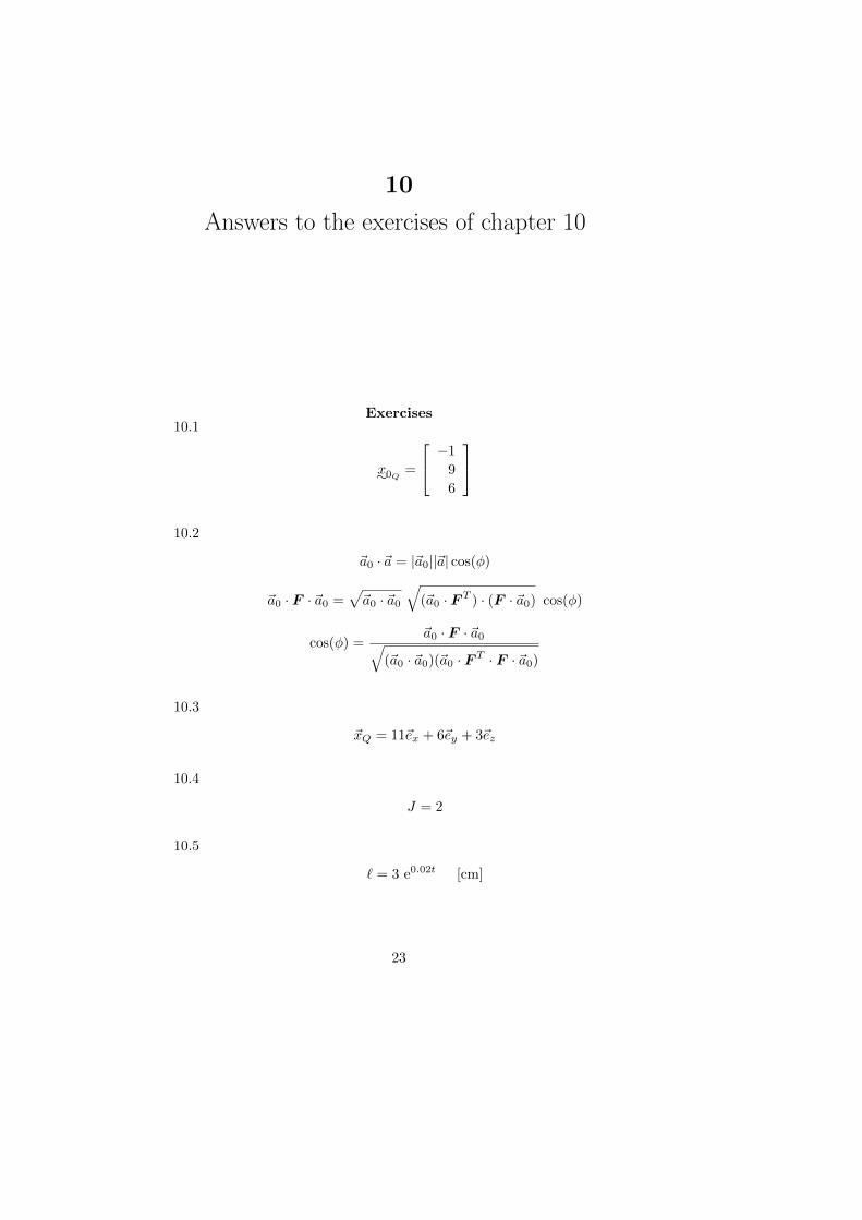
10
Answers to the exercises of chapter 10
Exercises10.1
x∼0Q =
−1
9
6
10.2
~a0 · ~a = |~a0||~a| cos(φ)
~a0 · F · ~a0 =√~a0 · ~a0
√(~a0 · F T ) · (F · ~a0) cos(φ)
cos(φ) =~a0 · F · ~a0√
(~a0 · ~a0)(~a0 · F T · F · ~a0)
10.3
~xQ = 11~ex + 6~ey + 3~ez
10.4
J = 2
10.5
` = 3 e0.02t [cm]
23

24 Answers to the exercises of chapter 10
10.6
εF =1
2
(F · F T + F · F T
)=
1
2
(F · F−1 · F · F T + F · F T · F−T · F T
)=
1
2
(L ·B +B ·LT
)
11
Answers to the exercises of chapter 11
Exercises11.1
ρAVA = ρBVB
11.2
ρ =1500
1 + 0.02texpressed in [kg/m3]
25

12
Answers to the exercises of chapter 12
Exercises12.1
εv = 1/8
12.2
Fv = −65
24G`2
12.3
E =5 h Kv
6π δ R2
12.4
ν = 0.2
12.5 (a) εyy = 0.1
(b) εxx = −0.067
(c) σyy = 0.8 [MPa]12.6
ε =1
2
αR
L(~ex~ez + ~ez~ex)
σ = − E
2(1 + ν)
αR
L(~ex~ez + ~ez~ex)
σM =E
2(1 + ν)
αR
L
√3
26

13
Answers to the exercises of chapter 13
Exercises
13.1 The surfaces with a normal in y-direction are stress free. So at
these surfaces σyz = σzy = 0. This contradicts the assumptions
on the stress field that were given.
13.2 Rigid body motions of the plate are not suppressed.
13.3 The following requirements are not satisfied:
• Local force equilibrium in x-direction.
• The ”oblique” sides of the trapezium shaped plate are not
stress free.
13.4
c2 = − 6P
hb3; c1 =
12P
hb3
13.5 The given velocity field leads to a flow where all fluid parti-
cles rotate around the z-axis with the same angular velocity α.
This means that the position with respect to each other of the
particles does not change and so D = 0. Every fluid particle
moves uniformly along a circular track around the z-axis in a
plane parallel to the xy-plane. This means that every particle
has an acceleration with magnitude α2r with r =√x2 + y2 in
the direction of the z-axis. To realize this acceleration a force
per unit mass ~q in the direction of the z-axis is necessary.
13.6 For the points x = ±a, y = b the fluid velocity is not uniquely
27

28 Answers to the exercises of chapter 13
defined. From a view point based on the rigid wall: ~v = ~0.
When looking at the moving wall ~v = V ~ex.
13.7 The requirement that no fluid can pass the wall of the vessel is
not satisfied.
13.8
~q = −α2 (x~ex + y~ey)

14
Answers to the exercises of chapter 14
Exercises
14.1 (a) Since:
p∼=
1
x...
xn
for n = 1 the matrix K can be elaborated as:
K =
∫ 1
0
p∼p∼T dx =
∫ 1
0
[1 x
x x2
]dx =
[1 1
212
13
]Likewise:
f∼=
∫ 1
0
p∼f dx =
∫ 1
0
[1
x
]3 dx =
[332
]From Ka∼= f∼ it can be derived:
a∼=
[3
0
](c) % Exercise 14.1
clear all ; close all
x=0:0.01:1 ;
xmax=length(x) ;
% Exact function
for i=1:xmax
if x(i)<=0.5
f(i)=1;
29

30 Answers to the exercises of chapter 14
else
f(i)=0;
end
end
plot(x,f,’r-’);
grid on ; xlabel(’x’) ; ylabel(’h(x)’) ;
title(’Answer to exercise 1’)
hold on
% loop for different order of the polynomial from n=2 to n=10
for n=2:10
f=zeros(n+1,1); K=zeros(n+1,n+1);
for i=1:n+1
f(i)=(1/i)*(0.5)^i;
for j=1:n+1
K(i,j)=1/(i+j-1);
end
end
a=inv(K)*f; condnum(n)=cond(K); plot(x,polyval(a(n+1:-1:1),x),’b-’)
end
% graph of condition number against order of the polynomial
figure ; plot(condnum) ; xlabel(’polynomial order’) ;
ylabel(’condition number’)
For a number of values of n the interpolation polynomial h(x)
is given in figure 14.1.
14.2 The weighted residuals form is given by:∫ b
a
w
[u+
du
dx+
d
dx(cdu
dx) + f
]dx = 0
After partial integration we find the so-called weak form∫ b
a
w
[u+
du
dx
]dx−
∫ b
a
dw
dxcdu
dxdx = −
∫ b
a
wf dx− wcdu
dx
∣∣∣∣ba
14.3 % Exercise 14.3
clear all ; close all ; clf
n=10; delt=1/(n-1); x=0:delt:1;
for i=1:n
if x(i)<=0.5

Exercises 31
0 0.1 0.2 0.3 0.4 0.5 0.6 0.7 0.8 0.9 1−0.4
−0.2
0
0.2
0.4
0.6
0.8
1
1.2
1.4
x
h(x
)
Answer to exercise 1
Fig. 14.1. h(x) for a number of different polynomial orders
g(i)=1;
else
g(i)=0;
end
for j=1:n
K(i,j)=x(i)^(j-1);
end
end
a=inv(K)*g’;
% for plotting purposes functions are defined at finer intervals
xx=0:0.01:1
for i=1:length(xx)
if xx(i)<=0.5
gg(i)=1;
else
gg(i)=0;
end
end
plot(xx,polyval(a(n:-1:1),xx),’b-’)
title([’Approximation for polynomial of order ’,num2str(n)])
xlabel(’x’); ylabel(’h(x)’); hold on ; grid on

32 Answers to the exercises of chapter 14
plot(xx,gg,’r-’)
The matrix is given in the lecture notes. The polynomial fit
for a polynomial of order 10 is given in figure 14.2. There is a
substantial difference between this fit and the one given in figure
14.1. The fit of figure 14.2 captures precisely the points f(xi),
which is not the case for the fit based on the weighted residuals
form. Moreover, although the fit of figure 14.2 is exact at these
points, the average deviation from f(x) is much larger than in
figure 14.1.
0 0.1 0.2 0.3 0.4 0.5 0.6 0.7 0.8 0.9 1−1
−0.5
0
0.5
1
1.5
2Approximation for polynomial of order 10
x
h(x
)
Fig. 14.2. polynomial fit of order 10
14.4 (a)
a0 = u2
a1 =1
2(u3 − u1)
a2 =1
2(u1 + u3 − 2u2)
(b) The shape functions are:
N1 = −1
2x(1− x)
N2 = (1 + x)(1− x)

Exercises 33
N3 =1
2x(1 + x)
(d) No, as uh(xi) should be equal to ui.
(e) No, same reason
14.5 (a) ∫ h1+h2
x=0
dw
dxcdu
dxdx = −
∫ h1+h2
x=0
wdx+ wcdu
dx
∣∣∣∣h1+h2
0
for all w(x)
(b)
N11 = 1− x
h1
N12 =
x
h1
N21 = − 1
h2x+ 1 +
h1h2
N22 =
1
h2x− h1
h2
(f)
c
1h1
0 − 1h1
0 1h2
− 1h2
− 1h1− 1h2
1h1
+ 1h2
0
0
u3
= −1
2
h1+?
h2+?
h1 + h2
c
(1
h1+
1
h2
)u3 = −1
2(h1 + h2)
u3 = −h1h22c
14.6 (b)
dNidx
=dNidξ
dξ
dx
(c)
dξ
dx=
132 + ξ

34 Answers to the exercises of chapter 14
(d)
h1 = −1
6
14.7 (a) % Adjusted demo_fem1d for exercise 7%
clear, close all
%------ Define the mesh, material properties and boundary conditions ------
% The domain spans xmin <= x <= xmax
xmin= 0;
xmax= 1;
% number of elements
nelem= 5;
% norder: order of the interpolation polynomial
% norder=1, linear element
% norder=2, quadratic element
norder=1;
% generate the mesh
if norder==1,
% simple 1d uniform mesh, coordinates
dx=(xmax-xmin)/nelem;
coord=(xmin:dx:xmax)’;
% element topology
top=[(1:nelem)’ (2:nelem+1)’ ones(nelem,2)];
elseif norder==2,
% again a simple 1d uniform mesh,
% coordinates:
dx=(xmax-xmin)/(2*nelem);
coord=(xmin:dx:xmax)’;
% element topology
top=[(1:2:nelem*2)’ (2:2:(nelem*2+1))’ (3:2:(nelem*2+2))’ ones(nelem,2)];
end
% materials properties and some other useful information
% if c<0: a non-constant c is generated by elm1d_c,

Exercises 35
% else elm1d_c returns c
c=1;
f=0;
mat.mat(1)=c; % c
mat.mat(3)=f; % f
mat.mat(4)=norder; % element order
mat.types=[’elm1d’];
% boundary conditions: u=0 at left end
bndcon=[1 1 0]; % [node number ; degree of freedom ; value ]
% nodal forces f=1 at right end
nodfrc=[6 1 1]; % [node number ; degree of freedom ; value ]
%------ Solve the problem using the 1D fem program FEM1D ------
fem1d
%------ postprocess the data ------
%* plot the solution (sol) as well as the exact solution (u_exact)
subplot(1,2,1),
plot(coord,sol,’-’);
xlabel(’x’), ylabel(’u’);
nel=num2str(nelem);
sorde=num2str(norder);
tekst=[’aantal elementen = ’,nel,’ orde van elementen = ’,sorde]
title(tekst)
subplot(1,2,2)
if norder==1,
plot([coord(1:nelem) coord(2:nelem+1)]’,sigma’)
elseif norder==2,
plot([coord(1:2:2*nelem) coord(2:2:2*nelem+1)
coord(3:2:2*nelem+2)]’,sigma’)
end
xlabel(’x’), ylabel(’\sigma’);
(b) ii=pos(2,:) ; u = sol(nonzeros(ii)) ; u = [0.2 ; 0.4]
(c) ii=dest(3,:) ; u=sol(ii) ; u=0.4
36 Answers to the exercises of chapter 14
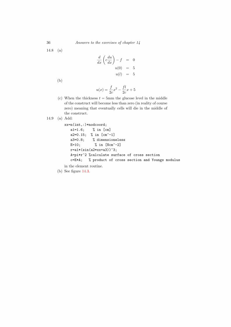
14.8 (a)
d
dx
(cdu
dx
)− f = 0
u(0) = 5
u(l) = 5
(b)
u(x) =f
2cx2 − fl
2cx+ 5
(c) When the thickness t = 5mm the glucose level in the middle
of the construct will become less than zero (in reality of course
zero) meaning that eventually cells will die in the middle of
the construct.
14.9 (a) Add:
xx=n(int,:)*nodcoord;
a1=1.6; % in [cm]
a2=0.15; % in [cm^-1]
a3=0.8; % dimensioneless
E=10; % in [Ncm^-2]
r=a1*(sin(a2*xx+a3))^3;
A=pi*r^2 %calculate surface of cross section
c=E*A; % product of cross section and Youngs modulus
in the element routine.
(b) See figure 14.3.

Exercises 37
0 2 4 6 8 10 120
1
2
3
4
5
6
7
x
u
Fig. 14.3. Exercise 14.9: Displacement as a function of x

15
Answers to the exercises of chapter 15
Exercises
15.1 (b) See Fig. 15.1. For small a the solution is approximately the
same as the solution of the diffusion equation. For larger a
particles drag along with the fluid and thus the higher con-
centrations shift to the right. For values higher than 10 the
solution becomes unstable.
0 0.1 0.2 0.3 0.4 0.5 0.6 0.7 0.8 0.9 10
0.1
0.2
0.3
0.4
0.5
0.6
0.7
0.8
0.9
1
x
u
a = 0.001
(a)
0 0.1 0.2 0.3 0.4 0.5 0.6 0.7 0.8 0.9 10
0.1
0.2
0.3
0.4
0.5
0.6
0.7
0.8
0.9
1
x
u
a = 1
(b)
0 0.1 0.2 0.3 0.4 0.5 0.6 0.7 0.8 0.9 10
0.5
1
x
u
a = 10
(c)
0 0.1 0.2 0.3 0.4 0.5 0.6 0.7 0.8 0.9 1−0.4
−0.2
0
0.2
0.4
0.6
0.8
1
x
u
a = 20
(d)
Fig. 15.1. Solution of the steady convection diffusion equation for differentvalues of a using 5 linear elements
38

Exercises 39
(c) With h = 0.2 and c = 1 it follows that Peh > 1 if a > 10.
15.2 (a) It can be seen that using θ = 0.5 the solutions remain stable,
even for large time steps. When θ < 0.5 the solution starts
to oscillate when the time step becomes to large.
(b) When a > 20 solutions will become unstable.
(c) When ∆t = 0.001 the discretization of u no longer allows an
”exact” description of the u as a function of x.
(d) Reducing the convective velocity does not influence the sta-
bility much. Increasing the number of elements (i.e. reducing
the size of an element) again leads to stable solutions.
0 0.2 0.4 0.6 0.8 1−1
−0.5
0
0.5
1
x
u
Fig. 15.2. Solution for different time steps
15.3 (a) Initial conditions. Use sol(:,1) (second index is the time step)
For initial conditions the following script can be used:
for inode = 1: nnodes
idof=dest(inode,1)
x = coord(inode,1)
sol(idof,1)=sin(2*pi*x)
end
Essential boundary condition u = 0 at x = 0;
bndcon=[1 1 0]

40 Answers to the exercises of chapter 15
Natural boundary condition: c ∂u/∂x = 0 at x = 1. It is not
necessary to prescribe this, because default this condition is
set when no essential boundary conditions are prescribed.
(b) The same as in item (a) but with different initial conditions.
15.4 (a) For the initial condition add the lines:
ii=find(coord>0.0001) % excludes the point at x=0
sol(dest(ii,1))=1000;
This change can be made in the file: fem1dcd or in demo_fem1dcd.
Boundary condition:
bndcon=[1 1 0];
0 0.001 0.002 0.003 0.004 0.005 0.006 0.007 0.008 0.009 0.010
100
200
300
400
500
600
700
800
900
1000
x
u
a = 1e−011
(a)
0 0.5 1 1.5 2 2.5 3 3.5 4
x 104
400
500
600
700
800
900
1000
t
pre
ssu
re
(b)
Fig. 15.3. Solution of the confined compression problem a) pressure as a func-tion of space and time, b) pressure near indenter as a function of time

16
Answers to the exercises of chapter 16
Exercises
16.1 (a) The answers to items (a) to (c) can be determined manually
or by means of MATLAB. The enclosed answer is by the use
of MATLAB. The following .m-file was used:
% Answer to exercise 16.1 a) to c) by means of matlab
%location of integration points in local coordinates
%ichoice = 1 ; Gauss integration ; ichoice = 2 Newton Cotes
clear all
ichoice=1;
switch ichoice
case 1
a=1/sqrt(3);
xicol= [-a ; a ; a ; -a];
etacol=[-a ; -a ; a ; a];
w=[1 1 1 1];
case 2
xicol= [-1 ; 1 ; 1 ; -1];
etacol=[-1 ; -1 ; 1 ; 1];
w=[1 1 1 1];
end
coord=[-2 -2 ;
2 -2 ;
2 2 ;
-2 2 ];
M=zeros(4); C=zeros(4);
41

42 Answers to the exercises of chapter 16
%loop over integration points
for i=1:4
xi=xicol(i) ; eta=etacol(i);
% Equation (16.42)
N=[0.25*(1-xi)*(1-eta) ;
0.25*(1+xi)*(1-eta) ;
0.25*(1+xi)*(1+eta) ;
0.25*(1-xi)*(1+eta) ];
dNdxi = [-0.25*(1-eta) ;
0.25*(1-eta) ;
0.25*(1+eta) ;
-0.25*(1+eta) ];
dNdeta= [-0.25*(1-xi) ;
-0.25*(1+xi) ;
0.25*(1+xi) ;
0.25*(1-xi) ];
% Equation (16.48)
dxdxi = dNdxi’ * coord(:,1);
dxdeta = dNdeta’* coord(:,1);
dydxi = dNdxi’ * coord(:,2);
dydeta = dNdeta’* coord(:,2);
% Equation (16.47)
matxxi=[dxdxi dxdeta ;
dydxi dydeta];
% Equation (16.50)
j=det(matxxi);
% Equation (16.49)
matdxidx=inv(matxxi);
dxidx=matdxidx(1,1);

Exercises 43
detadx=matdxidx(1,2);
%Equations (16.37) and (16.51)
M=M+N*N’*j*w(i);
C=C+N*(dNdxi’*dxidx+dNdeta’*detadx)*j*w(i);
end
(d) In this case it is easiest to work with a global coordinate sys-
tem. In the global system the shape function can be written
in the following form:
N1 =1
16(2− x)(2− y)
N2 =1
16(2 + x)(2− y)
N3 =1
16(2 + x)(2 + y)
N4 =1
16(2− x)(2 + y)
N1 and N4 are 0 on the right-hand side. This leads to:
∫ 2
−2
0
14 (2− y)14 (2 + y)
0
q dx =
0
2
2
0
q
16.2 (a) No, topology is not unique
(b) pos= [ 5 7 12 10 ]
(c) dest= [1 2 3 .... 16]
(d) ii = nonzeros(pos(8,:))
ulem=sol(ii)
(e) ii=dest(nodes,:)
ulem=sol(ii)
(f)
N1 =1
4(1− ξ)(1− η)

44 Answers to the exercises of chapter 16
N2 =1
4(1 + ξ)(1− η)
N3 =1
4(1 + ξ)(1 + η)
N4 =1
4(1− ξ)(1 = η)
u(1
4,
3
4) = 4.3
(g)
u∼Te = [3 7 1 4]
16.3 (a) No heat flow through these boundaries.
(b) % Solution of exercise 3.3
%mesh generation
lx=1; % length of the domain
h=1; % height of the domain
points=[
0 0;
1 0;
1 1;
0 1];
n=5; % number of elements in the x-direction
m=5; % number of elements in the y-direction
curves=[
1 2 n 1 1
2 3 m 1 1
3 4 n 1 1
4 1 m 1 1];
subarea=[1 2 3 4 1];
norder=1; % 1: bi-linear elements, 2: bi-quadratic elements
% create the mesh
[top,coord,usercurves]=crmesh(curves,subarea,points,norder);

Exercises 45
% define the mat file
mat.mat(1)=1;
mat.mat(2)=1; %Adjust elcd_a so ax is given the value of mat.mat(2)
mat.mat(3)=0;
mat.mat(11)=norder+2;
mat.types=’elcd’; % convection diffusion element
% inflow boundary
bndcon=[];
crv=4;
dof=1;
iplot=0;
string=’0’;
bndcon=addbndc(bndcon,coord,top,mat,usercurves,crv,dof,string,iplot);
% outflow boundary
crv=2;
dof=1;
iplot=0;
string=’1’;
bndcon=addbndc(bndcon,coord,top,mat,usercurves,crv,dof,string,iplot);
istat=1; % 1: steady state solution, 2: unsteady solution
femlin_cd
figure(1)
if istat==1,
conoddat(sol(dest),coord,top,mat);
else
for i=1:4
subplot(2,2,i)
conoddat(sol(dest,2*i),coord,top,mat);
title([’t=’ num2str(2*i*dt)]);
end
end
(c) ii=nonzeros(usercurves(1,:))
u=sol(dest(ii))

46 Answers to the exercises of chapter 16
u=[0 0.1286 0.2859 0.4780 0.7129 1.000]
(d) The same result.
16.4 % Exercise 16.4
points=[0 0; 10 0; 10 2; 0 2 ; 0 -1; 10 -1];
n=10; % number of elements in the x-direction
m=3; % number of elements on gam2
mm=5 ; % number of elements on gam5
curves=[5 6 n 1 1
6 2 m 1 1
2 1 n 1 1
1 5 m 1 1
2 3 mm 1 1
3 4 n 1 1
4 1 mm 1 1];
subarea=[1 2 3 4 1 ; -3 5 6 7 1 ];
norder=1; % 1: bi-linear elements, 2: bi-quadratic elements
% create the mesh
[top,coord,usercurves]=crmesh(curves,subarea,points,norder);
% define the mat file
mat.mat(1)=1;
mat.mat(2)=1;
mat.mat(3)=0;
mat.mat(11)=norder+2;
mat.types=’elcd’; % convection diffusion element
% inflow boundary
bndcon=[]; crv=1; dof=1; iplot=0; string=’1’;
bndcon=addbndc(bndcon,coord,top,mat,usercurves,crv,dof,string,iplot);
% outflow boundary
crv=7; dof=1; iplot=0; string=’0’;
bndcon=addbndc(bndcon,coord,top,mat,usercurves,crv,dof,string,iplot);
istat=1; % 1: steady state solution, 2: unsteady solution
femlin_cd
conoddat(sol(dest),coord,top,mat);
For the condition for ~a the file elcd a.m has to be changed:
function [ax,ay]=elcd_a(x,y,fx,fy);
ax=0;
ay=0;

Exercises 47
if y>0
ax=y;
end

17
Answers to the exercises of chapter 17
Exercises
17.1 fdgfghfsh
(c)
ξ η j = det(x,ξ)0 0 5.75
0.5 0.5 5.6251 0 61 -1 6.5
Table 17.1. element 1
ξ η j = det(x,ξ)0 0 2
0.5 0.5 1.6251 0 0.125-1 1 -1
Table 17.2. element 2
For element 2 the point (-1,1) renders a negative Jacobian
determinant, meaning that the element is locally inside-out.
17.2 (a)
N1 =1
4(1− ξ)(1− η)
48
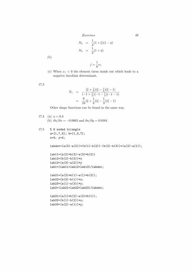
Exercises 49
N2 =1
4(1 + ξ)(1− η)
N3 =1
2(1 + η)
(b)
j =1
8x1
(c) When x1 < 0 the element turns inside out which leads to a
negative Jacobian determinant.
17.3
N1 =(ξ + 1
3 )(ξ − 13 )(ξ − 1)
(−1 + 13 )(−1− 1
3 )(−1− 1)
=9
16(ξ +
1
3)(ξ − 1
3)(ξ − 1)
Other shape functions can be found in the same way.
17.4 (a) u = 0.4
(b) ∂u/∂x = −0.0863 and ∂u/∂y = 0.0164
17.5 % 6 noded triangle
a=[1,7,5]; b=[1,3,7];
x=4; y=4;
labdet=(a(3)-a(2))*(b(1)-b(2))-(b(2)-b(3))*(a(2)-a(1));
lab11=(a(2)*b(3)-a(3)*b(2))
lab12=(b(2)-b(3))*x
lab13=(a(3)-a(2))*y
lab1=(lab11+lab12+lab13)/labdet;
lab21=(a(3)*b(1)-a(1)*b(3));
lab22=(b(3)-b(1))*x;
lab23=(a(1)-a(3))*y;
lab2=(lab21+lab22+lab23)/labdet;
lab31=(a(1)*b(2)-a(2)*b(1));
lab32=(b(1)-b(2))*x;
lab33=(a(2)-a(1))*y;

50 Answers to the exercises of chapter 17
lab3=(lab31+lab32+lab33)/labdet;
icheck=lab1+lab2+lab3 % icheck should be 1
N=[ lab1*(2*lab1-1);
lab2*(2*lab2-1);
lab3*(2*lab3-1);
4*lab1*lab2;
4*lab2*lab3;
4*lab1*lab3]
u=[2 ; 5 ; 3 ; 2 ; 0 ; 2]
u44=N’*u
leads to: u44 = 0.8367

18
Answers to the exercises of chapter 18
Exercises18.1 (a)
tr(ε) = εxx + εyy
(b)
tr(ε) = εxx + εyy + εzz
εzz can be eliminated with the constitutive law
(c) Plane stress: σxx, σyy, σxy, εxx, εyy, εzz, εxy(d) Plane strain: σxx, σyy, σzz, σxy, εxx, εyy, εxy(e)
σxxσyyσxyσzz
=
κ+ 4
3G κ− 23G 0 κ− 2
3G
κ− 23G κ+ 4
3G 0 κ− 23G
0 0 2G 0
κ− 23G κ− 2
3G 0 κ+ 43G
εxxεyyεxyεzz
Let κ − 2
3G = β and κ + 43G = α. With σzz = 0 and the
constitutive law εzz can be written as a function of εxx and
εyy. This will lead to:
H =
α− β2
α β − β2
α 0
β − β2
α α− β2
α 0
0 0 2G
(f) Use
κ =E
3(1− 2ν)
51

52 Answers to the exercises of chapter 18
and
G =E
2(1 + ν)
Stress depends linearly on E.
18.2 (a)
top =
[1 3 4
1 2 3
]
(b)
pos =
[1 2 5 6 7 8
1 2 3 4 5 6
]
(c)
dest =
1 2
3 4
5 6
7 8
(d) The matrix can be formed manually, but also by writing a
short Matlab program: A program could be:
pos = [1 2 5 6 7 8 ; 1 2 3 4 5 6 ]
K=zeros(8);
k1e=zeros(6)+1;
k2e=zeros(6)+2;
%contribution element 1
ii=nonzeros(pos(1,:));
K(ii,ii)=K(ii,ii)+k1e;
%contribution element 2
ii=nonzeros(pos(2,:));
K(ii,ii)=K(ii,ii)+k2e;
K
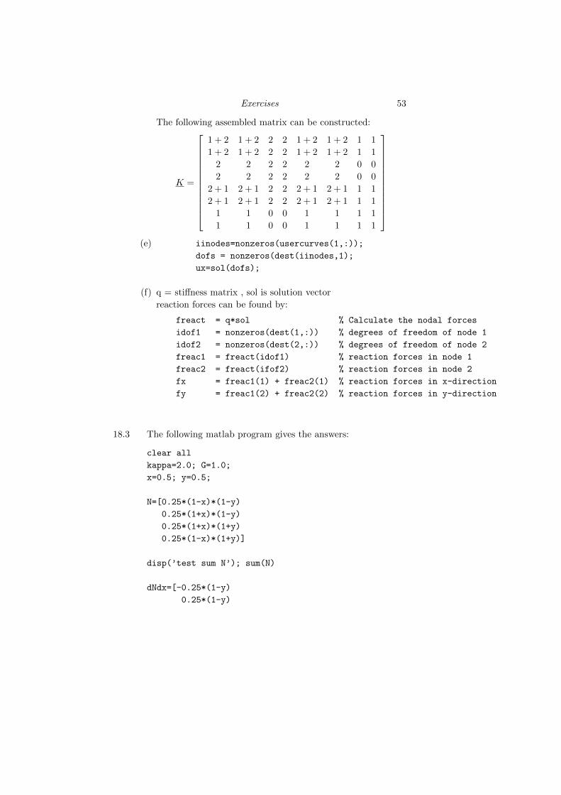
Exercises 53
The following assembled matrix can be constructed:
K =
1 + 2 1 + 2 2 2 1 + 2 1 + 2 1 1
1 + 2 1 + 2 2 2 1 + 2 1 + 2 1 1
2 2 2 2 2 2 0 0
2 2 2 2 2 2 0 0
2 + 1 2 + 1 2 2 2 + 1 2 + 1 1 1
2 + 1 2 + 1 2 2 2 + 1 2 + 1 1 1
1 1 0 0 1 1 1 1
1 1 0 0 1 1 1 1
(e) iinodes=nonzeros(usercurves(1,:));
dofs = nonzeros(dest(iinodes,1);
ux=sol(dofs);
(f) q = stiffness matrix , sol is solution vector
reaction forces can be found by:
freact = q*sol % Calculate the nodal forces
idof1 = nonzeros(dest(1,:)) % degrees of freedom of node 1
idof2 = nonzeros(dest(2,:)) % degrees of freedom of node 2
freac1 = freact(idof1) % reaction forces in node 1
freac2 = freact(ifof2) % reaction forces in node 2
fx = freac1(1) + freac2(1) % reaction forces in x-direction
fy = freac1(2) + freac2(2) % reaction forces in y-direction
18.3 The following matlab program gives the answers:
clear all
kappa=2.0; G=1.0;
x=0.5; y=0.5;
N=[0.25*(1-x)*(1-y)
0.25*(1+x)*(1-y)
0.25*(1+x)*(1+y)
0.25*(1-x)*(1+y)]
disp(’test sum N’); sum(N)
dNdx=[-0.25*(1-y)
0.25*(1-y)

54 Answers to the exercises of chapter 18
0.25*(1+y)
-0.25*(1+y)]
dNdy=[-0.25*(1-x)
-0.25*(1+x)
0.25*(1+x)
0.25*(1-x)]
disp(’test sum dNdxy’);
sum(dNdx)
sum(dNdy)
B=[dNdx(1) 0 dNdx(2) 0 dNdx(3) 0 dNdx(4) 0
0 dNdy(1) 0 dNdy(2) 0 dNdy(3) 0 dNdy(4)
dNdy(1) dNdx(1) dNdy(2) dNdx(2) dNdy(3) dNdx(3) dNdy(4) dNdx(4)]
u=[0 0 0 0 1 0 1 0]’
eps=B*u
H1=kappa*[1 1 0 ; 1 1 0 ; 0 0 0]
H2=(G/3)*[4 -2 0 ; -2 4 0 ; 0 0 3]
H=H1+H2;
sig=H*eps
18.4 (a) for an element with 4 nodes:
inodes=top(ielem,1:4)
idof=dest(inodes,:);
u=sol(idof);
This leads to a matrix u with two columns. The first col-
umn gives the x-displacements, the second column the y-
displacements
(b) and (c) This can be done when the shape functions N(ξ, η) are known
and the coordinates ξ and η of the integration point are
known. First the displacements have to be stored in one col-
umn:
ucol=zeros(8,1)
for i=1:4
ucol(2*i-1)= u(i,1)
Exercises 55
ucol(2*i) = u(i,2)
end
Then the strain can be calculated by means of (also see exer-
cise: 5.3):
eps=B*ucol
sig=H*eps
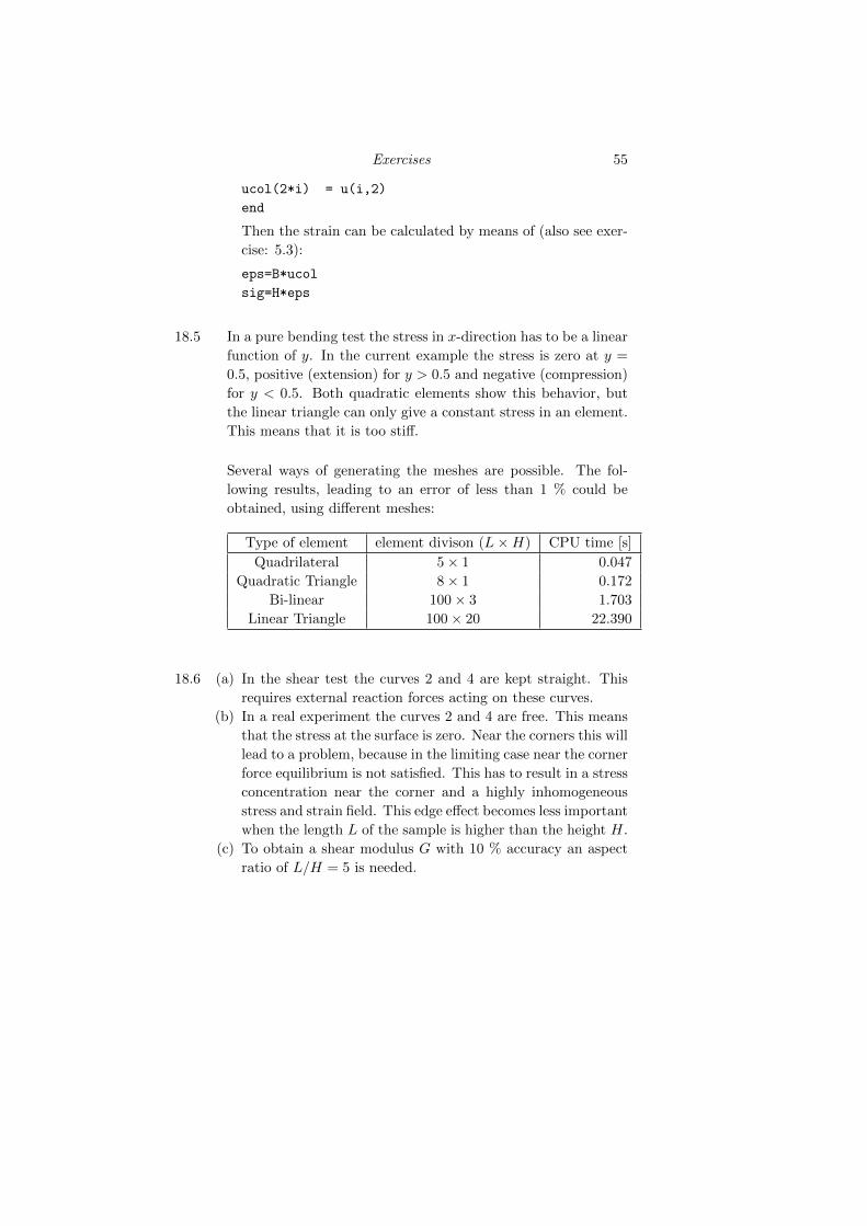
18.5 In a pure bending test the stress in x-direction has to be a linear
function of y. In the current example the stress is zero at y =
0.5, positive (extension) for y > 0.5 and negative (compression)
for y < 0.5. Both quadratic elements show this behavior, but
the linear triangle can only give a constant stress in an element.
This means that it is too stiff.
Several ways of generating the meshes are possible. The fol-
lowing results, leading to an error of less than 1 % could be
obtained, using different meshes:
Type of element element divison (L×H) CPU time [s]
Quadrilateral 5× 1 0.047
Quadratic Triangle 8× 1 0.172
Bi-linear 100× 3 1.703
Linear Triangle 100× 20 22.390
18.6 (a) In the shear test the curves 2 and 4 are kept straight. This
requires external reaction forces acting on these curves.
(b) In a real experiment the curves 2 and 4 are free. This means
that the stress at the surface is zero. Near the corners this will
lead to a problem, because in the limiting case near the corner
force equilibrium is not satisfied. This has to result in a stress
concentration near the corner and a highly inhomogeneous
stress and strain field. This edge effect becomes less important
when the length L of the sample is higher than the height H.
(c) To obtain a shear modulus G with 10 % accuracy an aspect
ratio of L/H = 5 is needed.


![ANSWERS TO ODD-NUMBERED EXERCISES M207 - Ougouagougouag.com/AnsOdds-M207.pdf · 2017-11-27 · Answers to Odd-Numbered Exercises 47. APPENDIX I ANSWERS TO EXERCISES 37. [o, 4] A63](https://img.dokumen.tips/doc/110x75/5ea264aa5c19072f7a5c9a88/answers-to-odd-numbered-exercises-m207-2017-11-27-answers-to-odd-numbered-exercises.jpg)