BIOMASS BURNING AND NATURAL EMISSIONS IN THE …mtc-m21b.sid.inpe.br/col/sid.inpe.br/mtc-m21b/2017/05.29.14.21/doc/pub... · CataloginginPublicationData Santos,FernandoCavalcantedos

sid.inpe.br/mtc-m21b/2017/05.29.14.21-TDI

BIOMASS BURNING AND NATURAL EMISSIONS INTHE BRAZILIAN AMAZON RAINFOREST: IMPACT

ON THE OXIDATIVE CAPACITY OF THEATMOSPHERE

Fernando Cavalcante dos Santos

Doctorate Thesis of the GraduateCourse in Earth System Science,guided by Drs. Karla Maria Longode Freitas, and Alex Guenther,approved in May 31, 2017.

URL of the original document:<http://urlib.net/8JMKD3MGP3W34P/3P26AFB>

INPESão José dos Campos

2017

http://urlib.net/8JMKD3MGP3W34P/3P26AFB

PUBLISHED BY:

Instituto Nacional de Pesquisas Espaciais - INPEGabinete do Diretor (GB)Serviço de Informação e Documentação (SID)Caixa Postal 515 - CEP 12.245-970São José dos Campos - SP - BrasilTel.:(012) 3208-6923/6921E-mail: [email protected]

COMMISSION OF BOARD OF PUBLISHING AND PRESERVATIONOF INPE INTELLECTUAL PRODUCTION (DE/DIR-544):Chairperson:Maria do Carmo de Andrade Nono - Conselho de Pós-Graduação (CPG)Members:Dr. Plínio Carlos Alvalá - Centro de Ciência do Sistema Terrestre (CST)Dr. André de Castro Milone - Coordenação de Ciências Espaciais e Atmosféricas(CEA)Dra. Carina de Barros Melo - Coordenação de Laboratórios Associados (CTE)Dr. Evandro Marconi Rocco - Coordenação de Engenharia e Tecnologia Espacial(ETE)Dr. Hermann Johann Heinrich Kux - Coordenação de Observação da Terra (OBT)Dr. Marley Cavalcante de Lima Moscati - Centro de Previsão de Tempo e EstudosClimáticos (CPT)Silvia Castro Marcelino - Serviço de Informação e Documentação (SID) DIGITALLIBRARY:Dr. Gerald Jean Francis BanonClayton Martins Pereira - Serviço de Informação e Documentação (SID)DOCUMENT REVIEW:Simone Angélica Del Ducca Barbedo - Serviço de Informação e Documentação(SID)Yolanda Ribeiro da Silva Souza - Serviço de Informação e Documentação (SID)ELECTRONIC EDITING:Marcelo de Castro Pazos - Serviço de Informação e Documentação (SID)André Luis Dias Fernandes - Serviço de Informação e Documentação (SID)

sid.inpe.br/mtc-m21b/2017/05.29.14.21-TDI

BIOMASS BURNING AND NATURAL EMISSIONS INTHE BRAZILIAN AMAZON RAINFOREST: IMPACT

ON THE OXIDATIVE CAPACITY OF THEATMOSPHERE

Fernando Cavalcante dos Santos

Doctorate Thesis of the GraduateCourse in Earth System Science,guided by Drs. Karla Maria Longode Freitas, and Alex Guenther,approved in May 31, 2017.

URL of the original document:<http://urlib.net/8JMKD3MGP3W34P/3P26AFB>

INPESão José dos Campos

2017

http://urlib.net/8JMKD3MGP3W34P/3P26AFB

Cataloging in Publication Data

Santos, Fernando Cavalcante dos.Sa59b Biomass burning and natural emissions in the brazilian

amazon rainforest: impact on the oxidative capacity of theatmosphere / Fernando Cavalcante dos Santos. – São José dosCampos : INPE, 2017.

xxii + 116 p. ; (sid.inpe.br/mtc-m21b/2017/05.29.14.21-TDI)

Thesis (Doctorate in Earth System Science) – InstitutoNacional de Pesquisas Espaciais, São José dos Campos, 2017.

Guiding : Drs. Karla Maria Longo de Freitas, and AlexGuenther.

1. Biogenic volatile organic compounds. 2. Observation andmodeling. 3. Oxidative capacity. I.Title.

CDU 504.7:630*43(811.3)

Esta obra foi licenciada sob uma Licença Creative Commons Atribuição-NãoComercial 3.0 NãoAdaptada.

This work is licensed under a Creative Commons Attribution-NonCommercial 3.0 UnportedLicense.

ii

http://creativecommons.org/licenses/by-nc/3.0/

http://creativecommons.org/licenses/by-nc/3.0/deed.pt_BR

http://creativecommons.org/licenses/by-nc/3.0/deed.pt_BR

http://creativecommons.org/licenses/by-nc/3.0/

iv

v

ACKNOWLEDGEMENTS

We thank the Group Modeling of the Atmosphere and Its Interfaces: Demerval Moreira,

Rodrigo Braz, Luiz Flavio, Madeleine Gacita, Megan Bela, Daniela Franca, Ricardo

Siqueira, Isilda Menezes and Dr. Saulo Freitas; Eliane Gomes Alves; the National

Center for Atmospheric Research for the infrastructure given during the period of

internship and researchers Dr. Louisa Emmons, Dr. James Smith, Dr. Christine

Wiedinmyer, Dr. Jeong-Hu Park, Dr. Peter Haley and Dr. Andrew Turnipseed

especially for their assistance in the quantification of the samples; the Pacific Northwest

National Laboratory for their support and infrastructure provided during the internship,

postdoctoral students Dasa Gu, Haofei Yu, the researchers Dr. Rodica Lindenmaier, Dr.

Manishkumar Shrivastava, Dr. John Shilling and Dr. Beat Schmid.

To my friends in São Paulo, São Carlos, São José dos Campos and other cities and

countries that I lived during these years.

An especial thank to my friends from the Earth System Science Center program! Alex,

Aline, Carla, Gilney, Karine, Lucia, Mabelis, Chica, Michelle, Minella, Pri e Sandro.

To Dr. Karla Longo and Dr. Alex Guenther for guidance, patience, friendship and

motivation provided during the whole period of development of this work. Thank you

for providing me with this personal growth opportunity that goes beyond the academic

knowledge gained in these years of research.

To FAPESP for the financial support. To the NCAR and PNNL for all the financial

support.

To my family for the dedication, love and patience they have had for all these years;

especially in some difficult times.

And to all who contributed in some way to the accomplishment of this work

vi

vii

ABSTRACT

Emitted by vegetation, isoprene (2-methyl-1,3-butadiene) is the most abundant non-

methane hydrocarbons, with an annual global emission calculated ranging from 440 to

660Tg carbon, depending on the driving variables like temperature, solar radiation, leaf

area index and plant functional type. It is estimated, for example, that the natural

compounds like isoprene and terpenes present in the troposphere are about 90% and

50%, respectively, removed from the atmosphere by oxidation performed by hydroxyl

radical (OH). Furthermore, the oxidation products of isoprene may contribute to

secondary organic aerosol (SOA) formation, affecting the climate and altering the

properties and lifetimes of clouds. Considering the importance of these emissions and

the hydroxyl radical reaction in the atmosphere, the SAMBBA (South American

Biomass Burning Analysis) experiment, which occurred during the dry season

(September 2012) in the Amazon Rainforest, provided information about the chemical

composition of the atmosphere through airborne observations. Although primarily

focused on biomass burning flights, the SAMBBA project carried out other flights

providing indirect oxidative capacity data in different environments: natural emission

dominated flights and biomass-burning flights with fresh plumes and aged plumes. In

this study, we evaluate the oxidative capacity of the Amazon rainforest in different

environments, both for the unpolluted and biomass-burning disturbed atmosphere using

the ratio [MVK + MACR]/[Isoprene]. Beyond that, we propose an improvement on the

formulation of indirect OH density calculation, using the photochemical aging

[O3]/[CO] as a parameter. Using a synergistic approach, balancing numerical modeling

and direct observations, the numerical model BRAMS was coupled to MEGAN

emission model to get a better result for isoprene and OH in the atmosphere,

representing the observations during SAMBBA field campaign. In relation to OH

estimation, we observed an improvement in the concentration values using the modified

sequential reaction model, for both biomass burning regimes and background

environment. We also detected a long-range transport events of O3 during SAMBBA

experiment, considering the high levels of O3 in aged plumes at high altitudes (5,500 –

6,500 m), and the detection of an O3 inflow in the Amazon basin from Africa. These

findings support the importance of long-range transport events as a source of O3 into the

troposphere in the Amazon basin, which could even alter the atmospheric composition

within the planetary boundary layer and alter the oxidative capacity in the region. The

model results showed a reasonable agreement for isoprene concentration, although more

investigation needed for the OH simulation.

Keywords: Biogenic Volatile Organic Compounds. Observation and Modeling.

Oxidative Capacity.

viii

ix

EMISSÕES NATURAIS E DE QUEIMADAS NA FLORESTA AMAZÔNIA:

IMPACTO NA CAPACIDADE OXIDATIVA DA ATMOSFERA

RESUMO

Emitido pela vegetação, o isopreno (2-metil-1,3-butadieno) é o hidrocarboneto não-

metânico mais abundante, com uma emissão global anual calculada entre 440 e 660Tg

de carbono, dependendo de variáveis como temperatura, radiação solar, índice de área

foliar e tipo funcional da planta. Estima-se, por exemplo, que os compostos naturais

como isopreno e terpenos presentes na troposfera são cerca de 90% e 50%,

respectivamente, removidos da atmosfera por oxidação realizada por radical hidroxila

(OH). Além disso, os produtos de oxidação do isopreno podem contribuir para a

formação de aerossóis orgânicos secundários (AOS), afetando o clima e alterando as

propriedades e o ciclo hidrológico das nuvens. Considerando a importância dessas

emissões e a reação do radical hidroxila na atmosfera, o experimento SAMBBA (do

inglês, South American Biomass Burning Analysis), que ocorreu durante a estação seca

(setembro de 2012) na Floresta Amazônica, forneceu informações sobre a composição

química da atmosfera através de observações aéreas. Embora focado principalmente nos

voos ocorridos durante a queima de biomassa, o projeto SAMBBA realizou outros voos

que forneceram dados indiretos de capacidade oxidativa em diferentes ambientes: voos

dominados por emissão natural e voos com queima de biomassa com plumas frescas e

envelhecidas. Neste estudo, avaliamos a capacidade oxidativa da floresta amazônica em

diferentes ambientes, tanto para a atmosfera não poluída quanto para atmosfera

perturbada pela queima de biomassa usando a razão [MVK + MACR] / [Isoprene].

Além disso, propomos uma melhoria na formulação do cálculo da densidade indireta de

OH, usando o envelhecimento fotoquímico [O3] / [CO] como parâmetro. Usando uma

abordagem sinérgica, balanceando modelagem numérica e observações diretas, o

modelo numérico BRAMS foi acoplado ao modelo de emissão MEGAN para obter um

melhor resultado para isopreno e OH na atmosfera, representando as observações

durante a campanha do SAMBBA. Em relação à estimativa de OH, observamos uma

melhora nos valores de concentração usando o modelo de reação sequencial modificada,

tanto para os regimes de queima de biomassa quanto para região pristina. Também

detectamos eventos de transporte de longo alcance de O3 durante o experimento

SAMBBA, considerando os altos níveis de O3 em plumas envelhecidas em altitudes

elevadas (5.500 - 6.500 m) e a detecção de um influxo de O3 na bacia amazônica

proveniente da África. Essas descobertas sustentam a importância dos eventos de

transporte de longo alcance como fonte de O3 na troposfera da bacia amazônica, o que

poderia até alterar a composição atmosférica dentro da camada limite planetária e alterar

a capacidade oxidativa da região. Os resultados do modelo mostraram uma correlação

razoável para a concentração de isopreno, embora fosse necessária mais investigação

para a simulação de OH.

Palavras-chaves: Compostos Orgânicos Voláteis Biogênicos. Observação e Modelagem.

Capacidade Oxidativa.

x

xi

LIST OF FIGURES

Pag.

Figure 1.1 Map of the rainforests in the world (dark green). ........................................... 1

Figure 1.2 OH recycling scheme. Photodissociation of ozone leads to primary OH

formation and a subsequent OH reactions with carbon monoxide and VOCs produce

peroxy radicals. In high-NO conditions, OH is recycled (pathway I). In low-NO

conditions, the deposition of peroxides (pathway II) causes a net loss of OH. Pathway

III was suggested by LELIEVELD et al. (2008) and detailed in equations 1.17-1.19.

Pathway IV with unsaturated VOCs also occurs, with little influence on atmospheric

OH. ................................................................................................................................... 7

Figure 3.1 Study area and SAMBBA flights tracks. The red dots indicate the airports

locations. ......................................................................................................................... 16

Figure 3.2 Idealized flight patterns during SAMBBA field campaign........................... 18

Figure 3.3 Aspects of the Research Aircraft................................................................... 20

Figure 3.4 AVAPS/LIDAR rack and the dropsonde launch tube................................... 21

Figure 3.5 Vaisala Dropsonde RD94 equipped with a special parachute. ..................... 22

Figure 3.6 The Radiometer Rack is located in the center of the picture. ....................... 23

Figure 3.7 The Nephelometer/PSAP/Filters Rack. ......................................................... 24

Figure 3.8 Core chemistry rack. ..................................................................................... 25

Figure 3.9 The CPC/CCN/FWVS Rack (left) and the condensation particle counter

(right). ............................................................................................................................. 26

Figure 3.10 Droplet Measurement Technologies dual column cloud condensation nuclei

counter. ........................................................................................................................... 27

Figure 3.11 Low turbulence inlet and whole air sampling rack. .................................... 27

Figure 3.12 Low turbulence inlet (left) and Interior components in the cabin (right) ... 28

Figure 3.13 WAS cylinders, mounted in cases, in the rear cargo hold. ......................... 28

Figure 3.14 Short Wave Spectrometer and Spectral Hemispheric Irradiance

Measurements rack. ........................................................................................................ 29

Figure 3.15 Spectral Hemispheric Irradiance used during SAMBBA campaign. .......... 30

Figure 3.16 Nitrate rack used during SAMBBA campaign............................................ 31

Figure 3.17 The gas chromatograph - mass spectrometer rack. ..................................... 32

Figure 3.18 On the left, average total column cloud fraction cover and temperature (oC)

during SAMBBA campaign in 2012. On the right, the respective anomalies relative to

September, 2004-2014 period. Data from ERA-Interim global atmospheric reanalysis.36

Figure 3.19 Average surface wind field during SAMBBA campaign in 2012. Data from

ERA-Interim global atmospheric reanalysis. ................................................................. 36

xii

Figure 3.20 (a) Number of fires detected from MODIS onboard AQUA and (b) average

CO mixing ratio (ppmv) at 500 hPA from AIR sensor over Amazon during SAMBBA

campaign in 2012. .......................................................................................................... 37

Figure 3.21 Time averaged CO (ppmv) over SAMBBA period (14th of September - 3rd

of October 2012) from AIRS onboard AQUA satellite during daytime: (a) global map at

500 hPa, and (b) cross section of longitude-pressure within the region indicated on the

map on top. ..................................................................................................................... 39

Figure 3.22 Map showing the political boundaries of the Brazilian Amazon and a

satellite image with the location of the sampling station tower K-34 (S-1) relative to

Manaus location. ............................................................................................................. 42

Figure 3.23 Representation of the study site with the K34 tower location. ................... 43

Figure 3.24 Photos of the tower k-34 (on the left), arrival of the sampling equipment by

land (on the right top) and the aircraft Bae-146 overflying K-34 tower during flight

B735 (on the right bottom). ............................................................................................ 44

Figure 3.25 Instrumentation used in the tower k-34: a) adsorbent cartridge, b) main box

of the sampling system flow and c) anemometer. .......................................................... 45

Figure 3.26 Selected chromatogram (SIM mode) from a sample in the tower K-34

showing isoprene (a), alpha-pinene and other trace compounds (a and b), and a possible

detection of sequiterpenes (SQT) in (c). ......................................................................... 47

Figure 3.27 Sub-grid processes resolved in BRAMS. .................................................... 49

Figure 3.28 A chart of the BRAMS system with the chemistry model component. The

gray blocks and the black arrows indicate the codes that make up the BRAMS system

and their outputs, respectively. The white blocks indicate either the input files for the

pre-processing (first line) as the pre-processing outputs (third line), which are also input

files for pre-processing emissions and boundary conditions and routines for composing

the BRAMS model. ........................................................................................................ 53

Figure 3.29 Schematic of MEGAN2.1 model components and driving variables. ........ 55

Figure 3.30 Coupling scheme BRAMS/MEGAN. The current standard use of the

MEGAN model outputs via emission module PREP-CHEM-SRC was preserved as an

option for future simulations (gray box)......................................................................... 57

Figure 3.31 MEGAN framework with subroutine, functions and variables representing

the levels and calls inside the FORTRAN code built from the last MEGAN version. .. 58

Figure 3.32 Grid domains for SAMBBA simulations. Dash line represents the simulated

domain. ........................................................................................................................... 59

Figure 4.1. Isoprene flux and mixing ratio for three days sampling in K-34 tower.

Original data in red and trend line in blue. Photosynthetically active radiation and

temperature conditions were obtained from BRAMS model. ........................................ 64

Figure 4.2 Cross section of CO (on top), NOx (middle) and O3 (on bottom) mixing ratios

(ppbv) for the three different groups: background environment (on the left), fresh smoke

plume (t < 2 hours, on the middle) and aged smoke plume (t > 2 hours, on the right).

xiii

The aircraft data was interpolated from the various vertical profile measurements using

kriging correlation method. Grey lines show the flight tracks. Hour is presented in local

time. ................................................................................................................................ 66

Figure 4.3 On the left, the track of flight B742 that landed in Palmas – TO. The color

bar is representing the measured O3 mixing ratios (ppbv) along the flight track. On the

right, from top to bottom, the altitude, and the O3, NOx, and CO mixing ratios (ppbv)

measured along the same flight track. The red and blue dots are representing the parts of

the flight track classified as fresh (FP) and aged (AP) smoke plumes, respectively. ..... 70

Figure 4.4 (a) Vertical profiles of O3 with the altitude and as a function of ERO3/CO

(color scale) for all SAMBBA flights. (b) Flights identified as a long-range transport of

ozone. .............................................................................................................................. 72

Figure 4.5 Time averaged Ozone (ppmv) from September 24 to 29 2012 retrieved from

AIRS onboard AQUA satellite during daytime at 500 hPa, with 1º x 1º spatial

resolution. ....................................................................................................................... 72

Figure 4.6 Cross section of the isoprene mixing ratio (ppbv) (top) and the

[MVK+MACR+ISOPOOH]/[Isoprene] ratio (bottom) for the three different groups:

background environment (on the left), fresh smoke plume (t < 2 hours, in the middle),

and aged smoke plume (t > 2 hours, on the right). The aircraft data was interpolated

from the various vertical profile measurements using kriging correlation method. White

dashed lines show the flight tracks. Hour is presented in local time. ............................. 74

Figure 4.7 Isoprene, acetonitrile and carbon monoxide mixing ratios (ppbv) as function

of the daytime (local time) for the different chemical regimes previously classified as

background (green dots), smoke fresh plume (red dots), and aged smoke plume (blue

dots). Black dash lines, and the numbers next to them, are representing the mean values

of the measurements taken below 2,000 m of altitude. Hour is presented in local time

(11:00 – 18:00 h). ........................................................................................................... 77

Figure 4.8 Methanol (green dots), acetonitrile (orange dots), and acetaldehyde (blue

dots) mixing ratios (ppbv), and the [MVK+MACR+ISOPOOH]/[Isoprene] ratio (gray

bars), during a plume interception along the flight track B732 in different altitudes. ... 78

Figure 4.9 Density distributions of the ratio [MVK+MACR+ISOPOOH]/[isoprene], at

the altitude layers (a) 1,500 - 2,000 m, (b) 1,000 - 1,500 m, (c) 500 - 1,000 m and (d) 0 -

500 m. The Kernel analysis was carried out considering the classification for

background (BG), aged smoke (AP), and fresh smoke plumes (FP). The number of

samples and mean values for each group are depicted near the color bars. ................... 80

Figure 4.10 Vertical profile of OH concentration (molecules cm-3

) for the different

chemical regimes: background environment (BG), fresh smoke plume (FP), and aged

smoke plume (AP). On top, the sequential reaction model according to the original

approach of Karl et al. (2007), and on bottom, the new approach used in this work.

Blues lines are the trend lines and grey interval represents the level of confidence (0.95)

used. ................................................................................................................................ 82

xiv

Figure 4.11 Average isoprene emissions rate from the model simulations during the

SAMBBA period from 14 September to 03 October 2012: (a) Off-line BRAMS-

MEGAN and (b) Online BRAMS-MEGAN. ................................................................. 84

Figure 4.12 Time series of the isoprene mixing ration (ppbv) from the numerical

simulations during SAMBBA field campaign in the tower K-34 site at the first model

vertical layer. Black line represents BRAMS-MEGAN off-line and green lines

BRAMS-MEGAN coupled online.................................................................................. 85

Figure 4.13 Mean diurnal cycle of isoprene mixing ratio from the model simulations at

the K-34 tower during the SAMBBA period from 14 September to 03 October 2012. . 85

Figure 4.14 Selected sectors based on number of fires detected from MODIS onboard

AQUA during SAMBBA campaign in 2012. ................................................................. 88

Figure 4.15 Time series of the isoprene mixing ratio from the numerical simulations

during SAMBBA field campaign in clean and polluted area (see Figure 4.14) at the first

model vertical layer. ....................................................................................................... 88

Figure 4.16 Vertical profile of the isoprene mixing ration from the numerical

simulations during SAMBBA field campaign in clean and polluted area (see Figure

4.14). ............................................................................................................................... 89

Figure 4.17 Time series of the OH mixing ratio from the numerical simulations during

SAMBBA field campaign in clean and polluted area (see Figure 4.14) at the first model

vertical layer. .................................................................................................................. 90

Figure 4.18 Vertical profile of the OH mixing ratio from the numerical simulations

during SAMBBA field campaign in clean and polluted area (see Figure 4.14). ............ 91

xv

LIST OF TABLES

Pag.

Table 3.1. SAMBBA research flights analyzed in this work. Reference locations are

detailed in the appendix . ................................................................................................ 19

Table 3.2. Instrumental information about selected variables used during the SAMBBA

analysis. .......................................................................................................................... 33

Table 3.3. Key Instruments employed in the SAMBBA field campaign. ...................... 34

Table 3.4. Observations of the ratio O3/CO and plume age in tropical and subtropical

sites. ................................................................................................................................ 40

Table 3.5. K-34 sampling during SAMBBA field campaign. ........................................ 48

Table 3.6. System configuration for SAMBBA simulations. ......................................... 60

Table 4.1. Typical values of airborne measurements: CO, NOx, and O3 mixing ratios in

Amazonia and cerrado areas in Brazil. ........................................................................... 67

Table 4.2. Airborne measurements of isoprene, oxidation ratio

[MVK+MACR+ISOPOOH]/[isoprene], and OH in remote areas and biomass burning

environments worldwide. ............................................................................................... 75

Table 4.3. Pearson correlation coefficient before and after BRAMS-MEGAN coupling.

........................................................................................................................................ 86

xvi

xvii

LIST OF ACRONYMS AND ABBREVIATIONS

ABLE Amazon Boundary Layer Experiment

ACCENT Atmospheric Composition Change the European Network of

Excellence

AIRS Atmospheric Infrared Sounder

AP Aged plume

ATTO Amazonian Tall Tower Observatory

AUTH-Nkua Aristotle University of Thessalonik – National and Kapodistrian

University of Athens

AVAPS Airborne Vertical Atmospheric Profiling System

BARCA Regional Carbon Balance in Amazonia

BG Backgorund

BIOEMI Biogenic Emission Model

BRAMS Brazilian developments on the Regional Atmospheric Modelling

System

BVOC Biogenic Volatile Organic Compounds

CARMA Community Aerosol and Radiation Model for Atmospheres

CCN Cloud Condensation Nuclei

CESM Community Earth System Model

CL Cloud Layer

CLM Community Land Model

CPC Condensation Particle Counter

CPTEC Centro de Previsão de Tempo e Estudos Climáticos

CTM Chemistry Transport Models

ECD Electron Capture Detection

EDGAR Emission Database for Global Atmospheric Research

ER Enhancement Ratio

FGGA Fast Greenhouse Gas Analyzer

FORTRAN FORmula TRANslation

FP Fresh Plume

GABRIEL Guyanas Atmosphere-Biosphere exchange and Radicals Intensive

Experiment with a Learjet

GC-FID Gas Chromatography with Flame Ionization detector

xviii

GC-MS Gas Chromatography with Mass Spectrometry detector

GEIA Global Emissions Inventories Activity

GFED Global Fire Emissions Database

IIR Imaging Infrared Radiometer

IN Ice Nuclei

INPE Instituto Nacional de Pesquisas Espaciais

ISOPOOH Hydroxyhydroperoxides

JULES JointUKLand Environment Simulator

LAI Leaf Area Index

LIDAR Light Detection And Ranging

MACR Methacrolein

MEGAN Model of Emissions of Gases and Aerosols from Nature

MMS Monolithic Miniature Spectrometer

MODIS Moderate-Resolution Imaging Spectroradiometer

MVK Methyl Vinyl Ketone

NCAR National Center for Atmospheric Research

NIST National Institute of Standards and Technology

PAN Peroxyacetyl Nitrate

PAR Photosynthetically Active Radiation

PBL Planetary Boundary Layer

PFT Plant Functional Type

PNNL Pacific Northwest National Laboratory

PSAP Particle Soot Absorption Photometer

PTRMS Proton Transfer Reaction – Mass Spectrometry

RACM Regional Atmospheric Chemistry Mechanism

RAMS Regional Atmospheric Modeling System

REA Relaxed Eddy Accumulation

RELACS Regional Lumped Atmospheric Chemical Scheme

RETRO REanalysis of the TROpospheric

RTIE Real Time Imaging Electronics

SAMBBA South American Biomass Burning Analysis

SCAR-B Smoke/Sulfates, Clouds and Radiation - Brazil

xix

SHIMS Spectral Hemispheric Irradiance

SID Serviço de Informação e Documentação

SOA Secondary Organic Aerosol

SPG Serviço de Pós-Graduação

SWS Short Wave Spectrometer

TDI Teses e Dissertações Internas

TEB Town Energy Budget

TROFFEE Tropical Forest and Fire Emissions Experiment

UKMO UK Met Office

UV Ultraviolet

VBA Visual Basic for Applications

VOC Volatile Organic Compounds

WAS Whole Air Sampling

WRF Weather Research and Forecasting Model

xx

xxi

SUMMARY

Pag.

1 INTRODUCTION AND THEORETICAL REFERENCE ........................... 1

1.1. Tropical forests and volatile organic compounds ....................................... 1

1.2. The oxidative capacity of the atmosphere .................................................. 4

1.3. Numerical modeling of atmospheric chemistry .......................................... 9

1.4. Numerical models of natural emissions .................................................... 11

2 OBJECTIVES .......................................................................................... 13

3 METHODS............................................................................................... 15

3.1. SAMBBA field campaign ............................................................................ 15

3.1.1. Aircraft instrumentation ........................................................................... 19

3.1.1.1. AVAPS Rack ................................................................................................ 21

3.1.1.2. Radiometer Rack ....................................................................................... 22

3.1.1.3. Nephelometer/PSAP/Filters Rack ............................................................. 23

3.1.1.4. Core Chemistry Rack ................................................................................. 25

3.1.1.5. CPC/CCN Rack ............................................................................................ 26

3.1.1.6. WAS Rack ................................................................................................... 27

3.1.1.7. SWS/SHIMS Rack ....................................................................................... 29

3.1.1.8. PTRMS Rack ............................................................................................... 30

3.1.1.9. Nitrate Rack ............................................................................................... 31

3.1.1.10. GC-MS Rack ............................................................................................... 31

3.1.2. Meteorological settings during SAMBBA .................................................. 35

3.1.3. Classification method of flight tracks ........................................................ 38

3.1.4. Method for the OH calculation ................................................................. 41

xxii

3.2. In situ observation: tower K-34 ................................................................. 42

3.3. Modeling system ....................................................................................... 48

3.3.1. BRAMS ....................................................................................................... 48

3.3.2. MEGAN ...................................................................................................... 54

3.3.3. Model development: BRAMS and MEGAN coupling ................................ 56

3.3.4. Model configuration .................................................................................. 59

4 RESULTS ................................................................................................ 63

4.1. Tower K-34 measurements ....................................................................... 63

4.2. SAMBBA airborne measurements ............................................................. 65

4.2.1. Ambient distributions of CO, NOx and O3 ................................................. 65

4.2.2. Long-range transport of O3 ....................................................................... 71

4.2.3. Isoprene and its oxidation ratio ................................................................ 73

4.2.4. OH estimated using the sequential reaction approach ............................ 81

4.3. Model coupling: BRAMS+MEGAN ............................................................. 83

5 CONCLUSIONS ....................................................................................... 93

REFERENCES ................................................................................................. 97

APPENDIX – SUPLEMENTAR INFORMATION .......................................... 113

1

1 INTRODUCTION AND THEORETICAL REFERENCE

1.1. Tropical forests and volatile organic compounds

The Amazon Rainforest is the largest tropical forest in the world encompassing eight

countries (Bolivia, Peru, Ecuador, Colombia, Venezuela, Guyana, Suriname and French

Guiana) in addition to Brazil. The Brazilian Amazon has approximately 4 million km²,

almost half of the national territory (8.5 million km2), displaying a great diversity in its

fauna and flora. Because it is a complex ecosystem, with a large territorial area, high

biodiversity and still has regions where the main environmental characteristics are

preserved, the Amazon Rainforest is the target of different studies in different areas of

knowledge, constituting a singular region of the planet. Like the Amazon Rainforest,

tropical forests all over the planet (Figure 1.1) have striking common characteristics, the

main one being the wide variety of flora and fauna in the world.

Figure 1.1 Map of the rainforests in the world (dark green).

Source: Simmon (2007)

2

Tropical forests have the fundamental function of helping to maintain the planet's

climatic stability, since they play an important role in biological, physical and chemical

processes; and specifically, on the hydrological cycle and the chemical composition of

the atmosphere. These complex and non-linear forest-atmosphere interactions can soften

or amplify global climatic changes of anthropic origin (BONAN, 2008).

Observational and/or modeling studies conducted in different forest regions

(HOFFMANN et al., 1997; THUNIS; CUVELIER, 2000; TOLL; BALDASANO, 2000;

POTTER et al., 2001; XU; WESELY; PIERCE, 2002; KARLIK; CHUNG; WINER,

2003; BELL; ELLIS, 2004; SOLMON et al., 2004; YIN et al., 2004; BYUN et al.,

2005; CARVALHO et al., 2005; CURCI et al., 2009; GUIMARÃES et al., 2009;

FELDMAN et al., 2010; IM et al., 2011; SARTELET et al., 2012; YÁÑEZ-SERRANO

et al., 2015; MISZTAL et al., 2016), with special attention to biogenic volatile organic

compounds (BVOC), are useful for regional and global understanding of the chemistry

of the atmosphere, carbon cycle and climate. The inclusion of BVOC emissions in

numerical chemical transport models and a better understanding of the processes that

control the emissions of these VOCs can result, for example, in an improvement in the

description of the tropospheric ozone and secondary organic aerosol (SOA) formation

processes (PIERCE et al., 1998; POTTER et al., 2001; BELL; ELLIS, 2004; IM et al.,

2011; SARTELET et al., 2012; HERMANSSON et al., 2014).

Techniques of mass flow measurements above the canopy enable direct measurements

of VOC fluxes using turbulent vortex covariance (BOWLING et al., 1998; NÖLSCHER

et al., 2009; TURNIPSEED et al., 2009). Such systems allow for more accurate

estimates of flow and continuous measurements, as well as the possibility of obtaining

information for a wide variety of BVOCs. These measures assist in the assessment and

validation of emission modeling procedures, and may also establish average emission

factors in a given region with a high diversity of species (e.g. tropical forests) (REEVES

et al., 2004).

3

The determination of BVOC in the atmospheric boundary layer assists in the

determination of the degree of reactivity of many chemical compounds. Often, the

concentration levels of VOCs observed in the environment are very low, but with

significant emission flows. Such information is relevant because it indicates that the

chemical compound studied has a considerable importance in the reactions that occur

along its trajectory in the atmosphere, more precisely in the troposphere. Therefore,

environmental concentration measurements are best used when combined with chemical

emission and transport estimates in numerical models.

The Earth’s land, oceans, and ecosystems daily release tons of trace gases and aerosol

particles to the atmosphere, via both natural and anthropogenic processes. Terrestrial

vegetation emits to the atmosphere a significant amount of biogenic volatile organic

compounds (BVOCs), corresponding to 1,150 Tg Carbon per year. The most abundant

BVOC is isoprene (C5H8), with an annual global emission ranging from 440 to 660 Tg

Carbon per year, depending on driving variables such as temperature, solar radiation,

leaf area index, and plant functional type (GUENTHER et al., 2012). In contrast, the

global emission rate of anthropogenic volatile organic compounds (AVOCs) is around

145 Tg Carbon per year (JANSSENS-MAENHOUT et al., 2015). The BVOCs mixing

ratios in the Amazon are variable, with the values ranging from 2.4 to 7.8 ppbv,

depending on location, altitude, and seasonal behavior of radiation, temperature, and

phenology (Yáñez-Serrano et al., 2015 and references therein). Harley et al. (2004), for

example, estimated that about 38% of the plants in the Amazon forest emit isoprene.

Also, studies have shown that the capacity of different plants for producing and storing

isoprenoids is very specific (SHARKEY; WIBERLEY; DONOHUE, 2008;

LAOTHAWORNKITKUL et al., 2009).

Most of the trace compounds that enter in the atmosphere through emissions from the

surface are subjected to an oxidation process, producing chemical species such as sulfur

dioxide (SO2), sulfate (SO42-

), nitrogen oxide (NO), nitric acid (HNO3), carbon

4

monoxide (CO) and carbon dioxide (CO2). This effect of degradation that the

atmosphere exerts on many chemical compounds, led to the stability in the

concentration of the gases present in the current atmosphere, although the human

activity is modifying its composition to a greater or lesser degree, depending on the

species or chemical class of the emitted compound, as well as the intensity of its

emission.

1.2. The oxidative capacity of the atmosphere

The overall concentration of the hydroxyl (OH) radical in the atmosphere is commonly

used to express oxidative capacity and effectively represent the diurnal ability of the

atmosphere to oxidize trace compounds. Due to this characteristic, the importance of the

tropics in global oxidative capacity can be explained especially by the high levels of

radiation and humidity in the atmosphere of these regions (MONKS, 2005; STOHL et

al., 2009). In addition, the oxidative capacity of the atmosphere cannot be studied solely

because of the chemical composition, since the formation of convective systems can

transport species of short life to higher levels in the troposphere, influencing the

availability of these compounds and consequently the occurrence of oxidative reactions

at higher levels (PRINN, 2003). Due to this feature, we can note the importance of the

combination of meteorological and chemical data in the analysis of numerical models.

The troposphere is responsible to chemically transform and remove trace gases due to a

complex chemistry driven by solar UV radiation. This chemistry is also driven by

emissions of gases, such as NO, CO and VOC, leading to the production of O3 and OH.

The hydroxyl radical is the most important oxidizer and a key measure of the capacity

of the atmosphere to oxidize trace gases, influencing the climate, air pollution, and acid

rain. The primary OH source involves water vapor that reacts with a singlet oxygen

5

atom O(1D) that comes from photodissociation of O3 by solar UV radiation at

wavelengths less than 310 nm (PRINN, 2014). In the presence of nitrogen oxides (NO

and NO2), which is a human-related source, significant amount of net production of O3

is found in the troposphere, in agreement to the O3 – NOx – VOC chemistry. To

summarize, the principal catalyzed reactions involving OH and O3 in the troposphere

are shown in equations 1.1 – 1.15.

O3 + UV O2 + O(1D) (1.1)

O(1D) + H2O 2OH (1.2)

Net effect: O3 + H2O O2 + 2OH (1.3)

OH + CO H + CO2 (1.4)

H + O2 HO2 (1.5)

HO2 + NO OH + NO2 (1.6)

NO2 + UV NO + O (1.7)

O + O2 O3 (1.8)

Net effect: CO + 2O2 CO2 + O3 (1.9)

OH + RH R + H2O (1.10)

R + O2 R2 (1.11)

6

RO2 + NO RO + NO2 (1.12)

NO2 + UV NO + O (1.13)

O + O2 O3 (1.14)

Net effect: OH + RH + 2O2 RO + H2O + O3 (1.15)

The atmosphere of the Amazon, in its undisturbed state, oxidizes the BVOCs naturally

emitted by the forest vegetation, recycling some OH and depositing reactive carbon

back to the surface as several oxidation products, including as secondary organic

aerosols (SOA) that has the potential to affect the climate and alter the properties and

lifetimes of clouds. In this way, the cleaning process also acts as a local recycling

mechanism, preventing the loss of essential nutrients from the forest (LELIEVELD et

al., 2008). It is estimated that about 90% of the isoprene and 50% of the terpenes

((C5H8)n) are removed from the atmosphere via oxidation by OH, followed by the

deposition of oxidized VOC and SOA within a timescale of a few hours (MONKS,

2005). In fact, the isoprene is a key compound in many atmospheric chemistry studies,

especially over forest regions, because of its abundance and high reactivity with OH

(BARKET et al., 2004; PRINN, 2014).

For a long time, the traditional understanding was that the unpolluted atmosphere,

defined by low levels of nitrogen oxides (NOx), has low concentrations of OH during

the midday, typically 1–5 x 105 molecules cm

-3. However, known discrepancies

between atmospheric chemistry model results and observations raised the supposition of

a missing sink for OH (WARNEKE et al., 2001; WHALLEY et al., 2013). Recently,

airborne measurements carried out in an unpolluted atmosphere over the Amazon

rainforest found unexpected high oxidative capacity levels, which, complemented

laboratory and numerical modeling studies, led to a different hypothesis for OH

7

production (LELIEVELD et al., 2008). Concentrations of OH around 5.6 (1.9) x 106

molecules cm-3

were measured in the planetary boundary layer (PBL) over the Amazon,

concomitant with CO, NO, and O3 mixing ratios of 113 (13.9) ppbv, 0.02 (0.02)

ppbv, and 18.5 (4.6) ppbv, respectively, values typical of the unpolluted atmosphere.

This work pointed to the reaction of isoprene with peroxy radicals (HO2) as an

alternative pathway to produce OH in an unpolluted environment (LELIEVELD et al.,

2008). The Figure 1.2 represents the major OH formation in the atmosphere and their

subsequent reactions with VOCs.

Figure 1.2 OH recycling scheme. Photodissociation of ozone leads to primary OH formation

and a subsequent OH reactions with carbon monoxide and VOCs produce peroxy radicals. In

high-NO conditions, OH is recycled (pathway I). In low-NO conditions, the deposition of

peroxides (pathway II) causes a net loss of OH. Pathway III was suggested by LELIEVELD et

al. (2008) and detailed in equations 1.17-1.19. Pathway IV with unsaturated VOCs also occurs,

with little influence on atmospheric OH.

Source: Lelieveld et al. (2008).

8

The efficient OH recycling suggested by LELIEVELD et al., (2008) may explain how

the atmospheric oxidation capacity could be sustained in geological warm periods with

abundant vegetation. The equations x-y represents the OH recycling path, as well as the

deposition of organic hydroperoxides under low-NOx condition.

HO2 + RO2 ROOH + O2 [Deposition] (1.16)

Isoprene + OH R (1.17)

R + O2 RO2 (1.18)

RO2(from isoprene) + HO2 OH + other products (1.19)

More recently, significant advances have been made with organic peroxy radicals

produced as intermediates of atmospheric photochemistry, showing the importance of

both HO2 and NO pathways, even in considered low-NO regions to isoprene chemistry.

An accurate understanding of the two pathways is needed for quantitative predictions of

the concentrations of particulate matter, oxidation capacity, and consequent

environmental and climate impacts in pristine forest regions (LIU et al., 2016).

In contrast, there are regions of Amazonia that have been strongly impacted by human

activity. The ongoing deforestation, followed by vegetation burning to open areas for

pasture and agriculture production is the most devastating example. During the austral

winter (from July to October), the Amazonia climate is typically dry and is disturbed

each year by extensive vegetation fires in areas of deforestation and agricultural/pasture

land management, particularly along the so-called deforestation arc, an area of about

500,000 km2 extending from the southwestern to the eastern border of the forest

(ARTAXO et al., 2013). During the fire events, an intricate myriad of chemical and

9

physical processes occurs. The continuous increase in temperature of the fresh biomass

caused by nearby fires can distill species absorbed by plants with low boiling point

(e.g., Tisoprene 307 K), macromolecular bonds can be broken (i.e., low-temperature

pyrolysis), gasification reactions converting carbon in the solid char to CO and CO2 can

occur and the flames efficiently oxidize the volatile gases to species such as H2O, CO2,

and NOx (BERTSCHI et al., 2003; LONGO et al., 2009). The release of isoprene and

other BVOCs is dependent on the different phases of biomass combustion, and different

vegetation communities affect the amount and diversity of volatile organic compounds

released (CICCIOLI; CENTRITTO; LORETO, 2014). In this disturbed atmosphere, the

natural efficient OH recycling is affected, altering the oxidative capacity of the

atmosphere. In the absence of biomass burning emissions, isoprene is the dominant

reactive VOC in the pristine Amazon forest, and during the day, isoprene oxidation

dominates the OH chemistry producing, amongst other products, methyl vinyl ketone

(MVK), methacrolein (MACR), and hydroxyhydroperoxides (ISOPOOH) (KARL et al.,

2007; RIVERA-RIOS et al., 2014; LIU et al., 2016).

1.3. Numerical modeling of atmospheric chemistry

Eulerian three-dimensional chemistry transport models (CTMs) are numerical tools that

helps to understand the complex interactions between atmospheric emissions,

meteorology and atmospheric chemistry. CTMs with transport solution, chemical

mechanism and atmospheric aerosols, coupled to the solution of the atmospheric state,

represent the state of the art of atmospheric composition modeling. In coupled models,

the atmospheric transport of aerosol particles and trace gases is consistent with the

atmospheric model due to the use of a single vertical and horizontal coordinate system;

And the same physical parameterizations of the atmospheric model for the transport of

trace compounds in the grid and sub-grid scales of the model. Another important

10

characteristic of the coupled, or integrated, CTMs is the feedback of the atmospheric

state due to the disturbances initiated by the presence of pollutants. As examples of

integrated CTMs, which follows this coupled numerical treatment, we can cite the

model WRF-CHEM (Weather Research and Forecasting Model, GRELL et al., 2005;

FAST et al., 2006) and BRAMS (Brazilian Regional Atmospheric Modeling System,

LONGO et al., 2013, FREITAS et al., 2017).

Chemical mechanisms of gas phase reactions are vital components of the CTMs. Such

chemical information is incorporated into modules that are used, for example, in the

calculation of sources of ozone precursors, formation and sinks. The chemical

mechanism is translated into the form of differential equations, which are coded into

computational codes which in turn include numerical solutions used to simulate the

evolution of chemical species in the atmosphere. Over the years, the chemical

mechanisms for air quality modeling have improved and become more detailed

according to the amount of observational data and supercomputers available. Although

this development has taking place, it will not yet be possible to incorporate a detailed

treatment of the reactions of all known chemical species because there are thousands of

known organic or inorganic compounds emitted into the atmosphere. The gas-phase

reaction mechanisms used in CTMs frequently have simplified or compressed kinetics.

Detailed mechanisms are available, but their use can be impractical for large numbers of

simulations, for either multiple box model calculations or the chemical integrations for a

regional reaction/transport model. Due to this obstacle, some simplified methods

become necessary for the execution of air quality modeling to be computationally

possible (STOCKWELL et al., 2011).

In this context, the chemical mechanisms that are present in numerical atmospheric

models can be classified in three different treatment methods; From the more complex

(explicit mechanism) to the more simplified (aggregate mechanism). An explicit

mechanism consists of explicit reactions to chemical species that are treated

11

individually. A replacement mechanism uses the explicit chemistry of some pre-selected

organic chemical species to represent the atmospheric chemistry of all volatile organic

compounds, for example. However, numerical air quality models use aggregate

chemical mechanisms, with selected chemical species to represent the reactions of

whole classes of organic compounds. The lower number of numerically treated

chemical species results in a reduction of the computational resources required to

perform numerical air quality models, but on the other hand, the reduction in the

number of chemical species may limit the investigation of complex and/or specific

processes which occur in the troposphere.

1.4. Numerical models of natural emissions

The methodologies commonly used by numerical models for the quantification of

natural emissions require input data such as emissions based on measurements,

meteorological and land use data (soil cover, leaf area index and etc.) derived from

observations. Natural emissions estimates need to be adjusted in the grid, according to

the chemical mechanism used in the air quality models and even with several studies

(observational and modeling), uncertainties in natural emissions remain large, often

overcoming the uncertainties associated with anthropogenic emissions. Biogenic

emissions, for the most part, are calculated from emission models (MEGAN - Model of

Emissions of Gases and Aerosols from Nature; BEIS3 – Biogenic Emission Inventory

System, AUTH-Nkua – Aristotle University of Thessalonik – National and Kapodistrian

University of Athens e BIOEMI – Biogenic Emission Model) and in some cases, from

existing databases (GEIA/ACCENT, Global Emissions Inventories

Activity/Atmospheric Composition Change the European Network of Excellence). The

algorithms that are normally applied are those introduced by (GUENTHER et al., 1995),

in which, isoprene emissions are temperature and solar radiation dependent, whereas

12

monoterpenes and other VOCs are temperature dependent only. Additional relevant

processes in the emissions of biogenic compounds are described by some of the

emission models. For example, the natural emission model BEIS3 provides species

seasonally dependent on biogenic emission factors and leaf area index (LAI) for each

type of land use, adjusting isoprene emissions to the effects of photosynthetically active

radiation (PAR). Another example is the AUTH-Nkua model that considers the

dependence of monoterpenes in relation to the solar radiation for some species of

vegetation. The MEGAN model describes the variation of biogenic emissions as a

function of innumerable environmental variables (temperature, solar radiation,

humidity, wind speed in the canopy, leaf area index, leaf age and soil moisture),

considering the loss and production component in the canopy.

Considering the importance of SAMBBA experiment to assess the BVOC mixing ratios

and the contribution of hydroxyl radical reaction to the atmospheric composition, in this

thesis I address three important issues to improve the understanding about the

functioning of the oxidative capacity of the atmosphere in Amazonian forest using a

synergistic approach, balancing numerical modeling and direct observations. The first

issue is how to assess the impact of the anthropic disturbances like biomass burning

activity on the oxidative capacity of the atmosphere of remote areas in the Amazon

basin. The second issue is to obtain an appropriate method to estimate the OH

concentration under the impact of different chemical regimes, with the results

comparable with the observations in the study region. The third issue is what we can

learn from the improvement in the estimated OH concentration in both biomass burning

regimes and background environment, and to use such information to improve air

quality models.

13

2 OBJECTIVES

The objective of this research project is to advance in the knowledge of oxidative

capacity and determine the chemical composition of the atmosphere in the Amazon

basin using a synergistic approach between numerical modeling and direct observations.

It is proposed to use a 3D chemical model coupled with a natural emissions model to

study the chemical mechanisms that control the atmospheric oxidative capacity in the

Amazon Forest, seeking to represent in the numerical model the understanding obtained

with the direct observations. The specific objectives of this project are listed below:

I. Understanding the oxidative capacity of the atmosphere in remote areas,

evaluating the possible impacts of anthropic disturbances, mainly emissions

from biomass burning.

II. To investigate the adequacy of the chemical mechanisms commonly used in air

quality models.

III. To update the biogenic emissions in BRAMS numerical model, considering the

environmental factors that alter the emission regime in the Amazon Forest.

IV. Contribute to the development of the Brazilian model of chemical transport and

its suitability for the study region, with the introduction of a module of biogenic

emissions in the current state of the art that contemplates the emissions of the

Amazon Forest.

14

15

3 METHODS

The current thesis involves two observation platforms during SAMBBA field campaign

and a numeric model development component. As a part to the observation platform, we

conducted airborne measurements that capture different chemical composition in the

atmosphere in the Amazon basin and tower observation that was restricted to

measurements in the tower K-34 along three days. The numerical model development

component focus on the implementation of a representative natural emission in BRAMS

model, which was applied only for isoprene as a first step to a future complete

implementation of MEGAN model into BRAMS.

The chapter is organized in three sub-chapters. In section 3.1, we present the SAMBBA

field campaign, including the aircraft instrumentation, meteorological conditions and

fire occurrence during the campaign period. The classification method of flight tracks,

as well as the method for the indirect OH calculation, is also described in this section. In

section 3.2, in addition to the airborne measurements, we also present the air sampling

in a forest site, at the K-34 tower. Finally, the modeling tools, including the

development of the coupling of MEGAN model within BRAMS, are presented in

section 3.3, as well as the system configuration of the simulations during SAMBBA

period.

3.1. SAMBBA field campaign

The SAMBBA field campaign was an airborne experiment carried out in the Brazilian

Amazonian sector late in the dry season and during the transition from the dry to the

wet season, from the 14th

September to the 3rd

October 2012. SAMBBA was a

multidisciplinary and multinational joint effort of scientists from several institutions; a

partnership between the UK Met Office (UKMO), the National Institute for Space

16

Research (INPE), a consortium of 7 UK Universities, and the University of Sao Paulo.

Together, these institutions sought to assess and explore the predictive capability of

aerosol and climate modeling across all scales. A synergistic approach to these activities

has helped yield much greater outcomes, due to the great breadth of understanding

between climate scientists, dynamical meteorologists, gas phase, aerosol and cloud

observational scientists, process modelers and remote sensing experts. The SAMBBA

aircraft campaign was the first deployment of a foreign atmospheric research aircraft in

Brazil to measure biomass burning since Smoke/Sulfates, Clouds and Radiation - Brazil

(SCAR-B) in 1995. Numerous atmospheric measurements were conducted on board the

BAe-146 research aircraft, during 20 research flights, 67 flight hours in total. The BAe-

146 research aircraft, from the Facility for Airborne Atmospheric Measurements

(FAAM - http://www.faam.ac.uk), was based in Porto Velho - RO, but made use of

other regional airports (Palmas - TO, Rio Branco - AC, and Manaus - AM airports) to

extend the operational range of the aircraft (Figure 3.1).

Figure 3.1 Study area and SAMBBA flights tracks. The red dots indicate the airports locations.

Source: Author's production.

17

The science drivers of the campaign are summarized by the following key objectives:

- Assess the impact of Amazonian biomass burning aerosol on the radiation

budget via the direct, semi-direct and indirect effects.

- Assess the impact of the radiative forcing induced by biomass burning aerosol

over Amazonia on the local energy budget, atmospheric dynamics and

hydrological cycle.

- Assess the impact of the forcing and feedbacks arising from biomass burning

aerosol on regional and global climate.

- Assess the impact of tropical biomass burning emissions upon the carbon cycle.

- Assess the impact of biomass burning aerosol on Numerical Weather Prediction

forecasts via direct and semi-direct effects.

- Assess the impact of biomass burning air quality over Brazil.

Based on previous aircraft campaigns sampling biomass burning, and the likely

synoptic/local conditions on the day, three types of science flights were conducted

(Figure 3.2):

1. Single plume penetrations and cross plume raster sample patterns: allowed

assessment of emission ratios close to source and to investigation of

transformations of aerosols and their precursors in the plumes.

2. Closure studies of the direct radiative effect: Legs over the biomass burning

pollution and underneath it to quantify the radiative fluxes.

3. Survey Flights: Carried out from the biomass burning region to regions of clear

air to characterise the aerosol and its precursors in highly perturbed to clean

background regimes.

18

Figure 3.2 Idealized flight patterns during SAMBBA field campaign.

Source: Adapted from Darbyshire e Johnson (2012)

Table 3.1 gives an overview of the SAMBBA research flights, previously classified

according to their scientific objectives as either biogenic or biomass burning flights.

During the campaign, SAMBBA flights were carried out both in regions not, and

directly affected by fire emissions, with parts of their tracks passing through unpolluted

regions, smoke haze, or even interception of fresh smoke plumes. For this study, we

selected 13 flights according to the gaseous chemistry data availability.

19

Table 3.1. SAMBBA research flights analyzed in this work. Reference locations are detailed in

the appendix.

Flight Date Take-off and Landing

Hour (local time)

Region

*Directions from Porto Velho - RO

Objectives

B731 14 Sep 2012 10:00 14:35 East Biomass burning

B732 15 Sep 2012 10:30 14:40 Surrounding Porto Velho-RO Biomass burning

B734 18 Sep 2012 08:00 10:15 Southeast Biomass burning

B735 19 Sep 2012 08:00 11:40 Northeast Biogenic emissions

B737 20 Sep 2012 10:45 14:45 Southeast Biomass burning

B740 25 Sep 2012 7:45 11:00 Surrounding Porto Velho-RO Biomass burning

B742 27 Sep 2012 9:00 12:30 Southeast Palmas-TO Biomass burning

B744 28 Sep 2012 9:00 12:30 Southeast Biogenic emissions

B745 28 Sep 2012 14:00 17:30 Southeast Biogenic emissions

B746 29 Sep 2012 09:00 13:00 East Biomass burning

B748 02 Oct 2012 09:00 13:00 East Biomass burning

B749 03 Oct 2012 10:00 13:30 Northwest Biogenic emissions

B750 03 Oct 2012 15:00 18:30 Northwest Biogenic emissions

3.1.1. Aircraft instrumentation

The BAe-146 flew with a comprehensive suite of instrumentation, capable of measuring

aerosols, dynamics, cloud physics, chemical tracers, radiative fluxes, and additional

meteorological variables. This instrumentation was composed of the ‘core’ instruments,

which always fly on the aircraft as standard, and a host of other instruments provided

and operated by institutions from across the UK. To perform the several chemicals

analyzes of the atmosphere, the research aircraft Bae-146 was equipped with some

analyzers: ozone, nitrogen oxides, carbon monoxide, sulfur dioxide, nitrogen oxides,

20

methane and carbon dioxide (greenhouse gases), methanol, acetonitrile, acetaldehyde,

isoprene, monoterpenes, volatile organic compounds; and a system to collect air

samples for later analysis in the laboratory. The instruments themselves are typically

fitted to racks within the cabin area. Each rack can hold either a single instrument,

which may consist of a number of separate components, or multiple instruments. The

rack positions in the cabin can be altered to give the best position and combination of

instruments for the science project. Each instrument has a sensor or sampling inlet on

the exterior of the aircraft, control electronics or sampling pipes mounted close to the

sensor or inlet and the main part of the instrument mounted on a rack. Figure 3.3 shows

the research aircraft Bae-146 and a resume of the instrumentation onboard.

Figure 3.3 Aspects of the Research Aircraft.


21

3.1.1.1. AVAPS Rack

Airborne Vertical Atmospheric Profiling System (AVAPS) records data from

dropsondes which can be dropped from the aircraft via the dropsonde launch tube.

Figure 3.4 AVAPS/LIDAR rack and the dropsonde launch tube.


The Vaisala Dropsonde RD94 is a general-purpose dropsonde for high-altitude

deployment from a variety of aircraft. Slowed in its descent through the atmosphere by

a special parachute, the RD94 measures the atmospheric profiles of pressure,

temperature, relative humidity and wind from the point of launch to the surface. The

RD94 transmits meteorological data via a 400 MHz meteorological band telemetry link

22

to the AVAPS receiving system onboard the aircraft. The AVAPS can be configured to

track up to four RD94s simultaneously.

Figure 3.5 Vaisala Dropsonde RD94 equipped with a special parachute.


3.1.1.2. Radiometer Rack

Contains the Imaging Infrared Radiometer (IIR). The radiometer itself is mounted on

the exterior of the aircraft in the Large Radiometer Blister. The IIR system is a Phoenix

radiometer with Real Time Imaging Electronics (RTIE) which functions in the

23

wavelength range between 8 and 9.2 µm. It also has a video camera co-located with it in

the front of the large radiometer blister (in the DEIMOS position). The RTIE, power

supply and control computer are located on Radiometer Rack. The instrument is

operated from the Rear Core Console.

Figure 3.6 The Radiometer Rack is located in the center of the picture.


3.1.1.3. Nephelometer/PSAP/Filters Rack

The aircraft FAAM BAe-146 has two TSI 563 three wavelength integrating

nephelometers, designed to measure the light scattering coefficient of atmospheric

aerosol. The aerosol sample will first be dehydrated and then passed through an

integrating nephelometer that measures the scattering coefficient of red, green and blue

24

light. The sample is then passed down a humidifier tube where it is subjected to a

controlled RH varying smoothly between 20 and 90%. The aerosol is then passed

through a second nephelometer where the scattering coefficients are measured once

again. The ratio of the wet to dry scattering coefficients as a function of applied relative

humidity is the overall information that we require to help us understand the nature of

the aerosol particles under different conditions of ambient relative humidity.

The Particle Soot Absorption Photometer (PSAP) is used to measure the optical

extinction coefficient for absorption which can in also be used to estimate

concentrations of black carbon. The instrument draws in air across a filter where

particulate matter is deposited. The transmittance of a green (565 nm) LED light source

through this medium is measured and compared to a reference cell, where the same light

source is passed over the filter with no aerosol deposition. The filters used to collect

particulate samples has a Millipore 47 and 90mm membrane size.

Figure 3.7 The Nephelometer/PSAP/Filters Rack.


25

3.1.1.4. Core Chemistry Rack

The core chemistry rack contains three instruments:

• TEi49C, measures O3 (ozone);

• AL5002, measures CO (carbon monoxide);

• Fast Greenhouse Gas Analyzer (FGGA), measures CO2 & CH4 (carbon dioxide

and methane).

Calibration gases are supplied to the rack from the Gas Bottle Stowage situated at the

rear of the cabin. Sampling of the atmosphere is via the Air Sample Pipes and a

dedicated window-mounted inlet system. The rack also contains a data logger, inlet

driers and pumps for drawing in samples to the rack instruments.

Figure 3.8 Core chemistry rack.


26

3.1.1.5. CPC/CCN Rack

The water-filled 3786 CPC measures particles as small as 2.5 nm and operates on the

principle of enlarging small particles using a condensation technique until they are large

enough to be optically detected. A sample is drawn through a cooled saturator block and

then into a heated condenser, where water vapor diffuses into the sample stream.

Supersaturated conditions are created as water vapor diffuses to the center line of the

condenser faster than heat. Particles greater than a critical radius in this region will

serve as condensation nuclei for the water vapor and will quickly grow. These droplets

are then counted by optical methods.

Figure 3.9 The CPC/CCN Rack (left) and the condensation particle counter (right).


The cloud condensation nuclei (CCN) counter measures the number of cloud

condensation nuclei in a sample for a given set point supersaturation. The column

operates on the principle that the diffusion of water vapor in air is quicker than heat

allowing a region in the center of the CCN column to be supersaturated when a vertical

temperature gradient in is maintained.

27

Figure 3.10 Droplet Measurement Technologies dual column cloud condensation nuclei

counter.


3.1.1.6. WAS Rack

A general purpose aerosol inlet is positioned just above the right-hand forward door

(Figure 3.12, left). The interior components of the system are mounted both on the cabin

walls and on the Low turbulence inlet and whole air sampling rack (Figure 3.12, right).

Figure 3.11 Low turbulence inlet and whole air sampling rack.


28

Figure 3.12 Low turbulence inlet (left) and Interior components in the cabin (right)


Whole Air Sampling (WAS) rack contains the sampling pump, control system and a

source of Nitrogen gas used to operate control valves on a series of up to 64 silco steel

air sampling cylinders that are stored in the rear cargo hold of the aircraft.

Figure 3.13 WAS cylinders, mounted in cases, in the rear cargo hold.


29

The cylinders can thus take controlled samples of atmospheric air during flight, either at

set time intervals or triggered manually as dictated by the flight requirements. The

cylinders are later removed from the aircraft for analysis.

3.1.1.7. SWS/SHIMS Rack

The Short Wave Spectrometer (SWS) is used for measuring solar radiation, and is a

visible/near infrared radiance spectrometer. In its concept, it is a combination of

Monolithic Miniature Spectrometer (MMS) modules from Carl Zeiss Ltd with a

scanning optic head and controlling software designed by the Met Office.

Figure 3.14 Short Wave Spectrometer and Spectral Hemispheric Irradiance Measurements rack.


The optical head is mounted on a window blank of the FAAM BAe-146 on the

starboard side of the aircraft after the wings. The optic head can scan through 360

degrees, though some viewing angles are restricted by the wings of the airplane. The

optic head reflects incoming light through 90 degrees onto two telescopes. Optical

30

fibers take the light from the telescopes to the spectrometer modules. The spectrometer

modules are housed in a fridge to ensure temperature control of the electronic

components which increases the signal to noise ratio.

The Spectral Hemispheric Irradiance (SHIMS) measures irradiance in the spectral range

303.4nm - 948.7nm (resolution 3.2nm) using existing broadband radiometer housings

and optical fibers. The instruments, one on the top and one on the bottom of the aircraft,

measure sky and surface irradiance (Figure 3.15).

Figure 3.15 Spectral Hemispheric Irradiance used during SAMBBA campaign.


3.1.1.8. PTRMS Rack

The Proton Transfer Reaction – Mass Spectrometry (PTRMS) rack contains an

instrument capable of measuring many important VOCs (volatile organic compounds)

in the atmosphere at a high sampling rate. Compounds analyzed include isoprene and its

oxidation products, selected OVOCs (oxygenated VOCs), aromatic hydrocarbons and

acetonitrile, a useful tracer of biomass burning emissions.

31

3.1.1.9. Nitrate Rack

The Nitrate rack contains two instrument systems to measure NOx and peroxyacetyl

nitrate (PAN). The Air Quality Design NOx, is non core FAAM measurement for NO

and NO2. Measurements of PAN are carried out using a custom built two channel gas

chromatograph (GC) with electron capture detection (ECD) (Ai Qualitek, Cambridge

U.K.).

Figure 3.16 Nitrate rack used during SAMBBA campaign.


3.1.1.10. GC-MS Rack

The gas chromatograph - mass spectrometer (GC-MS) was used for an in-situ

measurement of a range of anthropogenic and biogenic volatile organic compounds

(VOCs).

32

Figure 3.17 The gas chromatograph - mass spectrometer rack.


In our study, we selected variables that are listed in the Table 3.2 and the respective

instrument detail is also described. The Table 3.3 gives an overview of key instruments

present in the aircraft.

33

Table 3.2. Instrumental information about selected variables used during the SAMBBA analysis.

INSTRUMENTATION PRODUCT TECHNICAL DETAILS

PTR-MS Methanol

Acetonitrile

Acetaldehyde

Acetone

Isoprene

Methyl Vinyl Ketone

Methacrolein

Proton Transfer Reaction Mass Spectrometer

containing a quadrupole detector. The

instrument measured a range of hydrocarbons

and oxygenated hydrocarbons with a typical

cycle time of around 3–5 s. Isoprene was

calibrated against gas standards provided by

Apel-Reimer Environmental (Broomfield, CO,

USA). The instrument was the same as used

during OP3 and full instrumental, operational

and calibration details are described in Murphy

et al. (2010). Accuracy for isoprene is

estimated at ±15% and data were validated

against off-line gas chromatography analysis of

samples taken using the aircraft’s Whole Air

Sampling (WAS) system.

NOx Chemiluminescence NO

NO2

NO measurements were conducted using a

chemiluminescence instrument (Air Quality

Design Inc, Wheat Ridge, CO, USA), with the

NO2 measured using a second channel after

photolytic conversion to NO. The photolytic

conversion eliminates the possible interference

from NOz on the NO2 channel. The detection

limits were close to 10 pptv for NO and 15

pptv for NO2 for 10 s averaged data, with

estimated accuracies of 15% for NO at 0.1

ppbv and 20% for NO2 at 0.1 ppbv (Allan et

al., 2014).

TEi49C

AL5002 VUV

O3

CO

The Ozone and CO analysis used, respectively,

the TEi49C and AL5002 VUV Fast

Fluorescence (Gerbig et al., 1996, 1999;

Palmer et al., 2013) onboard instruments.

Calibration gases were supplied to the rack

from the gas bottle stowage, and the air

sampling from the atmosphere was via the air

sample pipes and a dedicated window-mounted

inlet system.

34

Table 3.3. Key Instruments employed in the SAMBBA field campaign.

IIR SWS SHIM Core Cloud Phyics Rack PCASP SID2 CVI

Met Office Met Office Met Office FAAM FAAM Hertfordshire Met Office

Imaging Infrared Radiometer

The Short-Wave Spectrometer

The Spectral Hemispheric

A rack which includes: The

The PCASP is an optical particle The Small Ice Detector mark 2

The Counter flow Virtual

(IIR); this is mounted on the (SWS) is used for measuring Irradiance Measurements Cloud Droplet Probe (CDP), counter which measures provides in situ data on cloud Impactor (CVI) is an inlet

exterior of the aircraft in the solar radiation; it is a (SHIMS) measures irradiance Cloud Imaging Probes (CIP15 & aerosol size distribution in the particle concentration, size and designed to initially separate

Large Radiometer Blister visible/near infrared radiance

spectrometer

in the spectral range 303.4nm - CIP100) and the 2DC

948.7nm

nominal range 0.1 to 3

micrometers.

shapeat high resolution cloud particles from the ambient

atmosphere, it feeds into the CPC

3010 and PCASP and same

sample can be distributed to the

manchester aerosol rack

AVAPS Dropsondes LIDAR SP2 C-ToF AMS PSAP Nephelometers

FAAM Met Office U Mancehster U Mancehster FAAM Met Office

Airborne Vertical Atmospheric

UV aerosol backscatter LIDAR

The Single Particle Soot

The Aerosol Time of Flight Mass The Particle Soot Absorption

Two integrating nephelometers

Profiling System (AVAPS) that provides information on Photometer (SP2) measures Spectrometer measures the Photometer (PSAP) is used to measure the light scattering

records data from dropsondes - distribution of aerosols / clouds the soot content in individual chemical and physical nature of measure the optical extinction coefficient of atmospheric

these are dropped from the below the aircraft airborne particles in the size aerosol particles online by coefficient for absorption which aerosols in a wet and dry

aircraft range 200-1500nm delivering quantitative mass can be used to estimate sample

and measure the atmospheric

profiles of pressure, temperature,

relative humidity and wind

concentrations of the major non- concentrations of black carbon

refractory chemical species

Core Chemistry PAN VACC PTRMS WAS GCMS

FAAM Leeds U Leeds U UEA FGAM York U

Contains three instruments: the PAN Gas Chromatograph

The Volatile Aerosol

The Proton Transfer Reaction

Whole Air Sampling (WAS) are

The Gas Chromatograph - Mass

TEi49C (O3), the AL5002 (CO) measures peroxyacetyl nitrate Concentration and Composition Mass Spectrometer (PTRMS) is cylinders which take controlled Spectrometer (GC-MS) is used

and the Fast Greenhouse Gas

Analyzer (FGGA) which

measures CO2 & CH4.

(PAN) using a custom built two

channel gas chromatograph

(GC)

(VACC) produces size

distributions as a function of

volatility and can thus provide

information on the chemical

composition in terms both

number and size.

capable of measuring VOCs

(including isoprene, OVOCs,

aromatic hydrocarbons and

acetonitrile - a tracer of BBA)

samples of atmospheric air

during flight, either at set time

intervals or triggered manually

for in-situ measurement of a

range of anthropogenic and

biogenic VOCs

CHEMISTRY

35

3.1.2. Meteorological settings during SAMBBA

Figure 3.18 represent the average condition for total cloud cover and temperature during

SAMBBA, with the respective anomalies corresponding to September, 2004-2014

comparisons. The data was obtained from European Centre for Medium-Range Weather

Forecasts Re-Analysis Interim (ERA-Interim, DEE et al., 2011) The areas with negative

anomalies of total cloud cover were intense mostly in the western and central

Amazonia, while in the eastern sector the reduction in the total cloud cover was less

intense. The temperature presented a positive anomaly in the southeast part of the

Amazon forest, with values achieving up to 18°C, in contrast, negative anomalies were

found in the north/northwest part of the forest. As a result, the combination of a reduced

level of total cloud cover, high temperatures, intense fire activity and smoke in the

southeast part of Amazonia, make the atmosphere in this region highly impacted in

relation to the northwest sector. However, through the air masses transport in high

altitudes, the recirculation of the air from eastern to western part of Amazon rainforest

(Figure 3.19) can influence the atmospheric composition of the northwest part,

previously defined as a potential clean area. Due to this recirculation, a simple regional

classification method to analyze the SAMBBA data was not enough to discern between

a clean and a biomass burning impacted region, as describe in the next chapter 3.1.3.

In addition to the internal influence of the biomass burning, the atmospheric

composition of the Amazon basin is also affect by long range transport from African

plumes and according to AGHEDO; SCHULTZ; RAST, (2007), Latin America

experiences the highest impact of African emissions, including biogenic sources,

biomass burning, lightning and anthropogenic emissions. Previous studies (AZEVEDO

et al., 2010; LANGFORD et al., 2010; SRIVASTAVA; NAJA; THOURET, 2015) also

found an evidence of long-range transport events of O3, which could even alter the

atmospheric composition within the planetary boundary layer.

36

Figure 3.18 On the left, average total column cloud fraction cover and temperature (oC) during

SAMBBA campaign in 2012. On the right, the respective anomalies relative to September,

2004-2014 period. Data from ERA-Interim global atmospheric reanalysis.


Figure 3.19 Average surface wind field during SAMBBA campaign in 2012. Data from ERA-

Interim global atmospheric reanalysis.


37

Figure 3.20 shows the number of fires detected by Moderate-Resolution Imaging

Spectroradiometer (MODIS) also aboard AQUA and the average CO mixing ratio

derived from the Atmospheric Infrared Sounder (AIRS) (AUMANN; MILLER, 1995)

measurements aboard AQUA satellite during in the SAMBBA domains and adjacent

areas. During SAMBBA, the number of fires detected in the period (Figure 3.20.a) also

followed the same pattern of the CO mixing ratio distribution (Figure 3.20.b), with the

most intense and persistent fire activity occurring in the eastern part. AIRS data shows

high levels of CO mixing ratio in the southeast sector, with values always above 200

ppbv at 500 hPa, peaking 220 ppbv. The northwest sector was representative of a

cleaner area, with CO mixing ratio values about 130 ppbv. In fact, most SAMBBA

flights with a biogenic emission objective were carried out in the northwest part, with

some of them further south of Amazon rainforest.

Figure 3.20 (a) Number of fires detected from MODIS onboard AQUA and (b) average CO

mixing ratio (ppmv) at 500 hPa from AIR sensor over Amazon during SAMBBA campaign in

2012.


38

3.1.3. Classification method of flight tracks

During the planning phase, SAMBBA flights were classified according to their

scientific objectives as either biogenic or biomass burning flights. Additionally, we only

considered the data collected below 2,000 m and between 11:00 am and 6:00 pm to

capture the difference in the oxidative capacity activity along the planetary boundary

layer (PBL) during daytime, since the OH concentration is regulated by photochemistry

(ELSHORBANY et al., 2009). Some flights, despite the classification in the planning

phase, had parts of their tracks passing through unpolluted regions, smoke haze, or even

interception of fresh smoke plumes. To maximize the use of data, we classified parts of

the flight tracks according to the CO mixing ratio values as background (BG) and

biomass burning. According to Andreae et al. (2012) and several references therein, the

Amazon rainforest atmosphere has a background level of CO mixing ratio typically

around 100 ppbv. However, the mean CO inflow into the Amazon basin during the

SAMBBA period at 500 hPa, retrieved from Atmospheric Infrared Sounder (AIRS)

measurements onboard the AQUA satellite, ranged between 140 and 160 ppbv (Figure

3.21.a). Figure 3.21.b shows that this hemispheric inflow is quite homogeneous along

the vertical column up to around 400 hPa and in fact, there were few SAMBBA samples

with CO mixing ratio values below 100 ppbv. Therefore, we adopted a threshold of 150

ppbv to represent the background of CO in the Amazon atmosphere during SAMBBA

campaign.

As O3 is formed photochemically downwind during smoke aging, the enhancement ratio

𝐸𝑅[Δ𝑂3]/[Δ𝐶𝑂] is acceptable as a reliable indicator of the smoke plume age (PARRISH et

al., 1993; ANDREAE et al., 1994a). Furthermore, in the lack of NOy/NOx ratio in

SAMBBA, we used the ratio of O3 to CO as a proxy for smoke plume age. The biomass

burning flights tracks with [CO] 150 ppbv were then reclassified as fresh smoke

plumes (FP) interceptions or as aged smoke plume (AP) according to the following Eq.

(1):

𝐸𝑅𝑂3/𝐶𝑂 = [𝑂3]𝑠𝑚𝑜𝑘𝑒− [𝑂3]𝑏𝑎𝑐𝑘𝑔𝑟𝑜𝑢𝑛𝑑

[𝐶𝑂]𝑠𝑚𝑜𝑘𝑒− [𝐶𝑂]𝑏𝑎𝑐𝑘𝑔𝑟𝑜𝑢𝑛𝑑 (3.1)

39

During the BG flight tracks (CO 150 ppbv), the mean value of the O3 mixing ratios

near the surface (< 500 m) was 21 7 ppbv, which we then adopted as the O3 mixing

ratio background.

Figure 3.21 Time averaged CO (ppmv) over SAMBBA period (14th of September - 3rd of

October 2012) from AIRS onboard AQUA satellite during daytime: (a) global map at 500 hPa,

and (b) cross section of longitude-pressure within the region indicated on the map on top.

Source: Author's production

40

In Table 3.4, we list the values of the enhancement ratio of O3 to CO and the estimated

smoke plume age for several smoke measurements in Amazonia and Africa. Jost et al.

(2003) found the value of 0.1 for the 𝐸𝑅[Δ𝑂3]/[Δ𝐶𝑂] two hours after emission in Otavi,

northern Namibia; and Andreae et al. (1988) found 0.08 for fresh biomass burning (650

m altitude) in the Amazon basin region.

Table 3.4. Observations of the ratio O3/CO and plume age in tropical and subtropical sites.

Tropics and subtropics region Plume age Mean O3/CO Reference

Southern Africa < 30 min 0.09 Hobbs et al., 2003

Southern Africa < 1 h 0.09 Yokelson et al., 2003

Mexico < 2 h 0.08 Yokelson et al. 2009

Southern Africa 2 h 0.10 Jost et al., 2003

Northeast Brazil/Southern Africa < 0.5 day 0.15 Mauzerall et al., 1998

Northeast Brazil/Southern Africa 0.5-1 day 0.32 Mauzerall et al., 1998

Southern Africa < 1 day 0.01 Yokelson et al., 2003

Northern Africa 2 days 0.23 Jonquières et al., 1998

Southeast Asia 2 – 3 days 0.20 Kondo et al., 2004

Northeast Brazil/Southern Africa 1-5 days 0.71 Mauzerall et al., 1998

Southeast Asia 4-5 days 0.33 Bertschi et al. 2004

Northeast Brazil/Southern Africa 5-7 days 0.74 Mauzerall et al., 1998

South Africa/South America 10 days 0.75 Singh et al., 2000

Africa/South America 10 days 0.41 Andreae et al., 1994

Comparable values of 𝐸𝑅[Δ𝑂3]/[Δ𝐶𝑂] (0.09) were observed in other young smoke plumes

with 0.5–1.0 hour aged during the Southern African Regional Science Initiative 2000 -

SAFARI 2000 (HOBBS et al., 2003; YOKELSON et al., 2003). Mauzerall et al. (1998)

reported 0.15 for fresh smoke plumes with fewer than 4.8 hours over regions with active

fires in the Northeast region of Brazil and Africa. In short, we classified the parts of the

flight tracks as background (BG) when [CO] 150 ppbv, and the biomass burning

41

flights ([CO] 150 ppbv) into two subgroups of fresh smoke plumes (FP), with

𝐸𝑅[Δ𝑂3]/[Δ𝐶𝑂] < 0.1, and aged smoke plume (AP), with 𝐸𝑅[Δ𝑂3]/[Δ𝐶𝑂] 0.1.

3.1.4. Method for the OH calculation

The OH concentrations from the [MVK+MACR+ISOPOOH]/[Isoprene] ratio using the

sequential reaction model was originally developed by Apel, 2002 and Stroud et al.,

2001 and modified according to the approach of Karl et al. (2007). This method can be

used to investigate the impact of vertical transport, representing the processing time of

the isoprene and its oxidation products from the surface to the atmosphere through the

ratio of PBL depth and convective velocity scale. In order to have an OH estimation

more accurate, we modified the processing time t to represent not only the vertical

transport, but also the horizontal atmospheric transport time, by having t calculated as a

function of the enhancement ratio 𝐸𝑅[Δ𝑂3]/[Δ𝐶𝑂]. This method is based on observations

that the isoprene reaction rate with OH (rate coefficient 1.0 x 10-10

, lifetime 1.4 h) is

more important than with O3 (rate coefficient 1.3 x 10-17

, lifetime 1.3 d) during the

daytime. Following the simplified sequential reaction model, we can estimate OH

concentration, in molecules cm-3

, with the following analytical expression:

[𝑂𝐻] = [ln (1 + (

[𝑀𝑉𝐾+𝑀𝐴𝐶𝑅+𝐼𝑆𝑂𝑃𝑂𝑂𝐻]

[𝐼𝑠𝑜𝑝𝑟𝑒𝑛𝑒] ∗ (𝐾𝑖𝑠𝑜− 𝐾𝑝𝑟𝑜𝑑)

𝐾𝑖𝑠𝑜 ∗ 0.55))] /((𝐾𝑖𝑠𝑜 − 𝐾𝑝𝑟𝑜𝑑) ∗ 𝑡) (3.2)

where kiso and kprod are, respectively, the reaction rate constants of isoprene + OH (1.1 x

10-10

cm3 molecules

-1 sec

-1), and [MVK+MACR+ISOPOOH] + OH (6.1 x 10

-11 cm

3

molecules-1

sec-1

), and we are assuming a total yield of 0.55 of

MVK+MACR+ISOPOOH from the OH + Isoprene reaction (BERTSCHI et al., 2002;

KARL et al., 2007). We estimated the processing time as 𝑡 = 5.3𝑒5.4 ∗ 𝐸𝑅[Δ𝑂3]/[Δ𝐶𝑂]

(seconds), based on the fitting function of previous measurements of 𝐸𝑅[Δ𝑂3]/[Δ𝐶𝑂] and

plume age observations in tropical and subtropical sites (Table 3.4).

42

3.2. In situ observation: tower K-34

During the SAMBBA field campaign, in addition to the airborne measurements, we also

collected air samples in a forest site, at the K-34 tower above the canopy (~50 m). The

K-34 tower is located at the Forest Management Station ZF-2 (02° 36’S and 60° 12’W),

60 km north of Manaus (Figure 3.22). This activity was carried out in collaboration with

Dr. Eliane Gomes Alves, currently a postdoc at National Institute of Amazonian

Research.

Figure 3.22 Map showing the political boundaries of the Brazilian Amazon and a satellite image

with the location of the sampling station tower K-34 (S-1) relative to Manaus location.


The K-34 tower has 54 m of altitude and is deployed in a medium elevation plateau

(130 m) in the Cuieiras Biological Reserve, a primary forest area represented in the

Figure 3.23. The reserve has 22,735 ha of dense tropical rainforest area, typical of the

central region of the Amazon. Despite this general classification, the region where the

K-34 tower is located presents areas of forest with different environments, with

43

vegetation types being defined according to the stratification of the topography

(RIBEIRO, 1999). In this region, the mean annual temperature is about 27°C and the

mean annual precipitation is 2252 mm. The rainfall distribution presents two distinct

seasons in the year: the dry season, which occurs between July and September, when

precipitation is less than 100 mm per month; and the rainy season, which occurs

between October and June, with March and April having the highest rainfall index.

Figure 3.23 Representation of the study site with the K34 tower location.


The air sampling at the K-34 tower were carried out between the 19th

and 21st of

September aiming to coordinate the tower measurements with the SAMBBA flight

B735 on the 20th

of September. The B735 flight track was between Porto Velho and

Manaus, with an extension of approximately 100 km north of Manaus to overpass the

K-34 tower at about 8:30 am. Figure 3.24 shows pictures of the K-34 tower taken

during the air sampling; including one of the Bae-146 aircraft overflying the K-34 tower

during the flight B735. Previously SAMBBA field campaign, the K-34 sampling

44

measurements was developed to collect BVOCs emissions during a daytime cycle

before and after the flight B735, in order to acquire precise information about the

BVOCs emission flow into the atmosphere.

Figure 3.24 Photos of the tower k-34 (on the left), arrival of the sampling equipment by land (on

the right top) and the aircraft Bae-146 overflying K-34 tower during flight B735 (on the right

bottom).


The air sampling system at the tower was designed to separate airflows based on the

direction of the instantaneous vertical wind speed. The basic components of the

sampling system flow are presented in Figure 3.25: (a) adsorbent cartridge, (b) main

box containing the controller, battery, check valves and mass flow controller, and (c) a

sonic anemometer (RM Young, Model 81000VRE) to measure wind speed. The use of a

sonic anemometer allows the high frequency measurements of three velocity

components of the wind (two horizontal and one vertical). The air samples were

accumulated in two storage tanks (for approximately 30 minute), one facing up, and

another facing down to measure downdrafts and updrafts, respectively. The selection of

32#

#

4.1.2%Observações%diretas%na%torre%%

Além das medidas aéreas, realizaram-se observações em superfície na torre k-34 (54 m de altura), situada

na Estação de Manejo Florestal ZF-2 (02°36’S e 60°12’O) e localizada a noroeste da cidade de Manaus

(AM), na Amazônia Central. O autor desta proposta realizou coletas (ver Figura 8) de amostras de ar com

o auxílio do sistema de amostragem em fluxo do NCAR durante os dias 19, 20 e 21 de Setembro, estando

dentro do período da campanha do experimento SAMBBA, simultaneamente ao voo B735. Em

colaboração com a estudante Eliane Gomes Alves, doutoranda do programa de Pós-graduação em Clima e

Ambiente - INPA/UEA (Instituto Nacional de Pesquisas da Amazônica / Universidade do Estado do

Amazonas); medidas sazonais de fluxo de COVBs (Agosto de 2013 – Julho de 2014) em floresta primária

e secundária na região da Floresta Amazônica também estão previstas.

Figura'8.'Fotos'do'local'de'coleta'–'torre'k34'(no'sentido'horário;'chegada'dos'equipamentos'por'terra,'aeronave'FAAM'BAEC147'no'momento'da'coleta'realizada'próxima'a'torre'e'vista'inferior'da'torre'kC34).

O sistema de amostragem em fluxo do NCAR foi projetado para separar os fluxos de ar com base na

direção da velocidade vertical instantânea do vento. Na Figura 9 são apresentados os componentes

45

reservoirs was based on the direction of the instantaneous vertical wind speed at the

time of the sampling.

The Microcontroller indicated in the Figure 3.25.b initially activate (at 5 Hz) the sonic

anemometer, which then responds with wind velocity and virtual temperature data. The

Microcontroller then uses that information to determine whether there is an updraft or

downdraft (or neutral) and then simultaneously opens both the upstream and

downstream valves on the appropriate cartridge. The REA (Relaxed Eddy

Accumulation) system is programmed to do three flux samples, of typically 30 minute

each. During the first sample – air is sampled onto the cartridges labeled 1up, 1down

and Neut. (see Figure 3.25.a). It then moves sequentially to 2up/2down and 3up/3down

for the next two flux periods. The same neutral (N) cartridge is used for all 3 samples.

The 8th

cartridge is not sampled and is included as a blank sample to determine possible

contamination.

Figure 3.25 Instrumentation used in the tower k-34: a) adsorbent cartridge, b) main box of the

sampling system flow and c) anemometer.


The air samples from the adsorbing cartridges were stored for approximately 15 days at

about -20°C, preventing the degradation of the matrix, and then transported to National

Center for Atmospheric Research (NCAR) in Boulder, CO, US. At NCAR, the student

46

analyzed the chromatograms and mass spectra from the samples previously injected into

the gas chromatography with mass spectrometry detector (GC-MS) and a gas

chromatography with flame ionization detector (GC-FID) (Greenberg et al., 2004).

During the sampling phase, was used cartridges made of stainless steel sampling tubes

pre-packed with 2 sorbent beds, Tenax TA (Trapping Agent) and Carbograph 5TD

(Thermal Desorption) with an air-sampling flow of about 200 sccm (standard cubic

centimeters per minute). The air samples were analyzed for BVOC by thermal

desorption (TD) followed by gas chromatographic separation and detection by both FID

and MS detectors. Thermal desorption was carried via a 2-stage process, where the

adsorbent cartridge was initially desorbed at 275°C while passing a flow of UHP (ultra

high pressure) Helium through it using a commercial TD-autosampler (Markes Ltd,

Model Ultra1). The sample was transferred via a heated line to a focusing trap that was

packed with Tenax-TA and cooled to 0°C via peltier cell (Markes, Unity Series1). Once

the entire sample was transferred to this intermediate trap, it was then rapidly heated to

300°C and injected onto the GC. The GC is cryofocused1 to -30°C and then temperature

is programmed to increase up to 275°C. The separation took place on a DB-5 (5%

Phenyl 95% dimethylarylene siloxane) column (Restek, 250 micron) before the sample

is split between the two detectors (FID and MS).

The system was calibrated daily by filling adsorbent cartridges with a secondary

standard consisting of isoprene and camphene. This isoprene/camphene standard was

calibrated with a National Institute of Standards and Technology (NIST)-certified

butane/benzene gas standard, as well as a NIST-certified neohexane gas standard.

Whenever possible, the FID was used to quantitate analyzes. Since the FID response is

based on the number of carbon atoms within the molecule, its use allows a

quantification of a wide range of carbon-containing compounds using a single standard

compound. However, with the typical low mass loading of the tower K-34 samples, the

quantification with the FID very often became problematic due to the interference and

overlapping of the peaks. Analysis of these samples alongside isoprene/camphene

1 To trap or detain gaseous compounds in a cryotrap.

https://en.wiktionary.org/wiki/trap

https://en.wiktionary.org/wiki/detain

https://en.wiktionary.org/wiki/cryotrap

47

standard allowed obtaining response factors relative to either the mass 68 ion of

isoprene or the mass 93 ion of camphene (secondary standard). Due to the reduced

number of α-pinene samples, the data presented here refer only to isoprene, although α-

pinene was also collected.

Figure 3.26 Selected chromatogram (SIM mode) from a sample in the tower K-34 showing

isoprene (a), alpha-pinene and other trace compounds (a and b), and a possible detection of

sequiterpenes (SQT) in (c).


The original plan was to collect air samples at the tower during SAMBBA field

campaign, coordinating with the SAMBBA flights B735, and on the previous and next

days characterizing the diurnal cycle. Unfortunately, there was a connection problem

between sonic anemometer and the cassette sampler, and the air sampling in the 19th

of

September started only at 12:30 pm (local time), compromising the coordination with

Tower K-34

Amazon basin

5 . 0 0 1 0 . 0 0 1 5 . 0 0 2 0 . 0 0 2 5 . 0 0 3 0 . 0 0 3 5 . 0 0 4 0 . 0 0 4 5 . 0 0 5 0 . 0 0 5 5 . 0 0

1 0 0 0 0 0 0

2 0 0 0 0 0 0

3 0 0 0 0 0 0

4 0 0 0 0 0 0

5 0 0 0 0 0 0

6 0 0 0 0 0 0

7 0 0 0 0 0 0

8 0 0 0 0 0 0

9 0 0 0 0 0 0

1 e + 0 7

1 . 1 e + 0 7

1 . 2 e + 0 7

1 . 3 e + 0 7

1 . 4 e + 0 7

1 . 5 e + 0 7

1 . 6 e + 0 7

1 . 7 e + 0 7

1 . 8 e + 0 7

1 . 9 e + 0 7

2 e + 0 7

T i m e - - >

A b u n d a n c e

S i g n a l : 1 2 1 1 0 5 _ 0 0 8 . D \ F I D 1 A . c h 3 . 9 3 5

1 6 . 8 3 6

1 6 .0 0 1 6 .5 0 1 7 .0 0 1 7 .5 0 1 8 .0 0 1 8 .5 0 1 9 .0 0 1 9 .5 0 2 0 .0 0 2 0 .5 0 2 1 .0 0 2 1 .5 0 2 2 .0 00

1 0 0 0 0

2 0 0 0 0

3 0 0 0 0

4 0 0 0 0

5 0 0 0 0

6 0 0 0 0

7 0 0 0 0

8 0 0 0 0

9 0 0 0 0

1 0 0 0 0 0

1 1 0 0 0 0

T ime -->

A b u n d a n c e

Io n 9 3 .0 0 (9 2 .7 0 to 9 3 .7 0 ): 1 2 1 1 0 5 _ 0 0 8 .D \ D A T A S IM .M SIo n 1 3 6 .0 0 (1 3 5 .7 0 to 1 3 6 .7 0 ): 1 2 1 1 0 5 _ 0 0 8 .D \ D A T A S IM .M SIo n 1 5 4 .0 0 (1 5 3 .7 0 to 1 5 4 .7 0 ): 1 2 1 1 0 5 _ 0 0 8 .D \ D A T A S IM .M S

3 4 . 5 0 3 5 . 0 0 3 5 . 5 0 3 6 . 0 0 3 6 . 5 0 3 7 . 0 0 3 7 . 5 0 3 8 . 0 0 3 8 . 5 0 3 9 . 0 0 3 9 . 5 0 4 0 . 0 0 4 0 . 5 00

5 0 0

1 0 0 0

1 5 0 0

2 0 0 0

2 5 0 0

3 0 0 0

3 5 0 0

4 0 0 0

4 5 0 0

T im e -->

A b u n d a n c e

I o n 1 6 1 . 0 0 (1 6 0 . 7 0 t o 1 6 1 . 7 0 ) : 1 2 1 1 0 5 _ 0 0 8 . D \ D A T A S I M . M SI o n 2 0 4 . 0 0 (2 0 3 . 7 0 t o 2 0 4 . 7 0 ) : 1 2 1 1 0 5 _ 0 0 8 . D \ D A T A S I M . M S

Isoprene

a-pinene

b-pinene

Limonenecamphene

SQT?

SQTs?Ocimenes

a-pinene

Isoprene/a-pinene ~ 100

(a)

(b) (c)

48

the airborne measurements. Table 3.5 resume the sampling activities in the tower K-34

during SAMBBA field campaign. In addition, the limited number of cartridges available

affected the sampling in the third day (21st of September), which had 2 cycles instead of

4 like the second day (20th

of September).

Table 3.5. K-34 sampling during SAMBBA field campaign.

DATE Nº of experiment Nº of cycles Hour (local time)

19 Sep 2012 1 3 (30 min./each) 12:30 14:30

20 Sep 2012* 1

2

3

4

3 (30 min./each)

3 (30 min./each)

3 (30 min./each)

3 (30 min./each)

09:00 10:30

11:00 12:30

13:00 14:30

15:00 16:30

21 Sep 2012 1

2

3 (30 min./each)

3 (30 min./each)

08:00 09:30

10:00 11:30

*B735 flight track that overpassed K-34 tower at about 8:30 am.

3.3. Modeling system

3.3.1. BRAMS

The Brazilian developments on the Regional Atmospheric Modeling System version 5.2

(BRAMS 5.2, (FREITAS et al., 2017)) is derived from the Regional Atmospheric

Modeling System (RAMS, PIELKE et al., 1992; COTTON et al., 2003). The model

RAMS was originally developed at Colorado State University in the USA. However,

BRAMS diverged from RAMS with several new features and modifications that have

been included mainly to improve the numerical representation of fundamental physical

processes in tropical and subtropical regions (DE FREITAS et al., 2005; FREITAS et

al., 2009). Additionally, BRAMS includes an urban surface scheme coupled with a

photochemical model (DE FREITAS et al., 2005; FREITAS et al., 2009), a complete in-

line module for atmospheric chemistry and aerosol processes (LONGO et al., 2013), as

well as a state-of-the-art surface scheme to simulate the energy, water, carbon, and other

biogeochemical cycles (MOREIRA et al., 2013), which extend RAMS original

functionalities towards a fully integrated environmental model. The current BRAMS

49

version has capabilities analogous to the state-of-the-art limited area integrated

atmospheric chemistry transport models such as WRF-Chem (GRELL et al., 2005) and

COSMO-ART (ZANNONI et al., 2009). The Figure 3.27 resume several processes into

the numerical model BRAMS.

Figure 3.27 Sub-grid processes resolved in BRAMS.

Source: Adapted from Moreira et al (2013).

In the Brazilian developments on the Regional Atmospheric Modelling System

(BRAMS), the mass continuity equation is solved for each trace gas and aerosol. This

equation can be expressed as a trend equation form:

𝜕𝑠

𝜕𝑡= (

𝜕𝑠

𝜕𝑡) + (

𝜕𝑠

𝜕𝑡) + (

𝜕𝑠

𝜕𝑡) + (

𝜕𝑠

𝜕𝑡) + 𝑊 + 𝑅 + 𝑄 + (

𝜕𝑠

𝜕𝑡)

(1) (2) (3) (4) (5) (6) (7) (8) (9) (3.3)

50

where s is the mean ratio of the trace gas mixture at the grid point. (1) term represents

the local trend term, which is expressed as the sum of the wind advection terms on the

grid scale (2), sub-grid turbulent transport within the planetary boundary layer (PBL)

(3), deep convection (4 ) and shallow (5), wet deposition of particles (6), and dry

deposition of aerosol particles (7), emission (8) (including the effects of removal of the

plume emission in the case of burns emission), and finally, the chemical transformations

(9), which can be both a source and sink of the concerned species. The term of chemical

transformations is one of the most complexes to solve in the air quality modeling and

the highest computational cost. In addition to BRAMS code itself, the modeling system

also includes three pre-processing software tools for user-defined chemical mechanisms

(M-SPACK, LONGO et al., 2013), aerosol and trace gas emissions fields (PREP-

CHEM- SRC, FREITAS et al., 2011), and the interpolation of initial and boundary

conditions for meteorology and chemistry (BC- PREP) (see Figure 3.28).

The PREP-CHEM-SRC tool provides emission fields interpolated onto the transport

model grid. The preprocessor is coded using Fortran90 and C and is driven by a name

list allowing the user to choose the type of emissions, databases and chemical species

specification file from the M-SPACK. The emissions under consideration are from the

most recent databases of urban/industrial, biogenic, biomass burning, volcanic, biofuel

use and burning from agricultural waste sources. The current version includes

anthropogenic emission inventories provided by “REanalysis of the TROpospheric

chemical composition over the past 40 yr” (RETRO, http://retro.enes.org) for 26 species

and is complemented by other species provided by the “Emission Database for Global

Atmospheric Research – version 4.2” (EDGAR-4.2, http://edgar.jrc.ec.europa,

OLIVIER et al., 1999). This version includes most direct greenhouse gases, 4 ozone

precursor species and 3 acidifying gases, primary aerosol particles and stratospheric

ozone depleting species. It also includes urban/industrial information specifically for the

South American continent based on local inventories (ALONSO et al., 2010). Currently,

all urban/industrial emissions are released in the lowest model layer. However, if

emissions from point sources (e.g., stacks) are available, information on stack heights

can be easily included. For biomass burning, the PREP-CHEM-SRC includes emissions

provided by the Global Fire Emissions Database (GFEDv2), or emissions can also be

51

estimated directly from satellite remote sensing fire detections using the Brazilian

Biomass Burning Emission Model (3BEM, LONGO et al., 2010) as included in the tool.

In both cases, fire emissions are available for 107 different species. The biomass

burning emission estimate is divided into two contributions, namely smoldering, which

releases material in the lowest model layer, and flaming, which makes use of an

embedded on-line 1-D cloud model in each column of the 3-D transport model to

determine the vertical injection layer. In this case, the cloud model is integrated using

current environmental conditions (temperature, water vapor mixing ratio and horizontal

wind) provided by the host model (FREITAS; GEVAERD, 2006; FREITAS et al.,

2007, 2010). Biogenic emissions are also considered via the Global Emissions

Inventory Activity of the Atmospheric Composition Change: the European Network

(GEIA/ACCENT, http://www.aero.jussieu.fr/projet/ACCENT/description.php) for 12

species and derived by the Model of Emissions of Gases and Aerosols from Nature

(MEGAN, GUENTHER et al., 2012) for 15 species. Other emissions include volcanic

ashes (MASTIN et al., 2009), volcanic degassing, biofuel use and agricultural waste

burning inventories. The physical and chemical process present in BRAMS represents

state-of-the-art in regional atmospheric models. The current version of the two-moment

microphysical parameterization used in RAMS, version 6, has been implemented in

BRAMS, providing prognostic equations for number concentration and mixing ratio for

eight hydrometeor categories (cloud, drizzle, rain, pristine, snow, aggregates, graupel,

and hail) (MEYERS et al., 1997; SALEEBY; COTTON, 2004; SALEEBY et al., 2008).

The aerosol aware bulk microphysics scheme described in THOMPSON et al. (2008)

and THOMPSON; EIDHAMMER (2014) was also implemented in BRAMS. The

scheme treats five separate water species, mixing single- and double-moment treatment

for different cloud species to minimize computational cost. It also includes the

activation of aerosols as cloud condensation (CCN) and ice nuclei (IN) and, therefore,

explicitly predicts the droplet number concentration of cloud water as well as the

number concentrations of the two new aerosol variables (FREITAS et al., 2017).

The BRAMS radiation module includes two additional schemes to treat atmospheric

radiative transfer consistently for both longwave and shortwave spectra. The first

scheme, used in our simulations, is a modified version of the Community Aerosol and

52

Radiation Model for Atmospheres (CARMA) (TOON et al., 1989), and the second one

is the Rapid Radiation Transfer Model version for global climate models (MLAWER et

al., 1997; IACONO et al., 2008). The CARMA scheme solve the radiative transfer

using the two-stream method and include all the major molecular absorbers (water

vapor, carbon monoxide, ozone, oxygen) and aerosol extinction. CARMA also treats

gaseous absorption coefficients using an exponential sum formulation (TOON et al.,

1989). BRAMS also offers the possibility of using a combination of the LEAF surface

scheme (WALKO et al., 2000) and the Town Energy Budget (TEB) (MASSON, 2000;

FREITAS et al., 2006). TEB and LEAF schemes are activated simultaneously, and the

surface fluxes of momentum and moisture, temperature, surface albedo, and emissivity

are calculated by TEB wherever an urban grid point is identified, while LEAF is applied

elsewhere (e.g. bare soil, water bodies, grass, forest, or any vegetation).

In terms of surface interactions, BRAMS has improved after the coupling of

JointUKLand Environment Simulator (JULES) (MOREIRA et al., 2013). JULES

contains the state-of- the-art numerical representation of surface processes and is able to

simulate a number of soil–vegetation processes such as vegetation dynamics,

photosynthesis, and plant respiration, and also transport of energy and mass in soils and

plants, including a representation of urban elements. The coupling of JULES and

BRAMS is fully two-way, with BRAMS providing atmospheric dynamics,

thermodynamics, and chemical constituent information to JULES, which in turn

responds with fluxes of horizontal momentum, water, energy, carbon, and other tracers

exchanged between the atmosphere and the surface beneath.

To simulate the atmospheric composition and the related process, BRAMS has the

Coupled Chemistry-Aerosol-Tracer Transport model (LONGO et al., 2013, hereafter

CCATT) coupled with BRAMS and developed to simulate the transport, dispersion,

chemical transformation, and removal processes of gases and aerosols for atmospheric

composition and air pollution studies. CCATT computes the tracer transport in line with

the simulation of the atmospheric state by BRAMS, using the same dynamical core,

transport scheme, and physical parameterizations. The prognostic of the tracer mass

mixing ratio includes the effects of sub-grid- scale turbulence in the planetary boundary

layer and convective transports by shallow and deep moist convection, in addition to

53

grid-scale advective transport. The model also includes gaseous/aqueous chemistry,

scavenging and dry depositions, and aerosol sedimentation.

Figure 3.28 A chart of the BRAMS system with the chemistry model component. The gray

blocks and the black arrows indicate the codes that make up the BRAMS system and their

outputs, respectively. The white blocks indicate either the input files for the pre-processing (first

line) as the pre-processing outputs (third line), which are also input files for pre-processing

emissions and boundary conditions and routines for composing the BRAMS model.

Source: Adapted from Longo et al. (2013).

The choice of different chemistry mechanisms in BRAMS is possible using a modified

version of the SPACK pre-processing tool (Simplified Pre-processor for Atmospheric

Chemical Kinetics, (DAMIAN, V., SANDU, A., DAMIAN, M., CARMICHAEL, G.

R., AND POTRA; F A DAMIAN, 1995; DJOUAD; SPORTISSE; AUDIFFREN,

2002). In principle, M-SPACK allows the use of any chemical mechanism in BRAMS,

though it requires building of the emissions interface. The current version of M-SPACK

54

includes three widely used tropospheric chemistry mechanisms: RACM, the Regional

Atmospheric Chemistry Mechanism (STOCKWELL et al., 1997), Carbon Bond (G Z

YARWOOD; YARWOOD, G., RAO, S., YOCKE, M., AND WHITTEN, 2005), and

RELACS, the Regional Lumped Atmospheric Chemical Scheme (CRASSIER et al.,

2000), which consider, respectively, 77, 36, and 37 chemical species.

3.3.2. MEGAN

The Model of Emissions of Gases and Aerosols from Nature version 2.1 (MEGAN2.1)

is a modeling framework for estimating fluxes of biogenic compounds between

terrestrial ecosystems and the atmosphere using simple mechanistic algorithms to

account for the major known processes controlling biogenic emissions. MEGAN

estimates emissions 𝑭𝒊 of chemical species i from terrestrial landscapes as the product

of these two components in units of (μg m−2

h−1

) for 19 compound classes 𝒊 according

to the equation:

𝐹𝑖 = 𝛾𝑖 ∑ 𝜀𝑖,𝑗 𝜒𝑗 (3.4)

where 𝜺𝒊,𝒋 is the emission factor at standard conditions for vegetation type 𝒋 with

fractional grid box areal coverage 𝝌𝒋. The emission activity factor 𝜸𝒊 accounts for the

processes controlling emission responses to environmental and phenological conditions.

MEGAN is used to estimate emissions of compounds from urban, rural and agricultural

ecosystems that can influence the atmosphere. The variables that are present in the

model include land cover, climate and chemical composition of the atmosphere, and the

model results are very sensitive to these driving variables (GUENTHER et al., 2006,

2012; HESS et al., 2008; ARNETH et al., 2011). The numerical system MEGAN is a

global model with 1km (or less) spatial resolution, suitable for both regional air quality

modeling and global earth system modeling studies. The model calculates hourly

emissions of 19 categories of chemical compounds representing 147 individual

55

compounds (GUENTHER et al., 2012). MEGAN2.1 is available as an off-line code and

as an integrated component of land surface and atmospheric chemistry models. As an

example, MEGAN2.1 has been embedded into the Community Land Model (CLM4.0;

LAWRENCE et al. (2009)) which can run off-line or as an on-line component of the

Community Earth System Model (CESM; GENT et al. (2011)) which includes the

chemistry model CAM-chem (LAMARQUE et al., 2011). The Figure 3.29 represents

model components and driving variables (GUENTHER et al., 2012).

Figure 3.29 Schematic of MEGAN2.1 model components and driving variables.

Source: Guenther et al. (2012)

Three types of input files are necessary: source density (monthly average LAI),

meteorological data (solar radiation, temperature and moisture) and CO2, and source

type (Plant Functional Type and the corresponding Emission Factor) that must be the

average for each grid point domain. Emissions estimated by the MEGAN model are

56

calculated for each plant functional type (PFT) and later added to estimate the total

emissions in a region.

3.3.3. Model development: BRAMS and MEGAN coupling

BRAMS as described at LONGO et al. (2013) and (FREITAS et al., 2017) uses two off-

line data options for biogenic emissions: GEIA and MEGAN. The GEIA database

(Global Emissions Inventories Activity) has a spatial resolution of 1° x 1° and monthly

temporal resolution. The data from MEGAN are global, with a spatial resolution of 0.5°

× 0.5° resolution and monthly temporal, for the year 2000 (FREITAS et al., 2011). As

part of this thesis, the coupling of MEGAN model with BRAMS was carried out aiming

to have the biogenic emissions in BRAMS as a function of the environmental variables

along the model execution.

The coupling of MEGAN model within BRAMS is schematically presented in Figure

3.30, in this way, the biogenic emissions respond to the atmospheric state simulated by

BRAMS through an interface while the original code does not require any change in the

previous method for natural emissions adopted before the coupling.

The development of the coupling was based on the excel version of MEGAN

(MEGAN2.1beta06). The Visual Basic For Applications (VBA) code was translated to

FORmula TRANslation (FORTRAN) program language during the internship at NCAR

and PNNL (Pacific Northwest National Laboratory), and implemented later in one of

the BRAMS subroutines (chem_source.f90).

57

Figure 3.30 Coupling scheme BRAMS/MEGAN. The current standard use of the MEGAN

model outputs via emission module PREP-CHEM-SRC was preserved as an option for future

simulations (gray box).


The MEGAN model inputs includes the latitude, solar radiation, temperature, humidity,

wind speed, CO2, plant functional type (PFT) and leaf area index (LAI). After receiving

these information, MEGAN performs the estimation of the isoprene emission factor,

and then BRAMS finally receives an updated isoprene emission from MEGAN, based

on the BRAMS previous time-step informations.

Figure 3.31 presents the modeling development work accomplished: the MEGAN

framework with subroutines, functions and variables representing the levels and calls

inside the FORTRAN code built from the VBA MEGAN version.

58

Figure 3.31 MEGAN framework with subroutine, functions and variables representing the levels and calls inside the FORTRAN code

built from the last MEGAN version.


59

3.3.4. Model configuration

Simulations for the SAMBBA period were conducted with the BRAMS numerical

model, coupled with MEGAN both online and off-line, covering most of the Amazon

basin (southwest corner: 14◦S 70◦W, northeast corner: 0◦S, 45◦W) with 10 km

resolution as depicted in Figure 3.32. In addition to biogenic emissions, we used fire

emissions from 3BEM (LONGO et al., 2010) as well as all the other sources described

in Sect. 3.3.2.

Figure 3.32 Grid domains for SAMBBA simulations. Dash line represents the simulated

domain.


The physical parameterizations and modeling system configuration options that were

used are summarized in Table 3.6. The SAMBBA simulations were initialized on 14

September 2012 00:00UTC and carried out until 4 October 2012 00:00UTC. The model

parameterizations chosen for the simulations described in this section are detailed as

follows. The surface scheme was the JULES (MOREIRA et al., 2013) and the RAMS

parameterization for the unresolved turbulence in the PBL used in this simulation was

60

based on the MELLOR; YAMADA, (1982) formulation, which predicts turbulent

kinetic energy (TKE). All radiative calculations were performed using CARMA (TOON

et al., 1989) with aerosol optical properties prescribed accordingly to Rosario et al.

(2013). For the microphysics, we used the single-moment bulk microphysics

parameterization, which includes cloud water, rain, pristine ice, snow, aggregates,

graupel and hail. It includes prognostic equations for the mixing ratios of rain and each

ice category of total water and the concentration of pristine ice. Water vapor and cloud

liquid mixing ratios are diagnosed from the prognostic variables using the saturation

mixing ratio with respect to liquid water. The shallow and deep cumulus scheme is

based on the mass-flux approach (GRELL and DÉVÉNYI, 2002). The RACM

mechanism was used for the chemical integration.

The CPTEC/INPE global model T213 analysis provided initial and boundary conditions

for the meteorological integration, and the MOCAGE (Modélisation de la Chimie

Atmosphérique Grande Echelle) global chemistry forecast (JOSSE et al., 2004;

BOUSSEREZ et al., 2007) provided boundary conditions for chemistry fields. Initial

soil moisture was taken from the FREITAS; GEVAERD, (2006) estimation technique

and the soil temperature was initialized assuming a vertically homogeneous field

defined by the air temperature closest to the surface from the atmospheric initial data.

Table 3.6. System configuration for SAMBBA simulations.

BRAMS

Grid resolution 10 km

Trace gas chemistry RACM, (STOCKWELL et al., 1997)

Initial chemistry and boundary conditions MOCAGE

Short/longwave radiation Based on CARMA

Photolysis FAST-TUV

shallow and deep convection GRELL and DÉVÉNYI (2002)

PBL parameterization (MELLOR; YAMADA, 1982)

61

For data analysis, the numerical simulations with BRAMS coupled with MEGAN

online and off-line will be compared for isoprene and OH. Also, an assessment of the

data time series and vertical profile along SAMBBA field campaign period will be

conducted, using the observations in tower K-34 and airborne measurements as

reference.

62

63

4 RESULTS

4.1. Tower K-34 measurements

The results for the isoprene mixing ratio, fluxes measured at the tower K-34 are

presented in Figure 4.1, as well as the environmental variables. Figure 4.1 shows the

data compilation for three days sampling period with the trend line for isoprene mixing

ratio (ppbv) and fluxes (mg C m-2

h-1

). The isoprene flux in the morning was relatively

high when compared with the observations during the afternoon, although most studies

in Amazon basin present an increasing around 12-15 h (KARL et al., 2007; KUHN et

al., 2007; YÁÑEZ-SERRANO et al., 2015). As mentioned previously, due a problem

during tower sampling the diurnal isoprene cycle pattern was affected, compromising

the signal in the chart. However, the magnitude of the results for isoprene flux and

mixing ratio are consistent with other studies conducted in the Amazon rainforest. A

study conducted in the tower K-34 by STEFANI et al. (2000) found isoprene flux

around 1.1 mg C m-2

h-1

in for 30 ºC, 1100 µmol m-2

s-1

PAR, also using REA system.

GREENBERG et al., (2004) found values ranging from 1.9 – 8.6 mg C m-2

h-1

in

different sites in Amazon basin. Similar results was also reported by KUHN et al.

(2007) at the K-34 tower, with a mean daytime flux ~2.1 mg C m-2

h-1

using REA

system.

The isoprene mixing ratio in the tower K-34 achieved its maximum value

approximately at 14:45 h, with 3.5 ppbv. In general, the values found in the Tower k-34

are close those reported by YÁÑEZ-SERRANO et al. (2015) at the Amazonian Tall

Tower Observatory (ATTO) site, located in central Amazonia. The study showed during

the wet season an isoprene mixing ratio ranging from 0.5 to 2.5 ppbv, with the

maximum value at ~15:00 h. KUHN et al. (2007) also reported Isoprene mixing ratios

ranging from 1 – 4 ppbv for altitudes up to 100 m during a flight campaign over a

pristine tropical forest north of Manaus, in the central Amazon Basin. These values

agree with our measurements for three days sampling in the K-34 tower, with isoprene

interval from 0.5 – 3.5 ppbv.

64

Figure 4.1. Isoprene flux and mixing ratio for three days sampling in K-34 tower. Original data

in red and trend line in blue. Photosynthetically active radiation and temperature conditions

were obtained from BRAMS model.


0

0.5

1

1.5

2

2.5

3

3.5

4

Iso

pre

ne

[pp

bv

]

Local time [hh:mm]

0

0.2

0.4

0.6

0.8

1

1.2

Iso

pre

ne

[mg

C m

-2h

-1]

Local time [hh:mm]

0

5

10

15

20

25

30

35

0

500

1000

1500

2000

2500

PAR [µmol m-2 s-1] Temperature [Cº]

65

4.2. SAMBBA airborne measurements

4.2.1. Ambient distributions of CO, NOx and O3

Figure 4.2 depicts CO, NOx, and O3 mixing ratios measured at different altitudes, up to

2 km, and time of the day, between 11:00 am and 6:00 pm. In Figure 4.2, the flight

tracks are separated according to the BG, FP, and AP classification, while Table 4.1

shows typical values of CO, NOx, and O3 mixing ratios measured in this study and

during several previous airborne campaigns in Amazonia and savannah areas in Brazil.

During the SAMBBA field experiment, in BG condition (i.e., CO < 150 ppbv), the NOx

mixing ratio ranged from 50 pptv to 200 pptv. Torres and Buchan (1988) reported

measurements of NO mixing ratios ranging between 20 and 35 pptv during the Amazon

Boundary Layer Experiment (ABLE-2A) between July and August 1985. Modeling

results of Jacob and Wofsy (1988) found NOx mixing ratio values around 200 pptv, with

the NO mixing ratio values similar to ABLE-2A observation that was conducted over

the Amazon rainforest. Also in Brazilian Amazon basin during the wet season, aircraft

measurements as part of the NASA Atmospheric Boundary Layer Experiment (ABLE

2B), showed NOx mixing ratios ranging from 4 – 68 pptv (SINGH, 1990). Comparing

our measurements with these previous studies, SAMBBA experiment showed a slightly

influence from polluted regions. More recently, Liu et al. (2016) used four sets of

different Master Chemical Mechanism and estimated that NO mixing ratio using the

NO vs HO2 isoprene chemistry (ƒHO2:ƒNO ~ 0.6 – 1.4) would be around 20 – 40 pptv

of NO based on measurement in the Amazon, lower than that obtained in our study. On

the other hand, flight tracks in biomass burning areas showed high values of NOx in FP

(50-1,250 pptv) and AP (50-950 pptv) compared with other studies in forest areas of

Amazonia, except for a study in cerrado area in Brazil (10,000 pptv) conducted by

Crutzen et al. (1985) during the dry season.

66

Figure 4.2. Cross section of CO (on top), NOx (middle) and O3 (on bottom) mixing ratios (ppbv) for the three different groups: background

environment (on the left), fresh smoke plume (t < 2 hours, on the middle) and aged smoke plume (t > 2 hours, on the right). The aircraft data was

interpolated from the various vertical profile measurements using kriging correlation method. Grey lines show the flight tracks. Hour is presented

in local time.


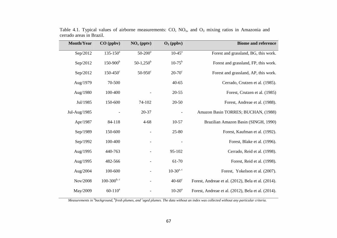
67

Table 4.1. Typical values of airborne measurements: CO, NOx, and O3 mixing ratios in Amazonia and

cerrado areas in Brazil.

Month/Year CO (ppbv)

NOx (pptv) O3 (ppbv) Biome and reference

Sep/2012 135-150a 50-200

a 10-45

a Forest and grassland, BG, this work.

Sep/2012 150-900b 50-1,250

b 10-75

b Forest and grassland, FP, this work.

Sep/2012 150-450c 50-950

c 20-70

c Forest and grassland, AP, this work.

Aug/1979 70-500 40-65 Cerrado, Crutzen et al. (1985).

Aug/1980 100-400 - 20-55 Forest, Crutzen et al. (1985)

Jul/1985 150-600 74-102 20-50 Forest, Andreae et al. (1988).

Jul-Aug/1985 - 20-37 - Amazon Basin TORRES; BUCHAN, (1988)

Apr/1987 84-118 4-68 10-57 Brazilian Amazon Basin (SINGH, 1990)

Sep/1989 150-600 - 25-80 Forest, Kaufman et al. (1992).

Sep/1992 100-400 - - Forest, Blake et al. (1996).

Aug/1995

Aug/1995

440-763

482-566

-

-

95-102

61-70

Cerrado, Reid et al. (1998).

Forest, Reid et al. (1998).

Aug/2004 100-600

- 10-30a, c

Forest, Yokelson et al. (2007).

Nov/2008 100-300b, c

- 40-60c

Forest, Andreae et al. (2012), Bela et al. (2014).

May/2009 60-110a - 10-20

a Forest, Andreae et al. (2012), Bela et al. (2014).

Measurements in abackground, bfresh plumes, and caged plumes. The data without an index was collected without any particular criteria.

68

The O3 mixing ratios in the BG environment reached 40 ppbv at about 600 m altitude

during flight B735 (at 11:30 am, Figure 4.2), although typical values ranged from 10 to

45 ppbv (< 2000 m). This value of 40 ppbv is nearly double the mean value of O3

mixing ratio that we used as background in the enhancement ratio, and even out of the

range of the standard deviation (21 ppbv, SD=7). Bela et al. (2014) reported O3 ranging

from 10 to 20 ppbv during the wet-to-dry transition season (May/June 2009),

measurements performed in a clean atmosphere during the Regional Carbon Balance in

Amazonia (BARCA B) campaign. In contrast, during BARCA A campaign, in the dry-

to-wet transition season (November/December 2008), the O3 mixing ratio ranged from

40 to 60 ppbv in an area influenced by fires, values which are comparable with FP (10-

75 ppbv) and AP (20-70 ppbv), and even in BG conditions (10-45 ppbv) during

SAMBBA.

In terms of CO and NOx, the flight tracks classified as FP were the most polluted of the

campaign. The CO and NOx mixing ratios for FP reached, respectively, values above

3,000 and 60 ppbv at 600 m from the surface between 11:00 am and 12:00 pm. The

enhancement of CO and NOx mixing ratios near the surface suggests an initial vertical

transport due to the hot plume buoyancy, which may increase the tracer lifetime

released to the atmosphere. The vertical transport can be observed mainly for CO at

different altitudes and time of the day since the CO is preserved longer along the plume

when compared with NOx. The measurements in fresh biomass burning plumes also

captured higher levels of CO mixing ratios (500 ppbv) at 1.4 km and 2 km of altitude.

Yokelson et al. (2007), during the Tropical Forest and Fire Emissions Experiment

(TROFFEE), reported a vertical transport mechanism, called a “mega-plume”, at 2km

altitude during a flight in the south of the Amazon rainforest (from Manaus to Cuiabá),

with CO mixing ratio reaching 1,200 ppbv. The TROFFEE experiment used airborne

measurements during the 2004 Amazon dry season, and reported, on 8 September, the

presence of a massive plume formed from numerous fires. During SAMBBA campaign,

we also detected the presence of similar mega-plumes during the flight B742, classified

mostly as FP, with a unique CO mixing ratio value, peaking ~5,000 ppbv at about 600

m. These results demonstrate the strength of vertical transport during a fresh biomass

69

burning event, with the plume injection height up to 2 km. Freitas et al. (2006, 2007,

2010) highlighted the importance of representing the injection height of biomass

burning plumes in numerical models to describe the regional smoke distribution.

Trentmann and Andreae (2003) also demonstrated a large impact of fire emissions on

the chemical composition in a young biomass burning plume using a 3-D chemical

transport model and direct observations. These authors reported simulated high values

near the fire (z 150 m) for CO and NOx, with mean values around 18,000 ppbv and

404 ppbv, respectively. On the other hand, Andreae et al. (2012) reported CO mixing

ratios up to 300 ppbv in a smoky region in the southern Amazon basin during the

BARCA experiment. The highest values were found at about 1,000 m altitude, late in

the dry season (BARCA-A, November 2008). In this study, the CO mixing ratio

measurements in FP and AP ranged from 150 to 900 ppbv and from 150 to 450 ppbv,

respectively. The CO mixing ratios in FP (150-900 ppbv) are comparable with values

found by Reid et al. (1998) in a cerrado area (440-763 ppbv) and some forest studies (up

to 600 ppbv) conducted by Andreae et al. (1988), Kaufman et al. (1992) and Yokelson

et al. (2007). The values found in AP were consistent with values of CO mixing ratios

from forest areas, impacted by haze smoke plumes (Table 4.1).

In Figure 4.2, during most of the flight tracks classified as AP, the NOx mixing ratio

values were below 2 ppbv, except for a peak of 6 ppbv at 600 m from the surface

between 11:30 am and 12:00 pm, a value below that observed in the FP environment

(60 ppbv). On the other hand, the O3 mixing ratio results in AP presented high levels (

80 ppbv) around 12:10 pm at 1,300 m altitude. We also investigated the high levels of

CO and NOx mixing ratios found in FP corresponding to the same flight in which we

also detected high levels of O3 in AP. In fact, Figure 4.3 shows the track of flight B742

in a transition from a remote site impacted by FP to an urban site in Palmas-TO, with

high levels of O3 ( 80 ppbv).

70

Figure 4.3. On the left, the track of flight B742 that landed in Palmas – TO. The color bar is

representing the measured O3 mixing ratios (ppbv) along the flight track. On the right, from top

to bottom, the altitude, and the CO, NOx and O3 mixing ratios (ppbv) measured along the same

flight track. The red and blue dots are representing the parts of the flight track classified as fresh

(FP) and aged (AP) smoke plumes, respectively.


The mean value of O3 found in FP was 31 ppbv (SD = 14), which is 29% lower than

measured for AP (44 ppbv, SD = 13 ppbv), since O3 is produced as a secondary product

from the interaction between VOCs and NOx. The O3 mixing ratios in FP peak at about

60 ppbv near the surface (200–600 m) and, for most cases, plumes with about 40 ppbv

were observed both near the surface and in high altitudes (Figure 4.2). During the

TROFFEE experiment, Yokelson et al. (2007) found O3 mixing ratios of about 30 ppbv

in smoke haze layers in Amazonia. Our results showed higher values for O3 mixing

ratios, ranging from 10 to 75 ppbv in FP and 20 to 70 ppbv in AP. Agreeing with the

SAMBBA results, Reid et al. (1998) found O3 mixing ratios ranging from 60 to 100

ppbv during SCAR-B experiment in 1995 dry season, and Kaufman et al. (1992) found

similar levels of O3 in a forest site in Amazonia during BASE A (Table 4.1).

71

4.2.2. Long-range transport of O3

We analyzed the ozone vertical distribution for all SAMBBA flights following the

methodology proposed by Greenslade et al. (2017). To identify a long-range transport

event, we selected the flights excluding the first 0.5 km of altitude to avoid noise levels

of ozone, characteristic in a region impacted by biomass burning. We also filtered the

data ignoring high O3 events within 0.5 km of the tropopause (> 8 km) to reduce

uncertainties related with the variations in lower stratospheric and upper tropospheric

layer. Then, after calculating the 99th

percentile perturbation value, we separated the

flights using the O3 threshold (83.5 ppbv) as criteria to identify the long-range transport

events.

The O3 is formed photochemically during the smoke plume aging and we used the

enhancement ratio 𝐸𝑅[Δ𝑂3]/[Δ𝐶𝑂] as an indicator of the smoke plume age, according to

the Eq. 3.1. The enhancement ratio 𝐸𝑅𝑂3/𝐶𝑂 allowed us to identify aged plumes

during the analyzes, corroborating the influence of long range transport. Table 3.4 list

values of 𝐸𝑅𝑂3/𝐶𝑂 and the estimated plume age for several measurements in tropical

and subtropical sites.

Figure 4.4.a shows the vertical profile of O3 mixing ratio for all SAMBBA flights and

its approximate plume age through the 𝐸𝑅𝑂3/𝐶𝑂. The high values of O3 mixing ratio

(> 83.5 ppbv) found between 5,500 and 6,500 m of altitude, also presented high values

for the enhancement ratio (𝐸𝑅𝑂3/𝐶𝑂 > 2), suggesting long-range transport of ozone.

We detected two possible long-range ozone transport events between 5,500 – 6,500 m

of altitude (O3 > 83.5 ppbv), southward (flights B744 and B745) and westward (flight

B746) from Porto Velho – RO. These scientific flights affected by long-range transport

occurred on September 24 and 29, 2012 (Figure 4.4.b).

During this same period, the O3 product retrieved from Atmospheric Infrared Sounder

(AIRS) measurements onboard the AQUA satellite during daytime highlights the long-

range ozone transport from biomass burning emissions in Africa, with an inflow into the

Amazon basin at 500 hPa (Figure 4.5).

72

Figure 4.4. (a) Vertical profiles of O3 with the altitude and as a function of ER𝑂3/𝐶𝑂 (color

scale) for all SAMBBA flights. (b) Flights identified as a long-range transport of ozone.


Figure 4.5. Time averaged Ozone (ppmv) from September 24 to 29 2012 retrieved from AIRS

onboard AQUA satellite during daytime at 500 hPa, with 1º x 1º spatial resolution.

Source: Adapted from AIRS.

73

4.2.3. Isoprene and its oxidation ratio

Information about the isoprene transport and chemistry can be derived from the isoprene

abundance in the atmosphere and the ratio of its oxidation products relative to isoprene,

[MVK+MACR+ISOPOOH]/[isoprene]. During the day, the isoprene chemistry is

affected mainly by the distance from the emission source (transport time),

photochemical degradation and availability of OH, which reacts with isoprene to

produce chemical species including MVK, MACR and ISOPOOH (KUHN et al., 2007;

LIU et al., 2016). During SAMBBA, the mean isoprene mixing ratio in BG was 2.8

ppbv and 1.5 ppbv for the boundary layer and free troposphere, respectively. We also

detected higher values of O3 (40 ppbv at 600 m) in BG, shown in Figure 4.2, coinciding

with the interpolated cross section of the isoprene (4 ppbv at 600 m), also in BG

environment (Figure 4.6). As mentioned by Barket et al. (2004), in fact, a sequence of

reactions initialized by the reaction of isoprene with OH leads to the production of

organic peroxy radicals (RO2), that then react with NOx promoting the ozone formation

observed during the BG flights tracks. Table 4.2 summarizes the mean values of

isoprene and the oxidation ratio [MVK+MACR+ISOPOOH]/[isoprene] during

SAMBBA, together with previously-reported airborne measurements in remote areas

and biomass burning environments. The isoprene mixing ratios measured during

SAMBBA in BG environment generally agree with values reported in pristine areas of

the Amazon forest (Greenberg et al., 2004; Greenberg and Zimmerman, 1984; Gregory

et al., 1986; Helmig et al., 1998; Kuhn et al., 2007; Lelieveld et al., 2008; Rasmussen

and Khalil, 1988; Zimmerman et al., 1988). Some studies conducted in the Amazonian

tropical forest, e.g., Greenberg et al. (2004) and Kuhn et al. (2007), have higher

isoprene with reported values up to ~6 to 7 ppbv.

74

Figure 4.6. Cross section of the isoprene mixing ratio (ppbv) (top) and the [MVK+MACR+ISOPOOH]/[Isoprene] ratio (bottom) for the three

different groups: background environment (on the left), fresh smoke plume (t < 2 hours, in the middle), and aged smoke plume (t > 2 hours, on the

right). The aircraft data was interpolated from the various vertical profile measurements using kriging correlation method. White dashed lines show

the flight tracks. Hour is presented in local time.


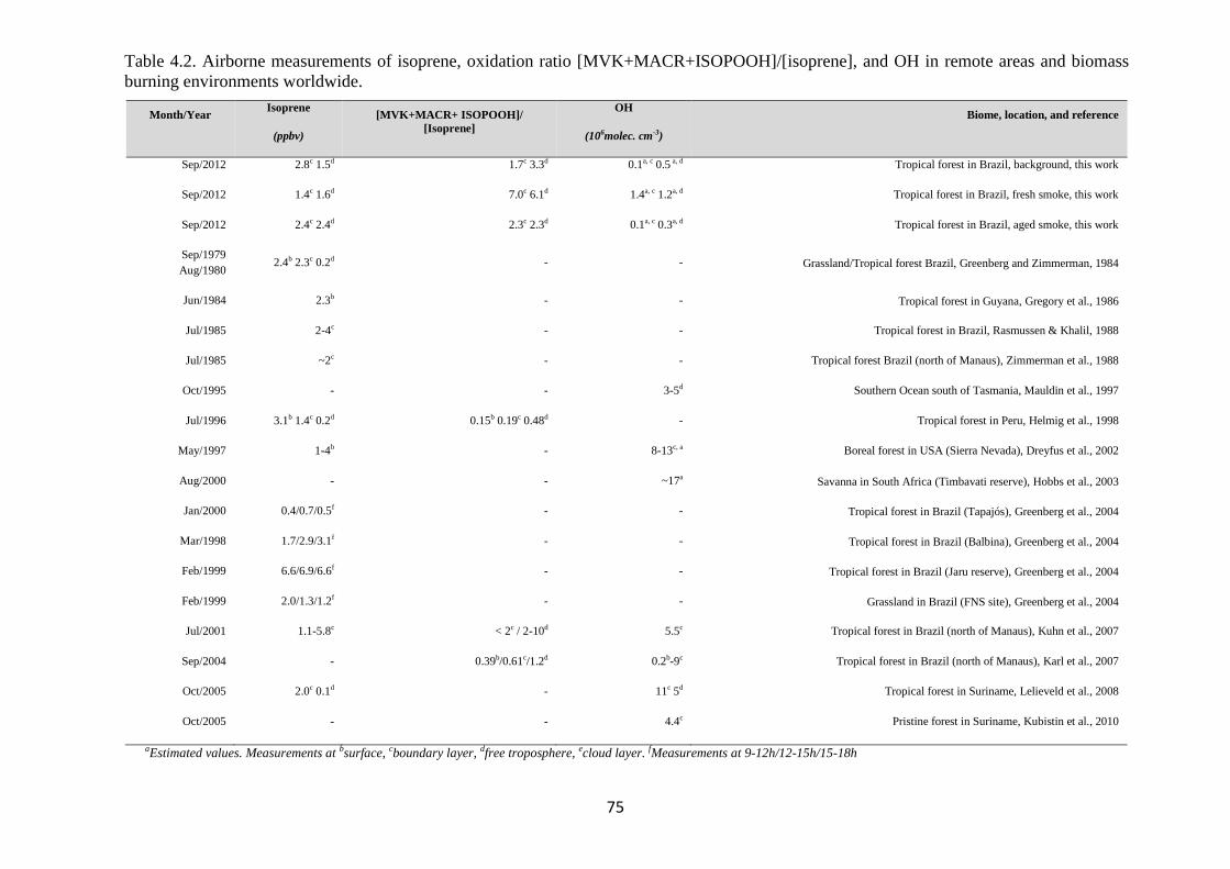
75

Table 4.2. Airborne measurements of isoprene, oxidation ratio [MVK+MACR+ISOPOOH]/[isoprene], and OH in remote areas and biomass

burning environments worldwide.

Month/Year

Isoprene

(ppbv)

[MVK+MACR+ ISOPOOH]/

[Isoprene]

OH

(106molec. cm-3)

Biome, location, and reference

Sep/2012 2.8c 1.5d 1.7c 3.3d 0.1a, c 0.5 a, d Tropical forest in Brazil, background, this work

Sep/2012 1.4c 1.6d 7.0c 6.1d 1.4a, c 1.2a, d Tropical forest in Brazil, fresh smoke, this work

Sep/2012 2.4c 2.4d 2.3c 2.3d 0.1a, c 0.3a, d Tropical forest in Brazil, aged smoke, this work

Sep/1979

Aug/1980 2.4b 2.3c 0.2d - - Grassland/Tropical forest Brazil, Greenberg and Zimmerman, 1984

Jun/1984 2.3b - - Tropical forest in Guyana, Gregory et al., 1986

Jul/1985 2-4c - - Tropical forest in Brazil, Rasmussen & Khalil, 1988

Jul/1985 ~2c - - Tropical forest Brazil (north of Manaus), Zimmerman et al., 1988

Oct/1995 - - 3-5d Southern Ocean south of Tasmania, Mauldin et al., 1997

Jul/1996 3.1b 1.4c 0.2d 0.15b 0.19c 0.48d - Tropical forest in Peru, Helmig et al., 1998

May/1997 1-4b - 8-13c, a Boreal forest in USA (Sierra Nevada), Dreyfus et al., 2002

Aug/2000 - - ~17a Savanna in South Africa (Timbavati reserve), Hobbs et al., 2003

Jan/2000 0.4/0.7/0.5f - - Tropical forest in Brazil (Tapajós), Greenberg et al., 2004

Mar/1998 1.7/2.9/3.1f - - Tropical forest in Brazil (Balbina), Greenberg et al., 2004

Feb/1999 6.6/6.9/6.6f - - Tropical forest in Brazil (Jaru reserve), Greenberg et al., 2004

Feb/1999 2.0/1.3/1.2f - - Grassland in Brazil (FNS site), Greenberg et al., 2004

Jul/2001 1.1-5.8c < 2c / 2-10d 5.5c Tropical forest in Brazil (north of Manaus), Kuhn et al., 2007

Sep/2004 - 0.39b/0.61c/1.2d 0.2b-9c Tropical forest in Brazil (north of Manaus), Karl et al., 2007

Oct/2005 2.0c 0.1d - 11c 5d Tropical forest in Suriname, Lelieveld et al., 2008

Oct/2005 - - 4.4c Pristine forest in Suriname, Kubistin et al., 2010

aEstimated values. Measurements at bsurface, cboundary layer, dfree troposphere, ecloud layer. fMeasurements at 9-12h/12-15h/15-18h

76

On average, we found lower isoprene in FP (1.4 ppbv), and slightly lower in AP (2.4

ppbv), relative to the BG value (2.8 ppbv), within the PBL (<1,200 m), around 50% and

14%, respectively.

In contrast, above the PBL (> 1,2000 m) we observed a substantial increase of about

60% of the isoprene in AP (2.4 ppbv) relative to the BG value (1.5 ppbv), which is

about the same mean value found in FP (1.6 ppbv). These high levels of isoprene at

higher altitudes in air masses affected by biomass burning emissions, are likely to be

associated with the heat released from vegetation fires affecting nearby plants that also

release significant amounts of isoprene to the atmosphere, especially in tropical forest

fires in Brazil (Ciccioli et al., 2014). Müller et al. (2016), for example, found isoprene

mixing ratios up to 15 ppbv in a smoke plume from a small forest understory fire in

Georgia, USA. We also found higher isoprene mixing ratios in upper levels (> 1,200 m)

in smoke areas when compared with pristine mixed layer studies mentioned previously.

These results reinforce the hypothesis that fire activity promoted the isoprene transport

to higher altitudes both in fresh ( 6 ppbv, 1,700–2,000 m) and aged plumes ( 4 ppbv,

1,600–2,000 m) during SAMBBA flights (Figure 4.6). In Figure 4.7, we also verified

the average isoprene mixing ratio (< 2,000 m) in AP (2.4 ppbv) was 71% higher than FP

(1.4 ppbv) and similar to the mean value measured in BG (2.6 ppbv).

In fresh smoke plumes, biomass burning tracers, such as acetonitrile and acetaldehyde,

are present at a relatively high concentration, while the [MVK+MACR+

ISOPOOH]/[isoprene] ratio is low. In contrast, aged smoke plumes typically have

higher values for the [MVK+MACR+ISOPOOH]/[isoprene] ratio, since there is more

time for the isoprene to degrade. Figure 4.8 presents the plume interception during the

flight B732, between 10:00 am and 11:30 am, in which it is possible to observe the

difference between FP and AP interceptions through the biomass burning tracers and

[MVK+MACR+ISOPOOH]/[isoprene] ratio. In this study, we found the

[MVK+MACR+ISOPOOH]/[isoprene] ratio mean value ranging from around 1.7 in the

boundary layer to 3.3 in the free troposphere for BG conditions, with AP presenting a

similar value (2.3) for both boundary layer and free troposphere.

77

Figure 4.7. Isoprene, acetonitrile and carbon monoxide mixing ratios (ppbv) as function of the

daytime (local time) for the different chemical regimes previously classified as background

(green dots), smoke fresh plume (red dots), and aged smoke plume (blue dots). Black dash lines,

and the numbers next to them, are representing the mean values of the measurements taken

below 2,000 m of altitude. Hour is presented in local time (11:00 – 18:00 h).


In contrast, FP had the highest value in the boundary layer (7.0) and free troposphere

(6.1), similar to values reported by Kuhn et al. (2007), in the tropical forest in Brazil

(north of Manaus). Above the PBL, we did not find any substantial variation in

[MVK+MACR+ISOPOOH]/[isoprene] ratio associated with the presence of smoke in

AP (2.8), but an increase in the BG value (3.3) in the upper levels (> 1,200 m). The FP

seems to be more active within the boundary layer than at upper levels, with the

isoprene oxidation ratio about 6.1 above 1,200 m. Comparable with our results in FP,

Kuhn et al. (2007), during the Cooperative LBA Airborne Regional Experiment (LBA-

CLAIRE-2001) also found [MVK+MACR+ISOPOOH]/[isoprene] ratio values up to 2,

below 1,000 m of altitude, and between 2 and 10, within the 1,000–2,000 m vertical

layer.

78

Figure 4.8. Methanol (green dots), acetonitrile (orange dots), and acetaldehyde (blue

dots) mixing ratios (ppbv), and the [MVK+MACR+ISOPOOH]/[Isoprene] ratio (gray

bars), during a plume interception along the flight track B732 in different altitudes.


In summary, we found a strong increase in the isoprene oxidation ratio from surface to

2,000 m for FP relative to the BG and AP observed during SAMBBA, similar to other

previous studies in biomass burning environments (Table 4.2).

We observed values of the [MVK+MACR+ISOPOOH]/[isoprene] ratio above 6 in BG

above 1,800 m and between 12:00 pm and 13:30 pm. In contrast, in FP and AP, values

in the range 4-6 are equally distributed in the vertical (Figure 4.6). Along the cloud

layer (1,200–2,000 m), we found that the isoprene oxidation in BG environment tends

to increase (94%) as in AP levels (Table 4.2). Karl et al. (2007) also reported evidence

of an increase of the oxidizing power of the atmosphere in the transition from PBL to

cloud layer (1,200–1,900 m) during TROFFEE experiment, with the

[MVK+MACR+ISOPOOH]/[isoprene] ratio ranging from 0.39 up to 1.2 between 300

m and 1,800 m, already into the cloud layer (CL). Although lower values for the

[MVK+MACR+ISOPOOH]/[isoprene] ratio were found during TROFFEE compared

79

with LBA-CLAIRE, both studies have suggested the occurrence of an oxidizing power

in the transition from the PBL to the CL. In both cases, there was a positive gradient,

increasing the [MVK+MACR+ISOPOOH]/[isoprene] ratio in the CL. Furthermore,

Helmig et al. (1998) reported similar behavior in a remote Peruvian Amazonia site, with

the [MVK]/[isoprene] ratio equal to 0.15, 0.19, and 0.48, near the surface ( 2 m), in the

PBL (91–1,167 m), and above the PBL (1,481–1,554 m) respectively. The

[MVK+MACR+ISOPOOH]/[isoprene] ratio increasing toward the top of the PBL and

CL is likely to be due to the enhancement of the photolysis rates. Direct experimental

data reported by Mauldin et al. (1997) also indicated significant changes above and

inside cloud decks due to cloud edge effects on photolysis rates that have a major

impact on OH production rates. Figure 4.9 presents the density distribution for the

[MVK+MACR+ISOPOOH]/[isoprene] ratio along several altitude layers during

SAMBBA. In FP, the average [MVK+MACR+ISOPOOH]/[isoprene] ratio was equal to

6.3 at 500–1,000 m, 7.6 at 1,000–1,500 m, and returning to 5.9 at 1,500–2,000 m. These

results are consistent with the increase of the oxidative capacity in the transition from

the PBL to the CL, reported by Mauldin et al. (1997) and Karl et al. (2007), with the

SAMBBA measurements showing average [MVK+MACR+ISOPOOH]/[isoprene] ratio

constantly increasing in BG and the highest value at 500 – 1,000 m in AP. The results

showed the isoprene oxidation reaction is enhanced at higher altitudes in the BG

environment, increasing from 1.4 at the first 500 m to 3.4 at 2,000 m.

80

Figure 4.9. Density distributions of the ratio [MVK+MACR+ISOPOOH]/[isoprene], at the

altitude layers (a) 1,500 - 2,000 m, (b) 1,000 - 1,500 m, (c) 500 - 1,000 m and (d) 0 - 500 m. The

Kernel analysis was carried out considering the classification for background (BG), aged smoke

(AP), and fresh smoke plumes (FP). The number of samples and mean values for each group

are depicted near the color bars.


81

4.2.4. OH estimated using the sequential reaction approach

The abundance of OH in the atmosphere is determined by a balance of its production

and loss. Due to the absence of OH measurements during SAMBBA, we inferred the

OH concentrations using a sequential reaction model with the observed profiles of the

[MVK+MACR+ISOPOOH]/[Isoprene] ratio. Table 4.2 presents the average values of

estimated OH concentration in the PBL and CL for the sequential reaction model

approaches of Karl et al. (2007) and the modified approach proposed in this study. In

FP, the estimated OH concentration reached the highest value within the PBL (1.4 x 10-6

molecules cm-3

), when compared with AP or even for the BG environment, both with

OH concentration ~0.1 x 10-6

molecules cm-3

. The photochemical environment in young

biomass burning plumes differs considerably from the clean conditions, especially near

the surface. Hobbs et al. (2003) found OH concentrations of about 1 x 10-7

molecules

cm-3

for a fresh plume from a savanna fire in South Africa, a value higher than found in

our estimation. In CL, the estimated OH in FP reduced to 15% relative to the BG (0.5 x

10-6

molecules cm-3

) environment, in contrast to the increased pattern in AP (0.3 x 10-6

molecules cm-3

).

Figure 4.10 shows the vertical profile of estimated OH concentration in different

chemical regimes, comparing the sequential reaction model according to the original

approach of Karl et al. (2007) with the new approach used in this work. Throughout the

entire altitude range (0 – 2,000 m), the difference in OH calculation between the two

methods was approximately 2 orders of magnitude, although presenting a similar

pattern in the different chemical regimes. Flight tracks classified as BG tend to increase

the OH concentration along the altitude, with the inflection point occurring before the

1,000 m. Differing from BG environments, FP present a decreasing OH concentration

above 1,000 m of altitude, with the AP in an intermediate state. In the flights tracks

classified as BG, we observed the widest variation in the average OH concentration

using the revised sequential reaction model (Figure 4.10, on bottom), especially in

upper levels (5 – 1 x 106 molecules cm

-3), although these results are associated with

higher uncertainties due to a reduced number of samples. In all three different chemical

regimes, the vertical profile of OH concentration presented an increase near to CL

82

(~1,000 m), in agreement with previous studies (MAULDIN et al., 1997; LANGFORD

et al., 2005; KARL et al., 2007; KUHN et al., 2007).

Figure 4.10. Vertical profile of OH concentration (molecules cm-3

) for the different chemical

regimes: background environment (BG), fresh smoke plume (FP), and aged smoke plume (AP).

On top, the sequential reaction model according to the original approach of Karl et al. (2007),

and on bottom, the new approach used in this work. Blues lines are the trend lines and grey

interval represents the level of confidence (0.95) used.


In terms of absolute values, the estimated OH concentration values presented in this

study agree within an order of magnitude with most of the observational values

previously reported for Amazonia and other forest areas. For example, prediction

studies conducted by Warneke et al. (2001) estimated the concentration of OH around

1-3 x 105 molecules cm

-3 (24 h average), and Williams et al. (2001) found a range of

0.6-1.1 x 106 molecules cm

-3 during day daytime. During the Guyanas Atmosphere-

Biosphere exchange and Radicals Intensive Experiment with a Learjet (GABRIEL)

experiment, the average OH concentrations in the boundary layer (<1 km) over the

83

Suriname rainforest in the afternoon was 4.4 x 106 molecules cm

-3 (KUBISTIN et al.,

2010). Dreyfus et al. (2002) reported high levels of OH concentration (3-5 x 106

molecules cm-3

) in the free troposphere over a forest area in Sierra Nevada, California.

4.3. Model coupling: BRAMS+MEGAN

In this section, we present the modeling results for isoprene and OH from the two

experiments using the MEGAN model online and off-line with BRAMS during

SAMBBA, as described in section 3.3.

Figure 4.11 presents the average emissions of isoprene for two settings of the BRAMS

model, BRAMS-MEGAN off-line (a) and BRAMS-MEGAN online (b). BRAMS-

MEGAN off-line during SAMBBA period. BRAMS-MEGAN off-line presented low

values (10-150 µg m-2

day-1

) for isoprene emission in the southeast part of the Amazon

basin, with the highest values (peaking 1,500 µg m-2

day-1

) in the central and west part.

On the other hand, simulations using BRAMS-MEGAN online showed low levels of

isoprene emissions when compared with off-line configuration, typically ranging from

10 – 300 µg m-2

day-1

. The BRAMS-MEGAN online results are comparable with the

most recent isoprene emission estimates from aircraft eddy covariance measurements

over the Amazonian forest (GU et al., 2017), close to 200 mg m-2

day-1

. Some

discrepancy in the results can be related with the assumption that grid domain has the

same PFT (broadleaf evergreen tropical tree) in the settings of BRAMS-MEGAN

online, impacting in the results of southeast part of Amazon basin.

Figure 4.12 show the time series of isoprene mixing ratio in the first model layer (~40 m

de altitude) between 14 September and 03 October 2012. The isoprene from BRAMS-

MEGAN online has a diurnal cycle varying from 1 to 10 ppbv, which is the same order

of magnitude of the isoprene levels measured at the K-34 tower and reported in previous

studies (KARL et al., 2007; KUHN et al., 2007; YÁÑEZ-SERRANO et al., 2015). On

the other hand, BRAMS-MEGAN off-line tends to overestimate the isoprene mixing

ratio near the top of the canopy. Moreover, the overestimation of the isoprene as

predicted by BRAMS-MEGAN off-line occurs not only during the daytime. The lower

84

values of isoprene mixing ratio during the nighttime are around 10 ppbv, which is up to

five times higher than the values typically observed in Amazonia during this time of the

year (YÁÑEZ-SERRANO et al., 2015). Therefore, the results of the coupled model are

improved not only regarding the mean daily values of isoprene mixing ratio but also

regarding the diurnal cycle, ranging from 3 to 12 ppbv during the daytime and 0.5 to 3

ppbv during the nighttime.

Figure 4.11. Average isoprene emissions rate from the model simulations during the SAMBBA

period from 14 September to 03 October 2012: (a) Off-line BRAMS-MEGAN and (b) Online

BRAMS-MEGAN.


Figure 4.13 represents the mean diurnal cycle of isoprene mixing ratio at the first model

layer from the two model simulations during SAMBBA at the K-34 tower. In average,

the isoprene mixing ratio from the off-line model peaks 20 ppbv around 12 UTC (9:00

local time). In addition, the off-line model results are offset for about 3 hours compared

to the online model results. Previous measurements in Amazonia towers showed that the

isoprene tend to peak around 2 – 8 ppbv between 13-17 local time, depending on the dry

or wet season (KARL et al., 2007; KUHN et al., 2007; YÁÑEZ-SERRANO et al.,

2015). Therefore, the online model also corrects the diurnal cycle of the isoprene

mixing ratio at the top of the canopy.

Isopren

e [mg

m-2

day

-1]

(a) (b)

85

Figure 4.12. Time series of the isoprene mixing ration (ppbv) from the numerical simulations

during SAMBBA field campaign in the tower K-34 site at the first model vertical layer. Black

line represents BRAMS-MEGAN off-line and green lines BRAMS-MEGAN coupled online.


Figure 4.13. Mean diurnal cycle of isoprene mixing ratio from the model simulations at the K-

34 tower during the SAMBBA period from 14 September to 03 October 2012.


Iso

pre

ne [

pp

bv

]

-5

0

5

10

15

20

25

30

0 3 6 9 12 15 18 21 24

Isop

rene [

pp

bv]

Hour [UTC]

BRAMS-MEGAN online BRAMS-MEGAN offline

86

The isoprene emission depends of several factors, such as LAI, solar radiation,

temperature, moisture, CO2, and source type (Plant Functional Type and the

corresponding Emission Factor). To assess the factors that influence the isoprene

concentration patterns near the surface, we opted for the Pearson correlation analysis for

each version of the numerical model BRAMS. Table 4.3 shows the main factors that

drive the isoprene emissions in MEGAN model. For light dependent emissions,

MEGAN includes a light response that is based on electron transport (Guenther et al.,

1991), a temperature response based on enzymatic activity (Guenther et al., 1991), and

an inhibition response for CO2 based on changes in metabolite pools, enzyme activity,

and gene expression (Wilkinson et al., 2009). As expected, the isoprene from the

simulation of the BRAMS-MEGAN online presented a high correlation with the short-

wave radiation (0.95), surface temperature (0.62), and, a negative correlation with CO2.

On the other hand, the isoprene from the BRAMS-MEGAN off-line does not respond to

the MEGAN dependence basic formulation of isoprene emissions with the

aforementioned variables (Table 4.3) and therefore constitutes a limitation.

Table 4.3. Pearson correlation coefficient before and after BRAMS-MEGAN

coupling.

Isoprene

Pearson correlation coefficient

CO2 Surface

temperature

Short-wave

radiation

BRAMS-MEGAN off-line 0.37 -0.34 -0,16

BRMAS-MEGAN online -0.42 0.62 0.95

Even near the surface, the isoprene concentration depends not only on the isoprene

emissions, several other chemical compounds and the air masses transport can also alter

its concentration. With the aim to investigate the impact of polluted areas surrounding

forest areas in Amazon basin, also sought to compare pristine regions with those

87

impacted by anthropogenic emissions, either by burning sources or by urban emissions.

Figure 4.14 presents the number of fires detected from MODIS onboard AQUA during

SAMBBA field campaign. We selected two sectors (1 and 2) located, respectively, in

clean and polluted areas to assess the impact of biomass burning emission on isoprene

levels. Important to note that both sectors have the isoprene emissions ranging between

100 and 150 µg m-3

h-1

in the online model setting. On contrast, the emissions for the

off-line model are typically around 300 µg m-3

h-1

in sector 1, and ranging between 300

and 1,500 µg m-3

h-1

in sector 2. So, when comparing the isoprene concentrations in

these two sectors, must keep in mind that the differences are not only related with

biomass burning emissions but also with the differences in terms of model

representation of the biogenic emissions itself. In fact, the time series of isoprene

mixing ratios in sectors 1 and 2, according to the online and off-line models, reflect

these differences (Figure 4.15). The off-line model in polluted region resulted in values

for isoprene mixing ration near surface about twice higher than in clean region, which

was already overestimated. On the other side, the online resulted on value for the

isoprene mixing ratio in sector 1 only slightly above the values in sector 2 on specific

days. The results of the online model are consistent with the magnitude of the isoprene

mixing ratios observed during SAMBBA and previous studies.

88

Figure 4.14. Selected sectors based on number of fires detected from MODIS onboard AQUA

during SAMBBA campaign in 2012.

Source: Adapted from https://queimadas.dgi.inpe.br/. Accessed on 05 April 2017

Figure 4.15. Time series of the isoprene mixing ratio from the numerical simulations during

SAMBBA field campaign in clean and polluted area (see Figure 4.14) at the first model vertical

layer.


Number of fires detected

September 2012

AQUA (morning/afternoon)

Size of the squares ~25km x 25km

Manaus

Porto Velho

Sector 1

Sector 2

Isop

rene [

pp

bv

]

89

Figure 4.16. Vertical profile of the isoprene mixing ration from the numerical simulations

during SAMBBA field campaign in clean and polluted area (see Figure 4.14).


Figure 4.17 show the time series of OH mixing ratio in the first model layer (~40 m de

altitude) between 14 September and 03 October 2012. In general, BRAMS-MEGAN

online presented higher values for OH than BRAMS-MEGAN off-line during the

SAMBBA field campaign. This pattern was evident during the last days, 28 September

to 4 October, with a difference of up to one order of magnitude. BRAMS-MEGAN off-

line presented values of OH close those estimated in fresh smoke plumes (1.5 x 106

molecules cm-3

) and higher than aged smoke plumes (5 x 105 molecules cm

-3) in

SAMBBA.

Isoprene [ppbv]

Alt

itud

e [m

ete

rs]

90

Figure 4.17. Time series of the OH mixing ratio from the numerical simulations during

SAMBBA field campaign in clean and polluted area (see Figure 4.14) at the first model vertical

layer.

Figure 4.18 shows the OH vertical profile up to 1200 m altitude for BRAMS-MEGAN

online and offline configurations. BRAMS-MEGAN online showed high values along

the vertical profile when compared to BRAMS-MEGAN off-line, achieving an OH

concentration of ~3 x 107 molecules cm

-3 at 1,200 m of altitude.

This observed increase in OH near to 1,100 – 1,200 meters of altitude, both in the online

and offline model, was also detected in the OH estimated in a fresh smoke plume and

clean area environment. In all three different chemical regimes, the vertical profile of

estimated OH also presented an increase near to the cloud layer, in agreement with

model results and previous studies (MAULDIN et al., 1997; LANGFORD et al., 2005;

KARL et al., 2007; KUHN et al., 2007).

OH

[m

ole

cule

s cm

-3]

91

Figure 4.18. Vertical profile of the OH mixing ratio from the numerical simulations during

SAMBBA field campaign in clean and polluted area (see Figure 4.14).

Alt

itu

de

[mete

rs]

OH [molecules cm-3 ]

92

93

5 CONCLUSIONS

We present a concise chemical characterization of the atmosphere of Brazilian

Amazonia during the SAMBBA airborne experiment from 14th

September to 3rd

October 2012, comprising the transition period from the dry to wet season. The flights

were carried out in remote areas, as well as areas under the influence of biomass

burning that commonly occurs in the region. The flight classification method adopted in

this study prioritized the chemical classification, using CO mixing ratios and the

enhancement ratio of O3 to CO to categorize different flight tracks to include BG

flights, and FP and AP flights.

Measurements of CO, NOx, and O3 performed in areas not directly affected by local fire

emissions reveals the signature of biomass burning in the chemical composition of the

background of the Amazonian atmosphere, due to long-range transport of biomass

burning tracers both from Africa and the eastern part of Amazonia. The CO and O3

mixing ratios exceeded the background values reported in other studies. Satellite-

derived data, however, indicate there was a significant inflow of smoke tracer from

Africa. Corroborating previous studies (AZEVEDO et al., 2010; LANGFORD et al.,

2010; SRIVASTAVA; NAJA; THOURET, 2015), we found evidence of long-range

transport events of O3 during SAMBBA experiment, considering the high levels of O3

in aged plumes at high altitudes (5,500 – 6,500 m), and the AIRS detection of an O3

inflow in the Amazon basin from Africa. These findings support the hypothesis that the

long-range transport events can be an important source of O3 into the troposphere in the

Amazon basin, which could even alter the atmospheric composition within the planetary

boundary layer. We also emphasize the importance of further studies about the long-

range ozone transport in the southern hemisphere, focusing on long-term records of

vertical ozone profile to reduce the uncertainty especially related with seasonality and

representativeness of the SAMBBA measurements.

In our analysis, we highlight the importance of photochemical age in areas influenced

by biomass burning emission, with distinct results for FP and AP. Fresh smoke plumes

had the highest mixing ratios of CO and NOx, showing up the strength of vertical

94

transport through the detection of biomass burning products in upper levels (> 1,200 m).

In AP, we detected up to 80 ppbv of O3 at 1,300 m altitude, showing the O3 levels in the

transition from a remote site impacted by fresh smoke plumes to an urban site in

Palmas-TO.

Regarding isoprene, we showed that there is an indication of the heat released from

vegetation fires affecting the nearby plants which consequently also significantly

increases amount of isoprene released to the atmosphere especially in AP environment.

In contrast with BG condition (1.5 ppbv), the isoprene mixing ratio in AP was 2.4 ppbv

in the free troposphere, followed by 1.6 ppbv in FP. The FP also presented a higher

[MVK+MACR+ISOPOOH]/[isoprene] ratio (7.0), when compared with both AP (2.3)

and BG (1.7), indicating a strong oxidation process within the boundary layer.

Improving the simplified sequential reaction model used by Karl et al. (2007), we

indirectly calculated the OH concentration in different chemical regimes and the results

are comparable with observations. The highest value for OH in FP within the PBL (1.4

x 10-6

molecules cm-3

) corroborate the results from

[MVK+MACR+ISOPOOH]/[isoprene] ratio, confirming that the photochemical

environment in young biomass burning plumes differs considerably from background

conditions. We also detected the strong signal in the oxidative capacity at higher levels

(~1,000 m), characteristic of the cloud layer existence, as reported by others studies

(MAULDIN et al., 1997; KARL et al., 2007).

Looking for a synergistic analysis between observations and numerical modeling, a

coupling of the MEGAN model was developed in the numerical model BRAMS. The

coupled model was able to reproduce the typical diurnal concentrations of isoprene on

the surface, including corrections in the period of emission. Improvements were also

observed in the isoprene concentrations at night, with values close to those obtained in

recent observation studies in the Amazonian basin. Corroborating the improvement in

the isoprene simulation, BRAMS-MEGAN online presented the expected correlation

with the short-wave radiation, surface temperature, and a negative correlation with CO2

during SAMBBA field campaign. Although the new version of the BRAMS model

performed well in the simulations of the isoprene concentration, the model did not agree

95

with the estimated and observed results for OH. More tests are needed to investigate the

possible causes of disagreement between the model result and the observations and

estimates presented here. However, the results of the model also showed the influence

of the cloud layer on increasing the oxidative capacity, as predicted in the estimated OH

calculations.

In this thesis, we observed an improvement in the estimated OH concentration values

using the modified sequential reaction model described in the section 3.1.4, for both

biomass burning regimes and background environment. Both methods, column and

plume approach, are useful to estimate the OH and some discrepancies may be

associated with uncertainties in dynamic factors in the simplified analytical expression,

such as vertical and horizontal transport, convective velocity above different vegetation

cover, as well as the radiation regime influenced by clouds at high altitudes which are

likely to affect the OH concentrations. We also assessed the impact of the model

improvement in isoprene concentration and OH modeled, with a reasonable agreement

for isoprene concentration and more investigation needed for the OH simulation.

The findings corroborate the influence of biomass burning activity not only on direct

emissions of particulate matter, but also in the oxidative capacity to produce secondary

organic aerosol through the gas-particle conversion that occurs in the atmosphere. The

author highlights the potential use of the research results to improve the numerical

model simulation with a better representativeness of the chemistry processes, which can

impact on the global climate prediction.

For future studies, we recommend further investigation of the impact of the dynamic

factors, such as horizontal transport, convective velocity above different vegetation

cover, in the estimation of OH mixing ratios, as well as the effect of the radiation

regime influenced by clouds at high altitudes altering photolysis rates. Considering the

recent updates in the oxidative capacity of the atmosphere, we also expect a reduction in

the uncertainties associated with the OH concentrations.

96

97

REFERENCES

AGHEDO, A. M.; SCHULTZ, M. G.; RAST, S. The influence of African air pollution

on regional and global tropospheric ozone. Atmospheric Chemistry and Physics, v. 7,

p. 1193–1212, 1 jan. 2007.

ALONSO, M. F.; LONGO, K. M.; FREITAS, S. R.; MELLO DA FONSECA, R.;

MARÉCAL, V.; PIRRE, M.; KLENNER, L. G. An urban emissions inventory for South

America and its application in numerical modeling of atmospheric chemical

composition at local and regional scales. Atmospheric Environment, v. 44, n. 39, p.

5072–5083, 2010.

ANDREAE, M. O.; ANDERSON, B. E.; BLAKE, D. R.; BRADSHAW, J. D.;

COLLINS, J. E.; GREGORY, G. L.; SACHSE, G. W.; SHIPHAM, M. C. Influence of

Plumes from Biomass Burning on Atmospheric Chemistry over the Equatorial and

Tropical South-Atlantic during Cite-3. Journal of Geophysical Research-

Atmospheres, v. 99, n. D6, p. 12793–12808, 1994a.

ANDREAE, M. O.; ANDERSON, B. E.; BLAKE, D. R.; BRADSHAW, J. D.;

COLLINS, J. E.; GREGORY, G. L.; SACHSE, G. W.; SHIPHAM, M. C. Influence of

plumes from biomass burning on atmospheric chemistry over the equatorial and tropical

South Atlantic during CITE 3. Journal of Geophysical Research, v. 99, n. 94, p. 0–1,

1994b.

ANDREAE, M. O.; ARTAXO, P.; BECK, V.; BELA, M.; FREITAS, S.; GERBIG, C.;

LONGO, K.; MUNGER, J. W.; WIEDEMANN, K. T.; WOFSY, S. C. Carbon

monoxide and related trace gases and aerosols over the Amazon Basin during the wet

and dry seasons. Atmospheric Chemistry and Physics, v. 12, n. 13, p. 6041–6065,

2012.

ANDREAE, M. O.; GARSTANG, M.; GREGORY, G. L.; HARRISS, R. C.;

PEREIRA, M. C.; SACHSE, G. W.; SETZER, A. W.; TALBOT, R. W.; TORRES, A.

L.; WOFSY, S. C. Biomass-Burning Emissions and Associated Haze Layers Over

Amazonia. Journal of Geophysical Research, v. 93, p. 1509–1527, 1988.

ARNETH, A.; SCHURGERS, G.; LATHIERE, J.; DUHL, T.; BEERLING, D. J.;

HEWITT, C. N.; MARTIN, M.; GUENTHER, A. Global terrestrial isoprene emission

models: Sensitivity to variability in climate and vegetation. Atmospheric Chemistry

and Physics, v. 11, n. 15, 2011.

ARTAXO, P.; RIZZO, L. V; BRITO, J. F.; BARBOSA, H. M. J.; ARANA, A.; SENA,

E. T.; CIRINO, G. G.; BASTOS, W.; MARTIN, S. T.; ANDREAE, M. O. Atmospheric

aerosols in Amazonia and land use change: from natural biogenic to biomass burning

conditions. Faraday Discussions, v. 165, p. 203–235, 2013.

AUMANN, H. H.; MILLER, C. C. R. C. Atmospheric infrared sounder (AIRS) on the

98

Earth Observing System. In: SATELLITE REMOTE SENSING II, 15 dez. 1995,

Anais... SPIE, 15 dez. 1995Disponível em:

<http://proceedings.spiedigitallibrary.org/proceeding.aspx?articleid=1008572%5Cnhttp:

//link.aip.org/link/?PSISDG/2583/332/1>

AZEVEDO, J. M.; GON?ALVES, F. L. T.; DE F?TIMA ANDRADE, M.;

GONÇALVES, F. L. T.; DE FÁTIMA ANDRADE, M. Long-range ozone transport and

its impact on respiratory and cardiovascular health in the north of Portugal.

International Journal of Biometeorology, v. 55, n. 2, p. 187–202, 1 jul. 2010.

BARKET, D. J.; GROSSENBACHER, J. W.; HURST, J. M.; SHEPSON, P. B.;

OLSZYNA, K.; THORNBERRY, T.; CARROLL, M. A.; ROBERTS, J.; STROUD, C.;

BOTTENHEIM, J.; BIESENTHAL, T. A study of the NOx dependence of isoprene

oxidation. Journal of Geophysical Research D: Atmospheres, v. 109, n. 11, 2004.

BARKLEY, M. P.; PALMER, P. I.; GANZEVELD, L.; ARNETH, A.; HAGBERG, D.;

KARL, T.; GUENTHER, A.; PAULOT, F.; WENNBERG, P. O.; MAO, J.; KUROSU,

T. P.; CHANCE, K.; MÜLLER, J. F.; DE SMEDT, I.; VAN ROOZENDAEL, M.;

CHEN, D.; WANG, Y.; YANTOSCA, R. M.; GREGORY, G. L.; HARRISS, R. C.;

TALBOT, R. W.; BROWELL, E. V.; BECK, S. M.; SEBACHER, D. I.;

RASMUSSEN, R. A.; GARSTANG, M.; ANDREAE, M. O.; HINTON, R. R. Air

chemistry over the tropical forest of Guyana. Journal of Geophysical Research, v. 91,

n. D8, p. 8603–8612, 1 jan. 1986.

BELA, M. M.; LONGO, K. M.; FREITAS, S. R.; MOREIRA, D. S.; BECK, V.;

WOFSY, S. C.; GERBIG, C.; WIEDEMANN, K.; ANDREAE, M. O.; ARTAXO, P.

Ozone production and transport over the Amazon Basin during the dry-to-wet and wet-

to-dry transition seasons. Atmospheric Chemistry and Physics, v. 14, n. 2, p. 757–

782, 1 jan. 2014.

BELL, M.; ELLIS, H. Sensitivity analysis of tropospheric ozone to modified biogenic

emissions for the Mid-Atlantic region. Atmospheric Environment, v. 38, n. 13, p.

1879–1889, 2004.

BERTSCHI, I.; HAO, W. M.; WARD, D. E.; YOKELSON, R. J.; GOODE, J. G.;

BABBITT, R. E.; SUSOTT, R. A.; APEL, E. C. Measurement and interpretation of

isoprene fluxes and isoprene, methacrolein, and methyl vinyl ketone mixing ratios at the

PROPHET site during the 1998 Intensive. Journal of Geophysical Research, v. 107, n.

D3, p. 1–15, 1 jan. 2002.

BERTSCHI, I. T.; JAFFE, D. A.; JAEGLÉ, L.; PRICE, H. U.; DENNISON, J. B.

PHOBEA/ITCT 2002 airborne observations of transpacific transport of ozone, CO,

volatile organic compounds, and aerosols to the northeast Pacific: Impacts of Asian

anthropogenic and Siberian boreal fire emissions. Journal of Geophysical Research

D: Atmospheres, v. 109, n. 23, p. 1–16, 2004.

BERTSCHI, I.; YOKELSON, R. J.; WARD, D. E.; BABBITT, R. E.; SUSOTT, R. A.;

GOODE, J. G.; HAO, W. M. Trace gas and particle emissions from fires in large

99

diameter and belowground biomass fuels. Journal of Geophysical Research-

Atmospheres, v. 108, n. D13, p. 8472, 2003.

BLAKE, N. J.; BLAKE, D. R.; SIVE, B. C.; CHEN, T.-Y.; ROWLAND, F. S.;

COLLINS JR., J. E.; SACHSE, G. W.; ANDERSON, B. E.; COLLINS, J. E.; SACHSE,

G. W.; ANDERSON, B. E. Biomass burning emissions and vertical distribution of

atmospheric methyl halides and other reduced carbon gases in the South Atlantic region.

Journal of Geophysical Research, v. 101, n. D19, p. 24151, 1 out. 1996.

BONAN, G. B. Forests and climate change: forcings, feedbacks, and the climate

benefits of forests. Science, v. 320, n. 5882, p. 1444–1449, 2008.

BOWLING, D. R.; TURNIPSEED, A. A.; DELANY, A. C.; BALDOCCHI, D. D.;

GREENBERG, J. P.; MONSON, R. K. The use of relaxed eddy accumulation to

measure biosphere-atmosphere exchange of isoprene and other biological trace gases.

Oecologia, v. 116, n. 3, p. 306–315, 3 set. 1998.

BYUN, D. W.; KIM, S.; CZADER, B.; NOWAK, D.; STETSON, S.; ESTES, M.

Estimation of biogenic emissions with satellite-derived land use and land cover data for

air quality modeling of Houston-Galveston ozone nonattainment area. Journal of

Environmental Management, v. 75, n. 4, p. 285–301, 1 jun. 2005.

CARVALHO, L. R. F.; VASCONCELLOS, P. C.; MANTOVANI, W.; POOL, C. S.;

PISANI, S. O. Measurements of biogenic hydrocarbons and carbonyl compounds

emitted by trees from temperate warm Atlantic rainforest, Brazil. Journal of

environmental monitoring : JEM, v. 7, n. 5, p. 493–499, 2005.

CICCIOLI, P.; CENTRITTO, M.; LORETO, F. Biogenic volatile organic compound

emissions from vegetation fires. Plant Cell Environ, v. 37, n. 8, p. 1810–1825, 1 abr.

2014.

COTTON, W. R.; PIELKE SR., R. A.; WALKO, R. L.; LISTON, G. E.; TREMBACK,

C. J.; JIANG, H.; MCANELLY, R. L.; HARRINGTON, J. Y.; NICHOLLS, M. E.;

CARRIO, G. G.; MCFADDEN, J. P. RAMS 2001: Current status and future directions.

Meteorology and Atmospheric Physics, v. 82, n. 1–4, p. 5–29, 2003.

CRASSIER, V.; SUHRE, K.; TULET, P.; ROSSET, R. Development of a reduced

chemical scheme for use in mesoscale meteorological models. Atmospheric

Environment, v. 34, n. 16, p. 2633–2644, jan. 2000.

CRUTZEN, P. J.; DELANY, A. C.; GREENBERG, J.; HAAGENSON, P.; HEIDT, L.;

LUEB, R.; POLLOCK, W.; SEILER, W.; WARTBURG, A.; ZIMMERMAN, P.

Tropospheric Chemical-Composition Measurements in Brazil During the Dry Season.

Journal of Atmospheric Chemistry, v. 2, n. 3, p. 233–256, 1985.

CURCI, G.; BEEKMANN, M.; VAUTARD, R.; SMIATEK, G.; STEINBRECHER, R.;

THELOKE, J.; FRIEDRICH, R. Modelling study of the impact of isoprene and terpene

biogenic emissions on European ozone levels. Atmospheric Environment, v. 43, n. 7,

p. 1444–1455, 2009.

100

DAMIAN, V., SANDU, A., DAMIAN, M., CARMICHAEL, G. R., AND POTRA, F.

A.; F A DAMIAN, V. S. A. D. M. C. G. R. AND P. KPP – A symbolic preprocessor for

chemistry kinetics – User’s guide. Technical report, v. IA52246, 1 jan. 1995.

DARBYSHIRE, E.; JOHNSON, B. The SAMBBA campaign : a summary of research

flights. 2012.

DE FREITAS, E. D.; MARTINS, L. D.; DA SILVA DIAS, P. L.; DE F??TIMA

ANDRADE, M. A simple photochemical module implemented in RAMS for

tropospheric ozone concentration forecast in the metropolitan area of S??o Paulo,

Brazil: Coupling and validation. Atmospheric Environment, v. 39, n. 34, p. 6352–

6361, 2005.

DEE, D. P.; UPPALA, S. M.; SIMMONS, A. J.; BERRISFORD, P.; POLI, P.;

KOBAYASHI, S.; ANDRAE, U.; BALMASEDA, M. A.; BALSAMO, G.; BAUER, P.;

BECHTOLD, P.; M BELJAARS, A. C.; VAN DE BERG, L.; BIDLOT, J.;

BORMANN, N.; DELSOL, C.; DRAGANI, R.; FUENTES, M.; GEER, A. J.;

HAIMBERGER, L.; HEALY, S. B.; HERSBACH, H.; OLM, E. V; ISAKSEN, L.;

KÅLLBERG, P.; KÖHLER, M.; MATRICARDI, M.; MCNALLY, A. P.; MONGE-

SANZ, B. M.; MORCRETTE, J.; PARK, B.; PEUBEY, C.; DE ROSNAY, P.;

TAVOLATO, C.; THÉPAUT, J.; VITART, F.; ACM, B.; DE BERG, VAN L.; J-J, M.;

B-K, P.; ROSNAY, DE P.; BELJAARS, A. C. M.; VAN DE BERG, L.; BIDLOT, J.;

BORMANN, N.; DELSOL, C.; DRAGANI, R.; FUENTES, M.; GEER, A. J.;

HAIMBERGER, L.; et al. The ERA-Interim reanalysis: configuration and performance

of the data assimilation system. Quarterly Journal of the Royal Meteorological

Society, v. 137, n. 656, p. 553–597, 28 abr. 2011.

DJOUAD, R.; SPORTISSE, B.; AUDIFFREN, N. Numerical simulation of aqueous-

phase atmospheric models: use of a non-autonomous Rosenbrock method.

Atmospheric Environment, v. 36, n. 5, p. 873–879, 2002.

DREYFUS, G. B.; SCHADE, G. W.; GOLDSTEIN, A. H. Observational constraints on

the contribution of isoprene oxidation to ozone production on the western slope of the

Sierra Nevada, California. Journal of Geophysical Research Atmospheres, v. 107, n.

19, p. 1–17, 2002.

ELSHORBANY, Y. F.; KURTENBACH, R.; WIESEN, P.; LISSI, E.; RUBIO, M.;

VILLENA, G.; GRAMSCH, E.; RICKARD, A. R.; PILLING, M. J.; KLEFFMANN, J.

Oxidation capacity of the city air of Santiago, Chile. n. 3, p. 2257–2273, 2009.

FAST, J. D.; GUSTAFSON, W. I.; EASTER, R. C.; ZAVERI, R. A.; BARNARD, J.

C.; CHAPMAN, E. G.; GRELL, G. A.; PECKHAM, S. E. Evolution of ozone,

particulates, and aerosol direct radiative forcing in the vicinity of Houston using a fully

coupled meteorology-chemistry-aerosol model. Journal of Geophysical Research

Atmospheres, v. 111, n. 21, 2006.

FELDMAN, M. S.; HOWARD, T.; MCDONALD-BULLER, E.; MULLINS, G.;

ALLEN, D. T.; HANSEL, A.; WISTHALER, A. Applications of satellite remote

101

sensing data for estimating biogenic emissions in southeastern Texas. Atmospheric

Environment, v. 44, n. 7, p. 917–929, 2010.

FREITAS, E. D.; ROZOFF, C. M.; COTTON, W. R.; SILVA DIAS, P. L.; DIAS, P. L.

S. Interactions of an urban heat island and sea-breeze circulations during winter over the

metropolitan area of São Paulo, Brazil. Boundary-Layer Meteorology, v. 122, n. 1, p.

43–65, 21 out. 2006.

FREITAS, S.; GEVAERD, R. Estimativa operacional da umidade do solo para iniciação

de modelos de previsão numérica da atmosfera. parte i: descrição da metodologia e

validação. Revista Brasileira de Meteorologia, 2006.

FREITAS, S. R.; LONGO, K. M.; ALONSO, M. F.; PIRRE, M.; MARECAL, V.;

GRELL, G.; STOCKLER, R.; MELLO, R. F.; SÁNCHEZ GÁCITA, M. PREP-CHEM-

SRC - 1.0: A preprocessor of trace gas and aerosol emission fields for regional and

global atmospheric chemistry models. Geoscientific Model Development, v. 4, n. 2, p.

419–433, 2011.

FREITAS, S. R.; LONGO, K. M.; ANDREAE, M. O. Impact of including the plume

rise of vegetation fires in numerical simulations of associated atmospheric pollutants.

Geophysical Research Letters, v. 33, n. 17, p. 951–955, 1 jan. 2006.

FREITAS, S. R.; LONGO, K. M.; CHATFIELD, R.; LATHAM, D.; DIAS, M. A. F. S.;

ANDREAE, M. O.; PRINS, E.; UNESP, F. E. G. and Physics Including the sub-grid

scale plume rise of vegetation fires in low resolution atmospheric transport models. p.

3385–3398, 2007.

FREITAS, S. R.; LONGO, K. M.; SILVA DIAS, M. A. F.; CHATFIELD, R.; SILVA

DIAS, P.; ARTAXO, P.; ANDREAE, M. O.; GRELL, G.; RODRIGUES, L. F.;

FAZENDA, A.; PANETTA, J. The Coupled Aerosol and Tracer Transport model to the

Brazilian developments on the Regional Atmospheric Modeling System (CATT-

BRAMS) – Part 1: Model description and evaluation. Atmospheric Chemistry and

Physics, v. 9, n. 8, p. 2843–2861, 2009.

FREITAS, S. R.; LONGO, K. M.; TRENTMANN, J.; LATHAM, D. Technical note:

sensitivity of 1-D smoke plume rise models to the inclusion of environmental wind

drag. Atmospheric Chemistry and Physics, v. 10, n. 2, p. 585-594, jan. 2010.

FREITAS, S. R.; PANETTA, J.; LONGO, K. M.; RODRIGUES, L. F.; MOREIRA, D.

S.; ROSÁRIO, N. E.; SILVA DIAS, P. L.; SILVA DIAS, M. A. F.; SOUZA, E. P.;

FREITAS, E. D.; LONGO, M.; FRASSONI, A.; FAZENDA, A. L.; SANTOS E

SILVA, C. M.; PAVANI, C. A. B.; EIRAS, D.; FRANÇA, D. A.; MASSARU, D.;

SILVA, F. B.; CAVALCANTE, F.; PEREIRA, G.; CAMPONOGARA, G.;

FERRADA, G. A.; CAMPOS VELHO, H. F.; MENEZES, I.; FREIRE, J. L.;

ALONSO, M. F.; GÁCITA, M. S.; ZARZUR, M.; FONSECA, R. M.; LIMA, R. S.;

SIQUEIRA, R. A.; BRAZ, R.; TOMITA, S.; OLIVEIRA, V.; MARTINS, L. D. The

Brazilian developments on the Regional Atmospheric Modeling System (BRAMS 5.2):

an integrated environmental model tuned for tropical areas. Geoscientific Model

102

Development, v. 10, p. 189-222, Jan. 2017. DOI: <10.5194/gmd-10-189-2017>.

Disponível em: <http://dx.doi.org/10.5194/gmd-10-189-2017>.

GENT, P. R.; DANABASOGLU, G.; DONNER, L. J.; HOLLAND, M. M.; HUNKE,

E. C.; JAYNE, S. R.; LAWRENCE, D. M.; NEALE, R. B.; RASCH, P. J.;

VERTENSTEIN, M.; WORLEY, P. H.; YANG, Z.-L.; ZHANG, M.; GENT, P. R.;

DANABASOGLU, G.; DONNER, L. J.; HOLLAND, M. M.; HUNKE, E. C.; JAYNE,

S. R.; LAWRENCE, D. M.; NEALE, R. B.; RASCH, P. J.; VERTENSTEIN, M.;

WORLEY, P. H.; YANG, Z.-L.; ZHANG, M.; LAWRENCE, D. M.; GENT, P. R.;

DONNER, L. J.; DANABASOGLU, G.; RASCH, P. J.; HOLLAND, M. M.; HUNKE,

E. C.; JAYNE, S. R.; VERTENSTEIN, M.; YANG, Z.-L.; ZHANG, M. The

Community Climate System Model Version 4. Journal of Climate, v. 24, n. 19, p.

4973–4991, 1 out. 2011.

GREENBERG, J. P.; GUENTHER, A. B.; PETRON, G.; WIEDINMYER, C.; VEGA,

O.; GATTI, L. V.; TOTA, J.; FISCH, G. Biogenic VOC emissions from forested

Amazonian landscapes. Global Change Biology, v. 10, n. 5, p. 651–662, maio 2004.

GREENBERG, J. P.; ZIMMERMAN, P. R. Nonmethane hydrocarbons in remote

tropical, continental, and marine atmospheres. Journal of Geophysical Research, v.

89, n. D3, p. 4767, 1984.

GREENBERG, J. P.; ZIMMERMAN, P. R.; GREENBERG, J. P.; WESTBERG, C. E.

Measurements of Atmospheric Hydrocarbons and Biogenic Emission Fluxes in the

Amazon Boundary Layer Trade Wind Convective. Journal of Geophysical Research:

Atmospheres, v. 93, n. D2, p. 1407–1416, 1 jan. 1988.

GREENSLADE, J. W.; ALEXANDER, S. P.; SCHOFIELD, R.; FISHER, J. A.;

KLEKOCIUK, A. K. Stratospheric ozone intrusion events and their impacts on

tropospheric ozone. Atmospheric Chemistry and Physics Discussions, n. January, p.

1–28, 2017.

GRELL, G. A.; PECKHAM, S. E.; SCHMITZ, R.; MCKEEN, S. A.; FROST, G.;

SKAMAROCK, W. C.; EDER, B. Fully coupled “online” chemistry within the WRF

model. Atmospheric Environment, v. 39, n. 37, p. 6957–6975, 2005.

GU, D.; GUENTHER, A. B.; SHILLING, J. E.; YU, H.; HUANG, M.; ZHAO, C.;

YANG, Q.; MARTIN, S. T.; ARTAXO, P.; KIM, S.; SECO, R.; STAVRAKOU, T.;

LONGO, K. M.; TÓTA, J.; DE SOUZA, R. A. F.; VEGA, O.; LIU, Y.;

SHRIVASTAVA, M.; ALVES, E. G.; SANTOS, F. C.; LENG, G.; HU, Z. Airborne

observations reveal elevational gradient in tropical forest isoprene emissions. Nature

Communications, v. 8, n. May, p. 15541, 2017.

GUENTHER, A.; HEWITT, C. N.; ERVIN, D.; NICHOLAS, C.; FALL, R.;

KLINGER, L.; MCKAY, W. A; SCHOLES, B.; STEINBRECHER, R.;

TALLAMRAJU, R.; TAYLOR, J.; ZIMMERMAN, P.; HEWITT, C. N.; ERICKSON,

D.; FALL, R.; GERON, C.; GRAEDEL, T.; HARLEY, P.; KLINGER, L.; LERDAU,

M.; MCKAY, W. A; PIERCE, T.; SCHOLES, B.; STEINBRECHER, R.;

103

TALLAMRAJU, R.; TAYLOR, J.; ZIMMERMAN, P.; ERVIN, D.; NICHOLAS, C.;

FALL, R.; KLINGER, L.; MCKAY, W. A; SCHOLES, B.; STEINBRECHER, R.;

TALLAMRAJU, R.; TAYLOR, J.; ZIMMERMAN, P. A global model of natural

volatile organic compound emissions. Journal of Geophysical Research, v. 100, n.

D5, p. 8873–8892, 1 jan. 1995.

GUENTHER, A.; KARL, T.; HARLEY, P.; WIEDINMYER, C.; PALMER, P. I.;

GERON, C. Estimates of global terrestrial isoprene emissions using MEGAN (Model of

Emissions of Gases and Aerosols from Nature). Atmospheric Chemistry and Physics

Discussions, v. 6, n. 1, p. 107–173, 3 jan. 2006.

GUENTHER, A. B.; JIANG, X.; HEALD, C. L.; SAKULYANONTVITTAYA, T.;

DUHL, T.; EMMONS, L. K.; WANG, X. The Model of Emissions of Gases and

Aerosols from Nature version 2.1 (MEGAN2.1): an extended and updated framework

for modeling biogenic emissions. Geoscientific Model Development, v. 5, n. 6, p.

1471–1492, 12 nov. 2012.

GUIMARÃES, C. S.; CUSTODIO, D.; DE OLIVEIRA, R. C. S.; VARANDAS, L. S.;

ARBILLA, G. Comparative Study of Automotive, Aircraft and Biogenic Emissions of

Aldehydes and Aromatic Compounds. Bulletin of Environmental Contamination and

Toxicology, v. 84, n. 2, p. 180–184, 6 out. 2009.

HARLEY, P.; VASCONCELLOS, P.; VIERLING, L.; PINHEIRO, C. C. D. S. .;

GREENBERG, J.; GUENTHER, A.; KLINGER, L.; ALMEIDA, S. S. DE; NEILL, D.;

BAKER, T.; PHILLIPS, O.; MALHI, Y.; DIVISION, A. C.; CITY, R.; LOUIS, S.;

MANAGEMENT, R. Variation in potential for isoprene emissions among Neotropical

forest sites. Global Change Biology, v. 10, n. 5, p. 630–650, 1 maio 2004.

HELMIG, D.; BALSLEY, B.; DAVIS, K.; KUCK, L. R.; JENSEN, M.; BOGNAR, J.;

SMITH, T.; ARRIETA, R. V.; RODRÍGUEZ, R.; BIRKS, J. W. Vertical profiling and

determination of landscape fluxes of biogenic nonmethane hydrocarbons within the

planetary boundary layer in the Peruvian Amazon. Journal of Geophysical Research:

Atmospheres, v. 103, n. D19, p. 25519–25532, 1998.

HERMANSSON, E.; ROLDIN, P.; RUSANEN, A.; MOGENSEN, D.; KIVEKÄS, N.;

BOY, M.; SWIETLICKI, E. Biogenic SOA formation through gas-phase oxidation and

gas-to-particle partitioning – comparison between process models of varying

complexity. Atmospheric Chemistry and Physics Discussions, v. 14, n. 8, p. 11001–

11040, 1 jan. 2014.

HESS, P. G.; GUENTHER, A.; PFISTER, G. G.; LAMARQUE, J.-F. F.; EMMONS, L.

K.; ORLANDO, J. J.; WALTERS, S.; PALMER, P. I.; LAWRENCE, P. J.; HESS, P.

G.; LAMARQUE, J.-F. F.; ORLANDO, J. J.; WALTERS, S.; GUENTHER, A.;

PALMER, P. I.; LAWRENCE, P. J. Contribution of isoprene to chemical budgets: A

model tracer study with the NCAR CTM MOZART-4. Journal of Geophysical

Research, v. 113, n. D5, p. n/a-n/a, 8 mar. 2008.

HOBBS, P. V.; SINHA, P.; YOKELSON, R. J.; CHRISTIAN, T. J.; BLAKE, D. R.;

104

GAO, S.; KIRCHSTETTER, T. W.; NOVAKOV, T.; PILEWSKIE, P. Evolution of

gases and particles from a savanna fire in South Africa. Journal of Geophysical

Research, v. 108, n. D13, p. 8485, 2003.

HOFFMANN, T.; ODUM, J. R.; BOWMAN, F.; COLLINS, D.; KLOCKOW, D.;

FLAGAN, R. C.; SEINFELD, J. H. Formation of Organic Aerosols from the Oxidation

of Biogenic Hydrocarbons. Journal of Atmospheric Chemistry, v. 26, n. 2, p. 189–

222, 1997.

IACONO, M. J.; DELAMERE, J. S.; MLAWER, E. J.; SHEPHARD, M. W.;

CLOUGH, S. A.; COLLINS, W. D.; IACONO, M. J.; DELAMERE, J. S.; MLAWER,

E. J.; MLAWER, E. J.; SHEPHARD, M. W.; CLOUGH, S. A.; CLOUGH, S. A.;

COLLINS, W. D. Radiative forcing by long-lived greenhouse gases: Calculations with

the AER radiative transfer models. Journal of Geophysical Research, v. 113, n. D13,

p. 233, 2 jul. 2008.

IM, U.; POUPKOU, A.; INCECIK, S.; MARKAKIS, K.; KINDAP, T.; UNAL, A.;

MELAS, D.; YENIGUN, O.; TOPCU, S.; ODMAN, M. T.; TAYANC, M.; GULER, M.

The impact of anthropogenic and biogenic emissions on surface ozone concentrations in

Istanbul. Science of the Total Environment, v. 409, n. 7, p. 1255–1265, 2011.

JACOB, D. J.; WOFSY, S. C.; GREENBERG, J. P.; ZIMMERMAN, P. R.

Photochemistry of biogenic emissions over the Amazon forest. Journal of Geophysical

Research: Atmospheres, v. 93, n. D2, p. 1477–1486, 1 jan. 1988.

JANSSENS-MAENHOUT, G.; CRIPPA, M.; GUIZZARDI, D.; DENTENER, F.;

MUNTEAN, M.; POULIOT, G.; KEATING, T.; ZHANG, Q.; KUROKAWA, J.;

WANKMÜLLER, R.; DENIER VAN DER GON, H.; KUENEN, J. J. P.; KLIMONT,

Z.; FROST, G.; DARRAS, S.; KOFFI, B.; LI, M. HTAP-v2.2: A mosaic of regional and

global emission grid maps for 2008 and 2010 to study hemispheric transport of air

pollution. Atmospheric Chemistry and Physics, v. 15, n. 19, p. 11411–11432, 2015.

JONQUIÈRES, I.; MARENCO, A.; MAALEJ, A.; ROHRER, F. Study of ozone

formation and transatlantic transport from biomass burning emissions over West Africa

during the airborne Tropospheric Ozone Campaigns TROPOZ I and TROPOZ II.

Journal of Geophysical Research, v. 103, p. 19059, 1998.

JOST, C.; TRENTMANN, J.; SPRUNG, D.; ANDREAE, M. Trace gas chemistry in a

young biomass burning plume over Namibia: observations and model simulations.

Journal of Geophysical Research, v. 108, n. D13, p. 8482, 2003.

KARL, T.; GUENTHER, A.; YOKELSON, R. J.; GREENBERG, J.; POTOSNAK, M.;

BLAKE, D. R.; ARTAXO, P. The tropical forest and fire emissions experiment:

Emission, chemistry, and transport of biogenic volatile organic compounds in the lower

atmosphere over Amazonia. Journal of Geophysical Research, v. 112, n. D18, p.

D18302, 19 set. 2007.

KARLIK, J. F.; CHUNG, Y. J.; WINER, A. M. Biogenic emission inventory

development: Field assessment of the GAP vegetation database in California. Physics

105

and Chemistry of the Earth, v. 28, n. 8, p. 315–325, 2003.

KAUFMAN, Y. J.; SETZER, A.; WARD, D.; TANRE, D.; HOLBEN, B. N.;

MENZEL, P.; PEREIRA, M. C.; RASMUSSEN, R. Biomass Burning Airborne and

Spaceborne Experiment in the Amazonas (Base-a). Journal of Geophysical Research-

Atmospheres, v. 97, n. D13, p. 14581–14599, 1992.

KONDO, Y.; MORINO, Y.; TAKEGAWA, N.; KOIKE, M.; KITA, K.; MIYAZAKI,

Y.; SACHSE, G. W.; VAY, S. A.; AVERY, M. A.; FLOCKE, F.; WEINHEIMER, A.

J.; EISELE, F. L.; ZONDLO, M. A.; WEBER, R. J.; SINGH, H. B.; CHEN, G.;

CRAWFORD, J.; BLAKE, D. R.; FUELBERG, H. E.; CLARKE, A. D.; TALBOT, R.

W.; SANDHOLM, S. T.; BROWELL, E. V.; STREETS, D. G.; LILEY, B. Impacts of

biomass burning in Southeast Asia on ozone and reactive nitrogen over the western

Pacific in spring. Journal of Geophysical Research D: Atmospheres, v. 109, n. 15, p.

1–22, 2004.

KUBISTIN, D.; HARDER, H.; MARTINEZ, M.; RUDOLF, M.; SANDER, R.;

BOZEM, H.; EERDEKENS, G.; FISCHER, H.; GURK, C.; KL??PFEL, T.;

K??NIGSTEDT, R.; PARCHATKA, U.; SCHILLER, C. L.; STICKLER, A.;

TARABORRELLI, D.; WILLIAMS, J.; LELIEVELD, J.; KLÜPFEL, T.;

KÖNIGSTEDT, R.; PARCHATKA, U.; SCHILLER, C. L.; STICKLER, A.;

TARABORRELLI, D.; WILLIAMS, J.; LELIEVELD, J. Hydroxyl radicals in the

tropical troposphere over the Suriname rainforest: Comparison of measurements with

the box model MECCA. Atmospheric Chemistry and Physics, v. 10, n. 19, p. 9705–

9728, 2010.

KUHN, U.; ANDREAE, M. O.; AMMANN, C.; ARAÚJO, A. C.; BRANCALEONI,

E.; CICCIOLI, P.; DINDORF, T.; FRATTONI, M.; GATTI, L. V.; GANZEVELD, L.;

KRUIJT, B.; LELIEVELD, J.; LLOYD, J.; MEIXNER, F. X.; NOBRE, A. D.;

PÖSCHL, U.; SPIRIG, C.; STEFANI, P.; THIELMANN, A.; VALENTINI, R.;

KESSELMEIER, J. Isoprene and monoterpene fluxes from Central Amazonian

rainforest inferred from tower-based and airborne measurements, and implications on

the atmospheric chemistry and the local carbon budget. Atmospheric Chemistry and

Physics, v. 7, n. 11, p. 2855–2879, 11 jun. 2007.

LAMARQUE, J.-F. F.; EMMONS, L. K.; HESS, P. G.; KINNISON, D. E.; TILMES,

S.; VITT, F.; HEALD, C. L.; HOLLAND, E. A.; LAURITZEN, P. H.; NEU, J.;

ORLANDO, J. J.; RASCH, P.; TYNDALL, G.; TILMES, S.; EMMONS, L. K.;

ORLANDO, J. J.; LAMARQUE, J.-F. F.; HESS, P. G.; KINNISON, D. E.; VITT, F.;

HEALD, C. L.; LAURITZEN, P. H.; NEU, J.; RASCH, P.; TYNDALL, G. CAM-

chem: description and evaluation of interactive atmospheric chemistry in CESM.

Geoscientific Model Development Discussions, v. 4, n. 3, p. 2199–2278, 1 jan. 2011.

LANGFORD, A. O.; SENFF, C. J.; ALVAREZ, R. J.; BANTA, R. M.; HARDESTY,

R. M. Long-range transport of ozone from the Los Angeles Basin: A case study.

Geophysical Research Letters, v. 37, n. 6, p. n/a-n/a, 2010.

LANGFORD, A O.; SENFF, C. J.; ALVAREZ II, R. J.; BANTA, R. M.; HARDESTY,

106

R. M.; KLEFFMANN, J.; GAVRILOAIEI, T.; HOFZUMAHAUS, A.; HOLLAND, F.;

KOPPMANN, R.; RUPP, L.; SCHLOSSER, E.; SIESE, M.; WAHNER, A. Daytime

formation of nitrous acid: A major source of OH radicals in a forest. Geophysical

Research Letters, v. 32, n. 5, p. 1–4, 1 jan. 2005.

LAOTHAWORNKITKUL, J.; TAYLOR, J. E.; PAUL, N. D.; HEWITT, C. N.

Biogenic volatile organic compounds in the Earth system. The New phytologist, v.

183, n. 1, p. 27–51, jan. 2009.

LAWRENCE, D. M.; OLESON, K. W.; FLANNER, M. G.; THORNTON, P. E.;

SWENSON, S. C.; LAWRENCE, P. J.; ZENG, X.; YANG, Z.; LEVIS, S.;

SAKAGUCHI, K.; BONAN, G. B.; SLATER, A. G.; PETER, J.; ZENG, X.; YANG,

Z.; LEVIS, S.; SAKAGUCHI, K.; BONAN, G. B.; SLATER, A. G. Parameterization

improvements and functional and structural advances in Version 4 of the Community

Land Model. Journal of Advances in Modeling Earth Systems, v. 3, n. 3, p. 1–27, 19

mar. 2011.

LELIEVELD, J.; BUTLER, T. M.; CROWLEY, J. N.; DILLON, T. J.; FISCHER, H.;

GANZEVELD, L.; HARDER, H.; LAWRENCE, M. G.; MARTINEZ, M.;

TARABORRELLI, D.; WILLIAMS, J. Atmospheric oxidation capacity sustained by a

tropical forest. Nature, v. 452, n. 7188, p. 737–40, 10 abr. 2008.

LIU, Y.; BRITO, J.; DORRIS, M.; RIVERA-RIOS, J. C.; SECO, R.; BATES, K. H.;

ARTAXO, P.; JUNIOR, S. D.; KEUTSCH, F.; KIM, S.; GOLDSTEIN, A. H.;

GUENTHER, A. B.; MANZI, A.; SOUZA, R.; SPRINGSTON, S. R.; WATSON, T. B.;

MCKINNEY, K. A.; MARTIN, S. T. Isoprene Photochemistry over the Amazon Rain

Forest. Proceedings of the National Academy of Sciences, 2016.

LONGO, K. M.; FREITAS, S. R.; ANDREAE, M. O.; SETZER, A.; PRINS, E.;

ARTAXO, P. The coupled aerosol and tracer transport model to the brazilian

developments on the regional atmospheric modeling system (catt-brams)-part 2: Model

sensitivity to the biomass burning inventories. Atmospheric Chemistry and Physics,

v. 10, n. 13, p. 5785–5795, 2010.

LONGO, K. M.; FREITAS, S. R.; ANDREAE, M. O.; YOKELSON, R.; ARTAXO, P.

Biomass burning in Amazonia: Emissions, long-range transport of smoke and its

regional and remote impacts. Geophysical Monograph Series, v. 186, n. 4, p. 207–

232, 1 jan. 2009.

LONGO, K. M. ; FREITAS, S. R. ; PIRRE, M., MARÉCAL; V., RODRIGUES; L. F.,

PANETTA, J. ; ALONSO, M. F. ; ROSÁRIO, N. E. ; MOREIRA, D. S. ; GÁCITA, M.

S. ; ARTETA, J. ; FONSECA, R. ; STOCKLER, R. ; KATSURAYAMA, D. M. ;

FAZENDA, A. AND BELA, M. The Chemistry CATT-BRAMS model (CCATT-

BRAMS 4.5): A regional atmospheric model system for integrated air quality and

weather forecasting and research. Geoscientific Model Development, v. 6, n. 5, p.

1389–1405, 9 set. 2013.

MASSON, V. A physically-based scheme for the urban energy budget in atmospheric

107

models. Boundary-Layer Meteorology, v. 94, n. 3, p. 357–397, 2000.

MASTIN, L. G.; GUFFANTI, M.; SERVRANCKX, R.; WEBLEY, P.; BARSOTTI, S.;

DEAN, K.; DURANT, A.; EWERT, J. W.; NERI, A.; ROSE, W. I.; SCHNEIDER, D.;

SIEBERT, L.; STUNDER, B.; SWANSON, G.; TUPPER, A.; VOLENTIK, A.;

WAYTHOMAS, C. F. A multidisciplinary effort to assign realistic source parameters to

models of volcanic ash-cloud transport and dispersion during eruptions. Journal of

Volcanology and Geothermal Research, v. 186, n. 1, p. 10–21, 2009.

MAULDIN, R. L. I.; MADRONICH, S.; FLOCKE, S. J.; EISELE, F. L.; FROST, G. J.;

PREVOT, A. S. H. New insights on OH: Measurements around and in clouds.

Geophysical Research Letters, v. 24, n. 23, p. 3033–3036, 1997.

MAUZERALL, D. L.; LOGAN, J. A.; JACOB, D. J.; ANDERSON, B. E.; BLAKE, D.

R.; BRADSHAW, J. D.; HEIKES, B.; SACHSE, G. W.; SINGH, H.; TALBOT, B.

Photochemistry in biomass burning plumes and implications for tropospheric ozone

over the tropical South Atlantic. Journal of Geophysical Research, v. 103, n. D7, p.

8401, 1998.

MELLOR; YAMADA, T. Development of a turbulence closure model for geophysical

fluid problems. Rev. Geophys. Space Phys., v. 20, n. C2, 1982.

MEYERS, M. P.; WALKO, R. L.; HARRINGTON, J. Y.; COTTON, W. R. New

RAMS cloud microphysics parameterization. Part II: The two-moment scheme.

Atmospheric Research, v. 45, n. 1, p. 3–39, ago. 1997.

MISZTAL, P. K.; AVISE, J. C.; KARL, T.; SCOTT, K.; JONSSON, H. H.;

GUENTHER, A. B.; GOLDSTEIN, A. H. Evaluation of regional isoprene emission

factors and modeled fluxes in California. Atmospheric Chemistry and Physics, v. 16,

n. 15, p. 9611–9628, 1 jan. 2016.

MLAWER, E. J.; TAUBMAN, S. J.; BROWN, P. D.; IACONO, M. J.; CLOUGH, S. A.

Radiative transfer for inhomogeneous atmospheres: RRTM, a validated correlated-k

model for the longwave. Journal of Geophysical Research, v. 102, n. D14, p. 16663–

16682, 1 jul. 1997.

MONKS, P. S. Gas-phase radical chemistry in the troposphere. Chemical Society

reviews, v. 34, n. 5, p. 376–95, maio 2005.

MOREIRA, D. S.; FREITAS, S. R.; BONATTI, J. P.; MERCADO, L. M.; ROSÁRIO,

N. M. É.; LONGO, K. M.; MILLER, J. B.; GLOOR, M.; GATTI, L. V. Coupling

between the JULES land-surface scheme and the CCATT-BRAMS atmospheric

chemistry model (JULES-CCATT-BRAMS1.0): applications to numerical weather

forecasting and the CO2 budget in South America. Geoscientific Model Development,

v. 6, n. 4, p. 1243–1259, 22 ago. 2013.

MÜLLER, M.; ANDERSON, B. E. ; BEYERSDORF, A. J. ; CRAWFORD, J. H. ;

DISKIN, G. S. ; EICHLER, P. ; FRIED, A. ; KEUTSCH, F. N. ; MIKOVINY, T. ;

THORNHILL, K. L. ; WALEGA, J. G. ; WEINHEIMER, A. J. ; YANG, M. ;

108

NÖLSCHER, A C.; SINHA, V.; BOCKISCH, S.; KLÜPFEL, T.; WILLIAMS, J.;

MÜLLER, M.; GRAUS, M.; RUUSKANEN, T. M.; SCHNITZHOFER, R.;

BAMBERGER, I.; KASER, L.; TITZMANN, T.; HÖRTNAGL, L.; WOHLFAHRT,

G.; KARL, T.; HANSEL, A. First eddy covariance flux measurements by PTR-TOF.

Atmospheric Measurement Techniques, v. 2, n. 6, p. 3265–3290, 1 jan. 2009.

OLIVIER, J. G. J.; BLOOS, J. P. J.; BERDOWSKI, J. J. M.; VISSCHEDIJK, A. J. H.;

BOUWMAN, A. F. A 1990 global emission inventory of anthropogenic sources of

carbon monoxide on 1°×1° developed in the framework of EDGAR/GEIA.

Chemosphere - Global Change Science, v. 1, n. 1, p. 1–17, 1999.

PARRISH, D. D.; HOLLOWAY, J. S.; TRAINER, M.; MURPHY, P. C.;

FEHSENFELD, F. C.; FORBES, G. L. Export of North American Ozone Pollution to

the North Atlantic Ocean. Science, v. 259, n. 5100, p. 1436–1439, 5 mar. 1993.

PIELKE, R. A.; COTTON, W. R.; WALKO, R. L.; TREMBACK, C. J.; LYONS, W.

A.; GRASSO, L. D.; NICHOLLS, M. E.; MORAN, M. D.; WESLEY, D. A.; LEE, T.

J.; COPELAND, J. H. A comprehensive meteorological modeling system-RAMS.

Meteorology and Atmospheric Physics, v. 49, n. 1–4, p. 69–91, 1992.

PIERCE, T.; GERON, C.; BENDER, L.; DENNIS, R.; TONNESEN, G.; GUENTHER,

A. Influence of increased isoprene emissions on regional ozone modeling. Journal of

Geophysical Research, v. 103, n. D19, p. 25611, 1998.

POTTER, C. S.; ALEXANDER, S. E.; COUGHLAN, J. C.; KLOOSTER, S. A.

Modeling biogenic emissions of isoprene: exploration of model drivers, climate control

algorithms, and use of global satellite observations. Atmospheric Environment, v. 35,

n. 35, p. 6151–6165, 2001.

PRINN, R. THE CLEANSING CAPACITY OF THE ATMOSPHERE. Annu Rev Env

Resour, v. 28, n. 1, p. 29–57, 2003.

PRINN, R. G. Ozone, hydroxyl radical, and oxidative capacity. 2. ed. [s.l.] Elsevier

Ltd., 2014. v. 5 1-18 p. ISBN(9780080983004).

RASMUSSEN, R. A.; KHALIL, M. A. K. Isoprene over the Amazon Basin. Journal of

Geophysical Research, v. 93, n. D2, p. 1417–1421, 1 jan. 1988.

GRANIER, C.; ARTAXO NETTO, P. E.; REEVES, C. E. Emissions of atmospheric

trace compounds. Springer Netherlands, 2004. 545p.

REID, J. S.; HOBBS, P. V; FEREK, R. J.; BLAKE, D. R.; MARTINS, J. V; DUNLAP,

M. R.; LIOUSSE, C. Physical, chemical, and optical properties of regional hazes

dominated by smoke in Brazil. Journal of Geophysical Research, v. 103, n. D24, p.

32059–32080, 1998.

RIBEIRO, J. E. L. S. Flora da Reserva Ducke: guia de identificacao das plantas

vasculares de uma floresta de terra-firme na Amazonia Central. p. 793p, 1 jan. 1999.

109

RIVERA-RIOS, J. C.; NGUYEN, T. B.; CROUNSE, J. D.; JUD, W.; ST. CLAIR, J.

M.; MIKOVINY, T.; GILMAN, J. B.; LERNER, B. M.; KAISER, J. B.; DE GOUW, J.;

WISTHALER, A.; HANSEL, A.; WENNBERG, P. O.; SEINFELD, J. H.; KEUTSCH,

F. N.; LIN, G.; PENNER, J. E.; ZHOU, C. Conversion of hydroperoxides to carbonyls

in field and laboratory instrumentation: Observational bias in diagnosing pristine versus

anthropogenically controlled atmospheric chemistry. Geophysical Research Letters, v.

41, n. 23, p. 8645–8651, 8 dez. 2014.

SALEEBY, S.; COTTON, W. A large-droplet mode and prognostic number

concentration of cloud droplets in the {…}. Journal of Applied Meteorology, v. 44, p.

1912-1929, 2004.

SALEEBY, S. M.; COTTON, W. R.; SALEEBY, S. M.; COTTON, W. R. A Binned

Approach to Cloud-Droplet Riming Implemented in a Bulk Microphysics Model.

Journal of Applied Meteorology and Climatology, v. 47, n. 2, p. 694–703, 1 fev.

2008.

SARTELET, K. N.; COUVIDAT, F.; SEIGNEUR, C.; ROUSTAN, Y. Impact of

biogenic emissions on air quality over Europe and North America. Atmospheric

Environment, v. 53, p. 131–141, 2012.

SHARKEY, T. D.; WIBERLEY, A. E.; DONOHUE, A. R. Isoprene emission from

plants: Why and how. Annals of Botany, Ann Bot. v.101, n.1, p.5-18, 2008.

SIMMON, R. Map of the rainforests in the world. Disponível em:

<https://earthobservatory.nasa.gov/Features/Deforestation/>. Acesso em: 25 abr. 2017.

SINGH, H. B. Atmospheric peroxyacetyl nitrate measurements over the Brazilian

Amazon Basin during the wet season: relationships with nitrogen oxides and ozone.

Journal of Geophysical Research, v. 95, n. D10, p. 16,916-945,954, 1990.

SINGH, H. B.; VIEZEE, W.; CHEN, Y.; BRADSHAW, J.; SANDHOLM, S.; BLAKE,

D.; BLAKE, N.; HEIKES, B.; SNOW, J.; TALBOT, R.; BROWELL, E.; GREGORY,

G.; SACHSE, G.; VAY, S. Biomass burning influences on the composition of the

remote South Pacific troposphere: analysis based on observations from PEM-Tropics-A.

Atmospheric Environment, v. 34, p. 635 – 644, 2000.

SOLMON, F.; SARRAT, C.; SERÇA, D.; TULET, P.; ROSSET, R. Isoprene and

monoterpenes biogenic emissions in France: modeling and impact during a regional

pollution episode. Atmospheric Environment, v. 38, n. 23, p. 3853–3865, 2004.

SRIVASTAVA, S.; NAJA, M.; THOURET, V. Influences of regional pollution and

long range transport over Hyderabad using ozone data from MOZAIC. Atmospheric

Environment, v. 117, p. 135–146, 2015.

ST CLAIR, J. M.; RIVERA-RIOS, J. C.; CROUNSE, J. D.; KNAP, H. C.; BATES, K.

H.; TENG, A. P.; JØRGENSEN, S.; KJAERGAARD, H. G.; KEUTSCH, F. N.;

WENNBERG, P. O.; ST. CLAIR, J. M.; RIVERA-RIOS, J. C.; CROUNSE, J. D.;

KNAP, H. C.; BATES, K. H.; TENG, A. P.; JØRGENSEN, S.; KJAERGAARD, H. G.;

110

KEUTSCH, F. N.; WENNBERG, P. O.; JORGENSEN, S.; KJAERGAARD, H. G.;

KEUTSCH, F. N.; WENNBERG, P. O.; ST CLAIR, J. M.; RIVERA-RIOS, J. C.;

CROUNSE, J. D.; KNAP, H. C.; BATES, K. H.; TENG, A. P.; JØRGENSEN, S.;

KJAERGAARD, H. G.; KEUTSCH, F. N.; WENNBERG, P. O. Kinetics and Products

of the Reaction of the First-Generation Isoprene Hydroxy Hydroperoxide (ISOPOOH)

with OH. Journal of Physical Chemistry A, v. 120, n. 9, p. 1441–1451, 10 mar. 2016.

STOCKWELL, W. R.; KIRCHNER, F.; KUHN, M.; SEEFELD, S. A new mechanism

for regional atmospheric chemistry modeling. Journal of Geophysical Research:

Atmospheres, v. 102, n. 97, p. 25847–25879, 1997.

STOCKWELL, W. R.; LAWSON, C. V.; SAUNDERS, E.; GOLIFF, W. S. A Review

of Tropospheric Atmospheric Chemistry and Gas-Phase Chemical Mechanisms for Air

Quality Modeling. Atmosphere, v. 3, n. 4, p. 1–32, 21 dez. 2011.

STOHL, A.; THELOKE, J.; GRANIER, C.; ORLANDO, J. J. J.; HOFZUMAHAUS,

A.; JENKIN, M. E. E.; BAKLANOV, A.; LIOUSSE, C.; LEE, J. D. D.; PETZOLD, A.;

PÖSCHL, U.; PALMER, P. I. I.; BLAKE, N.; DENTENER, F.; MONKS, P. S. S.;

PREVOT, A S. H.; MOUSSIOPOULOS, N.; FROST, G. J. J.; BALTENSPERGER,

U.; FUZZI, S.; WILLIAMS, M. L. L.; AKIMOTO, H.; AMANN, M.; BEY, I.; BLAKE,

R. S. S.; CARSLAW, K.; COOPER, O. R. R.; FOWLER, D.; FRAGKOU, E.;

GENEROSO, S.; GINOUX, P.; GREWE, V.; GUENTHER, A.; HANSSON, H.-C. H.

C.; HENNE, S.; HJORTH, J.; HUNTRIESER, H.; ISAKSEN, I. S. A. S. A.; KAISER,

J.; KANAKIDOU, M.; KLIMONT, Z.; KULMALA, M.; LAJ, P.; LAWRENCE, M. G.

G.; MAIONE, M.; MCFIGGANS, G.; METZGER, A.; MIEVILLE, A.; O’DOWD, C.

D. D.; PARRISH, D. D. D.; et al. Atmospheric composition change – global and

regional air quality. Atmospheric Environment, v. 43, n. 33, p. 5268–5350, 1 out.

2009.

STROUD, C. A.; ROBERTS, J. M.; GOLDAN, P. D.; KUSTER, W. C.; MURPHY, P.

C.; WILLIAMS, E. J.; HEREID, D.; PARRISH, D.; SUEPER, D.; TRAINER, M.;

FEHSENFELD, F. C.; APEL, E. C.; RIEMER, D.; WERT, B.; HENRY, B.; FRIED, A.;

MARTINEZ-HARDER, M.; HARDER, H.; BRUNE, W. H.; LI, G.; XIE, H.; YOUNG,

V. L.; APEL, C.; RIEMER, D.; WERT, B.; HENRY, B.; FRIED, A. Isoprene and its

oxidation products, methacrolein and methylvinyl ketone, at an urban forested site

during the 1999 Southern Oxidants Study. Journal of Geophysical Research, v. 106,

n. D8, p. 8035–8046, 1 abr. 2001.

THOMPSON, G.; EIDHAMMER, T. A Study of Aerosol Impacts on Clouds and

Precipitation Development in a Large Winter Cyclone. Journal of the Atmospheric

Sciences, v. 71, n. 10, p. 3636–3658, 2014.

THOMPSON, G.; FIELD, P. R.; RASMUSSEN, R. M.; HALL, W. D. Explicit

Forecasts of Winter Precipitation Using an Improved Bulk Microphysics Scheme. Part

II: implementation of a new snow parameterization. Monthly Weather Review, v. 136,

n. 12, p. 5095–5115, 2008.

THUNIS, P.; CUVELIER, C. Impact of biogenic emissions on ozone formation in the

111

Mediterranean area – a BEMA modelling study. Atmospheric Environment, v. 34, n.

3, p. 467–481, 2000.

TOLL, I.; BALDASANO, J. M. Modeling of photochemical air pollution in the

Barcelona area with highly disaggregated anthropogenic and biogenic emissions.

Atmospheric Environment, v. 34, n. 19, p. 3069–3084, 2000.

TOON, O. B.; MCKAY, C. P.; ACKERMAN, T. P.; SANTHANAM, K. Rapid

calculation of radiative heating rates and photodissociation rates in inhomogeneous

multiple scattering atmospheres. Journal of Geophysical Research, v. 94, n. D13, p.

16287, 1989.

TORRES, A. L.; BUCHAN, H. Tropospheric nitric oxide measurements over the

Amazon Basin. Journal of Geophysical Research: Atmospheres, v. 93, n. D2, p.

1396–1406, 1988.

TRENTMANN, J.; ANDREAE, M. Chemical processes in a young biomass-burning

plume. Journal of Geophysical Research, v. 108, n. D22, p. 4705, 2003.

TURNIPSEED, A. A.; PRESSLEY, S. N.; KARL, T.; LAMB, B.; NEMITZ, E.;

ALLWINE, E.; COOPER, W. A.; SHERTZ, S.; GUENTHER, A. B. The use of

disjunct eddy sampling methods for the determination of ecosystem level fluxes of trace

gases. Atmospheric Chemistry and Physics, v. 9, n. 3, p. 981–994, 9 fev. 2009.

WALKO, R. L.; BAND, L. E.; BARON, J.; KITTEL, T. G. F.; LAMMERS, R.; LEE,

T. J.; OJIMA, D.; PIELKE, R. A.; TAYLOR, C.; TAGUE, C.; TREMBACK, C. J.;

VIDALE, P. L. Coupled Atmosphere–Biophysics–Hydrology Models for

Environmental Modeling. Journal of Applied Meteorology, v. 39, n. 6, p. 931–944,

2000.

WARNEKE, C.; HOLZINGER, R.; HANSEL, A.; JORDAN, A. Isoprene and its

oxidation products methyl vinyl ketone, methacrolein, and isoprene related peroxides

measured online over the tropical rain forest of Surinam in …. Journal of Atmospheric

…, 2001.

WHALLEY, L. K.; STONE, D.; HEARD, D. E.; WHALLEY, L. K. New Insights into

the Tropospheric Oxidation of Isoprene. TripleC, v. 11, n. 1, p. 13–35, 1 jan. 2013.

WILLIAMS, J.; POSCHL, U.; CRUTZEN, P. J.; HANSEL, A.; HOLZINGER, R.;

WARNEKE, C.; LINDINGER, W.; LELIEVELD, J. An atmospheric chemistry

interpretation of mass scans obtained from a proton transfer mass spectrometer flown

over the tropical rainforest of Surinam. Journal of Atmospheric Chemistry, v. 38, n.

2, p. 133–166, 2001.

XU, Y.; WESELY, M. L.; PIERCE, T. E. Estimates of biogenic emissions using

satellite observations and influence of isoprene emission on O3 formation over the

eastern United States. Atmospheric Environment, v. 36, n. 38, p. 5819–5829, 2002.

YÁÑEZ-SERRANO, A. M.; NÖLSCHER, A C.; WILLIAMS, J.; WOLFF, S.;

112

ALVES, E.; MARTINS, G. A; BOURTSOUKIDIS, E. Diel and seasonal changes of

biogenic volatile organic compounds within and above an Amazonian rainforest. Atmos

Chem Phys, v. 15, p. 3359–3378, 2015.

YARWOOD, G.; RAO, S.; YOCKE, M.; WHITTEN, G. Z. Updates to the carbon

bond chemical mechanism: CB05 - Final Report to US EPA. 1 jan. 2005.

YIN, D.; JIANG, W.; ROTH, H.; GIROUX, É. Improvement of biogenic emissions

estimation in the Canadian Lower Fraser Valley and its impact on particulate matter

modeling results. Atmospheric Environment, v. 38, n. 4, p. 507–521, 2004.

YOKELSON, R.; BERTSCHI, I.; CHRISTIAN, T.; HOBBS, P.; WARD, D.; HAO, W.

Trace gas measurements in nascent, aged, and cloud‐processed smoke from African

savanna fires by airborne Fourier transform infrared spectroscopy {(AFTIR)}. J

Geophys Res Atmospheres 1984 2012, v. 108, n. D13, p. n/a-n/a, 2003.

YOKELSON, R.; CROUNSE, J. D.; DECARLO, P. F.; KARL, T.; URBANSKI, S.;

ATLAS, E. Emissions from biomass burning in the Yucatan. Atmospheric Chemistry

and Physics, n. October 2008, p. 5812, 2009.

YOKELSON, R. J.; KARL, T.; ARTAXO, P.; BLAKE, D. R.; CHRISTIAN, T. J.;

GRIFFITH, D. W. T.; GUENTHER, A.; HAO, W. M. The Tropical Forest and fire

emissions experiment: overview and airborne fire emission factor measurements.

Atmospheric Chemistry and Physics Discussions, v. 7, n. 3, p. 6903–6958, 2007.

YOKELSON, R. J.; WISTHALER, A. In situ measurements and modeling of reactive

trace gases in a small biomass burning plume. Atmospheric Chemistry and Physics, v.

16, n. 6, p. 3813–3824, 2016.

ZANNONI, N.; GROS, V.; LANZA, M.; SARDA, R.; BONSANG, B.; KALOGRIDIS,

C.; PREUNKERT, S.; LEGRAND, M.; JAMBERT, C.; BOISSARD, C.; LATHIÈRE,

J.; VOGEL, B.; VOGEL, H.; BÄUMER, D.; BANGERT, M.; LUNDGREN, K.;

RINKE, R.; STANELLE, T. The comprehensive model system COSMO-ART –

radiative impact of aerosol on the state of the atmosphere on the regional scale.

Atmospheric Chemistry and Physics, v. 9, n. 4, p. 14483–14528, 1 jan. 2009.

113

APPENDIX – SUPLEMENTAR INFORMATION

Data availability

The SAMBBA field experiment data are available at Centre for Environmental Data

Analysis (http://browse.ceda.ac.uk/browse/badc/sambba/data/faam-bae146) and

complementary data are available on request.

S1. Interpolation grid used in the Figures 21 and 25

Interpolation grid (0 - 2000m and 11 - 18h)

S2. The kinetic rate constant measurements forOH + ISOPOOH (1,2- and 4,3-

ISOPOOH), at 297 K, is 7.5 x 10-11

cm3 molecule

-1 s-1

for (1,2)-ISOPOOH and 1.18 x

10-10 cm

3 molecule

-1 s-1

for (4,3)-ISOPOOH (ST CLAIR et al., 2016). The kinetic rate

114

constant of MVK + OH = 1.88 x 10-11 cm

3 molecule

-1 s-1

and MACR + OH = 3.35 x

10-11

cm3 molecule

-1 s-1

(BERTSCHI et al., 2002).

Kprod Average kinetic rate constant = 6.1325 x 10-11

Kiso – Kprod = (1.1 x 10-10

) – (6.1325 x 10-11

) = 4.8675 x 10-11

S3. Estimated the processing time as 𝑡 = 5.3𝑒5.4 ∗ 𝐸𝑅[Δ𝑂3]/[Δ𝐶𝑂] (seconds), based on the

fitting function of previous measurements of 𝐸𝑅[Δ𝑂3]/[Δ𝐶𝑂] and plume age observations

in tropical and subtropical sites.

y = 5.3283e5.4183x

R² = 0.57519

0.00

50.00

100.00

150.00

200.00

250.00

300.00

350.00

0 0.1 0.2 0.3 0.4 0.5 0.6 0.7 0.8

Plu

me

age

[ho

urs

]

ΔO3/ΔCO [average]

115

Figure S4. Flight Plots for sorties within/near the Rondônia Region

Source: Adapted from Johnson, B. (2012).

116

Figure S5. Flight plots for long range, regional scale sorties

Source: Adapted from Johnson, B. (2012).

1

2

PUBLICAÇÕES TÉCNICO-CIENTÍFICAS EDITADAS PELO INPE

Teses e Dissertações (TDI) Manuais Técnicos (MAN)

Teses e Dissertações apresentadas nos

Cursos de Pós-Graduação do INPE.

São publicações de caráter técnico que

incluem normas, procedimentos, instruções

e orientações.

Notas Técnico-Científicas (NTC) Relatórios de Pesquisa (RPQ)

Incluem resultados preliminares de

pesquisa, descrição de equipamentos,

descrição e ou documentação de programa

de computador, descrição de sistemas e

experimentos, apresentação de testes,

dados, atlas, e documentação de projetos de

engenharia.

Reportam resultados ou progressos de

pesquisas tanto de natureza técnica quanto

científica, cujo nível seja compatível com o

de uma publicação em periódico nacional

ou internacional.

Propostas e Relatórios de Projetos

(PRP)

Publicações Didáticas (PUD)

São propostas de projetos técnico-

científicos e relatórios de acompanhamento

de projetos, atividades e convênios.

Incluem apostilas, notas de aula e manuais

didáticos.

Publicações Seriadas Programas de Computador (PDC)

São os seriados técnico-científicos:

boletins, periódicos, anuários e anais de

eventos (simpósios e congressos). Constam

destas publicações o Internacional Standard

Serial Number (ISSN), que é um código

único e definitivo para identificação de

títulos de seriados.

São as sequências de instruções ou

códigos, expressos em uma linguagem de

programação compilada ou interpretada, a

ser executada por um computador para

alcançar um determinado objetivo. São

aceitos tanto programas fonte quanto

executáveis.

Pré-publicações (PRE)

Todos os artigos publicados em periódicos,

anais e como capítulos de livros.

Documents

BIOMASS BURNING AND NATURAL EMISSIONS IN THE …mtc-m21b.sid.inpe.br/col/sid.inpe.br/mtc-m21b/2017/05.29.14.21/doc/pub... · CataloginginPublicationData Santos,FernandoCavalcantedos