Embed Size (px)
Citation preview

1
Chapter 1
Biological Sampling Design and Related Topics
1.1 PROFILING METHODS AND UNDERWATER TECHNIQUES
1.1.1 Introduction
Because so many marine studies are conducted in the intertidal or littoral zone, a review of methods of profi ling beaches is now given.
1.1.2 Profi ling a Beach
Profi ling a beach involves measurements of changes in elevation from the top of the beach to the water. These changes are then plotted as a fi gure, appearing as if you were looking at the slope of the beach from the side. This enables one to then record the zonation of species above mean lower low water so that you know at what tidal level a density study of a species occurred. There are often two high tides and two low tides each 24 h on the Pacifi c coast of North America. Thus there is a high low and a low low tide each day. The yearly average of the low low tides is the mean lower low reference point.
There are several methods of obtaining profi les on a beach. Some of these are easier than others; some are more accurate. The method chosen will depend on the availability of equipment and time. The Sight method: Stand at point A (facing the ocean) and ask someone to stand at point B (perpendicular to the shoreline and in line with point A), X m downslope from point A (Fig. 1-1). The distance between points A and B will depend on the slope. The steeper the slope, the shorter the distance. The individual at point B holds a calibrated rod (2–3 m long) in a vertical position with the lower end of the rod resting on the average basal level of the sub-stratum (e.g., between rocks on a rocky shore). The individual at point A then sights the horizon at point B and reads the intercepted height value on the rod. The distance
Quantitative Analysis of Marine Biology Communities: Field Biology and Environment by Gerald J. Bakus Copyright © 2007 John Wiley & Sons, Inc.

2 Chapter 1 Biological Sampling Design and Related Topics
from the average basal level at point A to the individual’s eye line is measured and this value is subtracted from the horizon height at point B, giving the change in elevation over a selected distance. A string or twine placed between points A and B (Fig. 1-1) and leveled with a carpenter’s level can be used as a substitute for the horizon in foggy weather.
Other methods include using a hand level (with internal bubble for leveling), a Brunton compass (Fig. 1-2), plastic tubing with water, a self-leveling Surveyor’s instrument, and a Geographic Positioning System (GPS) or an altimeter with a high degree of accuracy for elevations.
1.1.3 Underwater Profi les
The angle of slopes underwater can be measured with a homemade inclinometer. View the slope sideways, estimating the angle (Fig. 1-3). [An inclinometer can also be used to measure slopes as well as the height of trees on land.]
For oceanographic studies, underwater seafl oor profi les are obtained with a precision depth recorder or with sidescan sonar (Fig. 1-4) coupled with the GPS. Sidescan sonar can cover vast areas of the seafl oor with a single sweep (the system GLORIA has a two-mile swath).
Profiling a beach on a clearday
Measuring pole
Second personneeded to holdthe pole
Horizon
Beachboulder
BA
Figure 1-1. Profi ling the beach. Sight from the upper part of the beach to a spot lower down the beach. Measure (1) the height from the eyes to the average beach fl oor, (2) the height from the average beach fl oor to the height at the pole where the visual sighting intercepts the horizon, and (3) the distance from the eyes to the pole. Subtract the two height measurements. This is the change in slope over the distance measured. Continue doing this down the beach to the water’s edge. Combine the measurements and draw a simple profi le fi gure of the beach. Now that you have a beach profi le, you need to determine the tidal level of the profi le. Record the position of the water’s edge with respect to your profi le and the time. Go to a tide table (source: fi sh tackle store or library). Look for the high and low tidal levels for the day you were profi ling the beach (unfortunately not given in metric measurements). Interpolate the tidal level (between high and low tide), based on the time you recorded at the beach, and the times of high and low tides. This gives a reference point tidal level. You can then plot your fi nal beach profi le as tidal height (y-axis) vs. distance (x-axis), converting English units (i.e. feet) to metric units (meters) if you wish.

1.1.4 Underwater Techniques
Coyer and Whitman (1990) present a comprehensive book on underwater tech-niques for temperate and colder waters. A book by Kingsford and Battershill (2000) is recommended for techniques of studying temperate marine
Figure 1-2. The Brunton compass is used extensively by fi eld geologists. It is tricky to operate as you must peer through two metal holes to the waterline and simultaneously look into the mirror and rotate a knob on the back until the bubble is level, then read off the angle or grade. The advantages are that you can easily measure slopes over long distances with only one person. The distance (d in m) between where you are standing (point A) and the site (Point B or waterline) is measured. Trigonometric functions are applied. h � d sin a where: h � change in elevation (m), d � distance measured (m) between two points, a � angle measured (degrees). Once h is calculated, the distance from your eye level to the average substratum needs to be subtracted from h. The Brunton compass is accurate to about 1/2� for elevations.Example: d � 50 m a � 20� (sin a � 0.0159) therefore 50 � 0.0159 � 0.8 m change in the level of the substratum.
Figure 1-3a. The plastic clinometer is held up sideways underwater on a reef and the angle of the slope estimated by moving the rotating rod until it follows the average slope line.
Rotating rod
Degrees
(a)
1.1 Profi ling Methods and Underwater Techniques 3

4 Chapter 1 Biological Sampling Design and Related Topics
environments by habitat type. An excellent book on sampling techniques in the tropics is by English et al. (1997). Hallacher (2004) presents an interesting over-view of underwater sampling techniques on coral reefs. See also Fager et al. (1966), UNESCO (1984), and especially Munro (2005). Divers can use a clipboard and waterproof paper (polypaper). The sheets are held down with two large rubber bands (Fig. 1-5). A pencil is tied to the clipboard and the clipboard attached to a brass link on the diver’s belt. Alternatively, small polypaper notebooks are available. A very useful tool for measuring distances [e.g., using the Point-Center Quarter (PCQ)
Figure 1-3b. The metal clinometer reads % slope or angle and is used on land to measure the height of trees. Stand above the base of the tree and measure the % slope to the base of the tree. Measure the % slope to the top of the tree. Measure the distance from the clinometer to the tree. Add the percentages and multiply by the distance measured. For example, the % slope to the base � 30%, the % slope to the treetop � 60%, and the distance � 40 m. Then 30% � 60% � 90% � 40 m � 36 m (the height of the tree).(b)
Figure 1-4. Sidescan sonar. This sonar system (fi sh) is lowered aft of the ship and towed underwater. It sends out radar and records the topography of the seafl oor back on deck. We used it successfully to locate a ship anchor and chain lost offshore from the Port of Los Angeles after two days of operation.
Source: http://www.woodshole.er.usgs.gov/stmapping/images/dataacq/towvehicles/sisi000.jpg

method] is the collapsible rule. This rule can also easily substitute as a 0.25 m2 quad-rat frame (Fig. 1-6). Underwater recording systems are available for divers but they are expensive. WetPC and SeaSlate are recently developed underwater recording systems (see p. 310 in Chapter 8)
1.2 SAMPLING POPULATIONS
1.2.1 Introduction
The procedure by which the sample of units is selected from a population is called the sampling design. Adequate sampling design requires that the correct questions are asked and the study is carried out in a logical, systematic manner. The activities or stages in the study should fl ow as follows: purpose → question → hypothesis → sampling design → data collection → statistical analysis → test of hypothesis → interpretation and presentation of the results. Reasons for sampling populations often involve the need for estimates of densities of organisms and their distribution
Figure 1-5. A diver’s clipboard with polypaper (waterproof paper) and two stout rubber bands to hold the paper down. The clipboard is attached with twine to the diver’s belt clip. This mode of operation was designed by Tim Stebbins as a graduate student.
Thick rubber bands
Polypaper
Figure 1-6. Carpenter’s collapsible rule. A handy underwater tool for measuring distances. When confi gured into a square, it forms a 0.25 m2 quadrat.
1.2 Sampling Populations 5

6 Chapter 1 Biological Sampling Design and Related Topics
patterns (e.g., random, clumped, even). These data can then be used to compare community structure or to conduct population studies.
Sampling populations can be accomplished by survey designs (e.g., quadrats, line intercepts) or by model-based inference (Buckland et al., 2001). In a design-based approach to survey sampling, the values of a variable of interest of the popula-tion are viewed as fi xed quantities. In the model-based approach, the values of the variables of interest in the population are viewed as random variables (Thompson, 2002). Model–based methods use a statistical model of the distribution of organisms based on likelihood methods (e.g., maximum likelihood estimation, Bayes estima-tion). One area of sampling in which the model-based approach has received con-siderable attention is with ratio and regression estimation (Thompson, 2002). It has been prevalent in sampling for mining and geological studies. Here we emphasize the use of survey designs. The classical text on sample design is Cochran (1977). An informative book on sampling is Thompson (2002). Murray et al. (2006) recently authored a book on monitoring rocky shores, a valuable source of information on sampling techniques with marine algae and macroinvertebrates.
Krebs (1999), in a leading text on ecological methodology, and Green (1979), in an excellent review of sampling design and statistical methods, each present 10 commandments for the fi eld biologist. They are combined here. Italic or boldface fonts are explanations, additions, or emphases by the present author.
(1) Find a problem and state concisely what question you are asking.
(2) Not everything that can be measured should be. Use ecological insight to determine what are the important parameters to measure.
(3) Conduct a preliminary survey to evaluate sampling design and statistical analysis options. Preliminary surveys are critical for well-designed studies.
(4) Collect data that will achieve your objectives and make a statistician happy. Take replicate samples for each condition (time, space, etc.). See Hessler and Jumars (1974).
(5) Take an equal number of random replicate samples (at least two) for each condition. Replicate samples often have 50–90% similarity. Equal numbers of samples are required for many statistical tests.
(6) Verify that your sampling device or method is sampling the population with equal and adequate frequency over the entire range of sampling conditions to be encountered.
(7) If the sampling area is large-scale, break it up into relatively homogenous subareas and sample them independently. Allocate samples proportional to the size of the subarea. If an estimate of total abundance is desired, allo-cate samples proportional to the number of animals in the subarea. Optimal allotment is to allocate on the basis of within stratum variances (Stuart Hurlbert, pers. comm.).
(8) Adjust the sample unit size (i.e., number of samples needed) relative to sizes, densities, and spatial distribution of organisms to be sampled. Choose the optimal quadrat size (see Southwood, 1978 and p. 17 in this chapter).Estimate the number of replicates needed to obtain the precision you want

(Gonor and Kemp, 1978, Krebs, 1999, and see p. 10 in this chapter). Fractal methods (Chapter 3, p. 168), analysis of variance (Chapter 2, p. 88), and power analysis (Chapter 2, p. 100) can also be used to deter-mine the required sample size.
(9) Test the data to determine whether the error variation is homogenous, normally distributed (i.e., has a bell-shaped curve), and independent of the mean. If not, as in most fi eld data, (a) transform the data (Chapter 2, p. 66), (b) use nonparametric analysis (Chapter 2, p. 102), (c) use sequen-tial sampling design (see p. 27 in this chapter and Krebs, 1999), or (d) test against simulated H0 (null hypothesis) data (Connor and Simberloff, 1986 and Chapter 3, p. 141).
(10) Stick with the result. Do not hunt for a better one.
(11) Some ecological questions are impossible to answer at the present time. For example, historical events that have helped establish future ecological patterns (e.g., asteroid impacts, rats).
(12) Decide on the number of signifi cant fi gures needed in continuous data before an experiment is started.
(13) Never report an ecological estimate without some measure of its possible error.
(14) Always include controls (in experimental studies).
(15) Be skeptical about the results of statistical tests of signifi cance. Cut-off points such as P � 0.05 (95% confi dence level in your statistical answer) should be considered as shades of gray instead of absolute boundaries.
(16) Never confuse statistical signifi cance with biological signifi cance. Biologi-cal characteristics are often much more important than results from a sta-tistical test.
(17) Code all your ecological data and enter it on a computer.
(18) Garbage in, garbage out. Poor data give poor results, no matter what kind of data analysis is used.
Two worthwhile books on terrestrial statistical ecology are those of Ludwig and Reynolds (1988) and Young and Young (1998). Dale (1999) and Fortin and Dale (2005) discuss spatial analysis. Sutherland (1996) discusses basic ecological census techniques then covers specifi c taxa (plants, invertebrates, fi shes, amphibians, rep-tiles, birds, mammals) and environmental variables. For standard methods in fresh-water biology see p. 353 in Chapter 8. See also Elliott (1977) and Gonor and Kemp (1978).
The most important thing one can do when planning a fi eld study is to make a preliminary survey of the study site. This will indicate whether the organisms are present and provide some information on their density, distribution, and possibly their role in community structure. This preliminary step automatically biases the sampling procedure since further sampling will often take place where the organ-isms are relatively abundant, but it saves considerable time, effort, and costs for the defi nitive study.
1.2 Sampling Populations 7

8 Chapter 1 Biological Sampling Design and Related Topics
Four major methods of obtaining population estimates include (1) sampling a unit of habitat and counting organisms in that unit, (2) distance or nearest neigh-bor techniques, (3) mark-recapture, and (4) removal trapping (Southwood and Henderson, 2000). Removal methods have poor precision and the potential for a large degree of bias (Buckland et al., 2001), thus will not be considered here. Frontier (1983) discusses sampling strategies in ecology.
1.2.2 Sampling Design
Sampling design varies considerably with habitat type and specifi c taxonomic groups. Kingsford and Battershill (1998) present sampling designs and data analysis based on specifi c marine habitats. Design analysis in benthic surveys is discussed by Underwood and Chapman (2005). Sampling design begins with a clear statement of the question(s) being asked. This may be the most diffi cult part of the procedure because the quality of the results is dependent on the nature of the original design. A preliminary survey of the proposed study area is essential as spatial and tempo-ral patterns of selected species can be assessed. If the sampling is for densities of organisms then at least fi ve replicate samples per sampling site are needed because many statistical tests require that minimal number. Better yet, consider 20 replicates per sampling site and in some cases 50 or more. If sample replicates are less than fi ve then bootstrapping techniques can be used to analyze the data (see Chapter 2, p. 113). Some type of random sampling should be attempted (e.g., stratifi ed random sampling) or a line intercept method used to estimate densities (e.g., Strong Method). Measurements of important physical–chemical variables should be made (e.g., tem-perature, salinity, sediment grain size, etc. – see Chapter 8). Field experiments need to be carried out with carefully designed controls (see Chapter 2, p. 97). The cor-rect spatial scale needs to be considered when planning experiments (Stiling, 2002). Environmental impact assessments ideally attempt to compare before and after stud-ies. For example, a coastline destined to have a new sewage outfall constructed could be studied in detail prior to its initial operation. This study then could be repeated two years after the outfall system begins operation. Because before and after stud-ies are often not feasible, an alternative is to compare impacted areas with nearby unaffected (control) areas.
Peterson et al. (2001) analyzed four major sampling designs in shoreline stud-ies of the impacts of the Exxon Valdez oil spill in the Gulf of Alaska. Two studies employed stratifi ed random sampling techniques and two had fi xed (nonrandom) sites. For an explanation of these methods, see pp. 20 and 23 in this chapter. There were differences in sampling sites, sampling dates, effort, replication, taxonomic categories, and recovery data. That the studies came to different conclusions is no surprise (for a similar example of differing interpretations but with the same ecolog-ical data see Ferson et al., 1986). The results emphasize how important is sampling design. Gotelli and Ellison (2004) and Odum and Barrett (2005) have informative chapters on sampling design. Diserud and Aagaard (2002) present a method that tests for changes in community structure based on repeated sampling. This may be

especially useful in pollution studies and studies on natural catastrophes. See also Cuff and Coleman (1979), Bernstein and Zalinski (1983), Frontier (1983), Andrew and Mapstone (1987), Gilbert (1987), Eberhardt and Thomas (1991), Fairweather (1991), Thompson (1992), Stewart-Oaten and Bence (2001), Peterson et al. (2002), and Lindsey (2003).
1.2.3 Physical–Chemical Factors
Physical and chemical measurements (temperature, salinity, etc.) are frequently car-ried out when sampling organisms. Techniques for collecting physical–chemical data are discussed in Chapter 8 for marine biology and oceanography. Multivariate analysis of physical–chemical–biological data is discussed in Chapter 5.
1.2.4 Timing of Sampling
The timing of sampling varies with season, age, tides, sex, and other factors. For example, many nocturnal fi shes are inactive during the day and seldom observed at that time (Bakus, 1969), thus sampling needs to be done at dawn, dusk, or dur-ing nighttime hours for these fi shes. Some abundant tropical holothurians move from cryptic habitats and subtidal depths into shallower waters as they mature (Bakus, 1973). There are numerous others changes that occur among species over space and time. These behaviors need to be considered to optimize fi eld studies.
1.2.5 Size of the Sampling Area
The size of the sampling area is highly variable. One must compromise between the overall size of the habitat and the distribution, size, and habits of the organisms, and the statistical measures to be employed before all data have been collected.
1.2.6 Scale
The effects of scale on the interpretation of data have become a very important issue in ecology. The scales commonly encountered in ecology include the indi-vidual, patch of individuals, community, and ecosystem (Stiling, 2002). Data based on different spatial scales can yield answers to different questions or even result in different conclusions. One of the earliest discussions on the effects of scale on the interpretation of data from the marine environment is that of Hatcher et al. (1987). For more recent developments see Podani et al. (1993), Schneider (1994), Peterson and Parker (1998), Scott et al. (2002), and Seuront and Strutton (2003). See Fig. 3-1 on p. 124 for examples of how changes in scale can result in different interpretations of the same data. Also see Mann and Lazier (2005).
1.2 Sampling Populations 9

10 Chapter 1 Biological Sampling Design and Related Topics
1.2.7 Modus Operandi
The following sections describe quantitative techniques that give numbers of samples required or densities of organisms. Many of these techniques originated in terrestrial studies and were later employed in aquatic habitats. The examples de-scribed herein often center around shorelines or terrestrial sites because most people are familiar with these habitats. Moreover, relatively few students have had shipboard experience to relate to. Nevertheless, these quantitative techniques are often modi-fi ed and used in seafl oor and water column studies as well. For example, plankton sampling can be performed haphazardly, by systematic sampling, or by following a transect line. Infaunal sampling can be carried out with simple random sampling and coordinate lines, stratifi ed random sampling, or line transects. A submersible can perform systematic sampling, belt or strip transects, line intercepts, and so forth. For information on benthic and water column sampling devices see Chapter 8. For infor-mation on seafl oor sampling techniques see Holme and McIntyre (1984), Mudroch and MacKnight (1994), and Eleftheriou and McIntyre (2005). For information on water column sampling techniques see Hardy (1958), Strickland (1966), Harris et al. (2000), and Paul (2001).
Many of the sampling designs are relatively simple but some (e.g., sequential sampling, mark or tag and recover) can be complex and involve pages of equations and calculations. For those cases, the author refers the reader to references that pro-vide details. A number of special sampling techniques (e.g., coral reef surveys, large scale sampling, etc.) are presented after the discussion of common plot and plotless methods. Collected data can be stored on Microsoft Excel spreadsheets for analysis.
1.2.8 Sample Size or Number of Sample Units Required
Density is the number of individuals per unit area or unit volume. The number of sample units required for a density study is dependent on the variation in population density and the degree of precision required. There are numerous methods for estimating the sample size (i.e., number of samples) needed in any study. The traditional methods have emphasized the variance to mean ratio, such as in the following example for a normal distribution (Cochran, 1977):
nt
E X�
2 2
2
SD
( )
where
n � number of sample units
t � t value
SD � standard deviation
E � allowable error (e.g., 10% � 0.1)
X � mean

First conduct a preliminary sampling then calculate the sample mean and the sample variance (v2 – see Chapter 2, pp. 76 and 77). Look up the critical t value at P � 0.05 and the degrees of freedom (number of samples – 1). Enter the table t value in the equation and the allowable error, say 10% (use 0.1).
Example: The density of brown giant kelp (Macrocystis pyrifera) or trees per 100 m2 is: 17, 7, 8, 5, 3, 5.
The t value for 5 degrees of freedom at P � 0.05 is 2.6.The mean � 7.5 and the variance � 24.7. With an allowable error of 0.1 (10% error):
No. of samples units needed ��
�( . ) ( . )
( . . )
2 6 24 7
0 1 7 5223
2
2
This large number is based on limited preliminary sampling. Taking more sample units during preliminary sampling could further reduce the number of sample units (decrease the variance) required for the defi nitive study. A preliminary survey is essential in obtaining precursory density estimates in order to use a preferred method to estimate how many sample units will be needed for a fi nal or defi nitive study. If this is not possible then a survey of the literature of similar studies is essential.
For population studies, the approximate number of sample units needed with a Poisson (random) Distribution is estimated by Krebs (1999:244) as follows:
nr X
�200 1
2
where
n � sample units required (e.g., number of quadrats or plots)
� approximately equal to
r � allowable error (%)
X � mean
Example
For a mean of 10, a 10% allowable error, and a � 0.05 (95% confi dence level – see Chapter 2, p. 81):
n �200
10
1
10
2
n � (400) (0.1)
n � 40 samples (e.g., quadrats).
Krebs (2000a) has a computer program for this – listed under “quadrat sampling.” See the Appendix.
1.2 Sampling Populations 11

12 Chapter 1 Biological Sampling Design and Related Topics
The approximate number of sample units needed with a negative binomial (aggregated) distribution is estimated by Krebs (1999:245) as follows:
nt
r X k�
100 1 12
2α( )
�
where
n � sample units required (e.g., number of quadrats)
� � approximately equal to
tα � t value for n�1 degrees of freedom (� 2 for 95% confi dence level)
X � mean
k � estimated negative binomial exponent
r � allowable error (%).
Approximate estimation of kX
S X�
�
( )
( )
2
2
where
X � mean
S � standard deviation.
Krebs (2000a) has a maximum likelihood estimation computer program for this – listed under “quadrat sampling.” This produces a more precise estimate of k.
Example
For a mean of 4, error of 10%, and negative binomial exponent of 3.
n � �( )
( )
200
10
1
4
1
3
2
2
n � 400 (0.25 � 0.33)
n � 232 samples (e.g., quadrats).
The major problem with many of these equations is that the precision level (i.e., 10% allowable error, an arbitrary value) results in too many sample units being required (i.e., often several hundred in the intertidal zone). Hayek and Buzas (1997) state that a precision level of 25–50% is all that is reasonably attainable in many fi eld studies. The 10% sample error may often be met by terrestrial plant ecologists. They contend neither with the tides nor with slow underwater opera-tions. I call this the 1:5:10 rule of thumb, that is, intertidal density studies may take about fi ve times longer, and subtidal studies 10 times longer to obtain the same amount of density data (using plot sampling) as that of many terrestrial studies (e.g., tree densities). When temporal or spatial variation in a population is large, a small number of sample units provides imprecise estimates of population values, so that models derived from such data may be quite distorted (Houston, 1985).

The best sample unit number is the largest sample unit number (Green, 1979). It is better to sample the same total area or volume by taking many small sample units rather than few large ones, according to Green (1979) and Southwood and Henderson (2000). However, this does not consider edge effects, cost considera-tions, and so forth. Population density (and variance) is always fl uctuating thus too much emphasis should not be placed on a precise determination of the optimum size of the sampling unit (Southwood and Henderson, 2000). See Krebs (1999) and Southwood and Henderson (2000) for a discussion of this topic and Krebs (2000a) for a computer program. If one wishes to sample community structure, another method of determining sample size is to use a species area curve (see Chapter 3, p. 145). A newer method of estimating required sample unit number is power analysis, discussed in Chapter 2, p. 100, regarding experimental methods. See also Green (1989).
Bakanov (1984) published a nomogram for estimating the number of sample units needed with an aggregated distribution. Manly (1992) discusses bootstrapping techniques for determining sample unit sizes in biological studies. Keltunen (1992) estimates the number of test replicates required using ANOVA.
A correction factor (fpc or fi nite population correction factor) is employed when sample unit sizes represent more than about 5% of the population. This can be used to reduce the sampling error or the sample unit size required. The equation is:
fpc ��
�
N n
N 1
where
fpc � fi nite population correction
N � size of the population
n � size of the sample
Assume N � 2000 and n � 200
fpc � 0.901
For example, if the estimated number of sample units needed is 162 and the fpc � 0.901, then the corrected number of sample units needed is:
162 � 0.901 � 146 samples
In sampling small populations, the fpc factor may have an appreciable effect in reducing the variance of the estimator (Thompson, 2002). For further information see the Internet for numerous examples.
For pollution studies, if you want to know how many sample units to take in order to determine if pollution standards have been exceeded, the following equation has been used:
N YZs
D X�
2
2 2
1.2 Sampling Populations 13

14 Chapter 1 Biological Sampling Design and Related Topics
where
N � no. of sample units required
Y � expected level of change (% expressed as a decimal)
s � standard deviation
D � allowable error (10% or 0.1)
X � mean
Z � a function of the distance from the mean in standard deviation units.
2-tailed test: Z (p � 0.05) � 1.96 (�95% confi dence level)
Z (p � 0.01) � 2.58 (�99% confi dence level)
Example
Assume a Z of 1.96 (95% confi dence level), 20% change, allowable error of 10%, mean of 10, and standard deviation of 4.
Y
Y
�
�
0 21 96 4
0 01 10
63
2
.( . )( )
( . )( )
samples
1.3 QUANTITATIVE SAMPLING METHODS
1.3.1 Introduction
Major methods of sampling marine benthic organisms for abundance can be conveniently categorized as plot and plotless. This section will give only a brief introduction as to how these sampling programs are carried out. The reader is referred to Southwood (1978), Seber (1982), Hayek and Buzas (1997), Krebs (1999), and Thompson (2002) for detailed information. Eleftheriou and McIntyre (2005) discuss methods for the study of marine benthos. The seasonal timing of sampling is determined by the life cycle (Southwood and Henderson, 2000). Plot methods incorporate the use of rigid boundaries, that is, squares (quad-rats), rectangles, or circles (circlets, unfortunately also called quadrats by some investigators), and circumscribe a given area in which organisms are counted or collected. They are used to save time, instead of conducting total counts or a census of organisms, and to remove bias in sampling. Bias is a systematic, directional error (McCune et al., 2002).
Some traditionally plotless sampling techniques become plot techniques when boundaries are added for convenience (e.g., PCQ – see below), and coordinate lines in simple random sampling create sample points rather than fi xed boundaries or plots. Establishing transect lines or cluster sampling can be followed by either plot or plotless sampling techniques. Thus plot and plotless are somewhat fl exible terms yet are convenient to use.

1.3 Quantitative Sampling Methods 15
The plot method of sampling generally consists of three major types: (1) simple random or random sampling without replacement, (2) stratifi ed ran-dom, and (3) systematic (Cochran, 1977). Simple random sampling with replace-ment is inherently less effi cient than simple random sampling without replacement (Thompson, 2002). It is important not to have to determine whether any unit in the data is included more than once. Simple random sampling consists of using a grid or a series of coordinate lines (transects) and a table of random numbers to select several plots (quadrats), the size depending on the dimensions and densities of the organisms present (Fig. 1-7 and see p. 19). The advantage of using these standardized sizes is that comparisons can be easily made between the densities of species in different regions and with data collected from the past. Some divers have used circular frames (e.g., using 3 lb. metal coffee cans [approximately 8 inches (20 cm) high by 6 inches (15 cm) in diameter] to core surface sediments in the shallow waters of the coastal Arctic Ocean because this is a convenient way to collect infauna in that region).
The basal area of trees or forest stands has more functional signifi cance than most descriptors of forest structure. Density measurements are of relatively little value with plants unless applied to restricted size classes (McCune et al., 2002).
See Arvantis and Portier (2005) for information on natural resource sampling methodology.
1.3.2 Table of Random Numbers
In the past, few texts had tables of random numbers in columns of two digits, which gave numbers from 1 to 99, convenient for ecologists. The tables were typically col-umns of four digits. A random number generator starts with an initial number then uses a deterministic algorithm to create pseudorandom numbers (Michael Arbib, pers. comm.). A table of random numbers is shown in Table 1-1. Tables of random numbers are used to take samples randomly. Samples are taken randomly to remove bias.
Figure 1-7. Simple random sampling. Random numbers from a table of random numbers give 1,6,8 for the squares and 2-4, 2-6, 3-6 for the coordinate lines, indicating the areas or points to be sampled (e.g., to count animals).
1
2
3
4 5 6
1
2
3
4 5 6
1 2 3
4 5 6
7 8 9
1 2 3
4 5 6
7 8 9

16 Chapter 1 Biological Sampling Design and Related Topics
1.3.3 Quadrat Shape
Ecologists have used squares, rectangles, and circles (e.g., 3 lb. coffee cans to core sediments by hand; a 1 m long piece of twine tied to a stake and rotated in a circle as one counts benthic organisms; in songbird surveys). The most common shape for sampling benthic marine organisms is a square (67%), followed by circles (19%), and rectangles (14%) (Pringle, 1984). Rectangular frames with a size ratio of 2:1
Table 1-1. A table of random numbers.
20 17 42 28 23 17 59 66 38 61 02 10 86 10 51 55 92 52 44 2574 49 04 19 03 04 10 33 53 70 11 54 48 63 94 60 94 49 57 3894 70 49 31 38 67 23 42 29 65 40 88 78 71 37 18 48 64 06 5722 15 78 15 69 84 32 52 32 54 15 12 54 02 01 37 38 37 12 9393 29 12 18 27 30 30 55 91 87 50 57 58 51 49 36 12 53 96 40
45 04 77 97 36 14 99 45 52 95 69 85 03 83 51 87 85 56 22 3744 91 99 49 89 39 94 60 48 49 06 77 64 72 59 26 08 51 25 5716 23 91 02 19 96 47 59 89 65 27 84 30 92 63 37 26 24 23 6604 50 65 04 65 65 82 42 70 51 55 04 61 47 88 83 99 34 82 3732 70 17 72 03 61 66 26 24 71 22 77 88 33 17 78 08 92 73 49
03 64 59 07 42 95 81 39 06 41 20 81 92 34 51 90 39 08 21 4262 49 00 90 67 86 93 48 31 83 19 07 67 68 49 03 27 47 52 0361 00 95 86 98 36 14 03 48 88 51 07 33 40 06 86 33 76 68 5789 03 90 49 28 74 21 04 09 96 60 45 22 03 52 80 01 79 33 8101 72 33 85 52 40 60 07 06 71 89 27 14 29 55 24 85 79 31 96
27 56 49 79 34 34 32 22 60 53 91 17 33 26 44 70 93 14 99 7049 05 74 48 10 55 35 25 24 28 20 22 35 66 66 34 26 35 91 2349 74 37 25 97 26 33 94 42 23 01 28 59 58 92 69 03 66 73 8220 26 22 43 88 08 19 85 08 12 47 65 65 63 56 07 97 85 56 7948 87 77 96 43 49 76 93 08 79 22 18 54 55 93 75 97 26 90 77
08 72 87 46 75 73 00 11 27 07 05 20 30 85 22 21 04 67 19 1395 97 98 62 17 27 31 42 64 71 46 22 32 75 19 32 20 99 94 8537 99 57 31 70 40 46 55 46 12 24 32 36 74 69 20 72 10 95 9305 79 58 37 85 33 75 18 88 71 23 44 54 28 00 48 96 23 66 4555 85 63 42 00 79 91 22 29 01 41 39 51 40 36 65 26 11 78 32
The numbers are arranged into columns of two digits, ideal for the fi eld biologist. Other tables of random numbers may have columns of three or four digits. The digits in a two-column random numbers table range from 01 to 99 usable numbers, in a three-column random numbers table from 01 to 999, and in a four-column random numbers table from 01 to 9999. To use the table, one can proceed from top to bottom (e.g., 20 to 55). Begin with the fi rst column and proceed to the bottom then go to the top of the second column and proceed to the bottom, and so forth. You can also start from a haphazard location in the table (Thompson, 2002). Note that some of these numbers are very close to one another (e.g., 32, 35, 33) by chance. This can skew the results of your survey if you are sampling by the simple random sampling method (see Figure 1-9). This is why ecologists use some type of stratifi ed random sampling in plot techniques. If you need more numbers go to the computer and generate more.

1.3 Quantitative Sampling Methods 17
tend to give slightly better results with population estimates than do square frames in terrestrial studies (Krebs, 1999). Thompson (2002) compared nine types of plots and compared their detectability functions. Long, thin rectangular plots are more effi cient than square or round plots. Various line transects, variable circular plots (radial transects), and plots with holes in them (i.e., torus or doughnuts) gave inter-mediate results. However, if there is a clinal gradient of some type, a rectangular quadrat can be aligned parallel or perpendicular to the cline and the variance in the density can be very different. Long quadrats cover more patches, whereas narrow rectangles (size ratios higher than 4:1) can create a severe edge effect, in which too many organisms may cross the boundary of the quadrat, resulting in more frequent counting errors. Typically, animals intercepting the top and left-hand boundaries are counted (Southwood and Henderson, 2000). Edge effects often produce a positive bias or a number greater than the true density (Krebs, 1999). Edge effects, in theory, are least with circles, intermediate with hexagons, and greatest with squares and rectangles because bias introduced by edge effects are proportional to the ratio between the boundary length and the area within the bound-ary (Southwood and Henderson, 2000). Circles are the poorest shape for estimation from aggregated distributions, resulting in high variances (McCune et al., 2002). Squares are also poor and rectangles better for aggregated distributions, especially narrow rectangles, but narrow rectangles may exhibit severe edge effects.
1.3.4 Optimal Quadrat Size
The optimal size for a quadrat depends on many factors. Changes in quadrat size (i.e., scale) can result in differences in the interpretation of fi eld data, such as abun-dance, associations between species, and the degree of aggregation within a species (Fig. 3-1 on p. 124). One rule of thumb is to select a size of quadrat that will not give frequent yields of zero counts of individuals. Use the smallest quadrat that is practical or easiest to use but will also sample organisms adequately. The larger the species the larger the quadrat size. The optimal size for aggregated species is the smallest size rela-tive to the size of the species (Green, 1979). For example, when counting small, numer-ous barnacles, you may use a 0.1 m2 quadrat frame, but then subdivide the frame into 50 or 100 small squares. A smaller size often results in increased precision of estimates with aggregated distributions because the boundary is small, thus one would be less likely to either double-count or undercount individuals. Moreover, smaller sizes often result in a smaller variance around the mean but scaling factors may alter this (Greig-Smith, 1964). Pringle (1984) found that the 0.25 m2 quadrat was the most effi cient size for sampling benthic marine macrophytes. Dethier et al. (1993) concluded that 10 � 10 cm quadrats were effective for visual estimates of the abundance of sessile benthic marine organisms. A compromise in frame size must be made when more than one species is being studied and counted within the same quadrats. Interactions between adjacent organisms (e.g., production of allelochemicals) may result in the species growing only a certain distance from each other. These interactions should also be considered when determining quad-rat size, especially on coral reefs (Wilfredo Licuanan, pers. comm.).

18 Chapter 1 Biological Sampling Design and Related Topics
Techniques have been developed to determine the most appropriate group frame size (Southwood, 1978) but fi eld experience seems to be the most effi cient and effective determinant of frame size. Southwood (1978) suggests that the relative net precision of a unit of a given size is as follows:
RNP1
CuS u2�
where
RNP � relative net precision
Cu � relative cost of taking a sample (usually time)
S2u � variance among unit totals.
Example
Cost (Cu) � 4 h
Variance � 25
RNP ��
� �1
4 25
1
1000 01.
The highest value of RNP is the best unit. For multiple species, sum the relative net precision values for each quadrat size over all species of interest and choose the unit with the highest sum. If certain species were more important than others (i.e., ecologically as numerical dominants or as keystone species), weighting of their rela-tive precision values would be appropriate. Krebs (1999) recommends the Wiegart method (Wiegart, 1962) in which quadrat size (x-axis) is plotted against relative cost (i.e., time, y-axis) (Fig. 1-8). The size of quadrat with the lowest “cost” is preferred. Krebs (2000a) provides computer programs for determining optimal quadrat size. See the Appendix.
In practice, ecologists often use a range in the size of quadrats from 0.1 to 1.0 m2 (but also 0.01 m2 for small organisms such as barnacles and 100 m2 when sampling the distribution and abundance of trees) to cover all of the possibilities in
Figure 1-8. The Weigert method for determining the best quadrat size. It is 2 m2 in this example. Source: modifi ed from Krebs (1999).Quadrat size (m2)
Relative Cost(e.g., time inh)
12
34
56
78
1 2 3 4 5 6 7 8

1.3 Quantitative Sampling Methods 19
a standardized fashion (e.g., number of organisms per 1, 10, or 100 m2). However, one cannot always accurately extrapolate species richness or density in a small area (e.g., 0.1 m2) to species richness or density in a larger area (e.g., 1 m2) because the relationship between the two areal sizes is often nonlinear. Such extrapolations are done frequently for convenience, but must be interpreted carefully. See West (1985) for an interesting discussion on nonlinearity.
When counting organisms in a quadrat, one should examine each quadrat in a similar manner. For example, in looking down on a quadrat from above, you may wish to exclude animals in cracks and crevices (because including cracks and crev-ices creates numerous complications such as differences in crevice size, shape, depth, etc.). This standardizes the procedure and greatly simplifi es the sampling process.
1.3.5 Simple Random Sampling
Simple random sampling consists of using a grid or a series of coordinate lines (transects) and a table of random numbers to select plots (e.g., squares, quadrats). The bottom right side of Fig. 1-9 shows the main pitfall of the simple random sam-pling technique, that is, that the random numbers may occur in such a fashion as to concentrate sampling effort mostly in one part of the study area, missing important parts of the study area. The other major criticism is that the simple ran-dom sampling method is unfeasible for large areas (for example, Marsden squares in the ocean or dense forests) since too much time is wasted in moving from one place to a distant site. Marsden squares represent areas on a Mercator chart of the world, each square measuring 10 degrees of latitude by 10 degrees of longitude.
1.3.6 Haphazard (Convenience, Accidental, Arbitrary) Sampling
Haphazard sampling is often carried out in the fi eld to substitute for random sam-pling. It is sampling without the use of a classical sampling design. Bias is always a problem in haphazard sampling. A diving project in the Maldive Islands required random sampling. Random sampling would have taken an inordinate amount of time and time was limited, thus haphazard sampling was employed. A biologist had
Figure 1-9. Problems with simple random sampling. Three numbers were chosen randomly from a set of number ranging between 1 and 9. By chance they all fell in the lower part of the sampling area. If this were an intertidal site, the study would give an incomplete picture of community structure as it would leave out the middle and upper intertidal zones.
1 2 3
4 5 6
7 8 9
1 2 3
4 5 6
7 8 9

20 Chapter 1 Biological Sampling Design and Related Topics
initially and casually swum through the potential site to fi nally select it as a suitable study area (i.e., it had living hard coral growth rather than continuous sand). He then swam across a fl at coral reef area, dropping weights haphazardly every 30 sec, without looking at the seafl oor. These weights then became corners of quadrats to be sampled. Some bias was thus removed without random sampling and the effort was highly time effi cient. McCune et al. (2002:17) refer to this technique as “arbitrary but without preconceived bias.”
1.3.7 Stratifi ed Random Sampling
The sampling design is called stratifi ed random sampling if the design within each stratum (e.g., habitat or elevation) is simple random sampling (Cochran, 1977; Thompson, 2002). In some cases it may be desirable to classify the units of a sam-ple into strata and to use a stratifi ed estimate, even though the sample was selected by simple random sampling, rather than stratifi ed random sampling. Stratifi ed random sampling involves choosing subsamples with a table of random numbers from each of the major plots or quadrats which are arranged in strata in the study area (Fig. 1-10). This method is frequently used since the sampling is conducted throughout the study area. The advantage of using either simple random or stratifi ed random sampling techniques is that standard statistical procedures can be applied. Stratifi ed random sampling uses a table of random numbers and is often considered to be the most precise method of estimating population densities other than a direct total count or census, for two reasons. It covers the entire study area and samples randomly from each subdivision of the study area (Southwood and Henderson, 2000). Nevertheless, contrary to assumption, stratifi ed random sam-pling is not necessarily the most accurate method of sampling the environment (because too few samples may be taken and because it may not be as accurate as some line intercept methods with highly aggregated organisms – see p. 43) and it is often labor intensive for divers and for surveys in dense forests when compared to some plotless methods.
Figure 1-10. Stratifi ed random sampling. The study area is divided into nine large squares (in this example) and each large square into four smaller squares. A table of random numbers is used to select a number (i.e., the dots) between 1 and 4 in each of the larger squares. Thus all strata (3 from top to bottom) are sampled and each large square is sampled randomly.
Stratum 1
Stratum 2
Stratum 3
1 2
3 4

1.3 Quantitative Sampling Methods 21
Stratifi ed random sampling can be carried out in various ways. A grid can be constructed and subdivided into strata, each stratum being subdivided into smaller plots. A table of random numbers is then used to select one of the smaller plots from each of the larger subunits of the stratum (Fig. 1-10). Another method of accomplish-ing the same goal is to arrange transect lines or coordinates across a study area then mark off every 5 m along each line. A table of random numbers (Table 1-1) is used to select some of the designated points along each line for sampling (Fig. 1-11). A better alternative to this is to mark off the line at each 5 m interval then set up a grid at each point, selecting, for example, one subunit of each set of four subunits per grid using a table of random numbers. (Fig. 1-12). This method covers the entire study area and is sampled randomly.
1.3.8 Systematic Sampling
Systematic sampling is used when a uniform coverage of the area is desired. It can be safely used for convenience when the ordering of the population is essentially ran-dom (Cochran, 1977). It is often used in marine studies where the primary interest is to map distributions or monitor sites with respect to environmental gradients or sus-pected sources of pollution (Southwood and Henderson, 2000; McDonald, 2004). Sys-tematic sampling involves choosing a constant sampling pattern (for example, every other quadrat or every third quadrat, see Fig. 1-13). Note that the systematic pattern may conform with an environmental pattern (e.g., quadrats 3-5-7 in Fig. 1-13) and this biases the overall results. For example, the systematic pattern could follow a ridgeline of serpentine soils or an intrusive ribbon of intertidal rock of a different characteristic
Figure 1-11. Stratifi ed random sampling. A series of transect lines (metric tapes) are lain across the beach. Clothespins are placed at 5 m intervals. A table of random numbers is consulted and one number from 1 to 6 is selected for each transect line. A 0.1 m2 quadrat frame is placed in four positions at those random spots and numbered 1–4. A table of random numbers is used to select one number between 1 and 4 for each box on each transect line. The organisms in the selected subunits are then identifi ed and counted, the clothespins removed when the counting is completed. A total of four counts are made in this example.
1 2
3 4
Upper beach
Lower beach
Line 1
Line 2
Line 3
Line 4

22 Chapter 1 Biological Sampling Design and Related Topics
than the surroundings (Fig. 1-14). The sampler would thus collect more endemic plants that grow on serpentine soils or a different assemblage of marine invertebrates, thus biasing the overall picture. Because there is no element of random sampling in this method, standard statistical tests cannot be used (Southwood and Henderson, 2000). When statistical tests are applied to data from systematic studies, the prob-ability (p) values are not accurate (McCune et al., 2002). One major advantage of the systematic method is that it often simplifi es logistics involved in sampling and is useful in fi elds such as forestry (mensuration) or deep-sea sampling. It may also increase the probability of collecting uncommon species in species-rich areas. A higher density of clams was detected in Prince William Sound, Alaska, in systematically located sites than in preferred clam habitat (McDonald, 2004). One can combine methods, such as using systematic sampling to cover large areas with stratifi ed random sampling within each of the systematic sampling plots. See Buckland et al. (2001), Hayek and Buzas (1996), and Thompson (2002) for general sampling techniques and Keith (1991) and Mueller et al. (1991) for environmental sampling.
Figure 1-13. Systematic sampling. Begin with quadrat 1 and select every other quadrat that remains (or every third, fourth, etc.). Note that this has created an artifi cial diagonal or X pattern. If quadrat Nos. 1, 5, and 9 follow a specifi c sediment type (e.g., marine clays) then the plants or animals living there may be different than those in other areas and they would be emphasized in the collection data.
1 2 3
4 5 6
7 8 9
1 2 3
4 5 6
7 8 9
Figure 1-12. Stratifi ed random sampling. A series of transect lines (metric tapes) are lain across the beach. Clothespins are placed at 5 m intervals. A 0.1 m2 quadrat frame is placed in four positions at each spot and numbered 1–4. A table of random numbers is used to select one number between 1 and 4 for each box on each transect line. The organisms in the selected numbered box are then identifi ed and counted, the clothespins removed when the counting in fi nished. A total of 24 counts are made.
1 2
3 4
Upper beach
Lower beach
Line 11 2
3 4
1 2
3 4
1 2
3 4
1 2
3 4
1 2
3 4
1 2
3 4Line 2
1 2
3 4
1 2
3 4
1 2
3 4
1 2
3 4
1 2
3 4
1 2
3 4Line 3
1 2
3 4
1 2
3 4
1 2
3 4
1 2
3 4
1 2
3 4
1 2
3 4Line 4
1 2
3 4
1 2
3 4
1 2
3 4
1 2
3 4
1 2
3 4

1.3 Quantitative Sampling Methods 23
1.3.9 Fixed Quadrats
Fixed quadrats can be placed on the reef (e.g., depth 5 or 10 m on the reef fl at and 20 or 30 m on the reef slope) to show changes over time. A convenient size is 2 � 2 m divided into four squares for photography. Each 2 � 2 m quadrat can be located some distance apart (e.g., 30 m) for variation in settled species on tropical coral reefs. For example, in temperate latitudes, the rocky intertidal marine biota parallel to the shore often does not change much over a distance of 30 m. However, a study in species rich Fiji showed that the macrofauna (principally hard corals and soft corals) on two pinnacles (only 100 m apart and 5 m below the sea surface) differed in species composition by 95% (Bakus et al., 1989/1990). The quadrats can be visited during wet and dry seasons and photographed from year to year. Joe Connell (pers. comm.) has records on intertidal quadrats that extend over 50 years. For information on coral reefs see Wells (1988), English et al. (1997), ICLARM (2000), and Spalding et al. (2001). Similar techniques can be applied to temperate rocky reefs.
1.3.10 Point Contact (Percentage Cover)
When organisms are modular (e.g., coral colonies), too diffi cult to distinguish as individuals (e.g., crustose algae, rose bramble), or take too much time to count (e.g., dense population of small barnacles or grass blades), percentage cover is used in place of direct counts to save time and effort. A grid with small subdivisions (e.g., small squares measuring 0.01 mzk) is placed over the organisms and the area oc-cupied (as a percentage) is estimated. Another method would be to use 100 points to estimate the percentage cover of species of interest in photographs (see Fig. 1-15 and Rapid Sampling Methods on p. 27). However, Dethier et al. (1993) found that random-point quadrats (RPQ) using 100 points were more accurate and less vari-able than 50 points, but were still less accurate and much slower to carry out than visual estimates. The RPQ method often missed rare species, that is, those with � 2% cover. Effective visual estimates of sessile benthic organisms were made with 10 � 10 cm quadrats. The advantages of percentage cover estimation are that the
Figure 1-14. A table of random numbers results in the selection of Nos. 2, 5 and 8 by chance. This happens to follow a vein of serpentine soil. The consequence of this simple random sampling is that sampling will be done where plants are generally sparse and tend to be locally endemic.
1 2 3
4 5 6
7 8 9
Intrusive ribbon ofintertidal rock or ridgeline of serpentine soil

24 Chapter 1 Biological Sampling Design and Related Topics
area covered by each taxon is tabulated, and rare or uncommon species are less fre-quently overlooked in comparison to point intercept methods (Hallacher, 2004).
Percentage cover is the most commonly used abundance measure for plants, often expressed as cover classes (McCune et al., 2002). Authors use differ-ent cut-off points for cover classes. Raw percentage data are often transformed to de-emphasize dominant species whereas percentage cover class data seldom have this problem.
1.3.11 Line and Belt (Strip) Transects
A line transect is characterized by a detectability function giving the probability that an animal or plant at a given location is detected (Thompson, 2002). The prob-ability of detection usually decreases as distance from the transect line increases. Variance estimates based on several transects are preferred over estimates based on a single transect. Many surveyors prefer a systematic selection of transects to avoid the uneven coverage of the study region obtained with random sampling. Transect lines may also be selected with the probability proportional to length by select-ing n points independently from a uniform distribution over the entire study area (Thompson, 2002).
Walk or swim along a transect line at a constant speed and record animals ob-served. This is the mobile analog of the nearest neighbor technique (Southwood, 1978). This technique has some diffi culties, such as estimating the velocity of a swimming organism (see the Southwood equation on p. 51). Other estimators of populations with line transects (e.g., Fourier series estimator) are discussed by Krebs (1999). See a discussion of plotless methods below by Bouchon (1981), Heyer et al.
Figure 1-15. A slide is projected on the screen over which a grid of 100 points has been superimposed. The points intercepted by the organism (e.g., encrusting bryozoan) are counted. Alternatively, points are chosen randomly by the computer and those intercepted by the organisms are counted. This procedure was once used with a projector and screen but now can be done on a computer with layering of images.

1.3 Quantitative Sampling Methods 25
(1994), Sutherland (1996), Boitani and Fuller (2000), Buckland et al. (2001), Elzinga et al. (2001), and Feinsinger (2001).
If studying the densities of several to many species simultaneously then the belt or strip transect method (e.g, a strip 100 m long and 1 m wide) is preferable. It represents an expansion of the quadrat to a long, narrow belt or strip (Buckland et al., 2001). There may be some narrow strip along the line in which detectability is virtually perfect (Thompson, 2002). A wider belt may be needed for fi shes and terrestrial plants. One can swim down the belt, recording the numbers of species observed (see below). This technique can also be used in counting small organisms, birds, and so forth. The belt or strip transect method is preferable over many other sampling techniques (e.g., PCQ, line intercept – see pp. 33 and 36 in this chapter) (Steve Buckland, pers. comm.).
Belt transect method for fi sh surveys: A transect line is lain on the substratum. The length of the line may vary depending on results from a preliminary survey. This may be followed by plotting a species area curve (see Chapter 3, p. 145) if the principal interest is in estimating the species richness of fi shes. The line usu-ally follows a depth contour (e.g.,15 m). Fishes are counted on both sides of the line (closer to the line with juvenile fi sh). The width of the belt transect depends on underwater visibility and the abundance of fi shes. A 5-m width for adult fi shes and a 1-m width for juvenile fi shes work well in clear tropical waters. The diver swims and records counts along the transect. The time of the swim along the line is usually standardized, and replicate transects are traversed. Daily variation oc-curs in fi sh activity and underwater light intensity thus transect studies should be done between about 0900 and 1500. However, I have frequently noticed a marked change in coral reef fi sh faunas in the late afternoon (1600–1800), thus it may be worthwhile to check on this before proceeding to count fi shes during this time pe-riod. Seasonal variation includes surveys during the wet and dry seasons in tropical regions. McCormick and Choat (1987) compared the precision, accuracy, and cost (time) of fi ve strip-transects. A strip 20 � 5 m was selected as the best overall size for a single target fi sh species [the morwong Cheilodactylus spectabilis (Hutton)] but the optimal size is likely to be species specifi c. Problems resulting in sampling error included observer variability (e.g., laying of the tape), edge effect in count-ing fi sh, fi sh characteristics (i.e., crypticity of the fi sh), and environmental factors (e.g., turbidity).
1.3.12 Adaptive Sampling
Adaptive sampling is a sampling design in which the procedure for selecting sites or units to be included in the sample may depend on values of the variables of interest observed during the survey (Thompson, 2002). Adaptive sampling strategies used with aggregated population units of various locations and shapes may provide a method to increase dramatically the effectiveness of sampling effort. Adaptive sampling is also known as two-stage or even three-stage sampling. Adaptive sampling has been employed with simple random sampling,

26 Chapter 1 Biological Sampling Design and Related Topics
systematic sampling, stratifi ed sampling, strip sampling, and especially with cluster sampling. The simplest adaptive cluster designs are those in which the initial sample is selected by simple random sampling with or without replacement. Once the species of interest is located, further nonrandom sampling is carried out in the same area. Thompson (2002) gives an example of adaptive sampling with an initial sample size of 200. The adaptive strategy was 15 times as effi cient as simple random sampling. Stratifi ed adaptive sampling improves the detection of clusters when the locations and shapes of the clusters cannot be predicted prior to the survey (Fig. 1-16). In one example of stratifi ed adaptive sampling, the adaptive strategy was 24% more effi cient than the comparable nonadaptive one (Thompson. 2002). See also Thompson (2004).
1.3.13 Sequential Sampling
Sequential sampling is a statistical procedure in which the sample size is not fi xed in advance. This may reduce the number of sample units required by up to 50%. Sample units are taken until there is enough information to make a decision (i.e., to stop sampling or to continue sampling). Stopping rules are employed to pre-vent sampling indefi nitely. Sequential sampling is used in ecology, in resource sur-veys, and in insect pest control. It is rarely used in marine biology. The mathematics
Figure 1-16. Stratifi ed adaptive cluster sampling. (a) Initial random sampling of fi ve units in each of two strata. (b) Final sampling showing intensive sampling around the clusters indicated in (a). Source: Thompson (2002).
(a)
(b)

1.3 Quantitative Sampling Methods 27
are relatively complex. Krebs (1999) discusses in detail sequential sampling involv-ing distributions that are normal (uniform), binomial, or negative binomial (aggre-gated). The Schnabel method of population estimation is one of several methods suitable for sequential analysis. Krebs (2000a) has computer software programs for sequential sampling.
1.3.14 Rapid Sampling Methods
Some relatively newer techniques of rapid sampling involve photos and videos. These techniques were pioneered by Mark and Diane Littler in the United States who studied marine benthic algae (Littler and Littler, 1985). Place a quadrat frame on the substratum and take a photo of the quadrat from above. This technique can be used in both the intertidal and subtidal zones. To sample the images (the slides can be selected randomly), project the slide with the quadrat onto a screen over which has been placed a grid of 100 points (Fig. 1-15). To determine the areal density of a species, count the points on the screen that intercept the species of interest. This gives the percentage of the total area intercepted by the species. Repeat the process for the remaining slides and tally the results. One could also use 100 random points to estimate the percentage cover of all species of interest (see above). An easier method of doing this would be to create a grid of 100 points then superimpose or layer the image above a photo of the quadrat image. Alternatively, an image-processing algorithm can be developed that automatically counts or measures the area of interest (see p. 186 in Chapter 3 and Wright et al., 1991).
One can also swim above a transect line or measuring tape and photograph the organisms with a video camera. For example, LaPointe et al. (2003) swim slowly along two 50 m long belt transects holding a camcorder 0.4 m off the bottom. A sec-ond oblique (45 degrees angle) close-up video is taken along the transects to aid in the identifi cation of the biota. Later, 10 rectangular quadrats are selected from each video transect and quantifi ed for percentage cover of the biota using a randomized point-count method (LaPointe et al., 1997). Phillip Dustan has developed a computer program (PointCount99) that will assign random points to still photos or videotape frames for counting organisms (see the Appendix). Alternatively, each species in the video frames can be assigned a color then counted or the area measured automati-cally (Whorff & Griffi ng, 1992). Bezier curves and AutoCAD® have been used to estimate digital cover (Tkachenko, 2005). The automated techniques here and those mentioned above require computers, video cameras, and relatively expensive com-puter boards and/or software. However, prices have decreased dramatically over the past two decades and a complete, automated system can be purchased for several thousand dollars (U.S.).
The disadvantages of photographic and video techniques are:
(1) Only surface organisms are counted and measured. There may be numerous species that are missed, such as animals living under algae in colder waters and the cryptofauna and infauna of coral reefs. This is a serious defi ciency.

28 Chapter 1 Biological Sampling Design and Related Topics
(2) One must be able to identify the organisms in the photos or videos, which is not an easy task in many cases.
The major advantages of these rapid assessment techniques are:
(1) rapid data collection
(2) collection of large amounts of data
(3) less tedious data collection.
See Littler and Littler (1987), Littler et al. (1996), English et al. (1997), Kingsford and Battershill (2000), and Smith and Rumohr (2005) for further information.
1.3.15 Introduction to Plotless Sampling
Plotless methods, especially older ones, often assumed that the individuals are randomly distributed. Trees have been successfully estimated in this way. Highly aggregated or rare species are seldom suitable for this type of analysis. Estimates of total density cannot be compared except in terms of relative density. Sample sizes of 40–60 (Krebs, 1999) and 60–80 (Buckland et al., 2001) are recommended for good precision. Buckland et al. (2001) discuss the assumptions, strengths, and weaknesses of many of the plotless sampling techniques. For further information see Southwood (1978) and Southwood and Henderson (2000).
1.3.16 Best Guess or Estimation
The best guess method [waterfowl or sea lion populations estimated from the air – see Krebs (2000) for a computer program] has been frequently used by Fish and Game or Fish and Wildlife agencies. Experienced observers can estimate wildlife popula-tions from the air by eye with a relatively high degree of accuracy. Double sampling or two-phase sampling is used in surveys of the abundance of certain animal or plant species, less accurate counts being made by air and more accurate counts by ground crews (Thompson, 2002).
1.3.17 Catch or Weight Per Unit Effort (CPUE)
There are numerous methods of estimating commercial fi sh populations. Many of them are quite complex. A relatively simple method used in commercial fi sh-eries to estimate the density of shrimp or fi sh is to tow a trawl, expressing the results as CPUE or catch or weight per unit effort (for example, kg shrimp/h with a 100 ft [32 m] otter trawl). No correction is made for towing with, across, or against a current. Krebs (2000a) has a program for catch per unit effort. These data and fi sh length data are used in fi shery stock assessment (computer pro-gram FiSAT II, available from ICLARM, now located in Penang, Malaysia [FAO,

1.3 Quantitative Sampling Methods 29
1994]) and in developing fi sh growth curves (computer program ELEFAN I). Us-ing and interpreting these programs require training. A more recent development is the appearance of freeware computer programs. EcoPath (http://www.ecopath.org) is used to model food webs in marine ecosystems. This information is then incorporated into EcoSim (same Internet address), which predicts changes in fi sh populations. EcoVal (http://www.fi sheries.ubc.ca) shows the economic impacts of information from the former programs. A training tutorial is needed to learn how to use the programs (Christensen et al., 2004). See Ricker (1958), Green (1979), Caddy (1982), FAO (1994), Quinn and Deriso (1999), Krebs (2000a), Southwood and Henderson (2000), Gore et al. (2000), and Walters and Martell (2004) for further information. See Caldrin et al. (2004) for stock identifi cation methods.
1.3.18 Coordinate Lines
Coordinate lines (as opposed to a grid system) are used to save time in sampling under diffi cult conditions (e.g., random sampling on an intertidal sandy beach in the surf or in a dense forest, see Fig. 1-7). A grid system setup in the intertidal could eas-ily be washed away by the surf. A coordinate system of evenly spaced rocks or poles (spaced 5–10 m apart) placed on the upper sandy beach coupled with poles forced into the sand at spaced intervals down the beach creates a useful sampling pattern for that habitat. In large areas such as an estuary mud fl at, one can use a GPS to keep the grid square.
1.3.19 Cluster Sampling
A different type of simple random sampling is cluster sampling. Cluster sam-pling can use points in space (plotless) or plots. In cluster sampling, a primary unit consists of a cluster of secondary units, usually in close proximity to each other (Thompson, 2002). Cluster sampling involves sampling a cluster of
Figure 1-17. A coastline with villages and artisanal fi sherfolk, typical of the west coast of India. The members of each cluster of fi sherfolk are numbered then some of the numbers are selected from each cluster using a table of random numbers. This is a special case of simple random sampling with clusters. The fi shes are counted and weighed only from the randomly selected boats.
Sandy beachCoastline
Clusters of fisherfolk,each dot representinga small boat Ocean

30 Chapter 1 Biological Sampling Design and Related Topics
things (e.g., artisanal fi shing boats, trees, sampling for bodysize in polychaete worms, capture–recapture of fi sh) to save time and resources. This technique would be useful in surveying the fi sh catch of artisanal fi sheries along a coast for social and economic information (see Manly, 1986). Cluster sampling is exempli-fi ed by having fi ve clusters (groups) of coastal fi shing boats. Select from each cluster of boats three boats from a table of random numbers and determine the fi sh catch per boat in each selected cluster (Fig. 1-17). Cluster sampling is often car-ried out for reasons of convenience or practicality rather than to obtain the lowest variance for a given number of units observed (Thompson, 2002). The advantage of cluster sampling is that it is usually less costly to sample a collection of units in a cluster than to sample an equal number of units selected at random from the population. Adaptive cluster sampling can be used when organisms are rare and highly clustered (i.e., aggregated). Additional quadrats are sampled near the site of the fi rst occurrence of the species of interest. See p. 25 and Thompson (2002). Conners and Schwager (2002) found that adaptive cluster sampling for spatially patchy and/or rare species gave better results than traditional cluster sampling techniques.
1.3.20 Introduction to Distance Measurements
A number of biological sampling methods are called distance measurements. They include Nearest Neighbor, Point-Center Quarter, and Strip or Belt Transect methods, among others. Distance-based methods are most commonly used for sampling for-est structure (McCune et al., 2002). They often perform best when organisms are randomly distributed. For detailed information on distance sampling see Buckland et al. (2001). The computer program “Distance” is available free of charge from the Internet and is based on their book, as follows:
http://www.ruwpa.st-and.ac.uk/distance/
Steve Buckland (pers. comm.) recommends a minimum of 12 lines and prefer-able 20 or more lines for larger study areas. Differing numbers of lines could give varying results if they are not generally proportional to the size of the study area. Thompson (2002) states that evenly spaced transect lines may be preferable to ran-domly selected transect lines because randomly selected transect lines may aggre-gate. Both modes of arranging transect lines have been used in past surveys. Barbour et al. (1999) and Buckland et al. (2001) recommend using random or regular (i.e. evenly spaced) points depending on the type of study. The recommended number of sampling points for distance measurements (e.g., PCQ) ranges from 40 (Krebs, 1999) to 80 (Buckland et al., 2001).
Care must be taken to be certain that relatively stationary organisms (e.g., lim-pets) have not moved over a period of several tides or corrections for this need to be made (i.e., by recording the positions of marked individuals). Also, arroyos and gullies increase the size of the study’s sampling plot resulting in an underestimation of plant density (Barbour et al., 1999).

1.3 Quantitative Sampling Methods 31
1.3.21 Nearest Neighbor and Point to Nearest Object
1.3.21.1 Nearest Neighbor Method
The distance from the nearest individual to its nearest neighbor or from a random point to a nearest neighbor is:
Nr
�1
4 2
where:
N � number of individuals per unit area
r � mean distance between nearest neighbors.
This must be measured in the same units as the fi nal density (e.g., meters). Nearest neighbor techniques tend to overemphasize density by a factor of 2 or 3. (Underwood, 1976). A modifi cation of this method that improves results is to measure the sec-ond or especially the third nearest individual (Fig. 1-18).
1.3.21.2 Point to Third Nearest Object
This technique is almost the same as the third nearest neighbor (3NN). It meas-ures the distance from a random point to the third nearest object or individual (Fig. 1-18), whereas the 3NN method measures the distance from a random indi-vidual to its third nearest neighbor. The equation is the same as the 3NN equation from Krebs (1999).
Dn
d�
�3 12r ( )∑
Figure 1-18. Third nearest object from a random point along a transect line. The dots represent individuals of the same species.
3
2
1

32 Chapter 1 Biological Sampling Design and Related Topics
where
n � number of measurements to the 3rd nearest object (3NO)
d � distance (m)
π � 3.14159
D � density (No. of individuals/m2)
Σ � sum.
The distance to the 3rd nearest object needs to be reported in the same units as the fi nal density (e.g., meters).
Example
Three 3rd nearest neighbor distances measured (20 m, 20 m, 20 m)
D
D organisms m
�� �
� �
�
( )
. ( )
. .
3 3 1
3 14159 400 400 400
0 00212 2
A computer program for the 3rd nearest neighbor or 3rd nearest object is pro-vided in the Appendix (see Gore et al. (2000), for a mathematical discussion). We found that the 3rd nearest neighbor technique using a laser rangefi nder to be the simplest technique for density estimations of trees (Bakus, et al., 2006). How-ever, Buckland et al. (2001) do not recommend nearest neighbor or point to object methods, with the exception of estimating the density of forest stands, because of several logistic and time considerations and the fact that the measurements are bias-prone.
1.3.21.3 General Equation for Nearest Neighbor or Point to
Nearest Object Density Data (Gregory Nishiyama)
The following is a general equation for determining densities from any rank near-est neighbor data (1st, 2nd, 3rd, 4th, 5th, 6th, … nearest neighbor). It is not a new equation but a summation of old equations. A regression line (plotting a density coeffi cient against rank) was constructed from data presented in Krebs (1999:197; see Table 6.1) and used to develop the coeffi cients 0.316 and 0.068 found in the equation below. It is assumed that the organisms are somewhat randomly distrib-uted and the organisms are allowed to overlap (i.e., corals growing over each other). The user can employ any nearest neighbor data such as the 1st nearest neighbor data or 3rd nearest neighbor data which are the two types of proximity data most frequently used. Insert the rank of the nearest neighbor you are using as well as the average nearest neighbor distance. This will give an estimate of the density of the organism.
Densityaverage distance
��0 316 0 068
2
. .
( )
X

1.3 Quantitative Sampling Methods 33
where:
X � distance rank (e.g., 3 � 3rd nearest neighbor)
average distance � average distance between randomly selected points and their nearest neighbors.
Example
X � 3 (3rd nearest neighbor)
average distance � 5 m
Density
Density m or m
��
�
0 316 3 0 068
5
0 0352 3 52 100
2
2 2
. ( ) .
( )
. .
The equation above seems to work as well as Kreb’s (1999) equation based on simulations. However, it needs to be tested in the fi eld.
1.3.22 Point-Center Quarter or Point Quarter Method
This method involves measuring the distance from the sampling point to the nearest individual of a species in each of four quadrants (see Fig. 1-19). One divided by the mean distance calculated2 � approximate density (e.g., mean distance � 2 m then density � �1 individual/4 m2). Recommended: At least 13 random points with four measurements each, but preferably 50 random points (�200 measurements total). It is assumed that the distribution of organisms is random (Pollard, 1971).
Figure 1-19. Point-center quarter method. The distance from a random point to the nearest individual is measured in each of the four quadrants. An arbitrary boundary may need to be established. See text for explanation.

34 Chapter 1 Biological Sampling Design and Related Topics
Point-center quarter (Source: Krebs, 1999 and Mitchell, 2001).
Dn
d�
�4 4 12
( )
( )rΣ
where
D � density (No. of individuals/m2)
n � number of random points
d � distance to the nearest individual (m)
r � 3.14159
Σ � sum.
Mitchell (2001) presents a clear and detailed discussion of the PCQ method.Note that although the PCQ method was originally designed without
boundaries, borders must be established or you may wander out too far from the random point or lose track of the boundaries. This is especially common in diving studies. When the species cannot be found in a quadrant, you can correct for zero data by using the correction factor table of Warde & Petranka (1981) (Table 1-2). The random points are often located along a transect line. Ideally they need to be spaced so that the same organisms (e.g., sponges or trees) are not counted by two nearby random points. However, this is not always possible (Bakus et al., 2006). Another problem exists with randomly selected transects. They may fall too close to the boundary of the study area so that PCQ measurements occur well beyond the boundary, possibly resulting in density estimation errors. The PCQ method is useful in forestry, particularly practical in moderately dense to dense forests. It has also been used in dense mangrove forests and on coral reefs (see Loya, 1978). Krebs (2000a) has a computer program for the PCQ method. It provides densities but does not include the correction table of Warde and Petranka (1981). Other plotless meth-ods are discussed by Nimis and Crovello (1991) and Krebs (1999).
The correction for zeros in quadrants (Warde and Petranka, 1981):
Total Approximate Density ( No. mMean distance)
CF 22 0)
((� �
1n nnk)
where
CF � correction factor (from Table 1-2)
no � number of quadrants or sectors with missing data
nk � total number of quadrants
Example:
Suppose the mean distance between giant kelp (or oak trees) is 10 m and that 5 of the 100 quadrants lacked giant kelp (or oak trees). The approximate density of giant kelp

1.3 Quantitative Sampling Methods 35
(oak trees) using the simple method described above on p. 33 is:
1
100 87368
0 01 0 87368 0 00873
0 00873 87
2
2
2
( )( . )
. ( . ) .
. .
mCF
CF m
m
�
� �
� 33 hectare
Using the Krebs equation above:
0 0101859 0 87368 89 0. ( . ) .� �CF hectare
A computer program (PCQ) by the author for PCQ with a built-in correction table is given in the Appendix.
Table 1-2. Values of correction factors (CF) based on the ratio between the number of samples with no organisms found compared with the total number of samples (no/nk) (Source: Warde and Petranka, 1981).
n0/nk CF n0/nk CF n0/nk CF n0/nk CF
0.01 0.96670 0.26 0.57018 0.51 0.33103 0.76 0.146850.02 0.94012 0.27 0.55896 0.52 0.32284 0.77 0.140230.03 0.91630 0.28 0.54791 0.53 0.31473 0.78 0.133670.04 0.89431 0.29 0.53704 0.54 0.30670 0.79 0.127150.05 0.87368 0.30 0.52633 0.55 0.29874 0.80 0.120680.06 0.85416 0.31 0.51579 0.56 0.29086 0.81 0.114250.07 0.83554 0.32 0.50539 0.57 0.28306 0.82 0.107870.08 0.81771 0.33 0.49514 0.58 0.27532 0.83 0.101530.09 0.80056 0.34 0.48504 0.59 0.26766 0.84 0.095240.10 0.78401 0.35 0.47507 0.60 0.26006 0.85 0.088990.11 0.76800 0.36 0.46523 0.61 0.25254 0.86 0.082780.12 0.75248 0.37 0.45552 0.62 0.24508 0.87 0.076620.13 0.73741 0.38 0.44594 0.63 0.23768 0.88 0.070500.14 0.72275 0.39 0.43647 0.64 0.23035 0.89 0.064410.15 0.70845 0.40 0.42712 0.65 0.22308 0.90 0.058370.16 0.69451 0.41 0.41789 0.66 0.21586 0.91 0.052360.17 0.68090 0.42 0.40876 0.67 0.20871 0.92 0.046400.18 0.66759 0.43 0.39974 0.68 0.20162 0.93 0.040470.19 0.65456 0.44 0.39082 0.69 0.19458 0.94 0.034580.20 0.64182 0.45 0.38200 0.70 0.18761 0.95 0.028730.21 0.62931 0.46 0.37327 0.71 0.18068 0.96 0.022910.22 0.61705 0.47 0.36465 0.72 0.17381 0.97 0.017130.23 0.60502 0.48 0.35611 0.73 0.16699 0.98 0.011390.24 0.59320 0.49 0.34766 0.74 0.16023 0.99 0.005680.25 0.58159 0.50 0.33930 0.75 0.15351
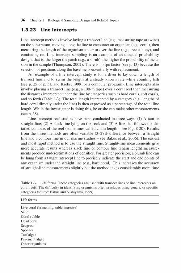
36 Chapter 1 Biological Sampling Design and Related Topics
1.3.23 Line Intercepts
Line intercept methods involve laying a transect line (e.g., measuring tape or twine) on the substratum, moving along the line to encounter an organism (e.g., coral), then measuring the length of the organism under or over the line (e.g., tree canopy), and continuing on. Line intercept sampling is an example of an unequal proabability design, that is, the larger the patch (e.g., a shrub), the higher the probability of inclu-sion in the sample (Thompson, 2002). There is no fpc factor (see p. 13) because the selection of positions along the baseline is essentially with replacement.
An example of a line intercept study is for a diver to lay down a length of transect line and to swim the length at a steady known rate while counting fi sh (see p. 25 or p. 51, and Krebs, 1999 for a computer program). Line intercepts also involve placing a transect line (e.g., a 100-m tape) over a coral reef then measuring the distances intercepted under the line by categories such as hard corals, soft corals, and so forth (Table 1-3). The total length intercepted by a category (e.g., lengths of hard coral directly under the line) is then expressed as a percentage of the total line length. While the investigator is doing this, he or she can make other measurements (see p. 38).
Line intercept reef studies have been conducted in three ways: (1) A taut or straight line; (2) A slack line lying on the reef; and (3) A line that follows the de-tailed contours of the reef (sometimes called chain length – see Fig. 8-20). Results from the three methods are often variable (3–27% difference between a straight line and a contour line in our marine studies – see Bakus et al., 2006). The easiest and most rapid method is to use the straight line. Straight-line measurements give more accurate results whereas slack line or contour line (chain length) measure-ments produce underestimations of densities. For greater precision, a plumb line can be hung from a taught intercept line to precisely indicate the start and end points of any organism under the straight line (e.g., hard coral). This increases the accuracy of straight-line measurements slightly but the method takes considerably more time
Table 1-3. Life forms. These categories are used with transect lines or line intercepts on coral reefs. The diffi culty in identifying organisms often precludes using generic or specifi c categories (source: Bakus and Nishiyama, 1999).
Life forms
Live coral (branching, table, massive)SandCoral rubbleDead coralSeagrassSpongesTurf algaePavement algaeOther organisms

1.3 Quantitative Sampling Methods 37
than simply sighting the organism below a taut line and measuring the length of tape intercepted by the organism. The ratio between the slack or contour lengths and the straight-line length increases with increasing heterogeneity, resulting in a simple mathematical decrease (i.e., error) in density estimates. Benthic marine populations are typically counted in quadrats as the organisms are observed from above, avoid-ing vertical surfaces, overhangs, and cracks and crevices in order to standardize and greatly simplify the counting. As substratum heterogeneity increases, the number of species and individuals usually increase. This is not only the result of organisms (e.g., limpets) living on vertical surfaces and overhangs, but sometimes considerable increases in species and individuals living in cracks and crevices and between coral branches (i.e., the cryptofauna) (Bakus, 1969). Thus the straight-line measurements may not refl ect either species richness or population increases related to increased physical heterogeneity. Reef heterogeneity can be estimated by comparing straight-line measurements with contour (chain length) measurements to arrive at a ratio between the two.
Line intercepts can also be used to determine if the occurrence of an organism or substratum type is closely associated with or dependent upon another organ-ism or substratum type (e.g., sponges and dead coral; sand and clams). The sequencing of organisms is recorded along transect lines and the frequencies of co-occurring organisms or substratum types are tabulated. A transition fre-quency matrix is developed (e.g., a matrix showing replacement of substratum types along a transect line) and a Chi-square equation (or G-test nowadays) is applied to the matrix to determine if any of the sequences of associated organ-isms, categories, or substratum types is signifi cant (see Chapter 3, p. 163 and Davis, 1986 for a detailed explanation of the technique). The line transect can be videotaped and analyzed in the laboratory. Surface animals and plants can be counted directly or indirectly (i.e., by assigning random points to the videotaped frames). A program for this was developed by Phillip Dustan (see PointCount99 in the Appendix).
The line intercept method works well on coral reefs because it can provide considerable information on benthic organisms and substratum types with a minimum of effort (see Marsh et al., 1984). The line intercept method (typically lines arranged perpendicular to the shore) can provide at least the following information:
1. Coral reef profi le based on depth measurements (by scuba depth gauge) at 5 or 10 m intercept lengths.
2. The rank dominance of organisms and substratum types expressed as a per-centage of the total length of the intercept line.
3. Size-frequency data on hard corals and other organisms. This is an addi-tional measurement made as one moves along a transect line. There is a bias here for large individuals, thus the advantage of using belt or strip transects rather than line intercepts, if there is suffi cient time to do so.
4. An estimation of the population densities of selected organisms.

38 Chapter 1 Biological Sampling Design and Related Topics
5. Information on whether the occurrence of an organism category (e.g., sponges, turf algae, etc.) is associated with or dependent on another category of organism or a specifi c substratum type.
6. The incidence of disease (e.g., black band disease in hard corals). This is an additional recording.
The major disadvantage of the line intercept method is that small organisms (�3 inches or �9 cm) are not often intercepted by the metric tape [measuring 1/2� or 3/4� (13 or 19 mm wide)]. For information on distance sampling see Buckland et al. (2001).
1.3.24 Strong Method
The Strong method is a line intercept method, based on the probability of inter-cepting an object along a transect line. Long ago botanists developed a complex technique using calculus with line intercepts to estimate population densities. This was later simplifi ed and improved upon by Strong (1966) whose technique is still employed today. The equation is based on the concept that the wider an organism is, the greater the probability that a transect line will intercept it. The diver selects a category or taxon of interest (e.g., sponges). When the diver intercepts a sponge under the transect line, he measures the widest width (i.e., orthogonal width) of the sponge and records it (Fig. 1-20). This procedure is continued until the 100-m line has been traversed. The data on sponge widths are then plugged into an equa-tion by Strong (1966) to give an approximation of the sponge density. The Strong method (also known as a modifi ed Eberhardt method which appeared later—see Krebs, 1999) can be applied to any organisms that can be distinguished as an individual or as a separate colony (e.g., bryozoan colony). The Strong method is an estimation of density using the harmonic mean.
Density (No. of organisms munit area
total transect len2 ) �
1
M ggth∑
where:
Σ � sum
M � maximum orthogonal width (m) of an organism intercepting the transect line
unit area (�1 m2 for example)
total transect length � 100 m (in this example).
Example
Corals (table Acropora) or trees intercepting a transect line (measuring the greatest width of the tree canopy)
Intercepted widths (m) are: 2, 3, 1, 4, 3, 1, 3, 2

1.3 Quantitative Sampling Methods 39
Density
or
�1
2
1
3
1
1
1
4
1
3
1
1
1
3
1
2
0 50 0 333 1 0 0 25 0 333 1 0 0 333 0 5. . . . . . . . 00
4 2491
1000 04249Density organisms m2� �. .
1.3.25 Weinberg Method
The Weinberg (1981) method is a line intercept method, based on the probability of an object intercepting the line. It has been buried in the coral reef literature for many years, largely unavailable to terrestrial and freshwater biologists. In the Weinberg method (1981), lengths of organisms intercepted by a transect line are recorded. This method works well with circular organisms (e.g., some hard corals, shrubs) that are larger than about 1.0 m in diameter (Fig. 1-21).
The equation is as follows:
Density
No. of interceptstransect length
mean organism inte�
rrcept length coral colony size correction factor� 1 156. ( )
Figure 1-20. Strong method. Measuring the greatest orthogonal width along a transect or line intercept. For smaller plants – measurements are made below the line (e.g., with grasses, forbs, and small shrubs) and above the line (e.g., with larger plants). For trees, the canopy width is measured.

40 Chapter 1 Biological Sampling Design and Related Topics
Example
Corals intercepting a 50 m transect line
Organism intercept length (m) –2.0, 3.4, 1.2, 3.2, 4.5
D � �5 50
2 86 1 1560 0303
. ( . ). coral m2
A computer program (Weinberg) for this is found in the Appendix. See Weinberg (1981) and Nishiyama (1999).
Gregory Nishiyama Correction for the Weinberg Equation:
In the Weinberg equation for the estimation of the density of an organism, he approximates the organism’s diameter from the intercept lengths of the organism on the transect line. Thus, he multiplies the average intercept length by the correction factor 1.156. Weinberg assumed that the average intercept length that is found mid-way between the maximum and minimum possible intercept lengths to be the aver-age intercept length (Fig. 1-22). However, Weinberg’s midpoint does not designate the average chord or intercept length. To obtain this, one must add up sample lengths (from maximum to minimum possible lengths) and fi nd the average (Fig. 1-23).
Figure 1-21. Weinberg method. Measuring the length of an organism intercepted by a line. For terrestrial studies this includes plants below (e.g., shrubs or grasses) and above (trees) the line. For trees the length of the canopy above the line is measured.

1.3 Quantitative Sampling Methods 41
The fi nal correction factor comes out to be 1.301. So the Weinberg equation becomes:
No. of intercepts / transect length
mean intercept length�1 3. 001
Although this correction factor may not seem very different from Weinberg’s 1.156, there is a 13% difference in these two numbers that translate to a 13% dif-ference in their density estimates. This is a signifi cant difference when ideally an estimation method should have a maximum of a 10% error. This new correction fac-tor was tested by Nishiyama on 30 simulations and shown to produce more accurate estimates than the original Weinberg correction factor. This new correction factor needs to be tested in the fi eld.
Figure 1-22. Weinberg’s intercept length and the true intercept length. See text for explanation.
True averageintercept length
Weinberg’s interceptlength Weinberg’s midpoint
(Not to scale)
Figure 1-23. Average of intercept lengths. See text for explanation.
Average of interceptlengths

42 Chapter 1 Biological Sampling Design and Related Topics
1.3.26 Nishiyama Method
The Nishiyama method is a line intercept method. Nishiyama has developed a den-sity estimate technique which takes into consideration the orientation of organ-isms relative to the transect line. This method was used to estimate the densities of strongly ovate intertidal organisms (e.g., mussels). The transect lines are parallel to the shoreline.
Gregory Nishiyama Density Orientation Method:
Although such methods as Weinberg and Strong can estimate the densities of organisms, they do not take into consideration the effect of the orientation of the organisms. If the orientation of the organism is random, such methods above may work successfully. However, if there is a bias in the orientation of the organism (around 20% or more bias in a particular direction – e.g., organisms oriented more or less parallel to the incoming waves) and it is ovate in shape (especially if the organism’s length to width ratio � �3) (e.g., mussels, some chitons) the error in the estimation of density can be considerable. The following equation is an exten-sion of the Weinberg equation, which addresses the problems with orientation and shape.
To use the proposed equation, the investigator must place each organism inter-cepting the transect line into one of four categories based on its orientation relative to the line. Although each category is assigned an angle designation, the categories actually represent ranges of angles. When an organism has a particular orientation at or close to a particular category, it is placed into that category. For example, if an organism has an orientation of 37 degrees relative to the line, it is placed into the 30-degree category. Alternatively the user can divide the circle into numerous categories with angle ranges, however, this may make the collection of data more diffi cult. Instead, if it is close to one of four categories, the user should simply put it in its proper angle group. Once these data are gathered, each angle category is analyzed separately and then all the density estimates are summed. This will give the total density.
Each organism intercepting the transect line is placed in one of the orientation categories (Fig. 1-24).
Figure 1-24. The four positions of mussels relative to a tape measure or intercept line, used in the Nishiyama technique for determining densities of intertidal organisms. See text for explanation.
1
(90°) (60°) (30°) (0°)
2 3 4
or or

1.3 Quantitative Sampling Methods 43
These counts and the organism’s dimensions are then placed into the appropriate sections of the following equation:
90 60 30 0� � � �
� �
( ) ( ) ( ) ( )
Density ( number of individuals m TL2 )
n
L
nn
L
n
L
n
WTL TL TL
( . ) ( . )0 87 0 50� �
where
n � number of intercepts (for each orientation category—see Figure 1-24)
TL � transect length (e.g., in meters)
L � mean organism length (e.g., in meters)
W � mean organism width (e.g., in meters)
Note: All measurements must be in the same units
Example
Assume that the numbers of mussels in different orientations � 10, 5, 20, 10; transect length � 100 m; average mussel lengths � 5, 6, and 7 cm; and average mussel width � 3 cm.
D
D
� � � �
�
101000 05
5100
0 87 0 06
20100
0 5 0 07
101000 03
2
. ( . )( . ) ( . )( . ) .
�� � �
�
1 6 3
12 2D mussels m
In a dozen simulations where there was a bias in the organism’s orientation, up to a 33% error between the density estimates of the Weinberg method and Nishiyama method was observed. That is, the Nishiyama method was more accurate than the Weinberg method due to the consideration of the orientation of the organisms. A computer program (Nishiyama) for this is presented in the Appendix. The Nishi-yama method needs to be tested in the fi eld.
Some of these plotless methods and others have defi ciencies that produce crude estimates and one should consult references or specialists before using them. How-ever, sometimes they are the only practical sampling technique available and there-fore of use. When various plot and plotless estimates are compared with a com-plete census (i.e., total count), there are often considerable differences in the results (even using stratifi ed random sampling), an important point to remember. This is especially true when relatively few samples are taken or organisms are highly aggregated, which often produce inaccurate estimates. See Venrick (1971), Weisberg and Bowen (1977), and Yates (1981).
A summary of 12 terrestrial and marine density estimate studies indicated that the Strong method was most accurate among several methods tested for station-ary organisms (Bakus et al., 2006). Moreover, it is best used for those organisms

44 Chapter 1 Biological Sampling Design and Related Topics
measuring more than about 0.3 m (1 ft) in diameter (e.g., corals, shrubs, trees). Strati-fi ed random sampling ranked second best and the Third Nearest Object the third best (Bakus et al., 2006). Goedickemeier et al. (1997) found that at a scale of 10–50 km2, stratifi ed random sampling creates an accurate picture of small-scale vegetation pat-tern at low sampling effort.
Additional distance sampling methods include point counts, point transect sam-pling, trapping webs, and cue counting, among others (Buckland et al., 2001).
1.3.27 Mark (or Tag) and Recapture (Mark and Resight) Techniques
Mark-recapture techniques consist of marking or tagging a mobile species one day (Table 1-4), then returning to recapture the species and count the individuals the next or succeeding days. An estimate of the population in the area is thus ac-quired. Capture–recapture methods are now frequently used for the estimation of birth, death (or survival), and emigration rates (Southwood and Henderson, 2000). Mark-recapture methods have several advantages over line transect sampling for wildlife (see Buckland et al., 2001, for details). However, mark-recapture fi eld costs are substantially higher to achieve the same precision on abundance estimates than line transect sampling (Borchers et al., 2002). For example, mark- and-resight techniques for fi shes take 13–15 times more diver time than a visual belt transect estimation (Davis and Anderson, 1989). Although mark-and-resight techniques
Table 1-4. Methods of marking and tagging organisms.
Molluscs: Quick-drying paint; notches with fi le, carborundum wheel or dentist’s drill; adhesive tape; metal; Peterson discs; Plastic tags
Crustaceans: Spaghetti and dart tags; punching telson, etc. (problem with molting); dyes for shrimp (Penaeus).
Echinoderms: Monofi lament nylon (sea urchins)Fishes: Branding (sharks); clipping fi ns; internal magnetic or radioactive tags; external tags,
dart tag best, plastic, inserted just below dorsal fi nTurtles: Magnetic tag injected into muscleBirds: Aluminum, colored celluloid or plexiglass bands; sonic markerMammals:
a. Seals and sea lions — hot iron branding best, good for over 20 years on fur seals; metal tags in forefl ipper good for 8 years.
b. Cetaceans — stainless steel tube coated with penicillin, shot into whales, recovered in boilers, reward offered.
Newest Methods: Fluorescent paints, injection, tattoos, clipping of wings or fi ns, rare elements, radioactive isotopes, radioactive labels and incorporation in tissues, transponders and sonic tags, radio-telemetry (radio collars) and micro-videocameras (e.g., attached to elephant seals or great white sharks). For further information see Seber (1982), Sutherland (1996), and especially Southwood and Henderson (2000).

1.3 Quantitative Sampling Methods 45
produce more accurate estimations of fi sh populations than visual belt transects, the method is prohibitively expensive for regular use (Hallacher, 2004). Mark-recapture abundance estimates are more sensitive to failure of assumptions than line transect estimates.
Population marking techniques are often classifi ed as batch (group) or individ-ual tagging techniques (Southwood and Henderson, 2000). Thomson (1962) used 12 different tags and markers on 183,113 shellfi sh, crustaceans, fi shes, and whales. The overall recovery was 5.5%, comparable to other previous large studies on tagging and marking. Because the average recovery rate for many tagged or marked marine organisms is about 5%, hundreds or thousands of animals may need to be marked or tagged to provide meaningful results (Thomson, 1962). For this reason, a sample size estimation needs to be made before starting the marking or tagging program (Krebs, 1999). Dale Kiefer (pers. comm.) reports that tagging recovery for southern sea elephants (Mirounga leonina) is as high as 90%. Mark-recapture techniques are only appropriate for use with mobile animals such as shrimp and fi shes, but only with fi shes that remain in the study area over several days or more.
Some of the recent developments in tagging involve the use of satellite and data storage tags. Seabirds such as the Wandering Albatross (Diomedia exulans) are followed with satellite tags (PPT or Platform Terminal Transmitter). Data Storage Tags (DST-CTD) are used for tagging large fi shes such as tuna. They measure conductivity (salinity), temperature, and depth. The system consists of a tag, communication box, computer, and software. Pop-up satellite archival tags (PSAT) measure ambient light (for latitude and longitude), temperature, and depth and transmit this information from the sea surface to an Argos satellite system. The tags can be programmed to detach at a preset depth or preset time. Among animals studied in this manner are Bluefi n Tuna (Thunnus thynnus), Blue Marlin (Makaira nigricans), Tiger Shark (Galeocerdo cuvier), Blue Shark (Prionace glauca), Great White Shark (Carcharodon carcharias), Black-footed Albatross (Phoebastria nigripes), and the Southern Sea Elephant (Mirounga leonina). A fi sh algorithm developed by Frank O’Brien was incorporated into the computer program Easy (developed by Dale Kiefer, Department of Biological Sciences, University of Southern California) to analyze data collected by satellite tags. This analysis technique can also be applied to seabirds (e.g., Laysan Albatross — Phoebastria immutabilis) and marine mammals (e.g., sea lions, elephant seals, whales). One of the latest developments in fi sh management is the use of Mini GPS fi sh tags (Gudbjornsson et al., 2004).
Mark-recapture methods used in the past were based on a number of as-sumptions (Bakus, 1990): (1) The animal will not be affected by the marking or tag-ging (see Murray and Fuller, 2000); (2) The marks are not lost; (3) The population is sampled randomly and the age groups and sexes are equally available, that is, each individual has an equal probability of capture; (4) The sampling time is small rela-tive to the total time of the study; (5) The population is either closed or immigration and emigration can be measured; (6) No births or deaths occur between sampling periods or some correction for this must be made; and (7) The initial capture does not effect subsequent recapture. It should be emphasized that a number of these

46 Chapter 1 Biological Sampling Design and Related Topics
assumptions (e.g., random sampling and age groups and sexes are equally available) are no longer present in recent models.
The simplest mark-recapture method is the Simple Lincoln Index (for closed populations). A closed population is one in which there are no gains by births or immigration and no losses by deaths or emigration. This is based on the Petersen method (Krebs, 1999); also see a modifi ed Petersen method (Arnason, 1973). The animals are marked then recaptured on a subsequent day, and marked and unmarked animals are counted. The second count assumes random sampling. This index is seldom used today except perhaps for some student fi eld exercises.
1.3.27.1 Lincoln Index
Example:
Fishes (e.g., territorial damselfi sh) are collected from the ends and the middle of a large tidepool during low tide. The fi shes (64) are tagged then released into the same tidepool. The next day damselfi shes are recollected from the ends and middle of the same tidepool. Count the tagged (6) and untagged (56) animals. Use the Simple Lincoln Index to calculate the approximate population size (see below). Note that the answer is not a true density estimate but an estimated total population size, applicable to mobile animals only (see Green, 1979, and Krebs, 1999, for further information). Moreover, the assumption that immigration and emigration has not occurred is likely to be invalid for many species of fi shes. Other assumptions are also violated.
Pa n
r�
( )( )
( )
where
P � total number of individuals (estimated population size)
a � number of animals marked in fi rst sample
n � total number of individuals captured in second sample
r � number of marked individuals captured in second sample
P P��
�( )( )
( )
64 56 6
6661 tidepool damselfish
The 95% confi dence limits for a Poisson frequency distribution are 286 tidepool damselfi sh and 1097 tidepool damselfi sh (see Krebs, 1999, for a detailed discussion). This is as low or as high as we would expect the damselfi sh population to be with 95% confi dence (i.e., one in 20 chance of being below 286 or above 1097).
1.3.27.2 Sampling at three or more times (for open
populations)
Open populations are those in which individuals of a species are subject to gains by birth or immigration and losses by death or emigration. Three methods

1.3 Quantitative Sampling Methods 47
have been commonly used for this type of sampling, the Seber method, the Schna-bel method, and the Manly–Parr method. The Jolly–Seber or Cormack–Jolly–Seber models were often preferred because they account for recruitment and mortality and are fully stochastic (Southwood and Henderson, 2000). The calculations are quite lengthy. The classical Jolly–Seber method for open populations is now pre-sented (Sutherland, 1996). It requires that at least three samples should be taken and animals should be individually marked or have marks that are batch-specifi c (Tables 1-5 and 1-6).
There are many new mark-recapture techniques for both closed and open populations. Among them are modifi ed Jolly–Seber models such as the Pradel model, Pollock model, Band Recovery model, Joint Live and Dead Encounter model, Known Fate model, Encounter Histories model, and Bayesian models, among others. There are also many computer programs available for these mod-els. One in current favor by many investigators is the program MARK that can handle some 16 variables. The MARK program can be downloaded from the Internet for free:
http://www.cnr.colostate.edu/∼gwhite/mark
See also: http://www.phidot.org/software/
Sutherland (1996) discusses several mark-recapture methods with examples. Southwood and Henderson (2000) list computer software for capture-recapture methods and discuss Moran–Ricker curves. Statistical tests used to detect variation in catchability (e.g., Cormack’s test) are presented by Southwood and Henderson (2000). A recent handbook on capture-recapture analysis is presented by Amstrup et al. (2006); see also Begon (1979).
Table 1-5. Recording the composition of each collection sample for the Jolly–Seber method when marks or tags are batch-specifi c (source: Sutherland, 1996).
Days on which previously captured Number of animals
1 2 30b 0b 0b 40�a 0b 0b 100b �a 0b 90b 0b �a 11�a �a 0b 2�a 0b �a 20b �a �a 1�a �a �a 0b
aPlus signs indicate that an animal was caught on that day.bzeros that it was not. This example refers to sample number 4 in a hypothetical study.

48 Chapter 1 Biological Sampling Design and Related Topics
Table 1-6. An example of the Jolly–Seber method of mark or tag and recapture analysis (source: Sutherland, 1996).
The Jolly–Seber method
Defi nitionsni � total number of animals caught in the ith sampleRi � number of animals that are released after the ith samplemi � number of animals in ith sample that carry marks from previous captures
mhi � number of animals in the ith sample that were most recently caught in the hth sample
ExampleBlack-kneed Capsides Blepharidopterus angulatus caught at 3- or 4-day intervals in a British apple orchard (Jolly 1965).The data are best summarized in a table of mhi values, with ni and Ri values across the top and the mi values (which are the sums of the mhi values in the column above) across the bottom. Thus in the table below, 169 insects were caught in sample 3 (n3) of which 164 (R3) were released; 3 of them bore marks from sample 1 (but not from sample 2) (m13) and 34 bore marks from sample 2 (m23), giving a total of 37 marked insects (m3).
i 1 2 3 4 5 6 7 8 9 10 11 12 13ni 54 146 169 209 220 209 250 176 172 127 123 120 142Ri 54 143 164 202 214 207 243 175 169 126 120 120 —
h rh zi
1 10 3 5 2 2 1 0 0 0 1 0 0 24 —2 34 18 8 4 6 4 2 0 2 1 1 80 143 33 13 8 5 0 4 1 3 3 0 70 574 30 20 10 3 2 2 1 1 2 71 715 43 34 14 11 3 0 1 3 109 896 56 19 12 5 4 2 3 101 1217 46 28 17 8 7 2 108 1108 51 22 12 4 10 99 1329 34 16 11 9 70 121
10 30 16 12 58 10711 26 18 44 8812 35 35 60
mi 0 10 37 56 53 77 112 86 110 84 77 72 95
The table contains two other sets of summations:rh � the number of animals that were released from the hth sample and were
subsequently recaptured; these are simply the row sumszi � the number of animals caught both before and after the ith sample but not in the
ith sample itself; zi is the sum of all the mhi that fall in columns to the right of column i and all rows above row i; thus the dashed lines in the table delimit the mhi values that must be summed to obtain z4, for example
Parameter estimatesM̂
i � number of marked animals in the population when the ith sample is taken (but not including animals newly marked in the ith sample).
� mi � (Ri � 1)zi(ri � 1)

1.3 Quantitative Sampling Methods 49
(continued)
Table 1-6. (continued)
N̂i � population size at the time of the ith sample� M̂i (ni � 1)/(mi � 1)
Φi � proportion of the population surviving (and remaining in the study area) from the ith sampling occasion to the (i � 1)th
� M̂i � 1/(M̂i � mi � Ri)B̂i � number of animals that enter the population between the ith and (i � 1)th
samples and which survive until the (i � 1)th sampling occasion.� N̂i � 1 � Φi (N̂i � ni � Ri)
Note that one cannot calculate M̂ for the last sample. N̂ for the fi rst or last, Φ for the last two, or B̂ for the fi rst or last two. M̂1 is bound to be zero.Calculations are eased if laid out systematically:
ˆ ( ) ( ) .ˆ ( ) ( ) .ˆ
M
M
2
3
10 143 1 14 80 1 34 89
37 164 1 57 70 1 169 46
� � � � �
� � � � �
MM4 56 202 1 71 71 1 256 18� � � � �( ) ( ) .
etc.
ˆ . ( ) ( ) .ˆ . ( ) ( )
N
N
2
3
34 89 146 1 10 1 466 12 466
169 46 169 1 37 1 7
� � � � �
� � � � 558 11 758
256 18 209 1 56 1 943 82 9444
.ˆ . ( ) ( ) .
�
� � � � �N
etc.
ΦΦΦ
1
2
3
34 89 0 0 54 0 646
169 46 34 88 10 143 1 009
25
� � � �
� � � �
�
. /( ) .
. /( . ) .
66 18 169 46 37 164 0 864. /( . ) .� � �
etc.
ˆ . . ( . ) .ˆ . . (
B
B
2
3
758 11 1 009 466 26 146 143 290 68
943 82 0 864 75
� � � � �
� � 88 11 169 164 293 13. ) .� � �
etc.Confi dence limits for N̂i
Methods usually presented for calculating confi dence limits of Jolly–Seber estimates are inadequate for the commonly encountered sample sizes. The following method, due to Manly, provides better limits.Calculate a transformation of each N̂i and the standard error of the transformation.
T N n N
sM m R
M
i e i i i
Ti i i
ii
� � �
�� � �
�
log . log .0 5 0 5 3 8
1
1
e
1
1
1
11
1
1
1r R m ni i i i��
��
��
�
For example, the transformation for N̂2 is
T
sT
2 466 26 0 5 0 5 3 146 8 466 26 5 6643
34 892
� � � �
�
log . . log [ . ( ) ( . )] .
.
e e
�� � �
� ��
��
��
��
10 143 1
34 89 1
1
80 1
1
143 1
1
10 1
1
146 10 3
..
3309
ˆ
ˆ
ˆ
ˆ

50 Chapter 1 Biological Sampling Design and Related Topics
Table 1-6. (continued)
Calculate confi dence limits for Ti, and their exponents:
T T s W i
T T s W ii i T i
T
i i T iT
i
i
L L
U U
e L
e U
� � �
� � �
1 65
2 45
. :
. :
Continuing the same example:
T W
T2L 2L
U
e� � � � �
� �
5 664 1 65 0 331 5 118 166 98
5 664 2 4
5 118
2
. . ( . ) . ; .
. .
.
55 0 331 6 475 648 696 475( . ) . ; ..� � �W2U e
95% confi dence limits are given by
( ) ( )4 16 4 162 2W n W W n Wi i i i i iL L U Uand� �
For the example of N̂2 the limits are
[ ( . ) ] ( . )4 166 98 146 16 166 98 2482� �
and
[ ( . ) ] ( . )4 648 69 146 16 648 69 7242� �
Goodness-of-fi t testThe test is applied to each sample in turn, except the fi rst and the last. All animals caught in the sample are categorized as follows:
f1 � fi rst captured before this sample, subsequently recapturedf2 � fi rst captured before this sample, not subsequently recapturedf3 � fi rst captured in this sample, subsequently recapturedf4 � fi rst captured in this sample, not subsequently recaptured
Calculate
a f f a f f a f f a f f
n f f f f
g f f
1 1 2 2 3 4 3 1 3 4 2 4
1 2 3 4
1
� � � � � � � �
� � � �
�
, , ,
log ,e gg a a
G g g n n
e
e
2
1 22
�
� � �
log
( log )
∑∑
Meadow Voles Microtus pennsylvanicus trapped over 6 occasions in Maryland, USA, by J. D. Nichols (Pollock et al. 1990) provide an example for this calculation.For the second sample the fi gures were
f f f f
a a a a
n
g
1 2 3 4
1 2 3 4
1
47 31 29 14
78 43 76 45
121
47
� � � �
� � � �
�
�
, , ,
, , ,
logg log log log .
log loge e e e
e e
47 31 31 29 29 14 14 422 01
78 78 43 42
� � � �
� �g 33 76 76 45 45 1001 99
121 121 580 29
2 42
� � �
� �
�
log log .
log log .
(
e e
e en n
G 22 01 1001 99 580 29 0 62. . . ) .� � �
This G should be compared with χ2 with 1 degree of freedom.The G values for samples 2, 3, 4 and 5 of Nichols’s study of voles, with their associated probabilities, are
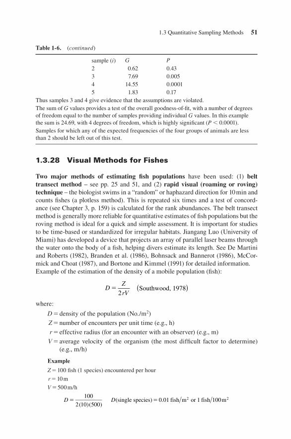
1.3.28 Visual Methods for Fishes
Two major methods of estimating fi sh populations have been used: (1) belt transect method – see pp. 25 and 51, and (2) rapid visual (roaming or roving) technique – the biologist swims in a “random” or haphazard direction for 10 min and counts fi shes (a plotless method). This is repeated six times and a test of concord-ance (see Chapter 3, p. 159) is calculated for the rank abundances. The belt transect method is generally more reliable for quantitative estimates of fi sh populations but the roving method is ideal for a quick and simple assessment. It is important for studies to be time-based or standardized for irregular habitats. Jiangang Luo (University of Miami) has developed a device that projects an array of parallel laser beams through the water onto the body of a fi sh, helping divers estimate its length. See De Martini and Roberts (1982), Branden et al. (1986), Bohnsack and Bannerot (1986), McCor-mick and Choat (1987), and Bortone and Kimmel (1991) for detailed information.Example of the estimation of the density of a mobile population (fi sh):
DZ
rV�
2Southwood, 1978( )
where:
D � density of the population (No./m2)
Z � number of encounters per unit time (e.g., h)
r � effective radius (for an encounter with an observer) (e.g., m)
V � average velocity of the organism (the most diffi cult factor to determine) (e.g., m/h)
Example
Z � 100 fi sh (1 species) encountered per hour
r � 10 m
V � 500 m/h
D D� �100
2 10 5000 01 1 100 2
( )( )( ) .single species fish m or fish m2
Table 1-6. (continued)
sample (i) G P2 0.62 0.433 7.69 0.0054 14.55 0.00015 1.83 0.17
Thus samples 3 and 4 give evidence that the assumptions are violated.The sum of G values provides a test of the overall goodness-of-fi t, with a number of degrees of freedom equal to the number of samples providing individual G values. In this example the sum is 24.69, with 4 degrees of freedom, which is highly signifi cant (P � 0.0001).Samples for which any of the expected frequencies of the four groups of animals are less than 2 should be left out of this test.
1.3 Quantitative Sampling Methods 51

52 Chapter 1 Biological Sampling Design and Related Topics
1.3.29 Narcotizing Agents and Poison Stations
Fishes can be collected alive by using a narcotizing agent such as quinaldene. How-ever, some people are sensitive to the chemical. The quinaldene is fanned among branches of coral or openings in rocks. It works successfully only if there is no cur-rent to disperse the chemical.
Fish populations have been estimated by setting up poison stations. This can be done efficiently using perhaps a dozen divers. Plastic gallon (3.8 l) bags are filled with rotenone or rotenone derivative (Noxfish, Chemfish) and a sol-vent (e.g., alcohol). Each diver carries a plastic bag with chemicals down to the reef. The divers then break the bag in unison and distribute the rotenone by fanning the water over the coral with their swim fins. Fishes affected by the rotenone begin to swim out of the corals around 15 minutes after the applica-tion of rotenone. Typically the last fishes to exit the corals are moray eels, after about 45 min. The diver uses a dip net and goody bag to capture and secure the fishes. The fishes must be captured quickly as they often reenter the reef and probably die. Predators on coral reefs (e.g., large jacks, sharks) may take many of the squirming fishes before the diver has an opportunity to catch them. Thus the resulting fish catch is an underestimation of the population of fishes in the area.
1.4 OTHER METHODS OF ESTIMATING THE ABUNDANCE OF POPULATIONS
1.4.1 Comparison of Estimated Populations with Other Methods
(a) Measure a population by random sampling and compare the results with a relative method (e.g., trap organisms by random sampling and compare them with the number of animals observed per hour).
(b) Calculate the regression of some index with an actual population (e.g., the density of a species of kelp by random sampling and by actual count along a line with depth).
1.4.2 Removal Trapping or Collecting
A known number of animals are removed from a habitat by trapping, and the rate at which the trap catches decrease indicates the size of the total population. Eber-hardt’s Removal Method is discussed by Krebs (1999). As mentioned previously, removal methods have poor precision and a large potential for bias (Buckland et al., 2001).

1.4.3 Other Methods
1.4.3.1 Indirect Distance Sampling
The population of elephants in dense forests in Kenya is estimated by counting fresh fecal droppings. These elephants are wary of people and are seldom seen in some biological preserves (e.g., preserve near Malindi). The fresh nests of birds can also be tallied. Point transect sampling can be used for counting birds and whales (Buckland et al., 2001). Typically the lines and points are selected ran-domly. The area surrounding the point is surveyed over a standardized time pe-riod for birds, for example, and the distance from the point to the site where the bird was spotted is measured. Laser binoculars can be used for precise measure-ments. Spot mapping involves intensive mapping of territories and home ranges of target species (typically birds) at randomly chosen points within the study area (Hallacher, 2004).
1.4.3.2 Rare Species
Thompson (2004) and colleagues discuss the sampling of rare, sparse, or elusive species. Rare species can be defi ned as species with a low probability of detec-tion. Sparse species are those that occur in small clumps but over large areas. Elusive species are species with secretive or nocturnal behavior. Among the many techniques discussed in Thompson (2004) are aerial surveys, distance sampling, intercept sampling, mark-recapture, adaptive sampling, two-phase or stage or dou-ble adaptive sampling, adaptive cluster sampling, sequential sampling, point count method of sampling for birds, sighting probability models, patch-occupancy models, occupancy estimation using likelihood methods, resource selection functions for the design of unequal probability sampling, Bayesian estimation, spatial modeling of plants, noninvasive genetic sampling (e.g., mitochondrial DNA or nuclear DNA in hair and feces), photographic sampling of elusive mammals in tropical forests, and banding and PIT tagging in bats.
1.4.3.3 Coral Reef Surveys
Live cover of hard corals has typically been measured in two ways: (1) by eye, and (2) by line transect. Live cover by eye involves: being towed by a rope or Manta board behind a boat (Figure 8-22), or using an underwater scooter (e.g., Farallon scooter – see Fig. 1-25). Towing a person with a boat works well but speed must be reduced be-cause it is diffi cult to hold on to the rope. A Manta board is preferable. Sometimes the diver may be followed by sharks. The underwater scooter is a wonderful method of surveying reefs although velocities must be reduced until the diver develops suf-fi cient holding strength. There are two dangers in using underwater scooters. The scooters travel so fast that it is easy to reconnoiter down to 60 m or deeper and be unaware of the depth. The battery may die thus it is important to travel in pairs for safety reasons. Although slow, one scooter can tow two people through the water
1.4 Other Methods of Estimating the Abundance of Populations 53

54 Chapter 1 Biological Sampling Design and Related Topics
back to the ship. In any case, the observer must be competent in coral identifi cation. See p. 24 for information on line transects.
A relatively recent large study of coral reefs in the western Atlantic included the following techniques (Lang, 2003): Benthic organisms – (1) line intercepts (10 m long), (2) measuring hard coral dimensions, (3) recording diseases (e.g., black band), (4) using small quadrats for estimating the percentage of algal cover, and (5) belt transect counts of the sea urchin Diadema. Fishes – (1) belt transects (30 m long), (2) a roaming or roving population estimation, (3) counting fi sh in 7.5 m diameter cir-cles, and (4) fi sh bites in m2 plots (total of fi ve plots). See this chapter and Chapter 3 for discussions of these topics.
1.4.3.4 Artifi cial Reefs
Artifi cial reefs enhance substrate or habitat heterogeneity and lead to an overall in-crease in diversity over time (Bortone and Kimmel, 1991). The primary reason for establishing artifi cial reefs is to increase lobster and fi sh populations and to enhance sport diving, especially on sunken ships. Artifi cial reefs attract and con-centrate commercially viable fi sh populations at a new site, and then overfi shing oc-curs. The newest approach is to develop artifi cial reefs to enhance the populations of specifi c species of fi sh (e.g., see http://myfwc.com/marine/ar/index.asp). Examples of artifi cial reefs are shown in Fig. 1-26. Recent innovations include limestone reef restoration using electrodes (cathodic reef stimulation) to induce mineral accretion [CaCO3 and Mg (OH)3] on artifi cial reef frames. This produces coral reef growth (see http://www.globalcoral.org/third_generation_artifi cial_reef.htm).
Artifi cial reef colonization is often very rapid and shows similar and repeat-able patterns in temperate waters. When abiotic conditions are stable, biological fac-tors such as competition and predation are usually important for limiting population sizes and controlling assemblage (community) composition.
Bortone and Kimmel (1991) present a list of variables commonly measured on ar-tifi cial reefs and references to methods of assessing and monitoring artifi cial habitats. Techniques include collecting data on individual organisms (e.g., body size, feeding habits, territory size), on populations (e.g., natality, mortality, age classes), nonvisual methods for fi sh and invertebrates (e.g., hook and line, nets, hydroacoutistics), and
Figure 1-25. Farallon underwater scooter. An excellent device for the underwater reconnaissance of reefs. Some underwater scooters cost less than $100 but are limited to a depth of 65 ft (20 m). See text for explanation. Source: http://www.faralonusa.com/product.html

visual methods (diver transects, species-time counts, predation, still photos, videos, ROVs, and manned submersibles). For further information see Seaman and Sprague (1991), Seaman (2000), and especially the Internet. See Berger (1993 or later) for a bibliography on artifi cial reefs.
Recent reefs in North America available for divers and fi sherfolk include: (1) Comanche reef, Charleston, South Carolina [50 subway cars at a depth of up to 29 m (95 ft)]; (2) Tenneco Towers, Fort Lauderdale, Florida [oil and gas exploration
Figure 1-26. Examples of artifi cial reefs. Source: Bortone and Kimmel (1991).
Payao (bamboo raft) Kannizzati (cork raft) Sphere
Mid–water FAD Ballasted trees Plastic seaweed
Stones or quarry rock Concrete cubes Concrete culvert
Ballasted tires Plastic pipe/concrete block(experimental)
Derelict vessel
Steel reef(low profile)
Steel reef(high profile)
Petroleum platform(obsolete)
1.4 Other Methods of Estimating the Abundance of Populations 55

56 Chapter 1 Biological Sampling Design and Related Topics
platforms at a depth of up to 40 m (130 ft)]; (3) USS Spiegel Grove, Key Largo, Florida [156 m (510 ft)] Navy landing ship at a depth of up to 40 m (130 ft); (3) Snake Island Wrecks (two ships), Vancouver Island, British Colombia, at a depth of up to 40 m (130 ft); and (4) HMCS Yukon, 112 m (366 ft) Canadian destroyer escort ship, San Diego, California, at a depth of up to 31m (101 ft). The U.S. Navy recently sank one of its air-craft carriers (USS Oriskany) off the coast of Pensacola, Florida (Gulf of Mexico).
1.4.3.5 Further Methods of Small Scale Sampling
Populations may also be estimated by animal products (e.g., worm tubes, barnacle shells, exoskeleton remains, bird nests, feces) or by effects (e.g., introduction of a known number of animals into a specifi ed habitat or exclusion of grazers from a habitat, amount of plant consumed). Seabird colony populations can be estimated by fl ushing the birds and whales by cue counting (e.g., whale blows per unit area per unit time). See Borchers et al. (2002) and Gore et al. (2000) for further information. Krebs (1999) discusses methods of estimating abundances of populations with radio transmitters, and a series of enumeration methods used with small mammals. South-wood and Henderson (2000) discuss observation of birds by radar, hydroacoustic methods, automatic fi sh counters (e.g., for salmon moving upstream), oral detec-tion, trapping including aquatic light traps, baits and lures including kairomones and pheromones, sound, and so forth. Change in ratio methods has poor precision (Borchers et al., 2002). See also Buckland et al. (2001). Other methods of sampling include link-tracing designs (e.g., network sampling), multistage designs, variable circular plots or point transects, and spatial sampling or kriging (Thompson, 2002). Resource or habitat selection sampling is discussed by Manly et al. (2002).
1.4.4 Large Scale Sampling
Techniques that sample large-scale areas include: (1) aerial surveys including pho-tography; (2) satellite imagery; and (3) hyperspectral imaging. Aerial surveys include counts or population estimates of marine birds (e.g., auks, Family Alcidae) and ma-rine mammals (e.g., whales, walruses (Odobenus rosmarus) – see Kauwling and Bakus, 1979). Photography from aircraft has been used for many years. Among the methods are infrared photos of forests or of kelp beds along the coast. Other types of aerial photography include photos from cameras mounted on kites and pigeons, un-manned aerial vehicles (UAVs), and balloon airships. Aircrafts (airplanes) generally operate between 600 ft (183 m) and 100,000 ft (30,488 m). Radar offers the greatest potential for foul weather remote sensing, but is relatively expensive.
The main types of instrumentation used in large-scale sampling include the spec-trometer (optical), radiometer (thermal), and radar or microwave scanning (weather). Multispectral scanning began in the 1970s with the digital remote sensing Land-sat satellite. Two primary instruments are used in multispectral scanning: (1) MSS (multispectral scanner system) provides from orbit visible and infrared images as high as an 80-m resolution in four bandwidths. MSS systems extend the light recep-tion range into the infrared with much higher spatial resolution than photographic
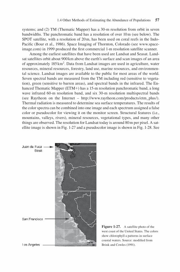
systems; and (2) TM (Thematic Mapper) has a 30-m resolution from orbit in seven bandwidths. The panchromatic band has a resolution of over 10 m (see below). The SPOT satellite, with a resolution of 20 m, has been used on coral reefs in the Indo-Pacifi c (Bour et al., 1986). Space Imaging of Thornton, Colorado (see www.space-image.com) in 1999 produced the fi rst commercial 1-m resolution satellite scanner.
Among the earliest satellites that have been used are Landsat and Seasat. Land-sat satellites orbit about 900 km above the earth’s surface and scan images of an area of approximately 185 km2. Data from Landsat images are used in agriculture, water resources, mineral resources, forestry, land use, marine resources, and environmen-tal science. Landsat images are available to the public for most areas of the world. Seven spectral bands are measured from the TM including red (sensitive to vegeta-tion), green (sensitive to barren areas), and spectral bands in the infrared. The En-hanced Thematic Mapper (ETM�) has a 15-m resolution panchromatic band, a long wave infrared 60-m resolution band, and six 30-m resolution multispectral bands (see Raytheon on the Internet – http://www.raytheon.com/products/etm_plus/). Thermal radiation is measured to determine sea surface temperatures. The results of the color spectra can be combined into one image and each spectrum assigned a false color or pseudocolor for viewing it on the monitor screen. Structural features (i.e., mountains, valleys, rivers), mineral resources, vegetational types, and many other things are observed. The resolution for Landsat today is around 80 m per pixel. A sat-ellite image is shown in Fig. 1-27 and a pseudocolor image is shown in Fig. 1-28. See
1.4 Other Methods of Estimating the Abundance of Populations 57
Figure 1-27. A satellite photo of the west coast of the United States. The colors show chlorophyll a patterns in surface coastal waters. Source: modifi ed from Brink and Cowles (1991).

58 Chapter 1 Biological Sampling Design and Related Topics
Hudson and Colditz (2003) for some of the latest techniques in remote sensing. Two new U.S. Navy satellites include Windsat and the F-16 (Tomaszeski, 2004). Windsat measures ocean surface wind speed and direction. The F-16 measures temperatures, humidity, ocean wind speeds, cloud water content, surface terrain temperatures, soil moisture content, and other variables.
Satellite remote sensing has not yet replaced airborne remote sensing for oil spills (Fingas and Brown, 2000). Laser fl uoro-sensors (using the UV spectra) may be the only means of discriminating between oiled and unoiled weeds and to detect oil on different types of beaches. It is the only reliable method of detecting oil in certain ice and snow conditions. The instrument is large (400 kg) and expensive.
Geographical features are commonly georeferenced (ground-truthed in indus-try jargon), that is, observers measure the position of features (e.g., edge of a grass-land, edge of a water mass) by using a small, hand-held or back-packed GPS (Geo-graphical Positioning System), and often make scientifi c measurements defi ning the properties of interest. Garmin, Magellan, and Trimble make a variety of small GPS devices for public use (Fig. 1- 29).
One of the newest methods for large-scale sampling is an advanced multispec-tral or hyperspectral sensing system (Fig. 1-30). Hyperspectral imaging was devel-oped in 1983 by NASAs Jet Propulsion Laboratory. An imaging radiometer scans the land or ocean surface from an airplane or satellite, measuring radiation from 10s to 100s of wavelengths (i.e., color variations in the energy refl ected from the ground). Hyperspectral data can also be obtained from a hand-held instrument by holding the scanner above an object. For example, hand-held instruments have been used to discriminate between healthy coral, bleached coral, sand, and algae, even on a species level (Holden and LeDrew, 2001). The 22� FOV (fi eld of view) sen-sor is hand-held 10 cm above the substratum or organism by a scuba diver. It can measure 175 spectra using a bandwidth of 1.4 nm. Often unrotated PCA (Principal Component Analysis—see Chapter 5, p. 247) is used to reduce the refl ectance data
Figure 1-28. False colors or pseudocolors have been used to emphasize certain regions of the earth. A color is assigned to a specifi c entity (e.g., temperature belt).

to representative spectra, using the fi rst principal component (Table 1-7), then cluster analysis (see Chapter 4, p. 218) is employed to separate different classes of spectral resolutions. Sometimes there is considerable spectral similarity between certain taxa
Figure 1-29. The Geographical Positioning System or GPS is used throughout the world to determine exact localities of ocean diving sites, forests, rivers, etc. The accuracy is now about ±3 m for a $300–500 GPS. Source: http://www.garmin.com/products/html.
Figure 1-30. A full-frame video multispectral sensor. Source: Mueksch (2001).
1.4 Other Methods of Estimating the Abundance of Populations 59

60 Chapter 1 Biological Sampling Design and Related Topics
(e.g., macroalgae and healthy coral—see brown algae and the hard coral P. astre-oides in Fig. 1-31). Hyperspectral imaging is used to map invasive plant species and diseased plants with 90% accuracy. For example, it was used to track the spread of alien tree species that are altering the rainforest in Hawaii Volcanoes National Park. Weather conditions can obscure images and species cannot always be distin-guished.
Table 1-7. Hyperspectral measurements on organisms and substrates. Source: Holden and LeDrew (2001). [Analysis of Principal Components for Each Bottom Type (Hyperspectral Measurements via Scuba Diving)] See text for details.
Class Number of Spectra Variance (%) Loading
Grass 24 97.89 0.99Sand 4 99.56 0.99Rock 6 99.13 0.96Brown algae 7 97.37 0.99Green algae 7 97.37 0.99Rubble 27 85.47 0.99M. annularis 11 98.99 0.99D. strigosa 41 97.10 0.99P. astreoides 7 99.92 0.99P. porites 6 99.06 0.99A. palmata 6 99.61 0.99M. fl avida 6 98.99 0.99Anemone 6 99.83 0.99Bleached 17 99.62 0.99
Figure 1-31. Cluster tree for data in Table 1-7. Source: Holden and LeDrew (2001).
Rock
M_annularis
Bleached_D_S
Anemone
Rubble_A_Pal
Grass
P_astreoides
Brown_algae
Halimeda
P_porites
M_flavida
D_strigosa
A_palmata
0.0 0.1 0.2 0.3 0.4 0.5
Euclidean distances

See Mumby et al. (1999), Jensen (2000), Bunkin and Voliak (2001), Halpern (2001), Hunsaker et al. (2001), Millington et al. (2001), Lunetta and Elvidge (2002), Avery and Berlin (2004), and the Manual for Remote Sensing (Henderson and Lewis, 1998) for further information on remote sensing. Stein and Ettema (2003) discuss sampling procedures and experimental design for land use studies and comparing ecosystems.
A relatively new discipline involving large-scale sampling is spatial analysis. It typically consists of using remote sensing, GPS, expert systems, and GIS to analyze information. In ecology, it involves sampling by distance measurements, patch anal-ysis, spatial autocorrelation, and chaos, among others (Tilman and Kareiva 1997, Hunsaker et al., 2001; Fortin and Dale, 2005). It covers the spatial dynamics of eco-logical communities on a larger scale (i.e., metacommunities) (Holyoak et al., 2005). A number of these topics are found in various chapters in this book. An example of spatial analysis in biological oceanography is that of Cowen et al. (2006). Flow tra-jectories from a high resolution Caribbean ocean circulation model in a Lagrangian stochastic scheme were used to generate an individual-based IBM model for coral reef fi sh larval dispersal. The biological parameters of the model included pelagic larval duration, larval swimming behavior, and adult spawning by season and fre-quency. They concluded that typical fi sh larval dispersal distances in the Caribbean are on a scale of 10–100 km.
An example of spatial analysis in operation is that of the University of Washington Fisheries Sciences Spatial Analysis Laboratory (http://sal.ocean.washington.edu/research/research.html). See also the topic of ocean spatial analysis on the Internet.
SUMMARY
For numbers of sampling units required, use the equations most appropriate for the spatial distribution of the species under study. Density estimates are obtained most accurately by belt or strip transects, stratifi ed random sampling, or using the line intercept method of Strong. Rapid sampling techniques involve taking photos and videos of the benthos followed by a random selection of photographic frames for automatic counting. Visual counts of fi shes can be easily made by haphazard roaming or more accurately, but more time-consuming, by belt transects. Line intercept methods provide an abundance of data for reef studies. Large-scale sampling by satellite combined with hyperspectral imaging provide an enormous amount of valuable information. Spatial analysis is the latest development using these techniques.
Summary 61