Bioinformatics Algorithm Demonstrationsin Microsoft Excel

Robert M. Horton, Ph.D.

© 2004Robert M. Horton

ALL RIGHTS RESERVED

ii

This work describes a project submitted in partial satisfaction of the requirements for the degree ofMaster of Science in Computer Science at California State University, Sacramento.

An electronic version is available at http://www.cybertory.org/exercises

iii

Abstract

This project presents demonstrations of selected computer science algorithms important inbioinformatics, implemented in the spreadsheet program Microsoft Excel. Spreadsheets provide aninteresting platform for demonstration of algorithms, since various steps of the calculations can beexposed in a manner that is easily comprehensible to users with little programming experience. Thealgorithms demonstrated include two approaches to approximate string matching (dynamic programmingand Shift-AND numeric approximate matching), Hierarchical Clustering (used in phylogenetic studiesand microarray analysis of gene expression), a Naive Bayes Classifier for simulated microarray geneexpression data, and a simple Neural Network. These demonstrations are designed to serve asinstructional aids in bioinformatics courses.

Dedication

To my lovely wife Katherine, for her patience, forbearance, and sense of humor.

Acknowledgements

I thank Professors Nick Ewing and Meiliu Lu for giving me the opportunity to co-instruct thegraduate course in bioinformatics at CSUS, where the ideas for most of these demonstrations tookform. I am grateful to Carl McMillin for helpful discussions, and for helping me past the initialstages of bewilderment when learning to program Visual Basic for Applications. He wrote thesimple string class used in the Dynamic Programming algorithm. By abstracting operations such asleft-sided concatenation, these make the algorithm code much cleaner.

Several core software components were taken from other sources. The Java graph visualizationapplet used to display clustering results is taken verbatim from the examples included with the Java1.2 software development kit. The simulated microarray data used with the naïve Bayes classifier ispart of the open source virtual molecular laboratory project at www.cybertory.org . The Tlearnneural network system used to experiment with topologies before attempting to use them with thespreadsheet version is obtained from http://crl.ucsd.edu/innate/tlearn.html .

Software Specifications

The spreadsheet demonstration programs were developed in Microsoft Excel 97 on Windows XPHome Edition, service pack 2. Each program has been briefly tested on Excel XP, and seems tooperate normally. All programs require that macros be enabled; on Excel XP this is the "low"security setting. Design mode must be "off" for the buttons to work.

Perl scripts for reformatting data were developed with and can be run using Perl 5.8 on WindowsXP, available at no charge from www.activestate.com .

The Java graph applet used to visualize clustering results was taken from the Java 1.2 softwaredevelopment kit. For the demonstrations in this report, it was used with the Java 1.4 runtime engine.

iv

Table of Contents

Abstract ...................................................................................................................................................................... iiiDedication................................................................................................................................................................... iiiAcknowledgements ..................................................................................................................................................... iiiSoftware Specifications ............................................................................................................................................... iiiTable of Contents ......................................................................................................................................................... ivList of Tables ................................................................................................................................................................vList of Figures...............................................................................................................................................................vChapter 1. Introduction..................................................................................................................................................1

1.1. Biological Background........................................................................................................................................11.2. Applications of Bioinformatics Algorithms .........................................................................................................4

1.2.1. Strings .........................................................................................................................................................41.2.2. Clustering ....................................................................................................................................................41.2.3. Classification ...............................................................................................................................................5

1.3. Related work ......................................................................................................................................................51.3.1. Spreadsheets in bioinformatics......................................................................................................................51.3.2. Bioinformatics tools .....................................................................................................................................61.3.3. Algorithm demonstrations ............................................................................................................................7

Chapter 2. Algorithms ...................................................................................................................................................82.1. Approximate String Matching .............................................................................................................................8

2.1.1. Shift-AND Numeric Approximate Matching.................................................................................................82.1.2. Sequence Alignment and Alignment Scoring with Dynamic Programming....................................................9

2.2. Hierarchical Clustering .....................................................................................................................................112.2.1. Unweighted Pair Group Method with Arithmetic mean (UPGMA) ..............................................................11

2.3. Classification ....................................................................................................................................................112.3.1. Artificial Neural Networks .........................................................................................................................122.3.2. Naive Bayes Classifier ...............................................................................................................................13

Chapter 3. Demonstration Programs.............................................................................................................................153.1. Shift-AND: Shift-AND.xls................................................................................................................................153.2. Alignment by Dynamic Programming: dynamicProgramming.xls ......................................................................153.3. Hierarchical Clustering: UPGMA.xls ................................................................................................................173.4. Artificial Neural Networks: ANN.xls ................................................................................................................193.5. Naïve Bayes Classifier for simulated microarray gene expression data: microarrays.xls......................................22

3.5.1. Controls .....................................................................................................................................................223.5.2. Load Training Data ....................................................................................................................................233.5.3. Enter Training Categories...........................................................................................................................243.5.4. Discretize Training Data.............................................................................................................................243.5.5. Calculate Probabilities................................................................................................................................253.5.6. Load Unknowns .........................................................................................................................................263.5.7. Discretize Unknowns..................................................................................................................................283.5.8. Classify Unknowns ....................................................................................................................................293.5.9. Save Results to File....................................................................................................................................30

Chapter 4. Conclusion .................................................................................................................................................314.1.1. General observations ..................................................................................................................................31Comparisons to related work................................................................................................................................324.1.3. Future work................................................................................................................................................33

Appendix A. Experiments on use of Artificial Neural Networks to learn the genetic code. ............................................36A.1. Software System ..............................................................................................................................................36A.2. Data.................................................................................................................................................................36A.3. Testing Topologies...........................................................................................................................................39A.4. Implications of Experiments on Topology.........................................................................................................45

Glossary......................................................................................................................................................................46Bibliography ...............................................................................................................................................................51Index...........................................................................................................................................................................54

v

List of Tables

Table 1: Examples of bioinformatics tools using these and related algorithms.................................................................6Table 2: Web sites of algorithm demonstrations .............................................................................................................7Table 3: Pseudocode for “naïve” pattern matching algorithm..........................................................................................8Table 4: URLs for Neural Network Software................................................................................................................19Table 5: Comparison of network configuration code.....................................................................................................21Table 6: Altman's proposed core components of a bioinformatics curriculum................................................................35Table 7: Standard genetic code represented as a truth table...........................................................................................38Table 8: Simplified truth table for standard genetic code...............................................................................................39Table 9: Four-layer topology can learn the genetic code, but doesn't always..................................................................43

List of Figures

Figure 1: Conditional probabilities and Bayes' theorem ................................................................................................13Figure 2: Pure spreadsheet implementation of Shift-AND.............................................................................................15Figure 3: Traversing the matrix to find alignments. ......................................................................................................16Figure 4: Distance matrix for hierarchical clustering.....................................................................................................17Figure 5: Clustering results in Newick notation. ...........................................................................................................18Figure 6: Presentation of tree results by Java applet......................................................................................................18Figure 7: Network architecture for learning Boolean functions, including XOR (prototyped in Tlearn) .........................19Figure 8: Spreadsheet demonstration of ANN shows layout and weights as the network learns......................................20Figure 9: Control sheet for Naïve Bayes Classifier .......................................................................................................22Figure 10: Loaded training data sheet with categories...................................................................................................23Figure 11: Training data converted to discrete values. ..................................................................................................25Figure 12: Spot probabilities calculated for each category.............................................................................................26Figure 13: Measurements from test set ("unknowns") loaded into worksheet.................................................................27Figure 14: Measurements from test set ("unknowns") converted to discreet values........................................................28Figure 15: Conditional probabilities for a particular sample. .........................................................................................29Figure 16: Classification of each unknown, with probabilities. .....................................................................................30Figure 19: The standard genetic code ...........................................................................................................................36Figure 20: Perl script to format genetic code for machine learning experiments ............................................................37Figure 21: Simple network topology with no hidden nodes...........................................................................................40Figure 22: Simple topology fails to learn genetic code completely ................................................................................40Figure 24: A topology for learning Serine ....................................................................................................................42Figure 25: Four-layer topology capable of learning the genetic code, sometimes...........................................................44Figure 26: The most effective topology for learning the genetic code treats Serine as a special case. .............................44

1

Chapter 1. Introduction

Bioinformatics is the application of information technology and computer science tobiological problems, in particular to issues involving genetic sequences. String algorithms arecentrally important in bioinformatics for dealing with sequence information. Modernautomated high throughput experimental procedures produce large amounts of data for whichmachine learning and data mining approaches hold great promise as interpretive means. Aftera brief discussion of general biological issues, I will describe some general problem inbioinformatics, and discuss the relevance to these problems of the algorithms I have chosento demonstrate.

1.1. Biological Background

Genetic information flows from DNA to RNA to protein. This principle is known as thecentral dogma of biology.

In most organisms, long-term genetic information is stored in deoxyribonucleic acid (DNA)molecules. The information in the DNA is copied from each cell to its progeny duringreplication, controlled by enzymes called DNA polymerases. Portions of the DNAmolecules (“genes”) are copied as needed into short-term “messenger” molecules ofribonucleic acid (RNA) in a process called transcription by enzymes called RNApolymerases. These messages are translated into proteins by molecular assemblies calledribozomes.

Various types of RNA molecules perform duties other than acting as messengers; forexample, transfer RNA (tRNA) molecules are temporarily coupled to amino acids and help totranslate sequences of nucleotides in nucleic acids and sequences of amino acids in proteins.Other specialized RNA molecules (ribosomal RNA, rRNA) form large portions of theribozymes that synthesize proteins.

Enzymes are molecules that control particular chemical reactions. Almost all enzymes areproteins (though some include RNA molecules, and some are entirely RNA). Enzymes act byphysically interacting with the molecules they affect, and their three dimensional structuresare crucial to their activity. Complex biochemical processes typically involve series ofchemical steps called pathways. Many enzymes change their activity in response to variousconditions. For example, some enzymes interact with their own products, and become lessactive when the concentration of their product is high. Regulation of key enzymes inbiochemical pathways is central to control of cellular growth, behavior, and metabolism.

Proteins consist of one or more chains of amino acids. There are twenty different aminoacids commonly found in the proteins of living organisms. The sequence of a protein is aspecification of the composition and ordering of its amino acids.

The sequence of a protein chain is its primary structure . Certain local folding patterns,including the “alpha helix” and the “beta pleated sheet”, are known as secondary structure.Both experimental evidence and computer simulations show that secondary structures formquickly [Snow 2002], and prediction of secondary structure is regarded as a step towardpredicting higher-level organization. The way a polypeptide chain folds in three dimensionsis its tertiary structure . If multiple chains (or “subunits”) interact to form a complex(“multimeric”) structure, this is called quaternary structure. Under the appropriateconditions, the way a protein folds and all the higher levels of structure are determined by theamino acid sequence of the protein.

2

Disrupting the higher-level structure of a protein (such as by cooking) is calleddenaturation; denatured proteins typically lose their biological activities. Some proteins willre-fold into their active three dimensional structures even after denaturation. These proteinsprovide convincing evidence that the key to higher order structure is held in the sequence ofthe protein itself. Most proteins, however, will not re-fold correctly after denaturation,because the conditions under which they originally folded correctly may not be present. Forexample, in a cellular environment, some proteins fold into their active configurations inassociation with "chaperone" molecules, and some have parts chopped off or are otherwisemodified after folding.

Because the amino acid monomers in proteins are connected by peptide bonds, a proteinchain is a polypeptide. Short protein chains may be called oligopeptides, or more commonlysimply peptides. A peptide bond connects the carboxyl group of one amino acid to the alphaamino group of the next. The first amino acid in a chain thus has a free amino group, and issaid to be the amino terminus of the chain (or N-terminus, because an amino groupcontains nitrogen). The last amino acid contains a free carboxy group and is called thecarboxy terminus (or C-terminus). By convention, the sequence of a protein chain iswritten as a series of amino acids with the N-terminus on the left, and the C-terminus on theright. This direction, from N-terminus to C-terminus, is also the direction in whichpolypeptide chains are normally synthesized by ribozomes. Both single-letter and three-letterabbreviations of amino acid names are commonly used.

DNA molecules consist of long chains (polymers) made of units calleddeoxyribonucleotides. Each deoxyribonucleotide monomer comprises a molecule of the fivecarbon sugar 5-phospho-2-deoxyribose with a nucleotide “base” attached to carbon number1. The base is either adenine (A), cytosine (C), guanine (G), or thymine (T). Monomers areconnected by phosphodiester bonds, with the oxygen of the number 3 carbon atom of oneribose molecule connected to the phosphate at the number 5 position of the next ribosemolecule. To distinguish the carbons in the ribose molecule from the carbons in thenucleotide, those in the ribose are marked with a “prime” after their number. Thus thephosphate groups connect the 3' carbon of one monomer to the 5' carbon of the next. The firstnucleotide in a DNA chain has an exposed 5' phosphate group; this is called the 5' end of thechain. The last nucleotide has a free 3' hydroxy group, and represents the 3' end of the chain.By convention, DNA sequences are written from left to right in the 5' to 3' direction.

The long covalently linked polymers of DNA are called “strands”. DNA is normally “doublestranded”, with the two strands being connected to one another by relatively weak andreversible hydrogen bonds. The most stable hydrogen bonding arrangement is Watson-Crickbase pairing, in which the A nucleotides match up with T nucleotides, and C's match withG's. Two strands in which all bases are paired with their appropriate Watson-Crick partnerare said to be complementary. Paired strands are also described as being antiparallel ,because the 5' end of one strand pairs with the 3' end of the other; that is, the complementarysequences run in opposite directions. The sequences of the two strands are said to be reversecomplements of one another; given the sequence of one strand, the sequence of the otherstrand can be deduced by replacing A with T, T with A, C with G, and G with C(complementing), then reversing the sequence to represent the opposite 5' to 3' direction.

Most of the DNA in most cells is organized into structures called chromosomes. In cells thathave a nucleus (“eukaryotic” cells), this is where chromosomes reside. Other DNAmolecules may exist in extrachromosomal locations. For example, eukaryotic cells containmitochondria, subcellular organelles intricately involved in respiration and energy

3

production. Mitochondria contain their own DNA, as do the chloroplasts of plants,organelles involved in photosynthesis. Many viruses also reproduce in extrachromosomallocations. The full complement of DNA in the chromosomes of a cell is called its genome.The human genome contains slightly over 3 billion bases.

Because each strand contains all the sequence information of the double stranded molecule,one DNA molecule can be made into two identical molecules by separating the strands andfilling in the reverse complement of each strand. This is essentially the role played by DNApolymerase during physical replication.

Genetic information is contained in the sequence of bases in the DNA. Sequences ofmessenger RNAs are directly related to the sequences of the DNA molecules from whichthey are transcribed, with two notable differences. First, the thymine monomers (T) of DNAsequences are represented by uracil (U) in RNA. More drastically, the sequence of the finalRNA molecule may be spliced to have some regions removed. The parts that are removed areintrons, and the parts that remain in the processed RNA are exons. The order of exons in thespliced product typically reflects their order in the DNA. A region of DNA encoding aparticular trait is called a gene. Not all of an organism's genes are active in all circumstancesor all cell types. Genes which are active in a given cell are said to be expressed. The humangenome is believed to contain approximately 25,000 genes.

A typical gene encoding a protein has components that can be described in general terms. Apromoter is a sequence of DNA where RNA polymerase can bind and begin transcription. Atranscription factor binding site is a (usually short) sequence of DNA to which proteinsthat regulate transcription can bind. Different regulatory factors can activate or represstranscription under various circumstances; regulation of transcription is one of several levelsat which expression of gene products (including enzymes that in turn regulate biochemicalpathways) can be controlled. In many genes, the transcription start site is well defined.Exons and introns (as described above) can usually be mapped to specific positions along theDNA sequence.

The translation process reads three bases of RNA at a time to determine which amino acid toadd to a growing protein. Each three-base unit is a codon. The relationship between codonsand the amino acids they encode is the genetic code. Almost all organisms use the samegenetic code, with notable exceptions including the genetic codes of various mitochondria.Since there are 64 codons (4 possible bases at each of three positions) and only 20 aminoacids, some amino acids are represented by multiple synonymous codons. (Nucleotidemutations that change a codon into another synonymous codon are known as silentmutations). A DNA sequence could potentially encode different proteins depending on whichbase is chosen to start the first three base codon; this is the reading frame for translation.DNA sequences contain three potential reading frames on each strand.

Transcribed messenger RNA contains one or more ribosome binding sites where interactionwith the protein translation machinery is initiated. The first codon translated is the initiationcodon; it is almost always AUG, which encodes the amino acid methionine. Location of theinitiation codon determines the actual reading frame for the protein.

Two complementary DNA strands can be separated or “melted” and reassociated or“annealed”. In living cells, the processes of separation and reassociation are controlled byenzymes, but in the laboratory, these reactions can be controlled by heating and cooling. Thismakes possible an experimental approach called hybridization , wherein one strand of DNA,usually containing some sort of detectable marker (such as a radioactive label or a fluorescent

4

tag) is used as a probe under conditions that favor annealing to detect the presence of itscomplementary strand in a sample.

Specialized organic chemistry reactions can be used to create synthetic oligonucleotides.These can be used as very specific probes in hybridization studies, or as primers to initiatetemplate-directed synthesis of DNA at a specific location on a template. Specialized primerextension reactions are the basis of such techniques as chain termination sequencing and thepolymerase chain reaction (PCR).

1.2. Applications of Bioinformatics Algorithms

We will consider three classes of algorithms: approximate string matching, for comparingbiological sequences, clustering, for inducing relationships among sequences or samples, andclassification approaches for assigning sequences or samples to categories.

1.2.1. Strings

Approximate matching of a search pattern to a target (called the “text” in string algorithms)is a fundamental tool in molecular biology. The pattern is often called the “query” and thetext is called a “sequence database”, but we will use “pattern” and “text” consistent withusage in computer science. When discussing the space and time complexity of algorithms,the length of the text will be called n, and the length of the pattern will be m. While exactstring matching is more commonly used in computer science, it is often not useful in biology.One reason for this is that biological sequences are experimentally determined, and mayinclude errors: a single error can render an exact match useless, where approximate matchesare less susceptible to errors and other sequence differences. Another, perhaps moreimportant, reason for the importance of approximate matching is that biological sequenceschange and evolve. Related genes in different organisms, or even similar genes within thesame organism, most commonly have similar, but not identical sequences. Determiningwhich sequences of known function are most similar to a new gene of unknown function isoften the first step in finding out what the new gene does.

Another application for approximate string matching is predicting the results of hybridizationexperiments. Since strands may hybridize if they are similar to each other's reversecomplements, prediction of which strands will bind to which other strands, and how stablethe binding will be, requires approximate, rather than exact, string matching.

1.2.2. Clustering

Clustering, or grouping items by some measure of similarity, can be achieved by a widevariety of methods, including many unsupervised learning methods. Hierarchical clustering isa general term for the grouping of items into tree-like clusters of related groups. A commonapproach is the pair-group method, where each item is compared to the others, and the twomost similar items are joined into the group. This group is then treated as an item, and itsdistance to other items is calculated. This process is repeated until all items and groups havebeen joined into a single cluster. The key to this approach is the use of a suitable distancemeasurement, or (dis)similarity metric to measure how different two items or groups arefrom one another. Common applications of hierarchical clustering in bioinformatics aregrouping of related sequences, grouping of cell or tissue samples based on their geneexpression profiles, and grouping of genes based on their expression profiles in differentsamples. Hierarchical clustering is a type of unsupervised learning, useful for discoveringcategories among samples.

5

High-throughput experiments yielding large amounts of data (large numbers of samples,large numbers of measurements per sample, or both) are excellent candidates for automatedclassification. Experimental results containing significant “noise” may be difficult forhumans to classify with confidence, and can be excellent applications for machine classifiers,some of which are amenable to statistical interpretation. One such type of experiment usesgene expression microarrays to simultaneously measure the expression levels of tens ofthousands of mRNAs within a sample.

1.2.3. Classification

The problem of assigning a sample to a category based on a set of measured attributes iscalled classification. Supervised learning methods induce rules for classifying samplesfrom a training set of samples with known classifications. In assessing the accuracy of suchclassifiers, additional samples of known classification are used as a test set. Many aspects ofmedical diagnosis can be described as classification problems.

1.3. Related work

Since this project demonstrates bioinformatics algorithms in Microsoft Excel, I will brieflyreview the use of spreadsheets in bioinformatics, and describe some existing programsintended to demonstrate the target algorithms for teaching purposes.

1.3.1. Spreadsheets in bioinformatics.

Spreadsheets have been used for a variety of sequence analysis applications. Because thetwenty amino acids have such a wide variety of chemical characteristics, proteins have manyinteresting properties that are determined by their amino acid composition. For example, themolecular weight of a protein is computed by summing the weights of the amino acids(minus the water molecules lost in the formation of peptide bonds). The isoelectric point,which is the pH at which the number of positive and negative charges on a protein are equal,is similarly determined by considering the contributions of the constituent amino acids.These parameters of proteins are extremely important in laboratory investigations; whendesigning a purification strategy to isolate a particular protein from a mixture, knowing suchparameters is invaluable. Calculating many such parameters is basically an exercise inaccounting, and is easily accomplished with a spreadsheet, without resorting to sophisticatedalgorithms [Han 1998]. Many fundamental DNA sequence analysis procedures, such astranslating to protein sequences and determining codon usage, are also straightforward toimplement using spreadsheet functions [McEwan 1998].

By considering a short "sliding window" of a few positions at a time, many accounting-stylecalculations can be used to make graphs showing how a particular average characteristicvaries along the length of a sequence. Plotting hydropobicity along a protein sequence, forexample, may reveal which portions of the molecule are likely to be associated with cellmembranes. Spreadsheets have also been used for making "dot plots" to visualize the areas ofsimilarity between protein or DNA sequences [Shaw 1997]. Both the sliding window styleplots and the matrix-like results of a dot plot are easily displayed in a modern spreadsheetlike Excel.

Procedural scripting languages significantly enhance the capabilities of spreadsheets. Scriptshave been written to display, analyze, and compare multiple aligned sequences [Delamarche2000], to calculate melting temperatures of oligonucleotides using nearest-neighbor

6

thermodynamics [Schütz 1999], and to assist in the design of molecular beacon probes forsensitive real-time detection of specific DNA sequences [Monroe 2003].

Biologists commonly use spreadsheets to design experimental protocols [Stowe 1996] and toorganize and analyze experimental data, including data from microarrays [Schageman 2002]and real-time PCR experiments [Schageman 2002]. Indeed, the fact that many biologists arefamiliar with Excel was a strong motivation to use that platform for algorithmdemonstrations.

1.3.2. Bioinformatics tools

The next table shows freely available bioinformatics tools that employ the algorithmsdemonstrated in this project.

Table 1: Examples of bioinformatics tools using these and related algorithms

ClustalW http://www.ebi.ac.uk/clustalw/agrep http://www.tgries.de/agrep/Cluster/Treeview http://rana.lbl.gov/EisenSoftware.htmPHYLIP http://evolution.genetics.washington.edu/

phylip.htmlBioconductor http://www.bioconductor.orgThe Comprehensive R Archive Network http://cran.r-project.org/

(Only freely available software is included in this table.)

ClustalW [Higgins 1994] is a multiple-sequence alignment tool, available in both stand-aloneand web-based versions. Multiple sequence alignment is a more complex optimizationproblem than the two-sequence alignments considered in the demonstration algorithm, butdynamic programming is still used. Clustal uses clustering followed by alignment (hence thename). It avoids the complexity of true multiple sequence alignment by first clustering thegenes by edit distance, aligning the most closely related genes (two at a time), and adding thenext most related sequence repeatedly until the whole set of sequences is included in thealignment.

Approximate matching by the shift-AND approach (really shift-OR) is implemented by theinventors of the algorithm in the program "agrep" [Wu]. It is named for "approximate grep",since it can be used like the classic Unix grep utility, but allows approximate matching inaddition to a subset of regular expressions.

Hierarchical clustering of microarray data is implemented in the program "Cluster", anddescribed in [Eisen 1998]. Various methods for constructing phylogenetic trees, includingdistance methods similar to UPGMA as well as more sophisticated approaches more suitableto various evolutionary applications, are available in the PHYLIP package [Felsenstein 1989,2004].

The Bioconductor toolset [Gentleman 2004] is built in the open source "R" statisticallanguage. Modules are available for a wide variety of classification approaches, includingBayesian classifiers.

Neural networks can be used to diagnose cancer subtypes from gene expression data [O'Neil2003] (that group used a commercial neural network package). The R package "nnet"supports single hidden layer feed-forward neural networks, and may be suitable forclassifying cancer samples.

7

1.3.3. Algorithm demonstrations

Programs demonstrating algorithms, especially animations, are commonly used teaching aidsin computer science. The next table lists useful web sites that help to index these resources,as well as some demonstrations closely related to my own.

Table 2: Web sites of algorithm demonstrations

CatalogsThe Complete Collection of AlgorithmAnimations

www.cs.hope.edu/~alganim/ccaa/

Dictionary of Algorithms and DataStructures (DADS),National Institute of Standards andTechnology

www.nist.gov/dads/

Exact string matching algorithms:Thierry Lecroq site

www-igm.univ-mlv.fr/~lecroq/string/index.html

Sequence comparison algorithms:Thierry Lecroq site

www-igm.univ-mlv.fr/~lecroq/seqcomp/

Demonstrations related to those in this projectShift Or algorithm Java animation at http://www-igm.univ-

mlv.fr/~lecroq/string/node6.htmlSequence alignment by dynamicprogramming

Java animation at http://www-igm.univ-mlv.fr/~lecroq/seqcomp/node4.html

Note that I could not find an existing animation for hierarchical clustering. Because of thesimplicity and broad applicability of this approach, I consider it very unlikely that no suchanimation has ever been done. One thing that complicates the search for such demonstrationsis that the approach is known by many names, from the general "hierarchical clustering" tothe specific UPGMA and "average linkage clustering".

I was also unable to find an animation or interactive demonstration of a naïve Bayesclassifier. Again, this is not strong evidence that none exist, but it may reflect the fact that itis hard to make a catchy animation of a Bayes classifier.

8

Chapter 2. Algorithms

As might be expected, most of the algorithms that prove useful in bioinformatics are relatedto familiar problems in computer science. Clustering and classification use well-characterized machine learning approaches. Computer science students venturing intobioinformatics primarily need to understand and suitably frame the problems in order toapply these approaches. The particular problem of approximate string matching, so crucial tobiological sequence analysis, is perhaps given less prominence in typical computer sciencecurricula, which often emphasize exact matching approaches (e.g. Boyer-Moore).

2.1. Approximate String Matching

Biological sequences can be represented as strings, but the variability implicit to theevolution of living things renders ordinary exact matching approaches of little use.Approximate matching algorithms that can tolerate insertions, deletions, and substitutions areextremely important for biological sequence comparison.

2.1.1. Shift-AND Numeric Approximate Matching

The Shift-AND method uses a bit manipulation approach to accelerate the process ofapproximate matching. The approach can be explained by comparing it to the naïve exactmatching method, in which the pattern is compared character by character at each positionalong the text. This simple approach is inefficient (its time complexity is O(n*m)) because itcontains two nested loops, where the inner loop is executed at each position along the text.Shift-AND uses bit-wise operations in entire registers to perform the inner loop operations onmultiple positions in parallel. For patterns that can be contained within the length of aregister, it has a time complexity proportionate to the length of the text being searched(O(n)). Shift-AND actually uses a set of four registers (called the “U” registers [Gusfield1997] ) to contain the pattern, with one bit in each register to represent each base of thepattern. Thus, a machine with 32 bit registers can easily represent 32 base patterns for use inshift-AND. Longer registers, such as the 128 bit registers of the PowerPC AltiVec vectorengine, can represent proportionately longer patterns. The algorithm can also be extended touse multiple registers to represent longer patterns, but (depending on the architecture), thiswould likely be at a cost of increased time complexity.

Table 3: Pseudocode for “naïve” pattern matching algorithm.

character[] pattern, text;integer i,j;for (i=0;i<length text;i++){

for (j=0; j< length pattern; j++){if (text[i+j] != pattern[j]) next i;

}record_match(i);

}Note: the command “next i” exits the current j loop without completing the call torecord_match.

Of course, shift-AND is more sophisticated than a simple short-circuit of the inner loop in thenaïve exact matching approach, in that it can be extended to allow for approximate matches

9

[Wu 1991]. The full algorithm allows for a given number of substitutions, insertions, ordeletions in the pattern. This is achieved by maintaining a set of matrixes, which allowdifferent numbers of errors. A bit is set if the current characters match and the prefixes ofeach string were within the error limits; if the prefixes had not reached the error limits, the bitis set even if there is an error at the current position. Note that in practice the whole matrixdoes not need to be maintained, but only the final two columns.

2.1.2. Sequence Alignment and Alignment Scoring with Dynamic Programming

The most general and complete approach to approximate matching is to perform sequencealignment between the pattern and the text. This allows each approximate matching positionto be assigned a score based on how well it matches. The most commonly used alignmentscore is the edit distance, measured by the number of insertions, deletions, and substitutionsit would take to transform one sequence into the other [Gusfield 1997]. Alignment score alsoserves as a widely used similarity metric to compare related sequences to one another.

The rules for scoring of alignments between DNA sequences are generally simple: somenumber of points is given for each match, (negative) penalty points are given for mismatches,and penalty points are given for each gap inserted. A different number of points may begiven for extending a gap than for initiating a new gap (this is called an affine gap penalty).The user may in general set how many points are given for each match, mismatch, or gap,and different scoring values may be useful in different circumstances. For example, highergap penalties can be used to favor alignments with fewer gaps.

The same algorithm can be extended to the more complex task of aligning amino acidsequences through the use of a scoring table. Matches and mismatches are not generallytreated as quite so black and white for amino acids. Two amino acids may be similar in size,chemical behavior, electrical charge, etc., or may be known to be commonly interchangedwithin similar proteins. A scoring table allows for “partial credit” when aligning two aminoacids that are similar but not identical. Commonly used scoring tables are PAM (PercentAcceptable Mutations) and BLOSUM (Blocks Substitution Matrix), which use differentapproaches to represent the frequency with which each amino acid is replaced by each otheramino acid in similar positions among similar proteins.

In bioinformatics, the “gold-standard” alignment algorithm is attributed to Smith andWaterman [Smith 1981] for local alignments, or to Needleman-Wunsch [Needleman 1970]for global alignments (but note that [Gusfield 1997] points out that the original Needleman-Wunch algorithm runs in cubic rather than quadratic time). The widely used (quadratic)solutions to both problems can be described as minor variations of a dynamic programmingapproach [Setubal 1997]. This is done in two phases, first to find the best scores and theirpositions, and second to determine the alignments themselves. In the first phase, an (m+1) *(n+1) table is constructed, where each column represents a position in the text, and each rowrepresents a base in the pattern.

The process of filling in the table is as follows. There are three possible ways to arrive at avalue for each cell. We will compute the scores for each of these three possibilities, and putthe highest value in the table. The first possibility is that the base of the text represented inthe column will be paired with the base of the pattern represented by the row. If the basesmatch, the score will be the score of the diagonal cell (the cell in the previous row andprevious column) plus the score for pairing the base in this row of the pattern with the base inthis column of the text. For DNA, this is either the match score or the mismatch score,depending on whether the pattern and text match. The second possibility is that a gap is

10

inserted in the pattern in this position (this is equivalent to a relative deletion in the text). Thetotal score so far with a gap in the pattern is the score of the previous cell on the same row,plus the gap score. The third possibility is a gap in the text; this is computed by adding thegap score to the value in the previous cell of the same column.

Once the table is filled in, the values in each cell represent the maximum alignment score thatcan be obtained up to the position in the text and pattern represented by the row and columnof that cell. The largest number in the entire table represents the highest score of any localalignment between any substring of the pattern and any substring of the text. The score in thelast row of the last column represents the highest possible score of a global alignmentcontaining the full strings of both the text and the pattern.

The second phase is to produce the alignments that give the sores in the table. This is done bytracing paths up and back through the table. Each path represents an alignment. Only threepossible transitions are allowed from each cell; going to the diagonal cell in the previous rowand column represents a pairing between the base in the pattern and the base in the text.Going up to the previous cell in the same column represents inserting a gap in the text, andgoing to the previous cell in the same row represents a gap in the pattern.

Where we choose to start and stop the paths depends on what kind of alignment we are tryingto achieve. To force the alignment to include the end of the pattern, we must start in thebottom row. To force it to include the end of the text, we must start in the last column. Toinclude the beginning of the pattern, we must follow the path to the first row, and to includethe beginning of the text, we must follow it to the first column. Thus, a complete globalalignment between text and pattern is represented by a path from the cell in the last row ofthe last column to the cell in the first row of the first column. Shorter paths represent partial(or local) alignments.

Every path through the table (following the rule that we can only go up, left, or to the upperleft diagonal from one cell to the next) represents an alignment between the pattern and text,but we are only interested in the “best”, high-scoring alignments. These are found byfollowing the transitions that can account for the value in the cell (the “best score so far”value that we calculated in the first phase of the algorithm). that is, if the score in a cell couldhave been achieved by adding the gap score to the score in the previous cell in the samecolumn, then we can transition to that cell. Similarly, if the score could have been achievedby adding the gap score to the value in the neighboring cell to the left, we can transition tothat cell, and if it could have been achieved by adding the match score (or mismatch score, ifthe bases don't match) to the score in the upper left diagonal neighbor, then we can transitionto that cell.

Clearly, there may be multiple alternative alignments that achieve the same score. We canfind them all by recursively tracing the paths until all possible transitions from each cell aretraversed.

In the spreadsheet demonstration, the first phase of filling in the table is done usingspreadsheet formulas. The second phase, of recursively tracing the paths through the table tofind the high-scoring alignments, is done using a recursive script function. The user selects acell in the table (the cells with high scores are more interesting, but the alignment-findingalgorithm will work starting with any cell), and repeatedly clicks the button until all paths arefound.

11

2.2. Hierarchical Clustering

Many clustering approaches are useful for attempting to induce relationships within largedata sets. Those that group elements into a hierarchy, or tree-like structure, are of particularinterest in biology because they can describe evolutionary relationships.

2.2.1. Unweighted Pair Group Method with Arithmetic mean (UPGMA)

This is a "distance-based" method that works on a matrix of distances (or similarities)between pairs of objects. It can be applied to essentially any situation where distances areadditive. In bioinformatics, it is used in such widely divergent applications as construction ofevolutionary trees and analysis of microarray gene expression data. It can be used forconstructing phylogenetic trees based on edit distances between sequences, though it onlyachieves correct phylogenies if all branches evolve at equal rates [Durbin 1998]. It was alsoone of the early methods used to visualize overall patterns of gene expression in genome-scale microarray experiments both by finding groups of genes with similar expressionprofiles [Eisen 1998], and for grouping cancer cells [Alizadeh 2000].

In each case, the first step is to construct a distance matrix, where every item in the set to beclustered is represented on a row and a column of the matrix, and the values in the matrixrepresent the distance between the row item and the column item. The distance from an itemto itself is typically zero, so the diagonal positions in the matrix are populated by zeros. Weassume that the distance from A to B is the same as the distance from B to A, so the values inthe matrix are symmetrical about the diagonal. Thus the matrix can be specified by filling injust the lower (or upper) diagonal half of the matrix. For sequence comparisons, edit distancecan serve as a suitable distance metric for filling in the matrix. For microarray geneexpression data, the Pearson correlation coefficient is used to measure similarity betweenvectors of expression values for either a given gene in a set of samples [Eisen 1998], or for aset of genes in a given sample [Alizadeh 2000].

The algorithm proceeds by identifying the smallest distance (or greatest similarity) in thematrix, grouping those two items, and building a new matrix where the two grouped item aretreated as a new item, whose distance to the other items is determined by averaging thedistances of its constituents. This process is repeated until the matrix has a single cell, and allitems are in a single group. The result is a rooted tree, or hierarchy.

2.3. Classification

Classification is the process of assigning a sample to a category based on the values of itsattributes. One example is classifying an RNA sample based on the expression levels of itsgenes as determined in a microarray hybridization experiment. You might, for instance, wantto know whether the sample came from cancer cells or normal cells, or which virus a patientis infected with. Another type of classification problem is predicting things about sequences.For example, one can use classification approaches to attempt to determine which parts of aprotein sequence will assume which secondary structure. A sequence can be conceptuallyregarded as a number of classifiable attribute vectors by using a "sliding window" a fewamino acids in length; the amino acid at each subposition in the window is the value of thesubposition attribute of the window at a given position of the window along the protein.

Supervised learning methods use a training set of pre-classified examples to induce rules orpatterns by which further samples can be classified. Classic classification approaches based

12

on supervised learning include decision trees, neural networks, and Bayesian classifiers. Herewe will examine the latter two approaches.

2.3.1. Artificial Neural Networks

An artificial neural network is a set of interconnected artificial neuron s. Each neuron hasa set of inputs, and computes its output based on applying weights to its inputs. Training thenetwork amounts to setting the correct weight values in all the cells.

Some functions can be represented using a single artificial neuron. A simple type of artificialneuron is the perceptron, in which each input is multiplied by a weight, and the weighted sumof the inputs is compared to a threshold. If the weighted sum exceeds the threshold, theperceptron produces a "1"; otherwise, it produces a "0". Training a single perceptron is asimple matter of computing the error between its output and the target from the training data,and adjusting each input weight a small amount to minimize this error. Since the perceptronoutput is thresholded, it will often learn functions exactly in a reasonably small number ofsteps.

An individual neuron can only represent a linearly separable function, such as AND, OR, orNOT. It cannot represent "exclusive or" (XOR), for example. However, a multi-layernetwork can represent a linearly inseparable function like XOR, since this function can beexpressed by combining AND, OR, and NOT operations, for example, A XOR B = (AAND NOT B) OR (NOT A AND B) . The exclusive or function is something of a classictoy problem for neural networks.

Training a multi-layer network is more complex than training a single perceptron. The typicalapproach to this task is called "backpropagation". Errors for the output layer are calculatedbased on how closely the output matches the target. These errors are propagated back tonodes in the hidden layers by dividing the error in proportion to the input weights of thenodes receiving inputs from the hidden nodes, but also taking into account the steepness ofthe hidden node's output with regard to changes in its inputs. Errors are backpropagatedrecursively all the way to the input layer. To determine the steepness, backpropagationrequires that the output of each node be differentiable, making the square step function of thesimple perceptron is not suitable. A differentiable output function that maps values into afinite range (say, from -1 to 1) is called a "squashing function". A typical squashingfunction is

f(y) = 1/(1+exp(-y))

where y is the weighted sum of inputs [Mitchell 1997]. The derivative of this function is

df(y)/dy = f(y) * (1 - f(y))

Training can be done either by determining the errors for the whole training set, or on anexample-by-example basis; this latter approach is called stochastic gradient descent, and isthe method used in my demonstration. The artificial neural network is an architecture thatallows a great degree of parallelism. At the dawn of the computing age, it was apparent thatmassive parallelization was one of the striking differences between how computers operatedand how the brain must work [von Neumann 1958]. Though many "neural networks" arereally computer simulations of networks, ANNs can be implemented in hardware, which isone way to realize the advantages of this potential parallelization.

13

2.3.2. Naive Bayes Classifier

Bayes' theorem states a relationship between conditional probabilities. The conditionalprobability of A given B is written P(A|B); it represents the probability that A is true if B istrue. If characteristics A and B are independent, then P(A|B) = P(A), but if A depends on Bthen the conditional probability P(A|B) will be different from the unconditional probabilityP(A).

Figure 1: Conditional probabilities and Bayes' theorem

If the probabilities of events A and B are given by ovals in a Venn diagram, then theconditional probability of A given B is the intersection of the two ovals, shown in gray. SinceP(A|B) is a probability relative to B, the absolute area of the gray region is P(A|B) * P(A).But we could just as well describe the area of the gray region as P(B|A) * P(A), as bothdescriptions apply to the same area. Thus,

P(A|B) * P(B) = P(B|A) * P(A)

Algebraic rearrangement of this equality gives Bayes Theorem:

P(A|B) = P(B|A) * P(A) / P(B)

In machine learning applications, we usually refer to probabilities for "hypotheses" and"data", rather than generic events A and B, and Bayes' theorem is stated as follows [Mitchell1997]:

P(h|D) = P(D|h) * P(h) / P(D)

What we want to determine is the probability of a "hypothesis" h, given a set ofexperimentally observed data D. For a classification problem, each hypothesis is that thesample to be classified belongs to a given category. Bayes' theorem lets us compute thisprobability for each category; we will classify the sample into the category with the highestprobability.

P(h|D) is called the posterior probability of hypothesis h because it reflects the probabilityof a classification after we have observed the data D. The hypothesis for which thisprobability is highest is called the maximum aposteriori hypothesis, or MAP hypothesis.

P(D) is the probability of observing a particular set of measurements for any sample,regardless of the category to which the sample belongs. Note that this probability isindependent of h. Since we are looking for the hypothesis h that has the highest probability

14

relative to the other hypotheses, and P(D) is constant across all hypotheses, we can drop thisterm and just look for the hypothesis h for which P(D|h) * P(h) is the greatest.

P(h), the unconditional probability of hypothesis h, is also called the prior probability ofthat hypothesis. This is the probability one would assign to the hypothesis before doing anyobservations to gather the data, D. The prior probability might reflect prior knowledge abouta system; for example, we might know that certain types of cancer are common, while othersare quite rare. Such frequencies could be used to set prior probabilities in a cancer sampleclassifier. In the absence of prior knowledge, it is common to assume that all hypotheses areequally likely [Mitchell 1997].

The key feature of a Bayesian classifier is that we can calculate the conditional probabilityP(D|h) from a training set of observations made on samples that have already beenclassified. For each category (or classification hypothesis) in the training set, we mustcalculate the probability of a particular set of observations, D. In practice, we need to makesome simplifying assumptions to be able to calculate this value. A particularly significantsimplification is to assume that all the individual attributes that make up an observed set ofdata D are independent of one another. Using this assumption creates a "Naïve BayesClassifier"; it is called naïve because it blissfully ignores the possibility that attributes mightcorrelate with one another1.

In practice, naïve Bayes classifiers have been shown to be very effective even for caseswhere the assumption of independence of attributes is known to be inaccurate, such asclassifying text documents based on the words they use while disregarding the relationshipsbetween the words [Graham2002]. As with other machine learning approaches, naïve Bayesclassifiers can be validated by determining how well they work on test sets. Thoughvalidation can show that a classifier works well even if the assumption of independence iswrong, the absolute values of the "probabilities" determined by the classifier may not bemeaningful.

1 For more information, see Wikipedia article on "Naive Bayes Classifier",.http://en.wikipedia.org/wiki/Naive_Bayes

15

Chapter 3. Demonstration Programs

Demonstrations of the selected bioinformatics algorithms are implemented as five separateExcel files. Each is described below, along with instructions on their use.

3.1. Shift-AND: Shift-AND.xls

The algorithm is demonstrated in two ways. First, spreadsheet functions alone are used toimplement the basic, exact-match algorithm, followed by the more complex extensions tothis basic algorithm which allow approximate matches. These allow the user to closelyinspect the formula for each bit position to determine how it is calculated.

Figure 2: Pure spreadsheet implementation of Shift-AND

Finally, an “animated” version of exact matching shows how the text is scanned, the matchregister (“d”) is shifted by one base, filling in with a 1, the appropriate U register is chosenfor each position in the text, and the U-register value is bitwise ANDed with the matchregister to compute the new match register value. A match is recorded whenever the matchregister position matching the last base of the pattern is set to 1. This animated version has allvalues calculated by a script. In both the animated and pure spreadsheet versions, users mayenter their own pattern and text values in the designated areas to experiment with thealgorithm.

3.2. Alignment by Dynamic Programming: dynamicProgr amming.xls

The dynamic programming approach to sequence alignment is one of the fundamentalalgorithms in bioinformatics. This approach is guaranteed to find the alignment or alignmentsbetween two sequences that has the maximal score according to a set of scoring rules. Thecharacters of sequences to be compared (called "S" and "T") correspond to the columns androws, respectively, of a matrix. Each path through the matrix represents an alignmentbetween the "S" and "T" sequences. The diagonal path, for example, represents an alignmentwhere each base in "S" is paired with one in "T". A step in the path leading up from one cellto its neighbor above represents a relative gap in "S", whereas a step to the left represents agap in "T".

Calculating the values in this matrix is the major step in the dynamic programmingalgorithm. Each cell in the matrix represents a position in S and a position in T, and the valueof the cell must represent the maximum possible alignment score of S and T up to thosepositions. We begin by filling in the first row and column, which do not depend on the

16

sequences. For a "local alignment", where we are only concerned with the high-scoringregion of the alignment between the sequences, the first row and first column are filled withzeros. (If we wanted to penalize an alignment for unmatched bases at the ends, a "globalalignment", the first row and columns would be filled with -2, -4, -6, etc., to reflect the gappenalty.)

Figure 3: Traversing the matrix to find alignments.

For the remaining cells, we begin in the upper left corner, and consider three possibilities:First, we can get to that cell on the diagonal, in which case the score will equal the score ofthe upper left neighbor plus the match score (if the bases in S and T match at the positions.Second, we could come down from the neighbor above, achieving a score of the aboveneighbor plus the (negative) gap penalty. Third, we can come across from the left, to get ascore of the left neighbor plus the gap penalty. The score entered into this cell is the highestof these three possibilities. This is done in the spreadsheet using the following formula:

cell "F4" value = MAX((F3+gap),(E4+gap),IF($C4=F$1,E3+match,E3+mismatch))

Note that column C contains sequence T and row 1 contains sequence S. The "gap", "match",and "mismatch" scores are held in named ranges of the spreadsheet. These determine thescore for any alignment, and changing them will result in the matrix being automaticallyupdated.

To generate alignments, the user picks a cell in the matrix to mark the end point. Any cell inthe matrix can be chosen as a starting point, but some cells are more meaningful than others.For example, the cell in the lower right corner will give alignments that go all the way to theend of both sequences, while the largest number in the bottom row gives the highest-scoringlocal alignments that extend all the way to the end of the "S" sequence. Click the "findalignments" button to begin tracing paths from your chosen cell back to the first row orcolumn. Paths follow any allowable transitions from cell to cell. Note that the alignment is

17

constructed in the area below the matrix as each path is highlighted. The algorithmrecursively traces all paths that end at the chosen cell, since more than one alignment can endon the same bases and give the same score.

For some applications, the desired result is just the maximum possible score, and thealignments themselves may not need to be determined.

3.3. Hierarchical Clustering: UPGMA.xls

The UPGMA algorithm works on a distance matrix representing some distance metricbetween the items in the set. The demonstration includes sample data showing evolutionarydistances between mitochondrial sequences form primate species [Weir 1996]. Since thismatrix will be modified by the algorithm, we keep the original on a second worksheet("Data"), so we can re-initialize easily and start over. Because we are assuming that distancesare symmetrical, that is, the distance from A to B is equal to the distance from B to A, andthat the distances on the diagonal are all zero, the data are only filled in for the lowertriangular portion of the matrix below the diagonal. The zeros on the diagonal and the valuesin the upper triangular region are filled in by a script when the matrix is copied from the dataworksheet during initialization.

Figure 4: Distance matrix for hierarchical clustering.

When the initialize button is clicked, the program will copy whatever area of the dataworksheet has been selected; this makes it easy to keep other data sets on that worksheet. Ifno region has been selected, it defaults to using the Primate sample data.

The button marked "Move Smallest Distance to Top" causes the pair of items separated bythe smallest distance to be moved to the first and second positions in the matrix. The buttonmarked "Merge first two OTUs" will combine items one and two into a single unit, andshrink the matrix by one. The term "OTU" stands for "operational taxonomic unit" [Weir1996]; this phrase is really only applicable for using the algorithm for generatingevolutionary trees. In fact, the same approach can be used for hierarchical clustering in awide variety of applications. AutoRun repeatedly moves the closest-spaced pair to the topand merges them, until the matrix is reduced to a single cell. When OTUs are merged, thedesignation for the new group is written using the "Newick notation" for trees, which

18

includes a pair of OTUs in parentheses, separated by a comma, annotated with the distance ofeach OTU to the root of that node. This structure is recursive in that each OTU in the pair canitself be a multi-level description. After AutoRun completes, the description of the oneremaining node actually describes the entire tree.

Figure 5: Clustering results in Newick notation.

Presentation of the tree by the Java graph applet.

Windows command line to convert the Newick notation results of the spreadsheetdemo through the "treedraw" Perl script to create a web page with embedded applet.>echo (Gibbon: .18375,((Chimpanzee: .015,Human:.015):.1535,(Orangutan: .092,Gorilla: .092): .1535):.18375); | perl treedraw.pl > primates.html

Figure 6: Presentation of tree results by Java applet.

I have written a Perl script to reformat trees from Newick notation so that they may bedisplayed using the Java Graph applet, which originally came with the Java Software

19

Development kit as a demonstration developed by Sun. The script takes the Newick notationdescription from standard input and sends an HTML page including the appropriate appletparameters to standard output. (Note that you must add a semicolon at the end of the Newickformat!)

3.4. Artificial Neural Networks: ANN.xls

A web search revealed several implementations of neural networks in Microsoft Excel. Manyare native code add-ons to add machine learning capabilities that can be used from within aspreadsheet; these are generally commercial products, and are not shown in the table. Othersperform the calculations using the spreadsheet itself. I found none that take my approach oflaying out the nodes graphically, and letting the user observe the updating of the weights.

Neural networks were prototyped in the program Tlearn (see table for URL). This made itpossible to verify that a given artificial neural network topology was capable of learning theproblem before that topology was implemented in the Excel demo.

Table 4: URLs for Neural Network Software

A neural network implemented in ExcelNeural Network Models inExcel

http://www.geocities.com/adotsaha/NNinExcel.html

Tlearn, the neural network learning package I used for prototypingTlearn http://crl.ucsd.edu/innate/tlearn.html

Because the ability of a neural network to learn a given function is highly dependent onnetwork topology, I first set out to characterize an architecture that can learn the XORfunction reliably. Experiments on topology were done in the program Tlearn, which isdescribed in greater detail in the appendix. The most reliable topology for learning XOR thatI was able to find has three hidden nodes, each of which receives both inputs and connects tothe single output node. It is theoretically possible for an ANN containing only two hiddennodes to represent XOR, and such architecture did indeed learn the function occasionally inmy experiments. However, the topology with three hidden nodes was much less likely to getstuck in local minima, and was my choice for the Excel demonstration.

Figure 7: Network architecture for learning Boolean functions, including XOR (prototyped in Tlearn)

20

Training data for a simple 2-input, 1-output Boolean function is stored in tabular form on thefirst sheet of the workbook. The user can change the function it represents by modifying thevalues in the output column of the table. The second worksheet represents a single artificialneuron. A button marked "Next Training Case" loads a row from the function table; theinputs from the table are loaded into the inputs of the neuron, and the output value from thetable is loaded into the target value for the neuron. The "Update Weights" button adjusts theweights of the neuron based on how closely the output matches the target. The "Auto Learn"button repeatedly loads the next training case and updates the weights. By clicking "NextTraining Case" after the neuron has been trained, you can see how well the output matchesthe target.

The third worksheet contains a multi-layer neural network. Its inputs and target are alsoloaded from the same function table. This network is capable of learning the XOR function,while the single neuron is not. Note that the network is not guaranteed to always learn thegiven function, because it can be trapped at a local minimum.

All of the calculations for both forward data flow and backpropagation in this demonstrationare done in spreadsheet formulas, so users can study where the numbers come for at eachstep. The only parts done by script are loading the input data and target values from thefunction table, and copying the "new weights" into the current weight cells.

The strengths of this demonstration are that is simultaneously shows the relationshipsbetween the nodes and the adjustments of the weights during training. It also exposes all ofthe calculations, both for feeding results forward and propagating errors backwards, asspreadsheet functions. The user can click on any cell to see its function, and thus learn howits value is derived. None of the basic calculations are done behind the scenes in scripts.

This is not meant to be a general purpose ANN toolset; native tools like Tlearn are orders ofmagnitude faster, and are much better suited for student use for purposes such as exploringtopologies, or trying to create networks to learn more complex functions. I have therefor notadded common features such as graphing mean square error during learning.

Figure 8: Spreadsheet demonstration of ANN shows layout and weights as the network learns.

The most complex part of the code for this demonstration is not even used by the student; itis the VBA code for laying out the network in the first place. Once the network is laid out,including interconnections between nodes, essentially all calculations are done by thespreadsheet itself. The network layout process used VBA objects to represent a Network andthe various Nodes. An object model is built to keep track of the connections between thenodes, the inputs, and the outputs. Once all nodes are added, the object model is used todetermine the addresses of the inputs, outputs, weights, and training-related cells for each

21

node. These addresses are hard-coded into formulas on the spreadsheet, color-coding isapplied to emphasize the locations of nodes, inputs and outputs, and named ranges are addedto the spreadsheet for convenient access by the run-time scripts that load the training cases.

Table 5: Comparison of network configuration code

Tlearn configuration fileNODES:nodes = 4inputs = 2outputs = 1output nodes are 4CONNECTIONS:groups = 01-4 from 01-3 from i1-i24 from 1-3SPECIAL:weight_limit = 1.00

Visual basic code to set up networkSub makeBooleanNetwork() Dim net As Network Set net = New Network ' Network.init(worksheet, inputCount, outputCount ) Call net.init(Worksheets("boolean_network"), 2, 1 ) ' Network.addNode(nodeNumber, inputArray, layer) Call net.addNode(1, Array("i0", "i1", "i2"), 1) Call net.addNode(2, Array("i0", "i1", "i2"), 1) Call net.addNode(3, Array("i0", "i1", "i2"), 1) Call net.addNode(4, Array("i0", "1", "2", "3"), 2 ) ' Network.mapOutput(outputNumes, sourceId) Call net.mapOutput(1, "4") Call net.finishLayoutEnd Sub

The VBA object model is not used when the model is run, only to set up the spreadsheet.This approach makes setting up an alternative topology fairly straightforward for usersfamiliar with Visual Basic for Applications. The configuration code must be edited by hand,and the subroutine containing it is then run from the VBA debugging environment; andexample is given in the table.

The most complex part of the code that is actually used during the demonstration run time isthat for the "Auto learn" subroutine. The fundamental operation is simply to load each of thetraining examples, then update the weights in the network. a single pass through the entire setof training examples is called a "sweep", and training usually requires hundreds to thousandsof sweeps. The code is made more complex by user interaction requirements, such asperiodically showing status and asking if the user wants to continue training. This subroutinealso tests to see whether the sum of squared errors has crossed a given threshold, and exits ifso.

22

3.5. Naïve Bayes Classifier for simulated microarra y gene expression data:microarrays.xls.

The Naïve Bayes Classifier uses a supervised machine learning approach to assign samplesto categories. It uses Bayes' theorem to determine the probability of each possibleclassification given a set of observed measurements for a sample, based on the probabilities ithas learned from its training sets of each measurement given the known classification.

Figure 9: Control sheet for Naïve Bayes Classifier

My demonstration uses simulated microarray data for a “virochip” [Wang 2002, Wang2003]. This microarray contains approximately 12000 spots, each containing a smallsequence of a conserved region from a known virus. By hybridizing a sample of an unknownvirus to this array of segments from known viruses, we hope to be able to identify whichknown virus the sample most closely resembles. The hybridization simulations were done aspart of the virtual lab project at www.cybertory.org, and the data are available at that site.

3.5.1. Controls

The first worksheet in the microarray classifier, "controls", contains the buttons that initiatethe various steps of the process. Note that the background image shows a microarray; this is asimulated image made with the Cybertory microarray image generator (www/cybertory.org).Each spot represents a reporter for a known virus, and its intensity reflects how strongly asimulated virus sample is predicted to bind to that reporter. There are 12000 spots on thesearrays, and the measurements from each sample are reduced to a vector of 12000 floatingpoint numbers, reflecting the intensities of the green channel of each spot normalized againstthe red channel.

23

As you point the mouse to each button, a brief paragraph will be presented describing thecorresponding step. Running the classifier is a matter of conducting the steps in order.Various calculations are performed on the different worksheets, accessible by the tabs on thebottom of the screen labeled "controls", "training data", "discretized training data","probabilities", "unknowns", "discretized unknowns", and "classified unknowns". Thespreadsheet has already been loaded with data and run, so each of these worksheets shouldcontain valid entries when the spreadsheet is first opened. To become familiar with theprogram, users may want to examine each of these worksheets before loading and processingtheir own data. We will describe the process by discussing each step in turn.

3.5.2. Load Training Data

All of the data for this classification exercise is from simulated microarray experiments onvarious respiratory viruses. Each sample is represented by 12000 intensity values, one foreach spot on the microarray. Measurements were simulated using two types of experimentalconditions; one set of measurements were taken using 40 degrees as the hybridizationtemperature, and the other using 50 degrees. The higher temperature produces cleaner results,with lower background signal.

Figure 10: Loaded training data sheet with categories.

The collection of simulated experiments from has been divided into a "training set" and a"test set", each representing samples from several kinds of viruses. These sets have beensaved in the four tab-delimited text files in the "data" directory: "testData40.exp","testData50.exp", "trainingData40.exp", and "trainingData50.exp". When you click "LoadTraining Data", you will be asked to choose one of these files to load. They are all in the

24

same format, and you can load test data instead of training data if you desire, though thetraining set is larger, and may give better statistical power to the classifications.

3.5.3. Enter Training Categories

The training set contains representative viruses from various taxonomic groups of viruses.There are a variety of ways in which they could potentially be categorized. For example, allparainfluenza viruses (PIV) could be put into a single group, or they could be put into themore detailed taxonomic groups PIV1, PIV2, and PIV3. Similarly, all influenza viruses couldbe considered as a single category, or they could be divided into the more specific subtypesA, B, and C. To specify how the training samples should be categorized, a dialog box asksthe user to enter a group name for each sample. These names are copied into the top row ofthe column containing the measurements for each sample in the "training data" worksheet.After a category name has been entered for each sample, the columns are sorted by category,to bring all samples of the same category next to one another, and each category is assigned acolor. This makes it easy to visually inspect the training data to ensure that the intendedcategories were entered correctly. Spelling errors in category name will create new,unintended categories; these should be particularly obvious when the columns are sorted andthe categories color-coded. Any errors should be corrected by typing the correct categoryname into the cell containing the erroneous name. After inspecting the "training data"worksheet, click the "controls" tab to choose the next step. Clicking "Enter TrainingCategories" again will re-sort and re-color the categories.

3.5.4. Discretize Training Data

The next step is to turn the continuous intensity values into discrete 1 (a positive spot) and 0(a negative spot) values. Deciding whether a spot is on or off is a matter of deciding whetherit is significantly brighter than the average spot in the same sample. A prompt requests thatyou enter a number of standard deviations to be used for a cutoff. The mean and standarddeviation are calculated for each sample column, and any spot more than the given number ofstandard deviations above the mean is considered positive, while the others are negative. Thesum below each column indicates the number of positive spots.

25

Figure 11: Training data converted to discrete values.

3.5.5. Calculate Probabilities

Among the samples within each category, the program counts how many of each spot arepositive and how many are negative, and computes an observed probability of the spot beingon for each category. It is not quite as simple as dividing the number of positive spots by thenumber of samples in the category, however, because we must take care not to letprobabilities go to zero.

26

Figure 12: Spot probabilities calculated for each category.

This is because we will be calculating the probability for the whole set of spot intensities bymultiplying the individual spot intensities together (the naïve assumption of statisticalindependence). If any spot's probability is zero, the product of all the probabilities will bezero. The traditional approach adds a number of "virtual samples" to the actual observations.Each virtual sample is fractionally positive; this fraction represents the apriori probability,which is just our guess as to how many spots will be turned on. The program prompts for anumber of virtual samples and for an apriori probability. The probability of a spot being "on"is then given by:

P(spot on in category) = (number of positive spots + (number of virtual samples * apriori probability))(number of samples in category + number of virtual samples)

Note that as long as you have some virtual samples, and a nonzero apriori probability, thespot probability will never be quite zero.

In addition to calculating the spot probabilities for each category, this button sets up the areawhere conditional probabilities will be calculated.

3.5.6. Load Unknowns

The unknowns are the test set. They can be loaded from the tab-delimited files in the datadirectory, just as the training set was loaded. You will not need to enter categories for theunknowns, though, because that is what the classifier will do. The test set values will beloaded into the "unknowns" worksheet. Note that each sample in the test set has a name,which shows the virus it represents. For an actual unknown, we would not have thatinformation. The classifier does not look at the name, though, just the values. After

27

classification, we can check the names against the determined category to see if theclassification is correct.

Figure 13: Measurements from test set ("unknowns") loaded into worksheet.

28

3.5.7. Discretize Unknowns

The test set is converted to discrete values just as the training set was. You will be asked toenter a standard deviation cutoff as before. The results will appear in the "discrete unknowns"worksheet.

Figure 14: Measurements from test set ("unknowns") converted to discreet values.

29

3.5.8. Classify Unknowns

One by one, the unknown samples are loaded into the blue "samples" column on theprobabilities worksheet. Then the conditional probabilities for each spot in each category arecalculated.

Figure 15: Conditional probabilities for a particular sample.

Unfortunately, for performance reasons, the spreadsheet formulas are converted to plainnumbers right after the calculation is done, so you can't see the formula. Therefore I willexplain it here. Say the sample column is "M" (the actual column will depend on how manycategories are used). Then the conditional probabilities for the first category will be incolumn "N". The first spot is on row 3, since rows 1 and 2 are reserved for the category nameand overall probability, respectively.

The observed probabilities for the first category are in column "C". Finally, to deal with thevery small probability numbers that would result from multiplying a huge number of smallvalues together, we will convert everything to logarithms. The formula for cell N3 is"LN(IF($M3,C3,1-C3))". In other words, if the spot is positive in the sample, then we takethe observed probability for the spot being positive in this category. Otherwise, we use oneminus this probability, which is the probability that the spot will be negative. Finally, we takethe logarithm of the probability, to avoid underflow problems with extremely smallmultiplication products being rounded to zero.

The overall probability of the sample being in the category is reflected in the product of allthe spot probabilities. This product will need to be normalized. Assuming that the sample

30

does indeed belong to one (or more) of the categories, we will force the normalizedprobabilities to add up to one. This takes a few steps to avoid underflow. Since we areworking with logarithms, we add them instead of multiplying; the sums of the logs of thespot probabilities are given in the first row beneath the pink area. These numbers may befairly large negative exponents, and we may still have a rounding to zero problem if we takee to these powers. So first we find the maximum value in the row (that is, the smallestnegative number), and subtract this from all the exponents. This is like multiplying all of theprobabilities by a constant. One of the subtracted exponents will be zero. Now we can raise eto the power of these subtracted exponents and be confident that, even if some of the resultsround to zero, not all of them will, and the sum will be nonzero. This sum is the divisor fornormalizing the category probabilities so that they add to one.

Figure 16: Classification of each unknown, with probabilities.

After the conditional category probabilities are calculated for each sample in the unknowns,they are copied into a table on the "Classified Unknowns" worksheet. The highest probabilitydetermines the category the sample is assigned to, and this category is written in the lastcolumn of the table.

3.5.9. Save Results to File

The table of probabilities and classifications is copied from the "Classified Unknowns"worksheet and appended to a tab-delimited text file called "BAYESFILE.txt" in the programdirectory. This makes it somewhat more convenient to compare results from classificationsusing different parameters, for example.

31

Chapter 4. Conclusion

Certain algorithms can be implemented quite conveniently in the spreadsheet computingparadigm. Microsoft Excel's powerful scripting functions provide a general-purpose,procedural language extension to the capabilities of the spreadsheet, and make it possible toimplement certain algorithmic steps that would otherwise be beyond the reach of the basicspreadsheet.

4.1.1. General observations

Spreadsheet calculations have the advantages that they are explicit and exposed; eachcalculated value is determined by a formula associated with a cell, and these formulas can beexamined in the formula toolbar.

Two of the algorithms, sequence alignment by dynamic programming and hierarchicalclustering by pair grouping, were particularly well suited for a scripted spreadsheet. In eachcase, the major operations are done on two-dimensional arrays of numbers. Either thenumbers themselves or their presentation are manipulated by scripts during algorithmexecution, providing an animated view of the process. Students found these demonstrationsengaging and informative.

Other implementations were perhaps less successful. The shift-AND algorithm, for instance,can be implemented entirely within the spreadsheet, with no scripting required. While thisdoes make it possible to see how the calculations are preformed for each bit value byexamining the formulas of various cells, students were generally underwhelmed with the firstversion of this demonstration, since nothing moves. The "animated" version is flashier, but itends up hiding some of the formulas. I compromised by including both versions. Because theanimation capabilities of Exel are limited, I did not attempt animating the more complexapproximate matching version of this algorithm, which was only done in a non-scriptedversion. This will obviously require students to study the formulas of the cells.

The artificial neural network demonstration is interesting because it exposes so much of theinner working of the neurons. All calculations for forward flow and the major steps ofbackpropagation are computed with spreadsheet formulas. The only key step done by thescript is to copy new weights over old weights. While I believe this demonstration mayprovide students with some insight into the algorithms involved, is not well suited as ageneral tool for experimenting with neural networks. Though much of the configuration isdone with scripts, abstracting setup to a higher level than putting formulas in cells, it is stillmoderately difficult to reconfigure a new topology. The functions that handle network layoutcan only be run from the VBA debugging environment, which requires some user expertise.Perhaps more importantly, the spreadsheet is too slow to be well suited for complex trainingtasks. This demonstration may be most useful as an adjunct to conventional tool sets such asTlearn.

The Naïve Bayes classifier for microarray data is the most ambitious of these demonstrations.The major challenge in this case stems from my decision to use realistically sized data sets,rather than some toy problem. Though the experimental results are simulated, they use thefull complement of reporters from the virus identification microarrays of the DeRisi lab[Wang 2002]. Data sets of this size pose special problems in spreadsheets. First, calculationsmay be slow. This is particularly true of secondary calculations, such as taking the sum of acolumn of numbers, where the values in the column are themselves calculated by formulas.Second, performing multiple steps in different worksheets with a data set this large pushes

32

the intrinsic limits on the number of calculation dependencies allowed within a workbook. Iavoided both the dependency limits and the secondary calculation problems by "fixing" cellvalues after each step. Thus, even though spreadsheet formulas were used for most of thecalculations, many of these formulas are replaced by the hard-coded values of their resultsbefore the user has an opportunity to examine them. Nevertheless, breaking the problem intosteps and exposing the intermediate results probably has a great deal of pedagogical value. Inaddition, the ability to handle realistically sized data sets may make this program useful forvarious data analysis exercises for which the results are of more interest than the algorithmicdetails.

Students of bioinformatics usually have a background in either biology or computer science.These demonstrations generally emphasize algorithms over applications, and were developedwith computer science students in mind. Nevertheless, they may prove useful for biologystudents as well, because many of the calculations are done with spreadsheet formulas, anddo not require extensive background in computer programming to be understood. Students ofbiology should be, or should become, proficient at the use of spreadsheets (but see [Zeeberg2004] for cautionary tales, such as Excel auto-converting gene names to dates!) Even forthose familiar with the algorithms, implementation in the spreadsheet paradigm may providea fresh perspective, such as by exposing opportunities for parallelization.

4.1.2. Comparisons to related work

The Java program from Professor Lecroq's sitethat animates sequence alignment by dynamicprogramming is shown in the following figure. Itis not surprising that it is very similar to mydemonstration, since both follow the approachcommonly used to describe this algorithm onpaper (see, for example [Setubal 1997]). Myversion has two advantages. First, because thecalculations of the matrix values are done byspreadsheet formulas, the user can inspect thespreadsheet to learn how the values arecomputed. This may be more obvious to someusers that pseudocode or verbal explanations.Secondly, my animation recursively traces pathsthrough the matrix, and creates the correspondingalignment as the path is traversed. Dr. Lecroq'sanimation constructs a single graph of allowablepaths and shows the resulting alignments all atonce. I think my simultaneous display makes theconnection between path and alignment moreclear. The Java version has the perhapsconsiderable advantage that it runs right on a webpage.

The next figure shows the "shift-OR" animation

from the Lecroq site. This demonstration issomewhat underwhelming, because it just Figure 17: Dynamic programming demonstration applet

33

prints out a series of bit-strings, which the unfortunate user is expected to interpret as theyscroll by. In this case, I much prefer my own demonstration, which presents the bit vectors ina table, so the change from one to the next is more obvious.

Because I was unable to locate apedagogical demonstration ofUPGMA, I will compare it briefly tothe FITCH distance tree program inthe PHYLIP package. The PHYLIPprograms work from the commandline with textual menus, and can bebaffling to biologists. The inputs mustbe properly formatted in a text file,and the output is sent to a text file.Advantages of the PHYLIP programsinclude their extensivedocumentation, many algorithmicvariations, and years of use andscrutiny by scientists. They sharecommon data formats, so outputs ofmany of the programs can be used asinputs to others. For example, thepackage has programs to draw lovelypublication-quality tree diagrams inPostscript. Of course, the PHYLIPprograms are not intended todemonstrate how the algorithmworks, which is the main point of myprogram.

Similarly, the Bayes classifier mightbe compared to tools designed foractually classifying samples, perhapsBioconductor R modules. Thedifferences are that my program

slowly takes the user through eachpainful step.

For neural networks, the obvious comparison might be between my demonstration andTlearn. Clearly, Tlearn is better suited for experimenting with topologies and solvingmoderately complex Boolean functions. My demonstration mostly provides a different view;the user can examine the formulas for all the major calculations, and see all the weightsupdate in real time.

4.1.3. Future work

I will consider two aspects of this project that might be worth pursuing in the future;improvement of the existing demonstrations, and adding more spreadsheet-basedbioinformatics algorithm demonstrations to the collection.

Probably what the existing demonstrations need most is to be used in teaching. This willafford an opportunity to find out what students find to be unclear or confusing. Error-

Figure 18: Shift-OR applet

34

handling, interfaces (including messages to the user), and documentation all need to be testedin a teaching environment.

Several needed improvements are already obvious. The microarray classifier is slow andcumbersome; it is also unforgiving if steps are not carried out in the correct order. Studentswill need to be familiar with Excel, so that the automated switching between worksheets isnot overly confusing. One simple "improvement" might be to merely use smaller data sets;that would greatly speed the calculations! Depending on the teaching objective, smaller datasets may be perfectly suitable. Another change that might improve the pedagogical valuemight be to leave the formulas in the cells at the end of each computational step. Currently,these formulas are converted to fixed numerical values at the end of each step. If they wereleft as formulas until the beginning of the next step, the formulas would be available forstudents to examine. Alternatively, with a sufficiently small data set, it would not benecessary to fix the formula values at all.

The hierarchical clustering demonstration constructs a tree description in the Newicknotation used by evolutionary biologists. This description is converted to a web pagecontaining the appropriate parameters for the Java graph applet by an external Perl script.Producing the applet web page would be simpler if the HTML were generated directly by theExcel script; the user could then click a button to create the web page.

Clearly, many features could be added to the ANN demonstration. For example, the scriptsthat handle network layout are currently available from the Visual Basic editor, and are onlyuseable by VBA programmers. Exposing these layout abilities to users might make thedemonstration more flexible. However, it may not be reasonable to try to make this into a"complete" ANN teaching and experimentation environment. The wiser approach might be touse this demonstration for what it is good for: it provides a view of the ANN as it learns afunction so the user can see the weights update, and it exposes the calculations in spreadsheetformulas. It is probably not reasonable to expect this demonstration to learn complexfunctions, for example, or to do the other things that are already done well by programs likeTlearn..

The algorithms covered by the present demonstrations cover a good portion of the "keytechnologies" list assembled by Altman in 1998 (see table). Since then, the rise of high-throughput experimental methods, such as microarrays, would increase the importance ofvarious machine learning approaches, but the list is still reasonable.

Probably the most important type of algorithm on the list not covered in this set ofdemonstrations are those using "stochastic context free grammars" [Sakakibara 1994],including Hidden Markov Models (HMMs). Since an HMM can be represented as a graphsomewhat similar to finite automaton, it might be possible to lay the model out on thespreadsheet in such a way as to make the connection obvious between the model and the setsof sequences being analyzed. Bounded search algorithms might also be represented as graphslaid out on a spreadsheet, with animated traversal. Some experimentation would be requiredto see if such demonstrations might be worth pursuing; clearly spreadsheets are more suitablefor demonstrating some algorithms than others.

The other notable item on Dr. Altman's list that is missing from the current demonstration setis a genetic algorithm. This should be of particular interest to a biological audience in that, aswith artificial neural networks, the approach is biologically inspired. A demonstrationprogram could serve as both a simulation of an evolving system and a machine learningapproach. A spreadsheet implementation may provide a unique twist. Genetic algorithms

35

generally operate on a population of potential solutions, each represented by a vector ofattribute values. One might display the members of the population in rows of a spreadsheet,with the attributes in columns. a fitness measure might be calculated by spreadsheetfunctions, selection might use the built-in sort functions, and recombination and mutationcould be animated.

Table 6: Altman's proposed core components of a bioinformatics curriculum

Fundamental concepts• Pairwise sequence alignment (dynamic programming, heuristic methods, similarity

matrices)• Multiple sequence alignment• Hidden Markov Models (construction, use in alignment, prediction)• Phylogenetic Trees• Fragment and map assembly and combinatorial approaches to sequencing• RNA Secondary structure prediction• Sequence feature extraction/annotation• Protein homology modeling• Protein threading• Protein molecular dynamics• Protein ab initio structure prediction• Integration of molecular biology databases• Support of laboratory biology (sequencing, structure determination, DNA arrays, etc.)• Design and implementation

Key technologies commonly used in bioinformatics• Optimization (Expectation Maximization, Monte Carlo, Simulated Annealing,

gradient-based methods)• Dynamic programming• Bounded search algorithms• Cluster analysis• Classification• Neural Networks• Genetic Algorithms• Bayesian Inference• Stochastic Context Free Grammars

from [Altman 1998]

36

Appendix A. Experiments on use of Artificial Neural Networks tolearn the genetic code.

This appendix documents preliminary experiments attempting to identify a neural networkconfiguration to reliably learn the genetic code. The results indicate that networkconfiguration is important to being able to learn this function using backpropagation, as someconfigurations clearly work better than others. The genetic code may be an interestingexample system for adaptive neural network configuration algorithms.

A.1. Software System

The neural network program Tlearn (http://crl.ucsd.edu/innate/tlearn.html) was used for theseexperiments. This is a freely available, open-source program available for Windows in binaryform. This system uses three text files to specify a problem to be solved by the neuralnetwork. The "data" file contains the inputs in tab-delimited format. The "teach" file containsthe expected output signals, again in tab delimited format. The "cf" (configuration) filedescribes the connections between nodes.

A.2. Data

The genetic code specifies how triplets of nucleic acid sequence ("codons") are translatedinto the amino acids of proteins. The standard genetic code used by most living organisms(http://molbio.info.nih.gov/molbio/gcode.html) is given in a simple tabular format in FigureA1. The gray columns are line numbers The codons are listed in alphabetical order, with thefirst codon ('AAA') on line 1 and the last codon ('TTT') on line 64.

Figure 19: The standard genetic code

The standard genetic code was formatted into a truth table using the Perl script shown inFigure A2. It uses a two-bit binary number to represent each of the four bases (A=00, C=01,G=10, T=11), so that a codon can be represented in 6 bits. The 64 possible codons must betranslated into a 21 character alphabet, representing the 20 amino acids plus "termination"(represented by a period). A termination codon signals the end of a protein reading frame.Characters in the protein alphabet are represented in the output of the script as a 21-place bitvector, containing a single '1' to indicate one of the 21 characters of a translated sequence.

The script generates a truth table with 6 columns of input and 21 columns of output.

37

Figure 20: Perl script to format genetic code for machine learning experiments

38

Table 7: Standard genetic code represented as a truth table

CodonNumber

Inputs Outputs

1 0 0 0 0 0 0 0 0 0 0 0 0 0 0 1 0 0 0 0 0 0 0 0 0 0 0 02 0 0 0 0 0 1 0 0 0 0 0 0 0 0 0 0 0 1 0 0 0 0 0 0 0 0 03 0 0 0 0 1 0 0 0 0 0 0 0 0 0 1 0 0 0 0 0 0 0 0 0 0 0 04 0 0 0 0 1 1 0 0 0 0 0 0 0 0 0 0 0 1 0 0 0 0 0 0 0 0 05 0 0 0 1 0 0 0 0 0 0 0 0 0 0 0 0 0 0 0 0 0 0 1 0 0 0 06 0 0 0 1 0 1 0 0 0 0 0 0 0 0 0 0 0 0 0 0 0 0 1 0 0 0 07 0 0 0 1 1 0 0 0 0 0 0 0 0 0 0 0 0 0 0 0 0 0 1 0 0 0 08 0 0 0 1 1 1 0 0 0 0 0 0 0 0 0 0 0 0 0 0 0 0 1 0 0 0 09 0 0 1 0 0 0 0 0 0 0 0 0 0 0 0 0 0 0 0 0 1 0 0 0 0 0 0

10 0 0 1 0 0 1 0 0 0 0 0 0 0 0 0 0 0 0 0 0 0 1 0 0 0 0 011 0 0 1 0 1 0 0 0 0 0 0 0 0 0 0 0 0 0 0 0 1 0 0 0 0 0 012 0 0 1 0 1 1 0 0 0 0 0 0 0 0 0 0 0 0 0 0 0 1 0 0 0 0 013 0 0 1 1 0 0 0 0 0 0 0 0 0 1 0 0 0 0 0 0 0 0 0 0 0 0 014 0 0 1 1 0 1 0 0 0 0 0 0 0 1 0 0 0 0 0 0 0 0 0 0 0 0 015 0 0 1 1 1 0 0 0 0 0 0 0 0 0 0 0 1 0 0 0 0 0 0 0 0 0 016 0 0 1 1 1 1 0 0 0 0 0 0 0 1 0 0 0 0 0 0 0 0 0 0 0 0 017 0 1 0 0 0 0 0 0 0 0 0 0 0 0 0 0 0 0 0 1 0 0 0 0 0 0 018 0 1 0 0 0 1 0 0 0 0 0 0 1 0 0 0 0 0 0 0 0 0 0 0 0 0 019 0 1 0 0 1 0 0 0 0 0 0 0 0 0 0 0 0 0 0 1 0 0 0 0 0 0 020 0 1 0 0 1 1 0 0 0 0 0 0 1 0 0 0 0 0 0 0 0 0 0 0 0 0 021 0 1 0 1 0 0 0 0 0 0 0 0 0 0 0 0 0 0 1 0 0 0 0 0 0 0 022 0 1 0 1 0 1 0 0 0 0 0 0 0 0 0 0 0 0 1 0 0 0 0 0 0 0 023 0 1 0 1 1 0 0 0 0 0 0 0 0 0 0 0 0 0 1 0 0 0 0 0 0 0 024 0 1 0 1 1 1 0 0 0 0 0 0 0 0 0 0 0 0 1 0 0 0 0 0 0 0 025 0 1 1 0 0 0 0 0 0 0 0 0 0 0 0 0 0 0 0 0 1 0 0 0 0 0 026 0 1 1 0 0 1 0 0 0 0 0 0 0 0 0 0 0 0 0 0 1 0 0 0 0 0 027 0 1 1 0 1 0 0 0 0 0 0 0 0 0 0 0 0 0 0 0 1 0 0 0 0 0 028 0 1 1 0 1 1 0 0 0 0 0 0 0 0 0 0 0 0 0 0 1 0 0 0 0 0 029 0 1 1 1 0 0 0 0 0 0 0 0 0 0 0 1 0 0 0 0 0 0 0 0 0 0 030 0 1 1 1 0 1 0 0 0 0 0 0 0 0 0 1 0 0 0 0 0 0 0 0 0 0 031 0 1 1 1 1 0 0 0 0 0 0 0 0 0 0 1 0 0 0 0 0 0 0 0 0 0 032 0 1 1 1 1 1 0 0 0 0 0 0 0 0 0 1 0 0 0 0 0 0 0 0 0 0 033 1 0 0 0 0 0 0 0 0 1 0 0 0 0 0 0 0 0 0 0 0 0 0 0 0 0 034 1 0 0 0 0 1 0 0 1 0 0 0 0 0 0 0 0 0 0 0 0 0 0 0 0 0 035 1 0 0 0 1 0 0 0 0 1 0 0 0 0 0 0 0 0 0 0 0 0 0 0 0 0 036 1 0 0 0 1 1 0 0 1 0 0 0 0 0 0 0 0 0 0 0 0 0 0 0 0 0 037 1 0 0 1 0 0 1 0 0 0 0 0 0 0 0 0 0 0 0 0 0 0 0 0 0 0 038 1 0 0 1 0 1 1 0 0 0 0 0 0 0 0 0 0 0 0 0 0 0 0 0 0 0 039 1 0 0 1 1 0 1 0 0 0 0 0 0 0 0 0 0 0 0 0 0 0 0 0 0 0 040 1 0 0 1 1 1 1 0 0 0 0 0 0 0 0 0 0 0 0 0 0 0 0 0 0 0 041 1 0 1 0 0 0 0 0 0 0 0 1 0 0 0 0 0 0 0 0 0 0 0 0 0 0 042 1 0 1 0 0 1 0 0 0 0 0 1 0 0 0 0 0 0 0 0 0 0 0 0 0 0 043 1 0 1 0 1 0 0 0 0 0 0 1 0 0 0 0 0 0 0 0 0 0 0 0 0 0 044 1 0 1 0 1 1 0 0 0 0 0 1 0 0 0 0 0 0 0 0 0 0 0 0 0 0 045 1 0 1 1 0 0 0 0 0 0 0 0 0 0 0 0 0 0 0 0 0 0 0 1 0 0 046 1 0 1 1 0 1 0 0 0 0 0 0 0 0 0 0 0 0 0 0 0 0 0 1 0 0 047 1 0 1 1 1 0 0 0 0 0 0 0 0 0 0 0 0 0 0 0 0 0 0 1 0 0 048 1 0 1 1 1 1 0 0 0 0 0 0 0 0 0 0 0 0 0 0 0 0 0 1 0 0 049 1 1 0 0 0 0 0 0 0 0 0 0 0 0 0 0 0 0 0 0 0 0 0 0 0 0 150 1 1 0 0 0 1 0 0 0 0 0 0 0 0 0 0 0 0 0 0 0 0 0 0 0 1 051 1 1 0 0 1 0 0 0 0 0 0 0 0 0 0 0 0 0 0 0 0 0 0 0 0 0 152 1 1 0 0 1 1 0 0 0 0 0 0 0 0 0 0 0 0 0 0 0 0 0 0 0 1 053 1 1 0 1 0 0 0 0 0 0 0 0 0 0 0 0 0 0 0 0 0 1 0 0 0 0 054 1 1 0 1 0 1 0 0 0 0 0 0 0 0 0 0 0 0 0 0 0 1 0 0 0 0 055 1 1 0 1 1 0 0 0 0 0 0 0 0 0 0 0 0 0 0 0 0 1 0 0 0 0 056 1 1 0 1 1 1 0 0 0 0 0 0 0 0 0 0 0 0 0 0 0 1 0 0 0 0 057 1 1 1 0 0 0 0 0 0 0 0 0 0 0 0 0 0 0 0 0 0 0 0 0 0 0 158 1 1 1 0 0 1 0 1 0 0 0 0 0 0 0 0 0 0 0 0 0 0 0 0 0 0 059 1 1 1 0 1 0 0 0 0 0 0 0 0 0 0 0 0 0 0 0 0 0 0 0 1 0 060 1 1 1 0 1 1 0 1 0 0 0 0 0 0 0 0 0 0 0 0 0 0 0 0 0 0 061 1 1 1 1 0 0 0 0 0 0 0 0 0 0 0 1 0 0 0 0 0 0 0 0 0 0 062 1 1 1 1 0 1 0 0 0 0 1 0 0 0 0 0 0 0 0 0 0 0 0 0 0 0 063 1 1 1 1 1 0 0 0 0 0 0 0 0 0 0 1 0 0 0 0 0 0 0 0 0 0 064 1 1 1 1 1 1 0 0 0 0 1 0 0 0 0 0 0 0 0 0 0 0 0 0 0 0 0

39

This binary truth table can be simplified using standard logic minimization techniques. Theprogram UC Berkeley Espresso (obtained from www.dei.isep.ipp.pt/~acc/bfunc/) reduced thetable to 26 rows. I then rearranged the rows so the positive bits in the outputs are orderedsequentially, and used the alphabet to mark the output columns. Though the rows are nolonger in order by codon, this table shows more clearly how the bitmaps represent the 21characters of the protein alphabet.

Table 8: Simplified truth table for standard genetic code

ACDEFGHIKLMNPQRSTVWY.1001-- 1000000000000000000001110-1 0100000000000000000001000-1 0010000000000000000001000-0 0001000000000000000001111-1 0000100000000000000001010-- 0000010000000000000000100-1 00000010000000000000000110- 0000000100000000000000011-1 0000000100000000000000000-0 000000001000000000000-111-0 0000000001000000000000111-- 000000000100000000000001110 0000000000100000000000000-1 0000000000010000000000101-- 0000000000001000000000100-0 0000000000000100000000-10-0 0000000000000010000000110-- 0000000000000010000001101-- 0000000000000001000000010-1 0000000000000001000000001-- 0000000000000000100001011-- 000000000000000001000111010 0000000000000000001001100-1 00000000000000000001011-000 0000000000000000000011100-0 000000000000000000001

The minimized table shows some patterns among the codons. Most notable is thecharacteristic "wobble", where the third position in the codon has less significance for aminoacid selection than the first two positions. For example, the amino acid Alanine (A) isencoded by 1001--, which represents four codons sharing GC in the first two positions,GC[ACGT]. Cystine (C) is represented by 1110-1, or the two codons TGC and TGT. Inparticular, note that Serine (S) is encoded by the conjunction of 1101-- and 0010-1, which arethe six codons TCA, TCC, TCG, TCT, AGC, and AGT.

A.3. Testing Topologies

I chose to use the full (un-minimized) table for training neural networks. I will first show theresults of the simplest topology: 6 input nodes and 21 output nodes, with no hidden nodes,and each of the 26 output nodes receiving input from all 6 input nodes. This topology is

40

diagrammed below. The 'b' node at the beginning of the bottom (input) row provides aconstant bias input.

Figure 21: Simple network topology with no hidden nodes

The results of a typical training run are shown in the next figure, with the abscissa giving thenumber of "sweeps" through the training data, and the ordinate giving the error fromcomparing network output to the expected values from the training data. Note that the errornever approaches zero, but bounces around in the area of about 0.1 to 0.4. This figure usesindividual points to represent every 1000th sweep, and reveals that some error levels seem torecur frequently, reminiscent of bifurcation diagrams. Training was repeated many times,using a different random number seed to set the initial network weights. In no case did anetwork with this topology successfully learn the complete genetic code table.

Figure 22: Simple topology fails to learn genetic code completely

The Tlearn program has a Node Activation window that shows the output of a trainednetwork with given inputs. The 21 output nodes are shown in order from right to left at

the top of the Node Activation window, and the seven inputs (the bias, plus the six input bits)are shown at the bottom. Note that the bias input is always on.

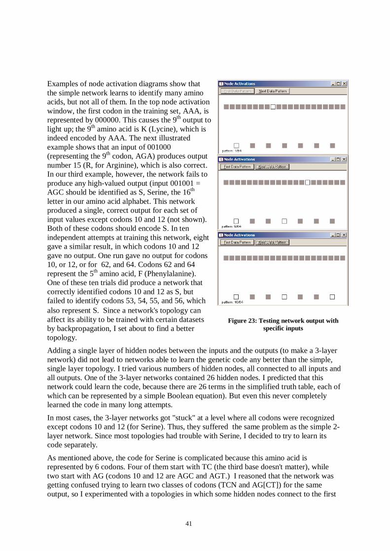
41

Examples of node activation diagrams show thatthe simple network learns to identify many aminoacids, but not all of them. In the top node activationwindow, the first codon in the training set, AAA, isrepresented by 000000. This causes the 9th output tolight up; the 9th amino acid is K (Lycine), which isindeed encoded by AAA. The next illustratedexample shows that an input of 001000(representing the 9th codon, AGA) produces outputnumber 15 (R, for Arginine), which is also correct.In our third example, however, the network fails toproduce any high-valued output (input 001001 =AGC should be identified as S, Serine, the 16th

letter in our amino acid alphabet. This networkproduced a single, correct output for each set ofinput values except codons 10 and 12 (not shown).Both of these codons should encode S. In tenindependent attempts at training this network, eightgave a similar result, in which codons 10 and 12gave no output. One run gave no output for codons10, or 12, or for 62, and 64. Codons 62 and 64represent the 5th amino acid, F (Phenylalanine).One of these ten trials did produce a network thatcorrectly identified codons 10 and 12 as S, butfailed to identify codons 53, 54, 55, and 56, whichalso represent S. Since a network's topology canaffect its ability to be trained with certain datasetsby backpropagation, I set about to find a bettertopology.

Adding a single layer of hidden nodes between the inputs and the outputs (to make a 3-layernetwork) did not lead to networks able to learn the genetic code any better than the simple,single layer topology. I tried various numbers of hidden nodes, all connected to all inputs andall outputs. One of the 3-layer networks contained 26 hidden nodes. I predicted that thisnetwork could learn the code, because there are 26 terms in the simplified truth table, each ofwhich can be represented by a simple Boolean equation). But even this never completelylearned the code in many long attempts.

In most cases, the 3-layer networks got "stuck" at a level where all codons were recognizedexcept codons 10 and 12 (for Serine). Thus, they suffered the same problem as the simple 2-layer network. Since most topologies had trouble with Serine, I decided to try to learn itscode separately.

As mentioned above, the code for Serine is complicated because this amino acid isrepresented by 6 codons. Four of them start with TC (the third base doesn't matter), whiletwo start with AG (codons 10 and 12 are AGC and AGT.) I reasoned that the network wasgetting confused trying to learn two classes of codons (TCN and AG[CT]) for the sameoutput, so I experimented with a topologies in which some hidden nodes connect to the first

Figure 23: Testing network output withspecific inputs

42

four inputs (for the first two bases), and some hidden nodes connect to only the last twoinputs (for the base in the "wobble" position).

NODES:nodes = 15inputs = 6outputs = 1output nodes are 15CONNECTIONS:groups = 01-15 from 01-4 from i1-i45-6 from i5-i67-10 from 1-411-14 from 5-615 from 7-14SPECIAL:

Figure 24: A topology for learning Serine

The most reliable Serine-learning network I was able to identify has two hidden layers (4layers total). I will describe the nodes using Tlearn's conventions; input nodes are called i1through i6; the first layer of hidden nodes are 1 through 6, the second hidden layer has sevennodes numbered 7 through 14, and node 15 is the output. The first four hidden nodes takeinput from all of the first four inputs together, and give output to all of the first four nodes inthe next layer. Nodes 5 and 6 in the first hidden layer both take input from both inputs 5 and6, and send output to the set of nodes 11-14 on the second hidden layer. All the nodes in thesecond hidden layer send results to the output node. The Tlearn Network Architecturediagram and configuration file are shown below.

This topology was very successful in learning the Serine values from the truth table. In 40trials (each with a maximum of 100000 sweeps, learning rate = 1, momentum = 0.2), itlearned the Serine output correctly each time.

In theory, a single hidden layer should be sufficient to represent any function (I think this iswhy Tlearn diagrams the hidden nodes all on a single level). However, I was never able todevise a topology with a single hidden layer that could learn the Serine values.

43

Table 9: Four-layer topology can learn the genetic code, but doesn't always

A. B. C.

D. E. F.

G. H. I.

J.

Network: training Optionslearning rate: 0.1momentum: 0Train in random sequence.

K.

Some of the stuck runs goon and on...

L. Tlearn configuration file.NODES:nodes = 37inputs = 6outputs = 21output nodes are 17-37CONNECTIONS:groups = 01-16 from 01-4 from i1-i45-6 from i5-i67-12 from 1-413-16 from 5-617-37 from 7-16SPECIAL:

Testing this topology on other amino acids showed that it could learn them also, so it is notrestricted to learning Serine. I then added more outputs to test whether similar topologiescould learn the entire genetic code at once. This is very similar to the four layer networkdescribed above for learning Serine, except it has a few more nodes added to each of the twogroups in the second hidden layer, and the second hidden layer connects to all of the 21outputs. Of ten trials using this topology, the network learned the genetic code in two (D andF in the table).

44

Figure 25: Four-layer topology capable of learning the genetic code, sometimes.

In a last-ditch attempt at finding a topology that can learn the genetic code reliably, Ireasoned that if a single layer can learn all amino acids but Serine, and if the four-layertopology described above can learn Serine alone, then I should be able to construct a hybridtopology that treats Serine as a special case. This is shown below, along with its Tlearnconfiguration.

NODES:nodes = 34inputs = 6outputs = 21output nodes are14-34CONNECTIONS:groups = 01-34 from 01-4 from i1-i45-6 from i5-i67-10 from 1-411-13 from 5-629 from 7-1314-28 from i1-i630-34 from i1-i6SPECIAL:

Figure 26: The most effective topology for learning the genetic code treats Serine as a special case.

The topology treating Serine as a special case was very effective for learning the geneticcode. In 20 of 20 trials, it succeeded in learning the entire code in < 200000 sweeps (learningrate = 1, momentum=0.5).

45

A.4. Implications of Experiments on Topology

The genetic code is a toy problem, in that it can be completely described in a look-up table,so neural network pattern finding does not reveal anything new. It is a suitable exampleproblem as an application of artificial neural networks in bioinformatics only in that it mayhelp students become familiar with the concept that the genetic code is in fact a lookup table(the term is commonly misused to mean "genome", more or less, in the popular press.)

These experiments demonstrate that choice of a suitable neural network topology isextremely important in learning certain Boolean functions, such as the genetic code. Onetopology (treating serine as a special case) was found which is quite reliable for learning thegenetic code. This topology is not very satisfying in a general sense, however, because it ishighly specialized for this problem. A general machine learning solution, either for findingappropriate topologies, or for better training of standard topologies, would be moreinteresting. This function could serve as a good example system for experimenting withapproaches such as using genetic algorithms for neural network topology identification; thisis called "neuroevolution"2.

Because of the complexity and specialized nature of the only topology I found that couldlearn the genetic code reliably, I chose not to attempt this problem in the Exceldemonstration. The spreadsheet would be rather complicated, and conducting the requirednumber of training steps with so many nodes seemed impractical. Instead, the demonstrationuses the classic XOR function..

2 See also the Wikipedia article on "Neuroevolution", http://en.wikipedia.org/wiki/Neuroevolution

46

Glossary

3' end: the end of a DNA sequence where the free 3' hydroxy group is found.

5' end: the end of a DNA chain where the free 5' phosphate group is normally located. DNAsequences are normally written with the 5' end on the left.

A: the abbreviation for adenine in a nucleic acid sequence.

adenine: a purine base found in DNA and RNA. Pairs with T in normal Watson-Crickpairing.

amino acid: one of the basic building blocks of proteins. There are twenty "normal" aminoacids commonly found in proteins. This means that the sequences of most proteinscan be described using a twenty-character alphabet.

amino terminus: the beginning of a protein chain, where the free amino group is located.Proteins are synthesized in the amino to carboxy terminus direction by ribozymes.The amino terminus of a protein is encoded by sequences toward the 5' end of thegene for that protein. By convention, protein sequences are written with the aminoterminus on the left.

antiparallel: strands running alongside one another but having opposite orientations.

artificial neural network: a set of artificial neurons connected with a certain topology.

base pairing: the hybridization of complementary nucleotides. A normally pairs with T, andC pairs with G.

Bayes' theorem: P(A|B) = P(B|A) * P(A) / P(B)

BLOSUM: "Blocks Substitution Matrix", one of the classic types of scoring tables for aminoacid comparisons.

C: see cytosine.

carboxy terminus: the end of a protein chain that has a free carboxy group. See aminoterminus.

central dogma: the concept that genetic information flows from long-term storage in DNA,to short term storage in mRNA, to proteins capable of carrying out biologicalfunction. There are known exceptions to this pattern, such as the reversetranscriptases of certain viruses (retroviruses) that copy information from RNA toDNA. Also, some organisms, notably viruses, keep long term genetic information inRNA molecules rather than DNA.

chloroplast: the subcellular organelle of plants wherein photosynthesis occurs.

chromosome: organized structures containing the major portion of an organism's DNA.Eukaryotic chromosomes are located in the nucleus.

classification: the process of assigning instances to categories.

codon: a triplet of three consecutive nucleotide bases encoding a particular amino acid.

complementary: having have G match with C, and A match with T.

C-terminus: see carboxy terminus.

47

cytosine: a pyrimidine base found in DNA and RNA. Pairs with G in normal Watson-Crickpairing.

denaturation: any process that causes the normal three dimensional structure of a protein tobe disrupted. Denaturation can have drastic effects on the properties of proteins.Cooking egg whites, for example, causes the albumin proteins to denature, and to losetheir solubility in water, and denatured enzymes lose their catalytic activities.

deoxyribonucleotide: any of the monomers from which DNA polymers are constructed.Deoxyribnucleotides consist of a nucleotide base (A, C, G, or T) connected to adeoxyribose sugar molecule, which has a phosphate group that can form aphosphodiester bond with the previous monomer in the chain.

DNA polymerase: any enzyme that produces DNA could be called a DNA polymerase. Thereare many types of DNA-producing enzymes. For example, an enzyme involved inDNA replication might be called a DNA-directed DNA polymerase. A reversetranscriptase could be called an RNA directed DNA polymerase. There are alsoenzymes that can produce DNA molecules without a template.

DNA: deoxyribonucleic acid. In most organisms, this is the genetic material.

edit distance: a similarity metric for comparing two sequences which is scored by the numberof edits (insertions, deletions, and substitutions) required to convert one sequence intothe other. Each editing operation may have its own score, which may be contained ina scoring table.

enzyme: a biological molecule capable of acting as a catalyst for a particular biochemicalreaction. Most enzymes are proteins, but some include RNA, and some are purelyRNA ("ribozymes").

eukaryotic: a type of organism having nucleate cells. Organisms without cell nuclei, such asbacteria, are called prokaryotic.

extrachromosomal: being located outside of a chromosome. Mitochondrial genes are said tobe extrachromosomal, for instance.

G: see guanine.

gene: a region of genetic material that carries the information for a specific trait. This is abroad definition, since "trait" could mean many things. Simple examples of usuallyencode a particular protein, including promoter regions, exons, etc. However, somegenes encode RNA molecules that are not translated to proteins (such as tRNAs),some act as regulatory regions, and some may have no known biological effect, aswith many of the "genes" for some markers used to distinguish individuals in forensicinvestigations, for example.

genetic code: a mapping of codons to amino acids. A standard genetic code is used by mostorganisms.

genome: the content of all of an organism's chromosomes.

guanine: a purine base found in DNA and RNA. Normally pairs with C in double-strandednucleic acids.

Hierarchical Clustering: grouping of instances into a tree-like structure showing howclosely they are related to one another. Clustering is commonly done usingunsupervised machine learning methods.

48

hybridization: annealing of complementary strands, especially strands with different origins(such as a target and a probe).

initiation codon: the first triplet in a reading frame.

MAP hypothesis: see "maximum aposteriori hypothesis"

maximum aposteriori hypothesis: the hypothesis with the highest posterior probability.

mitochondria: a subcellular organelle found in most nucleated cells. Mitochondria arecentrally important in the process of respiration.

naïve Bayes classifier: a classifier based on Bayes' theorem in which the simplifyingassumption is made that the probabilities of all attribute values are independent of oneanother.

N-terminus: see amino terminus.

Operational Taxonomic Unit: (OTU) a node in an evolutionary tree.

PAM: "Percent Acceptable Mutations", one of the classic types of scoring tables for aminoacid comparisons.

pathway: a series of biochemical reactions leading from one or more starting materials tometabolic products. The steps in a pathway are usually catalyzed by enzymes.

PCR: see "polymerase chain reaction".

peptide: a short protein chain. Peptides typically do not have enzymatic activity, since theyare too small to form the molecular machines we call enzymes. Many peptides havebiological activities as neurotransmitters or immunological targets. The name refersto the type of amino-ester bonds used to join amino acids together.

polymerase chain reaction: (PCR) a process by which targeted regions of DNA moleculescan be reproduced under experimental conditions. It is a recursive application orprimer extension.

polypeptide: a chain of amino acids joined by peptide bonds (a protein chain).

posterior probability: the probability of a hypothesis, given the observed data.

primary structure: the sequence of a protein chain. This can be though of as a one-dimensional description of the protein.

primer: a single-stranded nucleic acid molecule (usually a synthetic oligonucleotide) thathybridizes to a template molecule and serves to initiate template-directed synthesis byDNA polymerase.

prior probability: the assumed probability of a hypothesis before observations are made.

promoter : a region of a gene directing RNA polymerase activity at a particular transcriptionstart site.

protein: a polymer of amino acids linked by peptide bonds. Many proteins have biologicalfunctions that depend on their three-dimensional structures. A principle determinantof how one or more protein chains of amino acids folds into a three dimensionalstructure is the sequence of amino acids in the chains. The process of protein foldingis an important step in converting one-dimensional sequence information (as stored inDNA) into biological activities.

49

quaternary structure: the association of multiple protein chains into a single three-dimensional structure.

reading frame: The modulus or register in which a nucleic acid sequence is or could betranslated into protein. A strand of DNA has three possible reading frames, and itscomplementary strand ahs three more.

replication: the process of reproducing molecules or simple organisms (viruses are said toreplicate, for example).

reverse complement: the sequence of the strand that would pair exactly with a given strand.Matching strands must be both complementary and antiparallel.

ribozome: a macromolecular assembly responsible for translation of RNA sequences toproteins.

RNA polymerase: an enzyme that catalyzes the production of polymers of ribonucleic acid.

RNA: ribonucleic acid. Similar in structure to DNA, RNA is typically less stable. RNAperforms many vital functions in living things. Some types of RNA molecules(mRNA) act as messengers in the process of protein production. Others (tRNA)couple to activated amino acids to help match them to their codons. Ribosomescontain large amounts of structural rRNA. Other RNA molecules are intimatelyinvolved in other enzymatic functions, such as splicing.

secondary structure: local three-dimensional structure within a polymer chain. Commonsecondary structures in proteins include the alpha helix, the beta pleated sheet, and"turns" or "coils". Prediction of secondary structure from a protein sequence is easierthat predicting its complete three-dimensional structure, and is widely considered tobe a first step in structure prediction.

sequence: the order of monomers within a polymer, or of characters within a string. Geneticinformation is contained in the sequence of bases in DNA.

squashing function: a differentiable function that maps the output of an artificial neuron intoa finite range.

stochastic gradient descent: an approach to training a neural network wherein errors areback-propagated for each individual example, rather than for the entire training set atonce.

supervised learning: the process by which a program induces rules for classifying instances,based on pre-classified examples given in a training set.

synthetic oligonucleotide: a short strand of DNA created using techniques of organicchemistry.

T: see thymine.

tertiary structure: the three dimensional arrangement of a single protein chain.

thymine: a pyrimidine base found in DNA. (The thymines of DNA sequences are transcribedinto uracils in RNA). Normally pairs with A.

training set: a group of pre-classified examples that can be used with machine learningapproaches.

transcription factor: a protein that interacts with a gene sequence to control RNApolymerase activity at that gene.

50

transcription: the process of copying information from DNA to RNA. This is done by DNA-dependant RNA polymerase.

translation: the process of creating a protein molecule based on the sequence informationcontained in a molecule of messenger RNA.

uracil : the pyrimidine base that takes the place of thymine in RNA.

virus: an acellular infectious particle that replicates within cells of a host organism.

51

Bibliography

Alizadeh, A.A., Eisen, M.B., Davis, R.E., Ma, C., Lossos, I.S., Rosenwald, A., Boldrick,J.C., Sabet, H., Tran, T., Yu, X., Powell, J.I., Yang, L., Marti, G.E., Moore, T.,Hudson, J., Lu, L., Lewis, D.B., Tibshirani, R., Sherlock, G., Chan, W.C., Greiner,T.C., Weisenburger, D.D., Armitage, J.O., Warnke, R., Staudt, L.M. (2000). DistinctTypes of Diffuse Large B-Cell Lymphoma Identified by Gene Expression Profiling.Nature 403, 503-11. http://rana.lbl.gov/papers/Alizadeh_Nature_2000.pdf

Altman, R. (1998) A curriculum for bioinformatics: the time is ripe (editorial).Bioinformatics 14(7):549-550. http://www-smi.stanford.edu/pubs/SMI_Reports/SMI-98-0744.pdf

Delamarche, C. (2000) Color and Graphic Display (CGD): Programs for Multiple SequenceAlignment Analysis in Spreadsheet Software. BioTechniques 29:100-107.

Durbin, R., Eddy, S., Krogh, A., and Mitchison, G. (1998) Biological Sequence Analysis:probabilistic models of proteins and nucleic acids. Cambridge University Oress.

Eisen, M.B., Spellman, P.T., Brown, P.O. and Botstein, D. (1998). Cluster Analysis andDisplay of Genome-Wide Expression Patterns. Proc Natl Acad Sci U S A 95, 14863-8.

Felsenstein, J. (1989) PHYLIP - Phylogeny Inference Package (Version 3.2). Cladistics 5:164-166.

Felsenstein, J. (2004) PHYLIP (Phylogeny Inference Package) version 3.6. Distributed bythe author. Department of Genome Sciences, University of Washington, Seattle.

Gentleman, R.C., Carey, V.J., Bates, D.M., Bolstad, B., Dettling, M., Dudoit, S., Ellis, B.,Gautier, L., Ge, Y., Gentry, J., Hornik, K., Hothorn, T., Huber, W., Iacus, S., Irizarry,R., Leisch, F., Li, C., Maechler, M., Rossini, A.J., Sawitzki, G., Smith, C., Smyth, G.,Tierney, L., Yang, J.Y., and Zhang, J. (2004) Bioconductor: open softwaredevelopment for computational biology and bioinformatics. Genome Biol.;5(10):R80. http://genomebiology.com/2004/5/10/R80

Graham, P. (2002) A Plan for Spam. Retrieved December 4th, 2004 fromhttp://www.paulgraham.com/spam.html

Gusfield, D. (1997) Algorithms on Strings, Trees, and Sequences. Cambridge UniversityPress.

Han, B., and Tashjian, A. H. (1998) User-Friendly and Versatile Software for Analysis ofProtein Hydrophobicity. BioTechniques 25:256-263.

Higgins D., Thompson J., Gibson T.Thompson J.D., Higgins D.G., Gibson T.J. (1994).CLUSTAL W: improving the sensitivity of progressivemultiple sequence alignmentthrough sequence weighting,position-specific gap penalties and weight matrix choice.Nucleic Acids Res. 22:4673-4680.http://www.pubmedcentral.nih.gov/picrender.fcgi?tool=EBI&pubmedid=7984417&action=stream&blobtype=pdf

McEwan, N. R., and Gatherer, D. (1998) Adaptation of Standard Spreadsheet Software forthe Analysis of DNA Sequences. BioTechniques 24:131-138.

Mitchell, T.M. (1997) Machine Learning. WCB/McGraw-Hill.

52

Monroe, W.T., and Haselton, F.R. (2003) Molecular Beacon Sequence Design Algorithm.BioTechniques 34:68-73.

Needleman, S.B. and Wunsch, C.D. (1970) A general method applicable to the search forsimilarities in the amino acid sequence of two proteins. Journal of Molecular Biology48:443-453.

O'Neill, M.C., and Song, L. (2003) Neural network analysis of lymphoma microarray data:prognosis and diagnosis near-perfect. BMC Bioinformatics 4:13.http://www.biomedcentral.com/1471-2105/4/13

Sakakibara, Y., Brown, M., Hughey, R., Mian, I.S., Sjolander, K., Underwood, R.C.,Haussler, D. (1994) Stochastic context-free grammars for tRNA modeling. NucleicAcids Research. 22(23):5112-20.http://www.pubmedcentral.nih.gov/articlerender.fcgi?tool=pubmed&pubmedid=7800507

Schageman, J.J., Basit, M., Gallardo, T.D., Garner, H.R., and Shohet, R.V. (2002) MarC-V: aspreadsheet-based tool for analysis, normalization, and visualization of single cDNAmicroarray experiments. BioTechniques 32:338-344

Schütz, E., and von Ahsen, N. (1999) Spreadsheet Software for Thermodynamic MeltingPoint Prediction of Oligonucleotide Hybridization with and without Mismatches.BioTechniques 27:1218-1224.

Setubal, J. and Meidanis, J. (1997) Introduction to Computational Molecular Biology. PWSPublishing Company, Boston.

Shaw, G. (1997) "Spreadsheets in Molecular Biology". Chapter 7 of "Spreadsheets inScience and Engineering", pages 203-228, Editor Gordon Filby, Springer-Verlag,Heidelberg, Germany.

Smith, T.F. and Waterman, M.S. (1981) Identification of common molecular subsequences.Journal of Molecular Biology 147:195-197.

Snow C.D., Nguyen, H., Pande, V.S., and Gruebele, M. ( 2002) Absolute comparison ofsimulated and experimental protein-folding dynamics. Nature 420(6911):102-10.http://vsp27.stanford.edu/papers/SnowNature2002.pdf

Stowe, R. P., and Pierson, D. L. (1996) Spreadsheet Macro for Setting Up PCR Assay Tubes.BioTechniques 20:1088-1089.

Tobler, J.B., Molla, M.N., Nuwaysir, E.F., Green, R.D., Shavlik, J.W. (2002) Evaluatingmachine learning approaches for aiding probe selection for gene-expression arrays.Bioinformatics. 2002;18 Suppl 1:S164-71.http://www.ncbi.nlm.nih.gov/entrez/query.fcgi?cmd=Retrieve&db=pubmed&dopt=Abstract&list_uids=12169544

von Neumann, J. (1958) The Computer and the Brain, Yale University Press, New Haven.

Wang, D., Coscoy, L., Zylberberg, M., Avila, P.C., Boushey, H.A., Ganem, D., and DeRisi,J.L. (2002) Microarray-based detection and genotyping of viral pathogens.Proceedings of the National Acadamy of Sciences USA , 99(24):15687-92.http://derisilab.ucsf.edu/publications/pdfs/VirusChip.pdf

Wang, D., Urisman, A., Liu, Y.-T., Springer, M., Ksiazek, T.G., Erdman, D.D., Mardis, E.R.,Hickenbotham, M., Magrini, V., Eldred, J., Latreille, J.P., Wilson, R.K., Ganem, D.,

53

and DeRisi, J.L. (2003) Viral discovery and sequence recovery using DNAmicroarrays. PLoS Biology, 1(2):E2 http://www.plosbiology.org/archive/1545-7885/1/2/pdf/10.1371_journal.pbio.0000002-L.pdf

Weir, B.S. (1996) Genetic Data Analysis II: Methods for discrete population genetic data,Sinauer Associates, Sunderland MA

Wu, S., and Manber, U. (1991) Fast text searching with errors. University of ArizonaTechnical Report TR 91-11. ftp.cs.arizona.edu/agrep/agrep.ps.1

Zeeberg, B.R., Riss, J., Kane, D.W., Bussey, K.J., Uchio, E., Linehan, W.M., Barrett, J.C.,and Weinstein, J.N. (2004) Mistaken Identifiers: Gene name errors can be introducedinadvertently when using Excel in bioinformatics. BioMed BMC Bioinformatics 5:80www.biomedcentral.com/1471-2105/5/80

54

Index

adenine, 2, 46amino acid, 1, 2, 3, 9, 11, 36, 39, 41, 43, 44,

46amino terminus, 2, 46antiparallel, 2, 46artificial neural network, 12, 19, 45, 46base pairing, 2, 46Bayes' theorem, 13, 22, 46BLOSUM, 9, 46carboxy terminus, 2, 46central dogma, 1, 46chloroplast, 46chromosome, 46classification, 5, 11, 13, 14, 22, 23, 27, 46clustering, 4, 11, 17, 47codon, 3, 36, 39, 41, 46, 48complementary, 2, 3, 46C-terminus, 2, 46cytosine, 2, 46, 47denaturation, 2, 47deoxyribonucleotide, 2, 47DNA, 1, 2, 3, 4, 9, 47, 49DNA polymerase, 1, 3, 47edit distance, 9, 11, 47enzyme, 47eukaryotic, 2, 47extrachromosomal, 2, 47gene, 3, 4, 5, 11, 22, 47genetic code, 3, 19, 36, 37, 38, 40, 41, 43, 44,

45, 47genome, 3, 45, 47guanine, 2, 47hybridization, 3, 4, 11, 22, 23, 48initiation codon, 3, 48machine learning, 5, 11, 12, 14, 22, 23, 24, 26,

28, 41, 49MAP hypothesis, 13, 48

maximum aposteriori hypothesis, 13, 48mitochondria, 2, 3, 48naïve Bayes classifier, 14, 48N-terminus, 2, 48Operational Taxonomic Unit, 17, 48PAM, 9, 48pathway, 48PCR, 4, 48peptide, 2, 48polymerase chain reaction, 4, 48polypeptide, 1, 2, 48posterior probability, 13, 48primary structure, 1, 48primer, 4, 48prior probability, 14, 48promoter, 3, 48protein, 1, 2, 3, 11, 36, 39, 48quaternary structure, 1, 49reading frame, 3, 36, 48, 49replication, 1, 3, 49reverse complement, 2, 3, 4, 49ribozome, 49RNA, 1, 3, 11, 49RNA polymerase, 1, 3, 49secondary structure, 1, 11, 49sequence, 1, 2, 3, 4, 9, 11, 15, 16, 22, 36, 43,

49squashing function, 12, 49stochastic gradient descent, 12, 49synthetic oligonucleotide, 4, 49tertiary structure, 1, 49thymine, 2, 3, 49transcription, 1, 3, 50transcription factor, 3, 49translation, 3, 50uracil, 3, 50virus, 11, 22, 26, 50