Binarized Neural Networks: Training Neural Networks with Weights andActivations Constrained to +1 or −1

Matthieu Courbariaux*1 MATTHIEU.COURBARIAUX@GMAIL.COMItay Hubara*2 ITAYHUBARA@GMAIL.COMDaniel Soudry3 DANIEL.SOUDRY@GMAIL.COMRan El-Yaniv2 RANI@CS.TECHNION.AC.ILYoshua Bengio1,4 YOSHUA.UMONTREAL@GMAIL.COM1Universite de Montreal2Technion - Israel Institute of Technology3Columbia University4CIFAR Senior Fellow*Indicates equal contribution. Ordering determined by coin flip.

AbstractWe introduce a method to train Binarized Neu-ral Networks (BNNs) - neural networks with bi-nary weights and activations at run-time. Attraining-time the binary weights and activationsare used for computing the parameters gradi-ents. During the forward pass, BNNs drasticallyreduce memory size and accesses, and replacemost arithmetic operations with bit-wise opera-tions, which is expected to substantially improvepower-efficiency. To validate the effectiveness ofBNNs we conduct two sets of experiments on theTorch7 and Theano frameworks. On both, BNNsachieved nearly state-of-the-art results over theMNIST, CIFAR-10 and SVHN datasets. Last butnot least, we wrote a binary matrix multiplicationGPU kernel with which it is possible to run ourMNIST BNN 7 times faster than with an unopti-mized GPU kernel, without suffering any loss inclassification accuracy. The code for training andrunning our BNNs is available on-line.

IntroductionDeep Neural Networks (DNNs) have substantially pushedArtificial Intelligence (AI) limits in a wide range of tasks,including but not limited to object recognition from im-ages (Krizhevsky et al., 2012; Szegedy et al., 2014), speechrecognition (Hinton et al., 2012; Sainath et al., 2013), sta-

tistical machine translation (Devlin et al., 2014; Sutskeveret al., 2014; Bahdanau et al., 2015), Atari and Go games(Mnih et al., 2015; Silver et al., 2016), and even abstractart (Mordvintsev et al., 2015).

Today, DNNs are almost exclusively trained on one ormany very fast and power-hungry Graphic ProcessingUnits (GPUs) (Coates et al., 2013). As a result, it is of-ten a challenge to run DNNs on target low-power devices,and substantial research efforts are invested in speedingup DNNs at run-time on both general-purpose (Vanhouckeet al., 2011; Gong et al., 2014; Romero et al., 2014; Hanet al., 2015) and specialized computer hardware (Farabetet al., 2011a;b; Pham et al., 2012; Chen et al., 2014a;b;Esser et al., 2015).

This paper makes the following contributions:

• We introduce a method to train Binarized-Neural-Networks (BNNs), neural networks with binaryweights and activations, at run-time, and when com-puting the parameters gradients at train-time (see Sec-tion 1).

• We conduct two sets of experiments, each imple-mented on a different framework, namely Torch7(Collobert et al., 2011) and Theano (Bergstra et al.,2010; Bastien et al., 2012), which show that it is pos-sible to train BNNs on MNIST, CIFAR-10 and SVHNand achieve nearly state-of-the-art results (see Section2).

• We show that during the forward pass (both at run-time and train-time), BNNs drastically reduce mem-ory consumption (size and number of accesses), and

arX

iv:1

602.

0283

0v3

[cs

.LG

] 1

7 M

ar 2

016

Binarized Neural Networks: Training Neural Networks with Weights and Activations Constrained to +1 or −1

replace most arithmetic operations with bit-wise oper-ations, which potentially lead to a substantial increasein power-efficiency (see Section 3). Moreover, a bi-narized CNN can lead to binary convolution kernelrepetitions; We argue that dedicated hardware couldreduce the time complexity by 60% .

• Last but not least, we programed a binary matrix mul-tiplication GPU kernel with which it is possible to runour MNIST BNN 7 times faster than with an unopti-mized GPU kernel, without suffering any loss in clas-sification accuracy (see Section 4).

• The code for training and running our BNNs is avail-able on-line (In both Theano framework 1 and Torchframework 2).

1. Binarized Neural NetworksIn this section, we detail our binarization function, showhow we use it to compute the parameters gradients, andhow we backpropagate through it.

1.1. Deterministic vs Stochastic Binarization

When training a BNN, we constrain both the weights andthe activations to either +1 or −1. Those two values arevery advantageous from a hardware perspective, as we ex-plain in Section 4. In order to transform the real-valuedvariables into those two values, we use two different bi-narization functions, as in (Courbariaux et al., 2015). Ourfirst binarization function is deterministic:

xb = Sign(x) =

{+1 if x ≥ 0,−1 otherwise, (1)

where xb is the binarized variable (weight or activation)and x the real-valued variable. It is very straightforward toimplement and works quite well in practice. Our secondbinarization function is stochastic:

xb =

{+1 with probability p = σ(x),−1 with probability 1− p, (2)

where σ is the “hard sigmoid” function:

σ(x) = clip(x+ 1

2, 0, 1) = max(0,min(1,

x+ 1

2)). (3)

The stochastic binarization is more appealing than the signfunction, but harder to implement as it requires the hard-ware to generate random bits when quantizing. As a re-sult, we mostly use the deterministic binarization function(i.e, the sign function), with the exception of activations attrain-time in some of our experiments.

1https://github.com/MatthieuCourbariaux/BinaryNet

2https://github.com/itayhubara/BinaryNet

1.2. Gradient Computation and Accumulation

Although our BNN training method uses binary weightsand activation to compute the parameters gradients, thereal-valued gradients of the weights are accumulated inreal-valued variables, as per Algorithm 1. Real-valuedweights are likely required for Stochasic Gradient Descent(SGD) to work at all. SGD explores the space of param-eters in small and noisy steps, and that noise is averagedout by the stochastic gradient contributions accumulated ineach weight. Therefore, it is important to keep sufficientresolution for these accumulators, which at first glance sug-gests that high precision is absolutely required.

Moreover, adding noise to weights and activations whencomputing the parameters gradients provide a form of reg-ularization that can help to generalize better, as previ-ously shown with variational weight noise (Graves, 2011),Dropout (Srivastava, 2013; Srivastava et al., 2014) andDropConnect (Wan et al., 2013). Our method of trainingBNNs can be seen as a variant of Dropout, in which insteadof randomly setting half of the activations to zero whencomputing the parameters gradients, we binarize both theactivations and the weights.

1.3. Propagating Gradients Through Discretization

The derivative of the sign function is zero almost every-where, making it apparently incompatible with backpropa-gation, since the exact gradient of the cost with respect tothe quantities before the discretization (pre-activations orweights) would be zero. Note that this remains true evenif stochastic quantization is used. Bengio (2013) studiedthe question of estimating or propagating gradients throughstochastic discrete neurons. They found in their experi-ments that the fastest training was obtained when using the“straight-through estimator,” previously introduced in Hin-ton (2012)’s lectures.

We follow a similar approach but use the version ofthe straight-through estimator that takes into account thesaturation effect, and does use deterministic rather thanstochastic sampling of the bit. Consider the sign functionquantization

q = Sign(r),

and assume that an estimator gq of the gradient ∂C∂q has

been obtained (with the straight-through estimator whenneeded). Then, our straight-through estimator of ∂C∂r is sim-ply

gr = gq1|r|≤1. (4)

Note that this preserves the gradient’s information and can-cels the gradient when r is too large. Not cancelling thegradient when r is too large significantly worsens the per-formance. The use of this straight-through estimator is il-lustrated in Algorithm 1. The derivative 1|r|≤1 can also be

Binarized Neural Networks: Training Neural Networks with Weights and Activations Constrained to +1 or −1

Algorithm 1 Training a BNN. C is the cost function forminibatch, λ - the learning rate decay factor andL the num-ber of layers. ◦ indicates element-wise multiplication. Thefunction Binarize() specifies how to (stochastically or de-terministically) binarize the activations and weights, andClip(), how to clip the weights. BatchNorm() specifies howto batch-normalize the activations, using either batch nor-malization (Ioffe & Szegedy, 2015) or its shift-based vari-ant we describe in Algorithm 3. BackBatchNorm() speci-fies how to backpropagate through the normalization. Up-date() specifies how to update the parameters when theirgradients are known, using either ADAM (Kingma & Ba,2014) or the shift-based AdaMax we describe in Algorithm4.Require: a minibatch of inputs and targets (a0, a

∗), pre-vious weights W , previous BatchNorm parameters θ,weights initialization coefficients from (Glorot & Ben-gio, 2010) γ, and previous learning rate η.

Ensure: updated weights W t+1, updated BatchNorm pa-rameters θt+1 and updated learning rate ηt+1.{1. Computing the parameters gradients:}{1.1. Forward propagation:}for k = 1 to L doW bk ← Binarize(Wk)

sk ← abk−1Wbk

ak ← BatchNorm(sk, θk)if k < L thenabk ← Binarize(ak)

end ifend for{1.2. Backward propagation:}{Please note that the gradients are not binary.}Compute gaL = ∂C

∂aLknowing aL and a∗

for k = L to 1 doif k < L thengak ← gabk ◦ 1|ak|≤1

end if(gsk , gθk)← BackBatchNorm(gak , sk, θk)gabk−1

← gskWbk

gW bk← g>ska

bk−1

end for{2. Accumulating the parameters gradients:}for k = 1 to L doθt+1k ← Update(θk, η, gθk)W t+1k ← Clip(Update(Wk, γkη, gW b

k),−1, 1)

ηt+1 ← ληend for

Algorithm 2 Shift based Batch Normalizing Transform,applied to activation x over a mini-batch. AP2(x) =sign(x) × 2round(log2|x|) is the approximate power-of-2 3,and�� stands for both left and right binary shift.Require: Values of x over a mini-batch: B = {x1...m};

Parameters to be learned: γ, βEnsure: {yi = BN(xi,γ, β)}µB ← 1

m

∑mi=1 xi {mini-batch mean}

C(xi)← (xi − µB) {centered input}σ2B← 1

m

∑mi=1(C(xi)��AP2(C(xi))){apx variance}

xi ← C(xi)�� AP2((√σ2B + ε)−1) {normalize}

yi ← AP2(γ)�� xi {scale and shift}

Algorithm 3 Shift based Batch Normalizing Transform,applied to activation (x) over a mini-batch. Where AP2 isthe approximate power-of-2 and �� stands for both leftand right binary shift.Require: Values of x over a mini-batch: B = {x1...m};

Parameters to be learned: γ, βEnsure: {yi = BN(xi,γ, β)}µB ← 1

m

∑mi=1 xi {mini-batch mean}

C(xi)← (xi − µB) {centered input}σ2B← 1

m

∑mi=1(C(xi)��AP2(C(xi))){apx variance}

xi ← C(xi)�� AP2((√σ2B + ε)−1) {normalize}

yi ← AP2(γ)�� xi {scale and shift}

seen as propagating the gradient through hard tanh, whichis the following piece-wise linear activation function:

Htanh(x) = Clip(x,−1, 1) = max(−1,min(1, x)). (5)

For hidden units, we use the sign function non-linearity toobtain binary activations, and for weights we combine twoingredients:

• Constrain each real-valued weight between -1 and 1,by projecting wr to -1 or 1 when the weight updatebrings wr outside of [−1, 1], i.e., clipping the weightsduring training, as per Algorithm 1. The real-valuedweights would otherwise grow very large without anyimpact on the binary weights.

• When using a weight wr, quantize it using wb =Sign(wr).

This is consistent with the gradient canceling when |wr| >1, according to Eq. 4.

3Hardware implementation of AP2 is as simple as extractingthe index of the most significant bit from the number’s binaryrepresentation.

Binarized Neural Networks: Training Neural Networks with Weights and Activations Constrained to +1 or −1

Algorithm 4 Shift based AdaMax learning rule (Kingma& Ba, 2014). g2t indicates the element-wise square gt ◦ gt.Good default settings are α = 2−10, 1−β1 = 2−3, 1−β2 =2−10 . All operations on vectors are element-wise. With βt1and βt2 we denote β1 and β2 to the power t.Require: Previous parameters θt−1 and their gradient gt,

and learning rate α.Ensure: Updated parameters θt{Biased 1st and 2nd raw moment estimates:}mt ← β1 ·mt−1 + (1− β1) · gtvt ← max(β2 · vt−1, |gt|){Updated parameters:}θt ← θt−1 − (α�� (1− β1)) · m�� v−1t )

Algorithm 5 Running a BNN. L is the number of layers.Require: a vector of 8-bit inputs a0, the binary weightsW b, and the BatchNorm parameters θ.

Ensure: the MLP output aL.{1. First layer:}a1 ← 0for n = 1 to 8 doa1 ← a1 + 2n−1 ×XnorDotProduct(an0 ,W

b1)

end forab1 ← Sign(BatchNorm(a1, θ1)){2. Remaining hidden layers:}for k = 2 to L− 1 doak ← XnorDotProduct(abk−1,W

bk)

abk ← Sign(BatchNorm(ak, θk))end for{3. Output layer:}aL ← XnorDotProduct(abL−1,W

bL)

aL ← BatchNorm(aL, θL)

1.4. Shift based Batch Normalization

Batch Normalization (BN) (Ioffe & Szegedy, 2015), accel-erates the training and also seems to reduces the overallimpact of the weights’ scale. The normalization noise mayalso help to regularize the model. However, at train-time,BN requires many multiplications (calculating the standarddeviation and dividing by it), namely, dividing by the run-ning variance (the weighted mean of the training set acti-vation variance). Although the number of scaling calcula-tions is the same as the number of neurons, in the case ofConvNets this number is quite large. For example, in theCIFAR-10 dataset (using our architecture), the first convo-lution layer, consisting of only 128×3×3 filter masks, con-verts an image of size 3×32×32 to size 3×128×28×28,which is two orders of magnitude larger than the number ofweights. To achieve the results that BN would obtain, weuse a shift-based batch normalization (SBN) technique. de-tailed in Algorithm 3. SBN approximates BN almost with-out multiplications. In the experiment we conducted we

did not observe accuracy loss when using the shift basedBN algorithm instead of the vanilla BN algorithm.

1.5. Shift based AdaMax

The ADAM learning rule (Kingma & Ba, 2014) also seemsto reduce the impact of the weight scale. Since ADAM re-quires many multiplications, we suggest using instead theshift-based AdaMax we detail in Algorithm 4. In the ex-periment we conducted we did not observe accuracy losswhen using the shift-based AdaMax algorithm instead ofthe vanilla ADAM algorithm.

1.6. First Layer

In a BNN, only the binarized values of the weights and ac-tivations are used in all calculations. As the output of onelayer is the input of the next, all the layers inputs are bi-nary, with the exception of the first layer. However, wedo not believe this to be a major issue. First, in computervision, the input representation typically has much fewerchannels (e.g, Red, Green and Blue) than internal repre-sentations (e.g, 512). As a result, the first layer of a Con-vNet is often the smallest convolution layer, both in termsof parameters and computations (Szegedy et al., 2014).

Second, it is relatively easy to handle continuous-valuedinputs as fixed point numbers, withm bits of precision. Forexample, in the common case of 8-bit fixed point inputs:

s = x · wb (6)

s =

8∑n=1

2n−1(xn · wb), (7)

where x is a vector of 1024 8-bit inputs, x81 is the mostsignificant bit of the first input, wb is a vector of 1024 1-bitweights, and s is the resulting weighted sum. This trick isused in Algorithm 5.

2. Benchmark ResultsWe conduct two sets of experiments, each based on a differ-ent framework, namely Torch7 (Collobert et al., 2011) andTheano (Bergstra et al., 2010; Bastien et al., 2012). Otherthan the framework, the two sets of experiments are verysimilar:

• In both sets of experiments, we obtain near state-of-the-art results with BNNs on MNIST, CIFAR-10 andthe SVHN benchmark datasets.

• In our Torch7 experiments, the activations are stochas-tically binarized at train-time, whereas in our Theanoexperiments they are deterministically binarized.

• In our Torch7 experiments, we use the shift-based BN

Binarized Neural Networks: Training Neural Networks with Weights and Activations Constrained to +1 or −1

Table 1. Classification test error rates of DNNs trained on MNIST (MLP architecture without unsupervised pretraining), CIFAR-10(without data augmentation) and SVHN.

Data set MNIST SVHN CIFAR-10Binarized activations+weights, during training and test

BNN (Torch7) 1.40% 2.53% 10.15%BNN (Theano) 0.96% 2.80% 11.40%Committee Machines’ Array (Baldassi et al., 2015) 1.35% - -

Binarized weights, during training and testBinaryConnect (Courbariaux et al., 2015) 1.29± 0.08% 2.30% 9.90%

Binarized activations+weights, during testEBP (Cheng et al., 2015) 2.2± 0.1% - -Bitwise DNNs (Kim & Smaragdis, 2016) 1.33% - -

Ternary weights, binary activations, during test(Hwang & Sung, 2014) 1.45% - -

No binarization (standard results)Maxout Networks (Goodfellow et al.) 0.94% 2.47% 11.68%Network in Network (Lin et al.) - 2.35% 10.41%Gated pooling (Lee et al., 2015) - 1.69% 7.62%

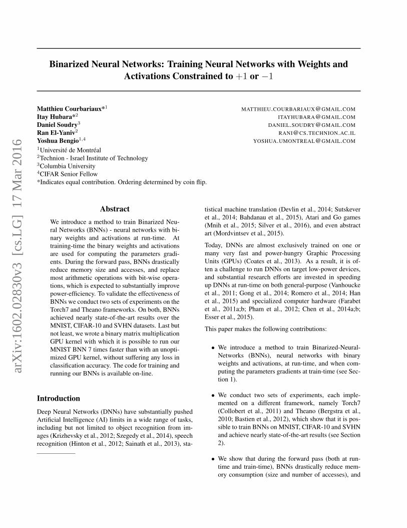
Figure 1. Training curves of a ConvNet on CIFAR-10 depend-ing on the method. The dotted lines represent the training costs(square hinge losses) and the continuous lines the correspondingvalidation error rates. Although BNNs are slower to train, theyare nearly as accurate as 32-bit float DNNs.

and AdaMax variants, which are detailed in Algo-rithms 3 and 4, whereas in our Theano experiments,we use vanilla BN and ADAM.

2.1. MLP on MNIST (Theano)

MNIST is an image classification benchmark dataset (Le-Cun et al., 1998). It consists of a training set of 60K anda test set of 10K 28 × 28 gray-scale images represent-ing digits ranging from 0 to 9. In order for this bench-mark to remain a challenge, we did not use any convo-lution, data-augmentation, preprocessing or unsupervisedlearning. The MLP we train on MNIST consists of 3 hid-den layers of 4096 binary units (see Section 1) and a L2-SVM output layer; L2-SVM has been shown to performbetter than Softmax on several classification benchmarks

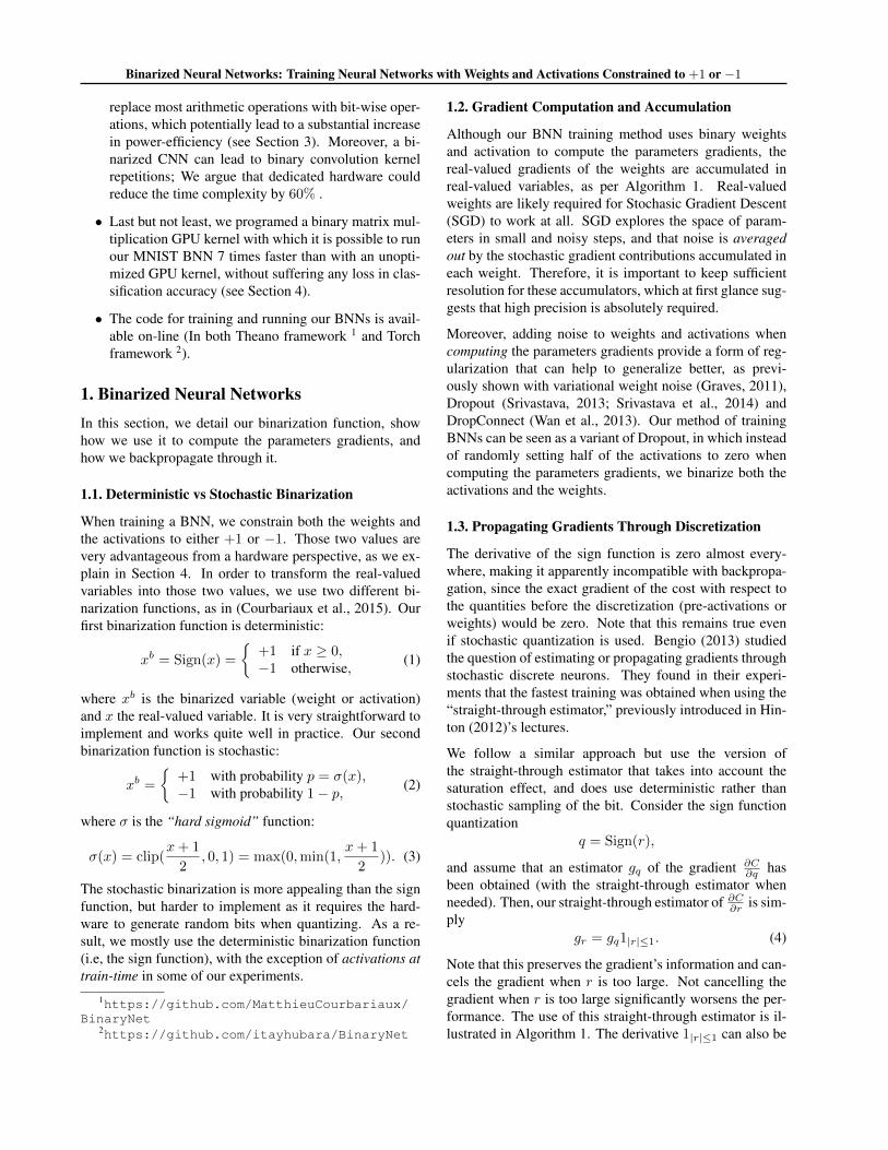
Figure 2. Binary weight filters, sampled from of the first convolu-tion layer. Since we have only 2k

2

unique 2D filters (where k isthe filter size), filter replication is very common. For instance, onour CIFAR-10 ConvNet, only 42% of the filters are unique.

(Tang, 2013; Lee et al., 2014). We regularize the modelwith Dropout (Srivastava, 2013; Srivastava et al., 2014).The square hinge loss is minimized with the ADAM adap-tive learning rate method (Kingma & Ba, 2014). We usean exponentially decaying global learning rate, as per Al-gorithm 1, and also scale the learning rates of the weightswith their initialization coefficients from (Glorot & Bengio,2010), as suggested by Courbariaux et al. (2015). We useBatch Normalization with a minibatch of size 100 to speedup the training. As is typical, we use the last 10K samplesof the training set as a validation set for early stopping andmodel selection. We report the test error rate associatedwith the best validation error rate after 1000 epochs (we donot retrain on the validation set). The results are reportedin Table 1.

2.2. MLP on MNIST (Torch7)

We use a similar architecture as in our Theano experiments,without dropout, and with 2048 binary units per layer in-stead of 4096. Additionally, we use the shift base AdaMax

Binarized Neural Networks: Training Neural Networks with Weights and Activations Constrained to +1 or −1

and BN (with a minibatch of size 100) instead of the vanillaimplementations, to reduce the number of multiplications.Likewise, we decay the learning rate by using a 1-bit rightshift every 10 epochs. The results are presented in Table 1.

2.3. ConvNet on CIFAR-10 (Theano)

CIFAR-10 is an image classification benchmark dataset. Itconsists of a training set of size 50K and a test set of size10K, where instance are 32 × 32 color images represent-ing airplanes, automobiles, birds, cats, deer, dogs, frogs,horses, ships and trucks. We do not use any preprocessingor data-augmentation (which can really be a game changerfor this dataset (Graham, 2014)). The architecture of ourConvNet is the same architecture as ?’s except for the bi-narization of the activations. Courbariaux et al. (2015)’sarchitecture is itself mainly inspired by VGG (Simonyan& Zisserman, 2015). The square hinge loss is minimizedwith ADAM. We use an exponentially decaying learningrate, as we did for MNIST. We scale the learning rates ofthe weights with their initialization coefficients from (Glo-rot & Bengio, 2010). We use Batch Normalization with aminibatch of size 50 to speed up the training. We use thelast 5000 samples of the training set as a validation set. Wereport the test error rate associated with the best validationerror rate after 500 training epochs (we do not retrain onthe validation set). The results are presented in Table 1 andFigure 1.

2.4. ConvNet on CIFAR-10 (Torch7)

We use the same architecture as in our Theano experiments.We apply shift-based AdaMax and BN (with a minibatchof size 200) instead of the vanilla implementations to re-duce the number of multiplications. Likewise, we decaythe learning rate by using a 1-bit right shift every 50 epochs.The results are presented in Table 1 and Figure 1.

2.5. ConvNet on SVHN

SVHN is also an image classification benchmark dataset. Itconsists of a training set of size 604K examples and a testset of size 26K, where instances are 32 × 32 color imagesrepresenting digits ranging from 0 to 9. In both sets ofexperiments, we follow the same procedure used for theCIFAR-10 experiments, with a few notable exceptions: weuse half the number of units in the convolution layers, andwe train for 200 epochs instead of 500 (because SVHN is amuch larger dataset than CIFAR-10). The results are givenin Table 1.

3. Very Power Efficient in Forward PassComputer hardware, be it general-purpose or specialized,is composed of memories, arithmetic operators and control

Table 2. Energy consumption of multiply-accumulations(Horowitz, 2014)

Operation MUL ADD8bit Integer 0.2pJ 0.03pJ32bit Integer 3.1pJ 0.1pJ16bit Floating Point 1.1pJ 0.4pJ32tbit Floating Point 3.7pJ 0.9pJ

Table 3. Energy consumption of memory accesses (Horowitz,2014)

Memory size 64-bit memory access8K 10pJ32K 20pJ1M 100pJDRAM 1.3-2.6nJ

logic. During the forward pass (both at run-time and train-time), BNNs drastically reduce memory size and accesses,and replace most arithmetic operations with bit-wise op-erations, which might lead to a great increase in power-efficiency. Moreover, a binarized CNN can lead to binaryconvolution kernel repetitions, and we argue that dedicatedhardware could reduce the time complexity by 60% .

3.1. Memory Size and Accesses

Improving computing performance has always been and re-mains a challenge. Over the last decade, power has been themain constraint on performance (Horowitz, 2014). This iswhy much research effort has been devoted to reducing theenergy consumption of neural networks. Horowitz (2014)provides rough numbers for the computations’ energy con-sumption (the given numbers are for 45nm technology) assummarized in Tables 2 and 3. Importantly, we can seethat memory accesses typically consume more energy thanarithmetic operations, and memory access’ cost augmentswith memory size. In comparison with 32-bit DNNs, BNNsrequire 32 times smaller memory size and 32 times fewermemory accesses. This is expected to reduce energy con-sumption drastically (i.e., more than 32 times).

3.2. XNOR-Count

Applying a DNN mainly consists of convolutions and ma-trix multiplications. The key arithmetic operation of deeplearning is thus the multiply-accumulate operation. Artifi-cial neurons are basically multiply-accumulators comput-ing weighted sums of their inputs. In BNNs, both the ac-tivations and the weights are constrained to either −1 or+1. As a result, most of the 32-bit floating point multiply-accumulations are replaced by 1-bit XNOR-count opera-tions. This could have a big impact on deep learning ded-icated hardware. For instance, a 32-bit floating point mul-tiplier costs about 200 Xilinx FPGA slices (Govindu et al.,2004; Beauchamp et al., 2006), whereas a 1-bit XNOR gate

Binarized Neural Networks: Training Neural Networks with Weights and Activations Constrained to +1 or −1

only costs a single slice.

3.3. Exploiting Filter Repetitions

When using a ConvNet architecture with binary weights,the number of unique filters is bounded by the filter size.For example, in our implementation we use filters of size3 × 3, so the maximum number of unique 2D filters is29 = 512. However, this should not prevent expandingthe number of feature maps beyond this number, since theactual filter is a 3D matrix. Assuming we have M` fil-ters in the ` convolutional layer, we have to store a 4Dweight matrix of size M` ×M`−1 × k × k. Consequently,the number of unique filters is 2k

2M`−1 . When necessary,we apply each filter on the map and perform the requiredmultiply-accumulate (MAC) operations (in our case, usingXNOR and popcount operations). Since we now have bi-nary filters, many 2D filters of size k×k repeat themselves.By using dedicated hardware/software, we can apply onlythe unique 2D filters on each feature map and sum the re-sult wisely to receive each 3D filter’s convolutional result.Note that an inverse filter (i.e., [-1,1,-1] is the inverse of[1,-1,1]) can also be treated as a repetition; it is merely amultiplication of the original filter by -1. For example, inour ConvNet architecture trained on the CIFAR-10 bench-mark, there are only 42% unique filters per layer on av-erage. Hence we can reduce the number of the XNOR-popcount operations by 3.

4. Seven Times Faster on GPU at Run-TimeIt is possible to speed up GPU implementations of BNNs,by using a method sometimes called SIMD (single in-struction, multiple data) within a register (SWAR). Thebasic idea of SWAR is to concatenate groups of 32 bi-nary variables into 32-bit registers, and thus obtain a 32-times speed-up on bitwise operations (e.g, XNOR). UsingSWAR, it is possible to evaluate 32 connections with only3 instructions:

a1+ = popcount(xnor(a32b0 , w32b1 )), (8)

where a1 is the resulting weighted sum, and a32b0 and w32b1

are the concatenated inputs and weights. Those 3 instruc-tions (accumulation, popcount, xnor) take 1 + 4 + 1 = 6clock cycles on recent Nvidia GPUs (and if they were to be-come a fused instruction, it would only take a single clockcycle). Consequently, we obtain a theoretical Nvidia GPUspeed-up of factor of 32/6 ≈ 5.3. In practice, this speed-upis quite easy to obtain as the memory bandwidth to compu-tation ratio is also increased by 6 times.

In order to validate those theoretical results, we programedtwo GPU kernels:

• The first kernel (baseline) is a quite unoptimized ma-

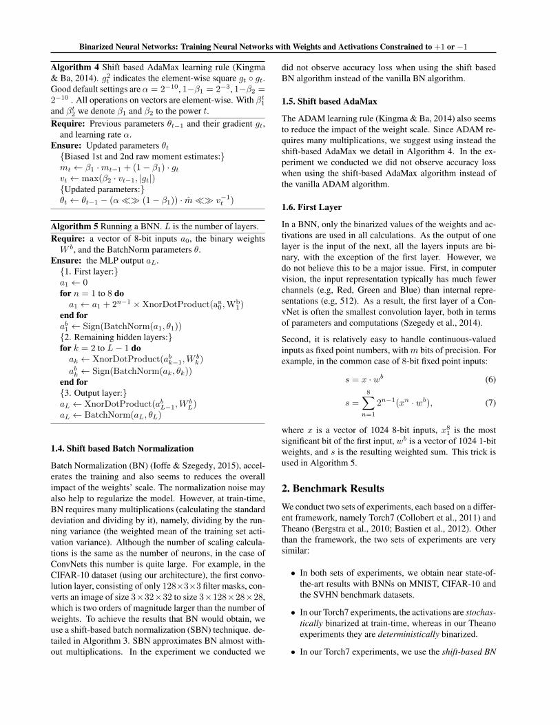
Figure 3. The first three columns represent the time it takes toperform a 8192× 8192× 8192 (binary) matrix multiplication ona GTX750 Nvidia GPU, depending on which kernel is used. Wecan see that our XNOR kernel is 23 times faster than our baselinekernel and 3.4 times faster than cuBLAS. The next three columnsrepresent the time it takes to run the MLP from Section 2 on thefull MNIST test set. As MNIST’s images are not binary, the firstlayer’s computations are always performed by the baseline ker-nel. The last three columns show that the MLP accuracy does notdepend on which kernel is used.

trix multiplication kernel.

• The second kernel (XNOR) is nearly identical to thebaseline kernel, except that it uses the SWAR method,as in Equation (8).

The two GPU kernels return identical outputs when theirinputs are constrained to−1 or +1 (but not otherwise). TheXNOR kernel is about 23 times faster than the baseline ker-nel and 3.4 times faster than cuBLAS, as shown in Figure3. Last but not least, the MLP from Section 2 runs 7 timesfaster with the XNOR kernel than with the baseline kernel,without suffering any loss in classification accuracy (seeFigure 3).

5. Discussion and Related WorkUntil recently, the use of extremely low-precision networks(binary in the extreme case) was believed to be highly de-structive to the network performance (Courbariaux et al.,2014). Soudry et al. (2014); ? showed the contrary byshowing that good performance could be achieved even ifall neurons and weights are binarized to ±1 . This wasdone using Expectation BackPropagation (EBP), a varia-tional Bayesian approach, which infers networks with bi-

Binarized Neural Networks: Training Neural Networks with Weights and Activations Constrained to +1 or −1

nary weights and neurons by updating the posterior distri-butions over the weights. These distributions are updatedby differentiating their parameters (e.g., mean values) viathe back propagation (BP) algorithm. Esser et al. (2015)implemented a fully binary network at run time using a verysimilar approach to EBP, showing significant improvementin energy efficiency. The drawback of EBP is that the bina-rized parameters were only used during inference.

The probabilistic idea behind EBP was extended in the Bi-naryConnect algorithm of Courbariaux et al. (2015). InBinaryConnect, the real-valued version of the weights issaved and used as a key reference for the binarization pro-cess. The binarization noise is independent between dif-ferent weights, either by construction (by using stochas-tic quantization) or by assumption (a common simplifica-tion; see Spang (1962). The noise would have little effecton the next neuron’s input because the input is a summa-tion over many weighted neurons. Thus, the real-valuedversion could be updated by the back propagated error bysimply ignoring the binarization noise in the update. Us-ing this method, Courbariaux et al. (2015) were the firstto binarize weights in CNNs and achieved near state-of-the-art performance on several datasets. They also arguedthat noisy weights provide a form of regularization, whichcould help to improve generalization, as previously shownin (Wan et al., 2013). This method binarized weights whilestill maintaining full precision neurons.

Lin et al. (2015) carried over the work of Courbariaux et al.(2015) to the back-propagation process by quantizing therepresentations at each layer of the network, to convertsome of the remaining multiplications into binary shifts byrestricting the neurons values of power-of-two integers. Linet al. (2015)’s work and ours seem to share similar charac-teristics . However, their approach continues to use full pre-cision weights during the test phase. Moreover, Lin et al.(2015) quantize the neurons only during the back propaga-tion process, and not during forward propagation.

Other research (Baldassi et al., 2015) showed that fully bi-nary training and testing is possible in an array of com-mittee machines with randomized input, where only oneweight layer is being adjusted. Judd et al. and Gonget al. aimed to compress a fully trained high precision net-work by using a quantization or matrix factorization meth-ods. These methods required training the network with fullprecision weights and neurons, thus requiring numerousMAC operations avoided by the proposed BNN algorithm.Hwang & Sung (2014) focused on a fixed-point neural net-work design and achieved performance almost identical tothat of the floating-point architecture. Kim et al. (2014)provided evidence that DNNs with ternary weights, usedon a dedicated circuit, consume very low power and canbe operated with only on-chip memory, at run time. Sung

et al. also indicated satisfactory empirical performance ofneural networks with 8-bit precision. Kim & Paris (2015)retrained neural networks with binary weights and activa-tions.

So far, to the best of our knowledge, no work has succeededin binarizing weights and neurons, at the inference phaseand the entire training phase of a deep network. This wasachieved in the present work. We relied on the idea that bi-narization can be done stochastically, or be approximatedas random noise. This was previously done for the weightsby Courbariaux et al. (2015), but our BNNs extend this tothe activations. Note that the binary activations are espe-cially important for ConvNets, where there are typicallymany more neurons than free weights. This allows highlyefficient operation of the binarized DNN at run time, andat the forward propagation phase during training. More-over, our training method has almost no multiplications,and therefore might be implemented efficiently in dedi-cated hardware. However, we have to save the value of thefull precision weights. This is a remaining computationalbottleneck during training, since it requires relatively highenergy resources. Novel memory devices might be used toalleviate this issue in the future; see e.g. (Soudry et al.).

ConclusionWe have introduced BNNs, DNNs with binary weights andactivations at run-time and when computing the parame-ters gradients at train-time (see Section 1). We have con-ducted two sets of experiments on two different frame-works, Torch7 and Theano, which show that it is possible totrain BNNs on MNIST, CIFAR-10 and SVHN, and achievenearly state-of-the-art results (see Section 2). Moreover,during the forward pass (both at run-time and train-time),BNNs drastically reduce memory size and accesses, and re-place most arithmetic operations with bit-wise operations,which might lead to a great increase in power-efficiency(see Section 3). Last but not least, we programed a binarymatrix multiplication GPU kernel with which it is possibleto run our MNIST MLP 7 times faster than with an unopti-mized GPU kernel, without suffering any loss in classifica-tion accuracy (see Section 4). Future works should explorehow to extend the speed-up to train-time (e.g., by binariz-ing some gradients), and also extend benchmark results toother models (e.g, RNN) and datasets (e.g, ImageNet).

AcknowledgmentsWe would like to express our appreciation to Elad Hoffer,for his technical assistance and constructive comments. Wethank our fellow MILA lab members who took the time toread the article and give us some feedback. We thank thedevelopers of Torch, (Collobert et al., 2011) a Lua based

Binarized Neural Networks: Training Neural Networks with Weights and Activations Constrained to +1 or −1

environment, and Theano (Bergstra et al., 2010; Bastienet al., 2012), a Python library which allowed us to easilydevelop a fast and optimized code for GPU. We also thankthe developers of Pylearn2 (Goodfellow et al., 2013) andLasagne (Dieleman et al., 2015), two Deep Learning li-braries built on the top of Theano. We thank Yuxin Wufor helping us compare our GPU kernels with cuBLAS. Weare also grateful for funding from CIFAR, NSERC, IBM,Samsung, and the Israel Science Foundation (ISF).

ReferencesBahdanau, Dzmitry, Cho, Kyunghyun, and Bengio, Yoshua. Neu-

ral machine translation by jointly learning to align and trans-late. In ICLR’2015, arXiv:1409.0473, 2015.

Baldassi, Carlo, Ingrosso, Alessandro, Lucibello, Carlo, Saglietti,Luca, and Zecchina, Riccardo. Subdominant Dense ClustersAllow for Simple Learning and High Computational Perfor-mance in Neural Networks with Discrete Synapses. PhysicalReview Letters, 115(12):1–5, 2015.

Bastien, Frederic, Lamblin, Pascal, Pascanu, Razvan, Bergstra,James, Goodfellow, Ian J., Bergeron, Arnaud, Bouchard, Nico-las, and Bengio, Yoshua. Theano: new features and speed im-provements. Deep Learning and Unsupervised Feature Learn-ing NIPS 2012 Workshop, 2012.

Beauchamp, Michael J, Hauck, Scott, Underwood, Keith D, andHemmert, K Scott. Embedded floating-point units in FPGAs.In Proceedings of the 2006 ACM/SIGDA 14th internationalsymposium on Field programmable gate arrays, pp. 12–20.ACM, 2006.

Bengio, Yoshua. Estimating or propagating gradients throughstochastic neurons. Technical Report arXiv:1305.2982, Uni-versite de Montreal, 2013.

Bergstra, James, Breuleux, Olivier, Bastien, Frederic, Lam-blin, Pascal, Pascanu, Razvan, Desjardins, Guillaume, Turian,Joseph, Warde-Farley, David, and Bengio, Yoshua. Theano: aCPU and GPU math expression compiler. In Proceedings ofthe Python for Scientific Computing Conference (SciPy), June2010. Oral Presentation.

Chen, Tianshi, Du, Zidong, Sun, Ninghui, Wang, Jia, Wu,Chengyong, Chen, Yunji, and Temam, Olivier. Diannao:A small-footprint high-throughput accelerator for ubiquitousmachine-learning. In Proceedings of the 19th internationalconference on Architectural support for programming lan-guages and operating systems, pp. 269–284. ACM, 2014a.

Chen, Yunji, Luo, Tao, Liu, Shaoli, Zhang, Shijin, He, Liqiang,Wang, Jia, Li, Ling, Chen, Tianshi, Xu, Zhiwei, Sun, Ninghui,et al. Dadiannao: A machine-learning supercomputer. In Mi-croarchitecture (MICRO), 2014 47th Annual IEEE/ACM Inter-national Symposium on, pp. 609–622. IEEE, 2014b.

Cheng, Zhiyong, Soudry, Daniel, Mao, Zexi, and Lan, Zhen-zhong. Training binary multilayer neural networks for imageclassification using expectation backpropgation. arXiv preprintarXiv:1503.03562, 2015.

Coates, Adam, Huval, Brody, Wang, Tao, Wu, David, Catanzaro,Bryan, and Andrew, Ng. Deep learning with COTS HPC sys-tems. In Proceedings of the 30th international conference onmachine learning, pp. 1337–1345, 2013.

Collobert, Ronan, Kavukcuoglu, Koray, and Farabet, Clement.Torch7: A matlab-like environment for machine learning. InBigLearn, NIPS Workshop, 2011.

Courbariaux, Matthieu, Bengio, Yoshua, and David, Jean-Pierre.Training deep neural networks with low precision multiplica-tions. ArXiv e-prints, abs/1412.7024, December 2014.

Courbariaux, Matthieu, Bengio, Yoshua, and David, Jean-Pierre.Binaryconnect: Training deep neural networks with binaryweights during propagations. ArXiv e-prints, abs/1511.00363,November 2015.

Devlin, Jacob, Zbib, Rabih, Huang, Zhongqiang, Lamar, Thomas,Schwartz, Richard, and Makhoul, John. Fast and robust neu-ral network joint models for statistical machine translation. InProc. ACL’2014, 2014.

Dieleman, Sander, Schlter, Jan, Raffel, Colin, Olson, Eben,Snderby, Sren Kaae, Nouri, Daniel, Maturana, Daniel, Thoma,Martin, Battenberg, Eric, Kelly, Jack, Fauw, Jeffrey De, Heil-man, Michael, diogo149, McFee, Brian, Weideman, Hendrik,takacsg84, peterderivaz, Jon, instagibbs, Rasul, Dr. Kashif,CongLiu, Britefury, and Degrave, Jonas. Lasagne: First re-lease., August 2015.

Esser, Steve K, Appuswamy, Rathinakumar, Merolla, Paul,Arthur, John V, and Modha, Dharmendra S. Backpropagationfor energy-efficient neuromorphic computing. In Advances inNeural Information Processing Systems, pp. 1117–1125, 2015.

Farabet, Clement, LeCun, Yann, Kavukcuoglu, Koray, Culur-ciello, Eugenio, Martini, Berin, Akselrod, Polina, and Talay,Selcuk. Large-scale FPGA-based convolutional networks. Ma-chine Learning on Very Large Data Sets, 1, 2011a.

Farabet, Clement, Martini, Berin, Corda, Benoit, Akselrod,Polina, Culurciello, Eugenio, and LeCun, Yann. Neuflow: Aruntime reconfigurable dataflow processor for vision. In Com-puter Vision and Pattern Recognition Workshops (CVPRW),2011 IEEE Computer Society Conference on, pp. 109–116.IEEE, 2011b.

Glorot, Xavier and Bengio, Yoshua. Understanding the diffi-culty of training deep feedforward neural networks. In AIS-TATS’2010, 2010.

Gong, Yunchao, Liu, Liu, Yang, Ming, and Bourdev, Lubomir.Compressing Deep Convolutional Networks using VectorQuantization. pp. 1–10.

Gong, Yunchao, Liu, Liu, Yang, Ming, and Bourdev, Lubomir.Compressing deep convolutional networks using vector quan-tization. arXiv preprint arXiv:1412.6115, 2014.

Goodfellow, Ian J., Warde-Farley, David, Mirza, Mehdi,Courville, Aaron, and Bengio, Yoshua. Maxout Networks.arXiv preprint, pp. 1319–1327.

Goodfellow, Ian J., Warde-Farley, David, Lamblin, Pas-cal, Dumoulin, Vincent, Mirza, Mehdi, Pascanu, Razvan,Bergstra, James, Bastien, Frederic, and Bengio, Yoshua.Pylearn2: a machine learning research library. arXiv preprintarXiv:1308.4214, 2013.

Binarized Neural Networks: Training Neural Networks with Weights and Activations Constrained to +1 or −1

Govindu, Gokul, Zhuo, Ling, Choi, Seonil, and Prasanna, Vik-tor. Analysis of high-performance floating-point arithmetic onFPGAs. In Parallel and Distributed Processing Symposium,2004. Proceedings. 18th International, pp. 149. IEEE, 2004.

Graham, Benjamin. Spatially-sparse convolutional neural net-works. arXiv preprint arXiv:1409.6070, 2014.

Graves, Alex. Practical variational inference for neural networks.In Advances in Neural Information Processing Systems, pp.2348–2356, 2011.

Han, Song, Pool, Jeff, Tran, John, and Dally, William. Learn-ing both weights and connections for efficient neural network.In Advances in Neural Information Processing Systems, pp.1135–1143, 2015.

Hinton, Geoffrey. Neural networks for machine learning. Cours-era, video lectures, 2012.

Hinton, Geoffrey, Deng, Li, Dahl, George E., Mohamed, Abdel-rahman, Jaitly, Navdeep, Senior, Andrew, Vanhoucke, Vincent,Nguyen, Patrick, Sainath, Tara, and Kingsbury, Brian. Deepneural networks for acoustic modeling in speech recognition.IEEE Signal Processing Magazine, 29(6):82–97, Nov. 2012.

Horowitz, Mark. Computing’s Energy Problem (and what we cando about it). IEEE Interational Solid State Circuits Conference,pp. 10–14, 2014.

Hwang, Kyuyeon and Sung, Wonyong. Fixed-point feedforwarddeep neural network design using weights+ 1, 0, and- 1. InSignal Processing Systems (SiPS), 2014 IEEE Workshop on,pp. 1–6. IEEE, 2014.

Ioffe, Sergey and Szegedy, Christian. Batch normalization: Ac-celerating deep network training by reducing internal covariateshift. 2015.

Judd, Patrick, Albericio, Jorge, Hetherington, Tayler, Aamodt,Tor, Jerger, Natalie Enright, Urtasun, Raquel, and Moshovos,Andreas. Reduced-Precision Strategies for Bounded Memoryin Deep Neural Nets. pp. 12.

Kim, Jonghong, Hwang, Kyuyeon, and Sung, Wonyong. X1000real-time phoneme recognition vlsi using feed-forward deepneural networks. In Acoustics, Speech and Signal Processing(ICASSP), 2014 IEEE International Conference on, pp. 7510–7514. IEEE, 2014.

Kim, M. and Smaragdis, P. Bitwise Neural Networks. ArXiv e-prints, January 2016.

Kim, Minje and Paris, Smaragdis. Bitwise Neural Networks.ICML Workshop on Resource-Efficient Machine Learning, 37,2015.

Kingma, Diederik and Ba, Jimmy. Adam: A method for stochas-tic optimization. arXiv preprint arXiv:1412.6980, 2014.

Krizhevsky, A., Sutskever, I., and Hinton, G. ImageNet classifica-tion with deep convolutional neural networks. In NIPS’2012.2012.

LeCun, Yann, Bottou, Leon, Bengio, Yoshua, and Haffner,Patrick. Gradient-based learning applied to document recogni-tion. Proceedings of the IEEE, 86(11):2278–2324, November1998.

Lee, Chen-Yu, Xie, Saining, Gallagher, Patrick, Zhang,Zhengyou, and Tu, Zhuowen. Deeply-supervised nets. arXivpreprint arXiv:1409.5185, 2014.

Lee, Chen-Yu, Gallagher, Patrick W, and Tu, Zhuowen. Gen-eralizing pooling functions in convolutional neural networks:Mixed, gated, and tree. arXiv preprint arXiv:1509.08985,2015.

Lin, Min, Chen, Qiang, and Yan, Shuicheng. Network In Net-work. arXiv preprint, pp. 10.

Lin, Zhouhan, Courbariaux, Matthieu, Memisevic, Roland, andBengio, Yoshua. Neural networks with few multiplications.ArXiv e-prints, abs/1510.03009, October 2015.

Mnih, Volodymyr, Kavukcuoglo, Koray, Silver, David, Rusu, An-drei A., Veness, Joel, Bellemare, Marc G., Graves, Alex, Ried-miller, Martin, Fidgeland, Andreas K., Ostrovski, Georg, Pe-tersen, Stig, Beattie, Charles, Sadik, Amir, Antonoglou, Ioan-nis, King, Helen, Kumaran, Dharsan, Wierstra, Daan, Legg,Shane, and Hassabis, Demis. Human-level control throughdeep reinforcement learning. Nature, 518:529–533, 2015.

Mordvintsev, Alexander, Olah, Christopher, and Tyka, Mike. In-ceptionism: Going deeper into neural networks, 2015. Ac-cessed: 2015-06-30.

Pham, Phi-Hung, Jelaca, Darko, Farabet, Clement, Martini,Berin, LeCun, Yann, and Culurciello, Eugenio. Neuflow:dataflow vision processing system-on-a-chip. In Circuits andSystems (MWSCAS), 2012 IEEE 55th International MidwestSymposium on, pp. 1044–1047. IEEE, 2012.

Romero, Adriana, Ballas, Nicolas, Kahou, Samira Ebrahimi,Chassang, Antoine, Gatta, Carlo, and Bengio, Yoshua. Fit-nets: Hints for thin deep nets. arXiv preprint arXiv:1412.6550,2014.

Sainath, Tara, rahman Mohamed, Abdel, Kingsbury, Brian, andRamabhadran, Bhuvana. Deep convolutional neural networksfor LVCSR. In ICASSP 2013, 2013.

Silver, David, Huang, Aja, Maddison, Chris J., Guez, Arthur,Sifre, Laurent, van den Driessche, George, Schrittwieser,Julian, Antonoglou, Ioannis, Panneershelvam, Veda, Lanc-tot, Marc, Dieleman, Sander, Grewe, Dominik, Nham, John,Kalchbrenner, Nal, Sutskever, Ilya, Lillicrap, Timothy, Leach,Madeleine, Kavukcuoglu, Koray, Graepel, Thore, and Hass-abis, Demis. Mastering the game of go with deep neural net-works and tree search. Nature, 529(7587):484–489, Jan 2016.Article.

Simonyan, Karen and Zisserman, Andrew. Very deep convolu-tional networks for large-scale image recognition. In ICLR,2015.

Soudry, Daniel, Di Castro, Dotan, Gal, Asaf, Kolodny, Avinoam,and Kvatinsky, Shahar. Memristor-Based Multilayer Neu-ral Networks With Online Gradient Descent Training. IEEETransactions on Neural Networks and Learning Systems, (10):2408–2421.

Soudry, Daniel, Hubara, Itay, and Meir, Ron. Expectation back-propagation: Parameter-free training of multilayer neural net-works with continuous or discrete weights. In NIPS’2014,2014.

Binarized Neural Networks: Training Neural Networks with Weights and Activations Constrained to +1 or −1

Srivastava, Nitish. Improving neural networks with dropout. Mas-ter’s thesis, U. Toronto, 2013.

Srivastava, Nitish, Hinton, Geoffrey, Krizhevsky, Alex, Sutskever,Ilya, and Salakhutdinov, Ruslan. Dropout: A simple way toprevent neural networks from overfitting. Journal of MachineLearning Research, 15:1929–1958, 2014.

Sung, Wonyong, Shin, Sungho, and Hwang, Kyuyeon. Resiliencyof Deep Neural Networks under Quantization. (2014):1–9.

Sutskever, Ilya, Vinyals, Oriol, and Le, Quoc V. Sequence tosequence learning with neural networks. In NIPS’2014, 2014.

Szegedy, Christian, Liu, Wei, Jia, Yangqing, Sermanet, Pierre,Reed, Scott, Anguelov, Dragomir, Erhan, Dumitru, Van-houcke, Vincent, and Rabinovich, Andrew. Going deeper withconvolutions. Technical report, arXiv:1409.4842, 2014.

Tang, Yichuan. Deep learning using linear support vector ma-chines. Workshop on Challenges in Representation Learning,ICML, 2013.

Vanhoucke, Vincent, Senior, Andrew, and Mao, Mark Z. Im-proving the speed of neural networks on CPUs. In Proc. DeepLearning and Unsupervised Feature Learning NIPS Workshop,2011.

Wan, Li, Zeiler, Matthew, Zhang, Sixin, LeCun, Yann, and Fer-gus, Rob. Regularization of neural networks using dropcon-nect. In ICML’2013, 2013.