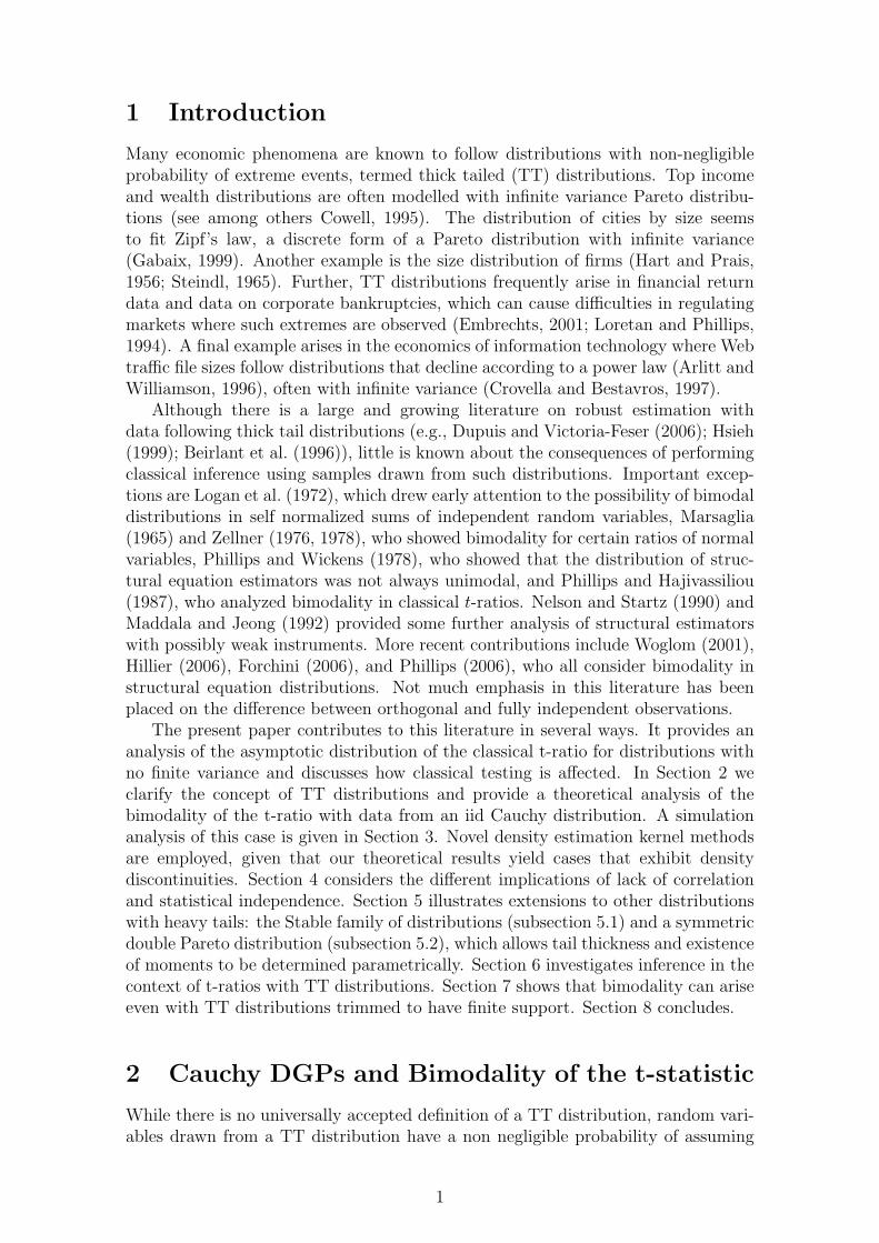
Bimodal t-ratios:

The Impact of Thick Tails on Inference

Carlo V. Fiorio1,Vassilis A. Hajivassiliou2

andPeter C.B. Phillips3

November 2009

Abstract

This paper studies the distribution of the classical t-ratio with data generatedfrom distributions with no finite moments and shows how classical testing is af-fected by bimodality. A key condition in generating bimodality is independenceof the observations in the underlying data generating process (DGP). The paperhighlights the strikingly different implications of lack of correlation versus statisti-cal independence in DGPs with infinite moments and shows how standard inferencecan be invalidated in such cases, thereby pointing to the need for adapting estima-tion and inference procedures to the special problems induced by thick-tailed (TT)distributions.

The paper presents theoretical results for the Cauchy case and develops a newdistribution termed the “double Pareto,” which allows the thickness of the tailsand the existence of moments to be determined parametrically. It also investigatesthe relative importance of tail thickness in case of finite moments by using TTdistributions truncated on a compact support, showing that bimodality can persisteven in such cases. Simulation results highlight the dangers of relying on naivetesting in the face of TT distributions. Novel density estimation kernel methodsare employed, given that our theoretical results yield cases that exhibit densitydiscontinuities.

Acknowledgements: The authors would like to thank the Coeditor and anony-mous referees for constructive comments and suggestions. The usual disclaimerapplies.

JEL codes: C12, C15, C46

1University of Milan and Econpubblica2London School of Economics and Financial Markets Group3Yale University, University of Auckland, Singapore Management University, and University of

York

1 Introduction

Many economic phenomena are known to follow distributions with non-negligibleprobability of extreme events, termed thick tailed (TT) distributions. Top incomeand wealth distributions are often modelled with infinite variance Pareto distribu-tions (see among others Cowell, 1995). The distribution of cities by size seemsto fit Zipf’s law, a discrete form of a Pareto distribution with infinite variance(Gabaix, 1999). Another example is the size distribution of firms (Hart and Prais,1956; Steindl, 1965). Further, TT distributions frequently arise in financial returndata and data on corporate bankruptcies, which can cause difficulties in regulatingmarkets where such extremes are observed (Embrechts, 2001; Loretan and Phillips,1994). A final example arises in the economics of information technology where Webtraffic file sizes follow distributions that decline according to a power law (Arlitt andWilliamson, 1996), often with infinite variance (Crovella and Bestavros, 1997).

Although there is a large and growing literature on robust estimation withdata following thick tail distributions (e.g., Dupuis and Victoria-Feser (2006); Hsieh(1999); Beirlant et al. (1996)), little is known about the consequences of performingclassical inference using samples drawn from such distributions. Important excep-tions are Logan et al. (1972), which drew early attention to the possibility of bimodaldistributions in self normalized sums of independent random variables, Marsaglia(1965) and Zellner (1976, 1978), who showed bimodality for certain ratios of normalvariables, Phillips and Wickens (1978), who showed that the distribution of struc-tural equation estimators was not always unimodal, and Phillips and Hajivassiliou(1987), who analyzed bimodality in classical t-ratios. Nelson and Startz (1990) andMaddala and Jeong (1992) provided some further analysis of structural estimatorswith possibly weak instruments. More recent contributions include Woglom (2001),Hillier (2006), Forchini (2006), and Phillips (2006), who all consider bimodality instructural equation distributions. Not much emphasis in this literature has beenplaced on the difference between orthogonal and fully independent observations.

The present paper contributes to this literature in several ways. It provides ananalysis of the asymptotic distribution of the classical t-ratio for distributions withno finite variance and discusses how classical testing is affected. In Section 2 weclarify the concept of TT distributions and provide a theoretical analysis of thebimodality of the t-ratio with data from an iid Cauchy distribution. A simulationanalysis of this case is given in Section 3. Novel density estimation kernel methodsare employed, given that our theoretical results yield cases that exhibit densitydiscontinuities. Section 4 considers the different implications of lack of correlationand statistical independence. Section 5 illustrates extensions to other distributionswith heavy tails: the Stable family of distributions (subsection 5.1) and a symmetricdouble Pareto distribution (subsection 5.2), which allows tail thickness and existenceof moments to be determined parametrically. Section 6 investigates inference in thecontext of t-ratios with TT distributions. Section 7 shows that bimodality can ariseeven with TT distributions trimmed to have finite support. Section 8 concludes.

2 Cauchy DGPs and Bimodality of the t-statistic

While there is no universally accepted definition of a TT distribution, random vari-ables drawn from a TT distribution have a non negligible probability of assuming

1

very large values. Distribution functions with infinite first moments certainly be-long to the family of thick tail (TT) distributions. Different TT distributions havediffering degrees of thick-tailedness and, accordingly, quantitative indicators havebeen developed to evaluate the probability of extremal events, such as the extremalclaim index to assign weights to the tails and thus the probability of extremal events(Embrechts et al., 1999). A crude though widely used definition describes any distri-bution with infinite variance as a TT distribution. Other weaker definitions requirethe kurtosis coefficient to larger than 3 (leptokurtic) (Bryson, 1982).

In this paper we say that a distribution is thick-tailed (TT) if it belongs tothe class of distributions for which Pr(|X| > c) = c−α and α ≤ 1. The Cauchydistribution corresponds to the boundary case where α = 1. Such distributions aresometimes called very heavy tailed.

It is well known that ratios of random variables frequently give rise to bimodaldistributions. Perhaps the simplest example is the ratio R = a+x

b+ywhere x and y

are independent N(0, 1) variates and a and b are constants. The distribution of Rwas found by Fieller (1932) and its density may be represented in series form interms of a confluent hypergeometric function [see (Phillips, 1982)][equation (3.35)].It turns out, however, that the mathematical form of the density of R is not the mosthelpful instrument in analyzing or explaining the bimodality of the distribution thatoccurs for various combinations of the parameters (a, b). Instead, the joint normaldistribution of the numerator and denominator statistics, (a + x, b + y) providesthe most convenient and direct source of information about the bimodality. Aninteresting numerical analysis of situations where bimodality arises in this exampleis given by Marsaglia (1965), who shows that the density of R is unimodal or bimodalaccording to the region of the plane in which the mean (a, b) of the joint distributionlies. Thus, when (a, b) lies in the positive quadrant the distribution is bimodalwhenever a is large (essentially a > 2.257 ).

Similar examples arise with simple posterior densities in Bayesian analysis andcertain structural equation estimators in econometric models of simultaneous equa-tions. Zellner (1978) provides an interesting example of the former, involving theposterior density of the reciprocal of a mean with a diffuse prior. An importantexample of the latter is the simple indirect least squares estimator in just identifiedstructural equations as studied, for instance, by Bergstrom (1962) and recently byHillier (2006), Forchini (2006), and Phillips (2006).

The present paper shows that the phenomenon of bimodality can also occur withthe classical t-ratio test statistic for populations with undefined second moments.The case of primary interest to us in this paper is the standard Cauchy (0,1) withdensity

pdf(x) =1

π(1 + x2)(1)

When the t-ratio test statistic is constructed from a random sample of n draws fromthis population, the distribution is bimodal even in the limit as n →∞. This caseof a Cauchy (0,1) population is especially important because it highlights the effectsof statistical dependence in multivariate spherical populations. To explain why thisis so, suppose (X1, · · · , Xn) is multivariate Cauchy with density

pdf(x) =Γ(n+1

2

)π(n+1)/2(1 + x′x)(n+1)/2

(2)

2

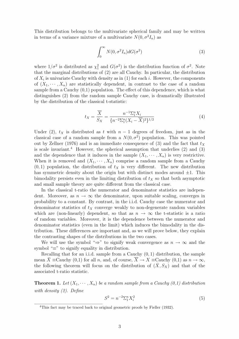
This distribution belongs to the multivariate spherical family and may be writtenin terms of a variance mixture of a multivariate N(0, σ2In) as∫ ∞

0

N(0, σ2In)dG(σ2) (3)

where 1/σ2 is distributed as χ21 and G(σ2) is the distribution function of σ2. Note

that the marginal distributions of (2) are all Cauchy. In particular, the distributionof Xi is univariate Cauchy with density as in (1) for each i. However, the componentsof (X1, · · · , Xn) are statistically dependent, in contrast to the case of a randomsample from a Cauchy (0,1) population. The effect of this dependence, which is whatdistinguishes (2) from the random sample Cauchy case, is dramatically illustratedby the distribution of the classical t-statistic:

tX =X

SX=

n−1Σn1Xi

{n−2Σn1 (Xi −X)2}1/2

(4)

Under (2), tX is distributed as t with n − 1 degrees of freedom, just as in theclassical case of a random sample from a N(0, σ2) population. This was pointedout by Zellner (1976) and is an immediate consequence of (3) and the fact that tXis scale invariant.4 However, the spherical assumption that underlies (2) and (3)and the dependence that it induces in the sample (X1, · · · , Xn) is very restrictive.When it is removed and (X1, · · · , Xn) comprise a random sample from a Cauchy(0, 1) population, the distribution of tX is very different. The new distributionhas symmetric density about the origin but with distinct modes around ±1. Thisbimodality persists even in the limiting distribution of tX so that both asymptoticand small sample theory are quite different from the classical case.

In the classical t-ratio the numerator and denominator statistics are indepen-dent. Moreover, as n → ∞ the denominator, upon suitable scaling, converges inprobability to a constant. By contrast, in the i.i.d. Cauchy case the numerator anddenominator statistics of tX converge weakly to non-degenerate random variableswhich are (non-linearly) dependent, so that as n → ∞ the t-statistic is a ratioof random variables. Moreover, it is the dependence between the numerator anddenominator statistics (even in the limit) which induces the bimodality in the dis-tribution. These differences are important and, as we will prove below, they explainthe contrasting shapes of the distributions in the two cases.

We will use the symbol “⇒” to signify weak convergence as n → ∞ and thesymbol “≡” to signify equality in distribution.

Recalling that for an i.i.d. sample from a Cauchy (0, 1) distribution, the samplemean X ≡Cauchy (0,1) for all n, and, of course, X → X ≡Cauchy (0,1) as n→∞,the following theorem will focus on the distribution of (X, SX) and that of theassociated t-ratio statistic.

Theorem 1. Let (X1, · · · , Xn) be a random sample from a Cauchy (0,1) distribution

with density (2). Define

S2 = n−2Σn1X

2i (5)

4This fact may be traced back to original geometric proofs by Fieller (1932).

3

t =X

S(6)

Then:

(a)

S2 ⇒ Y

where Y is a stable random variate with exponent α = 1/2 and characteristic func-

tion given by

cfY (v) = E(eivY ) = exp

{− 2

π1/2cos(π

4

)|v|1/2

[1− isgn(v)tan

(π4

)]}(7)

(b)

(X,S2)⇒ (X, Y )

where (X, Y ) are jointly stable variates with characteristic function given

cfX,Y = exp

{−2π−1/2(−iv)−1/2

1F1

(−1

2,1

2;u2/4iv

)}(8)

where 1F1 denotes the confluent hypergeometric function. An equivalent form is

cfX,Y (u, v) = exp{−|u| − π−1/2e−iu

2/4vΨ(3/2, 3/2; iu2/4v)}

(9)

where Ψ denotes the confluent hypergeometric function of the second kind.

(c)

S2 − S2X = Op(n

−1) (10)

t− tX = Op(n−1) (11)

(d) The probability density of the t-ratio (6) is bimodal, with infinite poles at ±1.

Proof. See Appendix A.

Theorem 1 establishes the joint distribution of (X, S2) and shows that the dis-tributions of t and tX , and of S and SX are respectively asymptotically equivalent.5

5For the definition of the hypergeometric functions that appear in (8) and (9) see Lebedev(1972, Ch. 9). Note that when u = 0 (8) reduces to

exp{−2π−1/2(−iv)1/2

}(12)

We now write −iv in polar form as

−iv = |v|e−isgn(v)π/2

so that(−iv)1/2 = |v|1/2e−isgn(v)π/4 = |v|1/2cos(π/4) (1− isgn(v)tan(π/4)) (13)

from which it is apparent that (8) reduces to the marginal characteristic function of the stable

4

Note that X2i has density

pdf(y) =1

πy1/2(1 + y), y > 0 (14)

In fact, X2i belongs to the domain of attraction of a stable law with exponent

α = 1/2. To see this, we need only verify (Feller, 1971, p. 313) that if F (y) is thedistribution function of X2

i then

1− F (y) + F (−y) ∼ 2/πy1/2, y →∞

which is immediate from (14); and that the tails are well balanced. Here we have:

1− F (y)

1− F (y) + F (−y)→ 1,

F (−y)

1− F (y) + F (−y)→ 0

Note also that the characteristic function of the limiting variate Y given by (7)belongs to the general stable family, whose characteristic function (see Ibragimovand Linnik (1971)][p.43]) has the following form:

ϕ(v) = exp{iγv − c|v|α

[1− iβsgn(v)tan

(πα2

)]}(15)

In the case of (7) the exponent parameter α = 1/2, the location parameter γ = 0, thescale parameter c = 2π−1/2cos(π/4) and the symmetry parameter β = 1. Part (a)of Theorem 1 shows that the denominator of the t ratio (6) is the square root ofa stable random variate in the limit as n → ∞. This is to be contrasted with theclassical case where nS2

X →pσ2 = E(X2

i ) under general conditions.

Note that when n = 1, the numerator and denominator of t are identical upto sign. In this case we have t = ±1 and the distribution assigns probability massof 1/2 at +1 and -1. When n > 1 the numerator and denominator statistics of tcontinue to be statistically dependent. This dependence persists as n→∞.

Figures 1a-d show Monte Carlo estimates (by smoothed kernel methods) of thejoint probability surface of (X,S2) for various values of n. As is apparent from thepictures the density involves a long curving ridge that follows roughly a parabolicshape in the (X,S2) plane. OLS estimates of the ridge in the joint pdf stabilizequickly as a function of n and confirm the dependence between X and S2 for theCauchy DGP.

Further note that the ridge in the joint density is symmetric about the S2 axis.The ridge is associated with clusters of probability mass for various values of S2 oneither side of the S2 axis and equidistant from it. These clusters of mass along theridge produce a clear bimodality in the conditional distribution of X given S2 forall moderate to large S2 . For small S2 the probability mass is concentrated in thevicinity of the origin in view of the dependence between X and S2. The clustersof probability mass along the ridge in the (X, S2) plane are also responsible for thebimodality in the distribution of certain ratios of the statistics (X,S2) such as the

variate Y given earlier in (7). When v = 0 the representation (9) reduces immediately to themarginal characteristic function, exp(−|u|), of the Cauchy variate X . In the general case the jointcharacteristic function cfXY (u, v) does not factorize and X and Y are dependent stable variates.

5

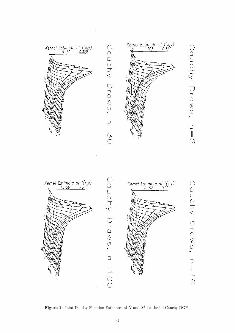
Figure 1: Joint Density Function Estimates of X and S2 for the iid Cauchy DGPs

6

t ratio statistics t = X/S and tX = X/SX . These distributions are investigated bysimulation in the following section.

3 Simulation Evidence for the Cauchy Case

The empirical densities reported here were obtained as follows: For a given valueof n, m = 10, 000 random samples of size n were drawn from the standard Cauchydistribution with density given by (1) and corresponding cumulative distributionfunction

F (x) =1

πarctan(x) +

1

2,−∞ < x <∞. (16)

Since (16) has a closed form inverse, the probability integral transform method wasused to generate the draws.

To estimate the probability density functions, conventional kernel methods, e.g.,Tapia and Thompson (1978), would not provide consistent estimates of the true den-sity in a neighbourhood of ±1 in view of the infinite singularities (poles) there. Anextensive literature considers how to correct the so-called boundary effect, althoughthere is no single dominating solution that is appropriate for all shapes of density.6

The method adopted here follows Zhang et al. (1999), which is a combination ofmethods of pseudodata, transformation and reflection, is nonnegative anywhere,and performs well compared to the existing methods for almost all shapes of densi-ties and especially for densities with substantial mass near the boundary. For theunivariate densities (Figures 2, 4, and 5) a bandwidth of h = 0.2 was used, while forthe bivariate densities in Figure 1, we employed equal bandwidths hx = hy = 0.2.

We investigated the sampling behavior of the t-ratio statistics t and tX , bycombining four kernel densities, two estimating the density on the left of ±1 andtwo estimating the density on the right of ±1 using the fact that for x > 1 + h,x < −1 − h and −1 + h < x < 1 − h the densities estimated with and withoutboundary correction coincide (Zhang et al. (1999, p. 1234)). These are shown inFigure 2. Note that the bimodality is quite striking and persists for all sample sizes.

4 Lack of Correlation versus Independence

Data from an n dimensional spherical population with finite second moments havezero correlation, but are independent only when normally distributed. The standardmultivariate Cauchy (with density given by (2)) has no finite integer moments but itsspherical characteristic may be interpreted as the natural analogue of uncorrelatedcomponents in multivariate families with thicker tails. When there is only “lack ofcorrelation” as in the spherical Cauchy case, it is well known (e.g., (King, 1980)) thatthe distribution of inferential statistics such as the t-ratio reproduce the behaviorthat they have under independent normal draws. When there are independent drawsfrom a Cauchy population, the statistical behavior of the t-ratio is very different.

6For an introductory discussion of density estimation on bounded support, cf. Silverman (1986,p. 29). Methods to correct for the boundary problem include the reflection method (Cline and Hart,1991; Silverman, 1986), the boundary kernel method (Cheng et al., 1997; Jones, 1993; Zhang andKarunamuni, 1998), the transformation method (Marron and Ruppert, 1994) and the pseudodatamethod (Cowling and Hall, 1996).

7

−3 −2 −1 0 1 2 3

0.0

0.1

0.2

0.3

0.4

0.5

t−ratio

kern

el e

stim

ate

of f(

t)Cauchy

n=10n=100n=500n=10000

−3 −2 −1 0 1 2 3

0.0

0.1

0.2

0.3

0.4

0.5

tX−ratio

kern

el e

stim

ate

of f(

t)

n=10n=100n=500n=10000

(a) Density Function of the t-ratio

−3 −2 −1 0 1 2 3

0.0

0.1

0.2

0.3

0.4

0.5

t−ratio

kern

el e

stim

ate

of f(

t)

Cauchy

n=10n=100n=500n=10000

−3 −2 −1 0 1 2 3

0.0

0.1

0.2

0.3

0.4

0.5

tX−ratio

kern

el e

stim

ate

of f(

t)

n=10n=100n=500n=10000

(b) Density Function of the tx-ratio

Figure 2: Density Functions for iid Cauchy DGPs

8

Examples of this type highlight the statistical implications of the differences betweenlack of correlation and independence in nonnormal populations.

(a) Spherical (Dependent) (b) Independent (Nonspherical)

Figure 3: Bivariate Cauchy: Spherical (Dependent) vs. Independent (Nonspherical)

Figure 3 highlights these differences for the bivariate Cauchy case. The left panelplots the iso-pdf contours of the bivariate spherical Cauchy (with the two observa-tions being non-linearly dependent), while the right panel gives the contours forthe bivariate independent Cauchy case (where the distribution is non-spherical). Inview of the thick tails, we see the striking divergence between sphericality and sta-tistical independence: whereas for normal Gaussian distribution, sphericality (=un-correlatedness) and full statistical independence coincide, we confirm that for non-Gaussianity, sphericality is neither necessary nor sufficient for independence.7

These results confirm the findings of Hajivassiliou (2008), who emphasized thatwhen data are generated from distributions with thick tails, independence and zerocorrelation are very different properties and can have startlingly different outcomes.By construction, the random variables in the numerator of the t-ratio, X, is linearlyorthogonal to the S2

X variable in the square root of the denominator. Under Gaus-sianity, this orthogonality implies full statistical independence between numeratorand denominator. But in the case of data drawn from the Cauchy distribution,statistical independence of the numerator and denominator of the t-ratio rests cru-cially on whether or not the underlying data are independently drawn: if they aregenerated from a multivariate spherical Cauchy (with a diagonal scale matrix) andhence they are non-linearly dependent, then the numerator and denominator in factbecome independent and the usual unimodal t-distribution obtains. If, on the otherhand, they are drawn fully independently from one another, then X and S2

X turn outto be dependent and hence the density of the t-ratio exhibits the striking bimodalitydocumented here.

7Figure 10 of the extended version of this paper, Fiorio et al. (2008) considers 6 representativesquares on the domain of the bivariate Cauchy distributions, and calculates various measures ofdeviation from independence for the spherical, dependent version.

9

5 Is the Cauchy DGP Necessary for Bimodality?

Our attention has concentrated on the sampling and asymptotic behavior of statis-tics based on a random sample from an underlying Cauchy (0,1) population. Thishas helped to achieve a sharp contrast between our results and those that are knownto apply with Cauchy (0,1) populations under the special type of dependence im-plied by spherical symmetry. However, many of the qualitative results given here,such as the bimodality of the t ratios, continue to apply for a much wider class ofunderlying populations. In this Section we show that the bimodality of the t-ratiopersists for other heavy-tailed distributions. Two cases are illustrated: (a) drawsfrom the Stable family of distributions and (b) draws from the “Double-Pareto”distribution.

5.1 Draws from the Stable Family of Distributions

Let (X1, · · · , Xn) denote a random sample from a symmetric stable population withcharacteristic function

cf(s) = e−|s|α

(17)

and exponent parameter α < 2 then the t-ratios t and tX have bimodal densitiessimilar in form to those shown in Figure 2 above for the special case α = 1. Togenerate random variates characterized by (17) a procedure described in Section 1of Kanter and Steiger (1974) was used. In our experiments we considered severalexamples of stable distributions for various values of a. We found that the bimodalityis accentuated for α < 1 and attenuated as α → 2. When α = 2, of course, thedistribution is classical t with n − 1 degrees of freedom. In a similar vein to theCauchy case, we found the ridge in the joint density to be most pronounced forα = 1/3 but withers as α rises to 5/3. For extended simulation results see Fiorioet al. (2008).

5.2 Draws from the Double-Pareto Distribution

Analogous to the double-exponential (see, Feller, 1971, p. 49), we define the doublePareto distribution as the convolution of two independent Pareto (type I) distributedrandom variables, X1−X2, whereX1 andX2 have density α1β

α11 x−α1−1 (x ≥ β1, α1 >

0, β1 > 0) and α2βα22 (x)−α2−1 (x ≥ β2, α2 > 0, β2 > 0), respectively.8 Its density is∫ ∞−∞

(α1βα11 )(α2β

α22 )(x2 + t)−α1−1(x2)−α2−1dx2

and its first two moments are:9

E(x) =α1β1(α2 − 1)− α2β2(α1 − 1)

(α1 − 1)(α2 − 1)with α1 > 1, α2 > 1

V (x) =α1β

21

α1 − 2− 2α1α2β1β2

(α1 − 1)(α2 − 1)+

α2β22

α2 − 2with α1 > 2, α2 > 2

8The name double Pareto was also used by Reed and Jorgensen (2003) for the distribution of arandom variable that is obtained as the ratio of two Pareto random variables and is only definedover a positive support.

9For derivations, see Appendix B of the extended version of this paper, Fiorio et al. (2008).

10

The results that follow were obtained via Monte Carlo simulations from randomsamples of dimension n using the method of inverted CDFs, i.e., a random sampleof dimension n is extracted from a unit rectangular variate, U(0, 1), and then it ismapped into the sample space using the inverse CDF. The number of replicationsm was 10,000. This study allows one to disentangle some differences about theasymptotic distribution of the t-ratio statistic when either one or both first twomoments do not exist.10

The Cauchy and the double Pareto distribution with α1 = α2 ≤ 1 are bothsymmetric and have infinite mean. For these distributions, as the sample size in-creases, the statistic tX converges towards a stable distribution which is symmetricand bimodal. The convergence is fairly rapid, even for samples as small as 10, andthe two modes are located at ±1. For the double Pareto distribution we find thatthe t-ratio distribution does depend on αi, i = 1, 2: the lower is αi, the higher is theconcentration around the two modes (Figure 4(a)).

We also examined the case 1 < α < 2 and found that the t-ratio, tX , is notalways clearly bimodally distributed. The more α departs from 1 the less evidentis the bimodality of the t-ratio density and the clearer the convergence towards astandard normal distribution (Figure 4(b)). We set β = 3 but these results applyfor any value of β > 0, since β is simply a threshold parameter that does not affectthe tX statistic behavior.11

If α1 6= α2 it suffices to have either α1 ≤ 1 or α2 ≤ 1 for the double Pareto tohave infinite mean. However, in this case the t-ratio distribution does not have abimodal density, nor is it stable (see Figure 6 of the extended online version of thispaper, Fiorio et al. (2008)).

The regularity in the tX distribution for the symmetric double Pareto case leadsus to investigate the relationship between the first and second centered moments, inthe numerator and denominator of tX respectively. In Section 2 above, we showedthat if the distribution is Cauchy, the variance converges toward a unimodal dis-tribution with the mode lying in the interval (0, 1). However, if the distributionis double Pareto, the sample variance does not converge towards a stable distri-bution but becomes more dispersed as the sample size increases. This behaviourconfirms the surprising results obtained elsewhere (Ibragimov, 2004; Hajivassiliou,2008) concerning inference with thick-tailed (TT) distributions depending on thetail thickness parameter, α: for α = 1, the dispersion of the distribution of sampleaverages remains invariant to the sample size n, for α < 1 more observations actuallyhurt with the variance rising with n. Furthermore, the usual asset diversificationresult that spreading a given amount of wealth of a larger number of assets reducesthe variability of the portfolio no longer holds: with returns from a TT distributionthe variability may remain invariant to the number of assets composing the portfolioif α = 1, while portfolio variability actually rises with the number of assets if α < 1.In such cases, all eggs should be placed in the same basket. 12

10Using copulas, we could evaluate behaviour with correlated double Pareto draws. See Haji-vassiliou (2008) for a development of this idea. See also Ibragimov et al. (2003) for some generalresults.

11These findings can be proved theoretically along the lines of Appendix A: The theory behindthe Double-Pareto Figures 4(a)-4(b) corresponds to the Logan et al. (1972) case of p = 2 andProb(t < −q) ∼ rq−α = Prob(t > q) ∼ `q−α with r = `. When 0 < α < 1 as in (4(a)), the densityof tX has infinite singularities at ±1, while for 1 < α < 2 as in (4(b)) the density is continuousthroughout with modes at ±1.

12For specific analysis of the distribution of the variance of double Pareto distributions with

11

−3 −2 −1 0 1 2 3

0.0

0.1

0.2

0.3

0.4

0.5

tX−ratio

ke

rne

l e

stim

ate

of f(

t)

Double−Pareto, a1=.5, b1=3, a2=.5, b2=3

n=10n=100n=500n=10000

−3 −2 −1 0 1 2 30

.00

.10

.20

.30

.40

.5

tX−ratio

ke

rne

l e

stim

ate

of f(

t)

Double−Pareto, a1=.9, b1=3, a2=.9, b2=3

n=10n=100n=500n=10000

(a) t-ratio of infinite-first-moment double Pareto distributions (α < 1)

−3 −2 −1 0 1 2 3

0.0

0.1

0.2

0.3

0.4

0.5

tX−ratio

ke

rne

l e

stim

ate

of

f(t)

Double−Pareto, a1=1.1, b1=3, a2=1.1, b2=3

n=10n=100n=500n=10000

−3 −2 −1 0 1 2 3

0.0

0.1

0.2

0.3

0.4

0.5

tX−ratio

ke

rne

l e

stim

ate

of

f(t)

Double−Pareto, a1=1.8, b1=3, a2=1.8, b2=3

n=10n=100n=500n=10000

(b) t-ratio of finite-first-moment double Pareto distributions (1 < α ≤ 2)

Figure 4: t-ratios for Double Pareto Distributions

12

6 Rejection Probability Errors of t-ratios

The preceding results are relevant for hypothesis testing in regressions with errorsthat are independent and identically distributed from a TT distribution. They arealso relevant for testing the hypothesis of difference in means or other statistics oftwo samples when either or both come from a TT distribution.

How serious are the mistakes in such cases if the critical values of a N(0, 1)distribution are used in classical t-ratio testing? The issue is well illustrated usingthe p−value discrepancy plot (Davidson and MacKinnon, 1998).

Let us now summarize results, which are extensively described in Fiorio andHajivassiliou (2006). Assume that we have a random sample from a double Paretodistribution with 1 < α ≤ 2 and we run a test H0 : µ = µ0 against the alternativeHA : µ 6= µ0, where µ is the true mean and µ0 some value on the real line. Thesample mean is used to estimate µ. Performing such a test using the standard normalrather than the correct distribution causes the null hypothesis to be under-rejectedby quite a small amount, not larger than 5% for tests of size 5%, and even less fortests of size 1% or 10%. This conclusion would often lead us to ignore the caveat ofhaving a systematic error in rejection probability (ERP) using the standard normalfor testing two-sided hypothesis with a symmetric double Pareto distribution with1 < α ≤ 2. However, three important points should be noted.

The first is that the policy of ignoring the true nature of the t-ratio distributionunder this particular DGP may be an acceptable policy if the size of the test issmaller than 10%. If the test has a larger size - for instance 40% - the ERP canbe larger than 10 and is obviously more difficult to tolerate.13 Second, if the non-symmetric double Pareto distribution is considered, then the t-ratio statistic is noteven stable. Finally, although the “ignore” policy leads to minor errors (below ±5%)for one sided tests in the case of the double Pareto distribution, the ERP might bemuch larger for other TT processes.

7 Bimodality without Infinite Moments?

In order to investigate the relative importance of tail thickness and non-existence ofmoments, we consider a distribution truncated on a compact support, characterizedas follows:

Z =

{X iff |X| < cNA otherwise

(18)

where X is a standard Cauchy(0,1). The cutoff parameter c is a positive finite realnumber. Since the support of this distribution is by construction finite and compact,the moments of the r.v. Z are all finite.

The first trimmed distribution truncated on a compact support as in (18) thatwe consider is the Cauchy X ∼ Cauchy(0, 1), while the second is the double Pareto

infinite mean, and of the relationship between the sample mean and variance in this case, theinterested reader is referred to the extended online version of this paper, Fiorio et al. (2008).

13Although tests of size larger than 10% are rather unusual in economics it is much less so inother disciplines, such as physics, where the main point is often to maximize the power of thetest, rather than to minimize its size. Also in physics and other related sciences, it is common toconsider the “probable error” of a test procedure, which corresponds to a significance level of 50%.In such cases it is common to find confidence intervals with about 60% coverage probability (seefor instance Karlen, 2002).

13

law introduced introduced in subsection 5.2.By considering truncated versions of distributions whose untruncated counter-

parts do not have finite moments, we can control the relative importance of the tailswhile working with distributions with all moments finite. In the simulations below,we consider the following truncation points:

Truncated Cauchyc 500 1,000 3,000 5,000prob(cutoff tails) 0.0012 0.0006 0.0002 0.0001

Truncated Double Paretoc 5,000 100,000 250,000 500,000prob(cutoff tails), α = 0.5 0.049 0.011 0.0069 0.0048

The higher the absolute value of c is, the less attenuated the impact of tailbehaviour will be. In contrast, low absolute values of c imply cutting out most ofthe (thick) tails of the distribution.

The general conclusion is that the bimodality can appear also when momentsare finite and the sample size is finite, but reasonably large for many empiricalapplications. Our results with N = 500 show that the source of the bimodality isthe rate of tail behaviour and not unboundedness of support or non-existence ofmoments (Figure 5), the non-normal behavior being more evident the larger thetruncation point c.

The heuristic explanation for these results is that any large draw in a finite samplefrom the underlying TT distribution will tend to dominate both the numerator anddenominator of a t ratio statistic, even if the DGP distribution has bounded support.Especially when there is a single extremely large draw that dominates all others, thenthe t will be approximately ±1, therefore leading to a distribution that has modalactivity in the neighbourhood of these two points. Clearly, it is not necessary for thedistribution to have infinite moments or unbounded support for this phenomenonto occur.

8 Conclusions

This paper has investigated issues of inference from data based on independentdraws from TT distributions. When the distribution is TT with infinite moments,the standard t-ratio formed from a random sample does not converge to a standardnormal distribution and the limit distribution is bimodal. Conventional inferenceis invalidated in such cases and errors in the rejection probability in testing can beserious. Bimodality in the finite sample distribution of the t-ratio arises even incases of trimmed TT distributions, showing that non-existence of moments is notnecessary for the phenomenon to occur.

14

−3 −2 −1 0 1 2 3

−0

.10

.00

.10

.20

.30

.40

.5

tX−ratio

ke

rne

l e

stim

ate

of f(

t)

Truncated Cauchy, n=500, symmetric around zero, trimming points (c)

|c|=6x10^4,Pr(|x|>|c|)=.00001|c|=6x10^3,Pr(|x|>|c|)=.0001

|c|=6x10^2,Pr(|x|>|c|)=.001|c|=6x10, Pr(|x|>|c|)=.01

−3 −2 −1 0 1 2 3

−0

.10

.00

.10

.20

.30

.40

.5

tX−ratio

ke

rne

l e

stim

ate

of f(

t)

Truncated double−Pareto, a1=a2=.5, b1=b2=3, n=500. Symm. at zero.

|c|=30x10^8,Pr(|x|>|c|)=.00001|c|=40x10^6,Pr(|x|>|c|)=.0001

|c|=45x10^4,Pr(|x|>|c|)=.001|c|=50x10^2,Pr(|x|>|c|)=.01

(a) Truncated Cauchy, n = 500.

−3 −2 −1 0 1 2 3

−0

.10

.00

.10

.20

.30

.40

.5

tX−ratio

ke

rne

l e

stim

ate

of

f(t)

Truncated Cauchy, n=500, symmetric around zero, trimming points (c)

|c|=6x10^4,Pr(|x|>|c|)=.00001|c|=6x10^3,Pr(|x|>|c|)=.0001

|c|=6x10^2,Pr(|x|>|c|)=.001|c|=6x10, Pr(|x|>|c|)=.01

−3 −2 −1 0 1 2 3

−0

.10

.00

.10

.20

.30

.40

.5

tX−ratio

ke

rne

l e

stim

ate

of

f(t)

Truncated double−Pareto, a1=a2=.5, b1=b2=3, n=500. Symm. at zero.

|c|=30x10^8,Pr(|x|>|c|)=.00001|c|=40x10^6,Pr(|x|>|c|)=.0001

|c|=45x10^4,Pr(|x|>|c|)=.001|c|=50x10^2,Pr(|x|>|c|)=.01

(b) Truncated Double Pareto, a1 = a2 = .5, b1 = b2 = 3, n = 500.

Figure 5: t-ratio of Cauchy and double Pareto on compact support. Symmetricaround zero. Trimming Points (c)

15

9 Appendix A: Proof of Theorem 1

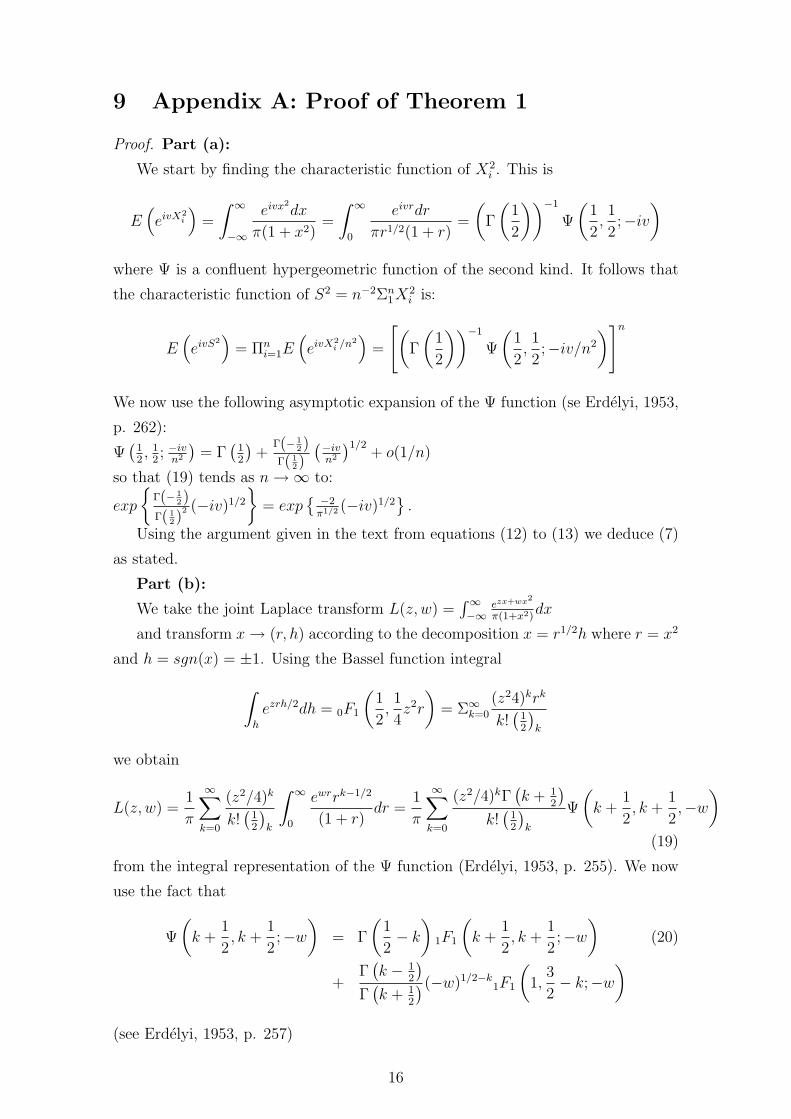
Proof. Part (a):

We start by finding the characteristic function of X2i . This is

E(eivX

2i

)=

∫ ∞−∞

eivx2dx

π(1 + x2)=

∫ ∞0

eivrdr

πr1/2(1 + r)=

(Γ

(1

2

))−1

Ψ

(1

2,1

2;−iv

)where Ψ is a confluent hypergeometric function of the second kind. It follows that

the characteristic function of S2 = n−2Σn1X

2i is:

E(eivS

2)

= Πni=1E

(eivX

2i /n

2)

=

[(Γ

(1

2

))−1

Ψ

(1

2,1

2;−iv/n2

)]n

We now use the following asymptotic expansion of the Ψ function (se Erdelyi, 1953,

p. 262):

Ψ(

12, 1

2; −ivn2

)= Γ

(12

)+

Γ(− 12)

Γ( 12)

(−ivn2

)1/2+ o(1/n)

so that (19) tends as n→∞ to:

exp

{Γ(− 1

2)Γ( 1

2)2 (−iv)1/2

}= exp

{ −2π1/2 (−iv)1/2

}.

Using the argument given in the text from equations (12) to (13) we deduce (7)

as stated.

Part (b):

We take the joint Laplace transform L(z, w) =∫∞−∞

ezx+wx2

π(1+x2)dx

and transform x→ (r, h) according to the decomposition x = r1/2h where r = x2

and h = sgn(x) = ±1. Using the Bassel function integral∫h

ezrh/2dh = 0F1

(1

2,1

4z2r

)= Σ∞k=0

(z24)krk

k!(

12

)k

we obtain

L(z, w) =1

π

∞∑k=0

(z2/4)k

k!(

12

)k

∫ ∞0

ewrrk−1/2

(1 + r)dr =

1

π

∞∑k=0

(z2/4)kΓ(k + 1

2

)k!(

12

)k

Ψ

(k +

1

2, k +

1

2,−w

)(19)

from the integral representation of the Ψ function (Erdelyi, 1953, p. 255). We now

use the fact that

Ψ

(k +

1

2, k +

1

2;−w

)= Γ

(1

2− k)

1F1

(k +

1

2, k +

1

2;−w

)(20)

+Γ(k − 1

2

)Γ(k + 1

2

)(−w)1/2−k1F1

(1,

3

2− k;−w

)(see Erdelyi, 1953, p. 257)

16

Γ(

12− k)

= π

(−1k)Γ(k+ 12)

and 1F1

(k + 1

2, k + 1

2;−w

)= e−w

Combining (19) and (20) we have:

L(z, w) =∞∑k=0

(−z2/4)k

k!(

12

)k

e−w (21)

+1

π

∞∑k=0

(z2/4)kΓ(k − 1

2

)k!(

12

)k

(−w)1/2−k1F1

(1,

3

2− k;−w

)

Let z = iuT

, w = ivT 2

It follows from (21) that

L(iuT, ivT 2

)= 1 +

(Γ(− 1

2)π

∑∞k=0

(− 12)k(u/4iv)k

k!( 12)k

)(−ivT 2

)1/2+ o

(1T

)and thus[L(iuT, ivT 2

)]T → exp

{Γ(− 1

2)π 1F1

(−1

2, 1

2; u

2

4iv

)(−iv)1/2

}Since cfX,S2(u, v) =

[L(iuT, ivT 2

)]Tand Γ

(−1

2

)= −2π1/2,

we deduce that

cfX,Y (u, v) = exp

{− 2

π1/2 1F1

(−1

2,1

2;u2

4iv

)(−iv)(1/2)

}(22)

as required for (8).

The second representation in this part of the Theorem is obtained by noting that

a−1xa1F1(a, a+ 1;−x) = Γ(a)− e−xΨ(1− a, 1− a, x)

(Erdelyi, 1953, p. 266). Using this result we find(−1

2

)−1

(−iv)1/21F1

(−1

2,1

2;u2

4iv

)=

1

2|u|{

Γ

(−1

2

)− eu2/4ivΨ

(3

2,3

2;−u2

4iv

)}.

(23)

Using (23) in (22) we obtain (9) as stated.

Part (c):

To prove equations (10) and (11), note that

S2X = S2 − n−1X

2= S2 + Op(n

−1) since X ⇒ Cauchy (0,1). Similarly, tX =

X [S2 +Op(n−1)]

−1/2= t+Op(n−1) as required.

Part (d):

To prove that the density of the t-ratio has singularities with infinite poles at

±1, it suffices to note that in the notation of Logan et al. (1972), the case of the

t-ratio (6) based on i.i.d. Cauchy draws corresponds to their parameters: p = 2,

α = 1, and r/l = 1. Then their equations (5.1) and (5.2) and Lemmas A and B

guarantee the result.

17

References

Arlitt, M. F. and Williamson, C. L. (1996). Web server workload characterization:The search for invariants. In Measurement and Modeling of Computer Systems,pages 126–137.

Beirlant, J., Vynckier, P., and Teugels, J. L. (1996). Tail Index Estimation, ParetoQuantile Plots, and Regression Diagnostics. Journal of the American StatisticalAssociation, 91(436):1659–1667.

Bergstrom, A. (1962). The exact sampling distributions of least squares and maxi-mum likelihood estimators of the marginal propensity to consume. Econometrica,30:480–490.

Bryson, M. (1982). Heavy-tailed distributions. In Kotz, N. and Read, S., editors,Encyclopedia of Statistical Sciences, volume 3, New York.

Cheng, M., Fan, J., and Marron, J. (1997). On automatic boundary corrections.The Annals of Statistics, 25:1691–1708.

Cline, D. and Hart, J. (1991). Kernel estimation of densities of discontinoususderivatives. Statistics, 22:69–84.

Cowell, F. A. (1995). Measuring Inequality. Harvester Wheatsheaf, Hemel Hemp-stead, second edition.

Cowling, A. and Hall, P. (1996). On pseudodata methods for removing boundaryeffects in kernel density estimation. Journal of the Royal Statistical Society, Ser.B, 551–563:58.

Crovella, M. and Bestavros, A. (1997). Self-Similarity in World Wide Web Traf-fic: Evidence and Possible Causes. IEEE/ACM Transactions on Networking,5(6):835–846.

Davidson, R. and MacKinnon, J. (1998). Graphical Methods for Investigating theSize and Power of Hypothesis Tests. The Mancester School, 66(1):1–26.

Dupuis, D. J. and Victoria-Feser, M. P. (2006). A Robust Prediction Error Criterionfor Pareto Modeling of Upper Tails. Canadian Journal of Statistics, 34:639–658.

Embrechts, P. (2001). Extremes in economics and the economics of extremes. paperpresented at SemStat meeting on Extreme Value Theory and Applications.

Embrechts, P., Klupperlberg, C., and Mikosch, T. (1999). Modelling Extremal Eventsfor Insurance and Finance. Springer Verlag, Berlin.

Erdelyi, A. (1953). Higher Trancendental Functions, Vol.1. McGraw-Hill, New York.

Feller, W. (1971). An Introduction to Probability Theory and its Applications, volumeVol.II. Wiley Press, New York, second edition.

Fieller, E. (1932). The distribution of the index in a noraml bivariate population.Biometrika, (24):428–440.

18

Fiorio, C., Hajivassiliou, V., and Phillips, P. (2008). Bimodal t-ratios: The impact of thick tails on inference. Downloadable from:http://econ.lse.ac.uk/staff/vassilis/papers/.

Forchini, G. (2006). On the bimodality of the exact distribution of the tsls estimator.Econometric Theory, 22, No.5:932–946.

Gabaix, X. (1999). Zipf’s law for cities: an explanation. The Quarterly Journal ofEconomics, 114(3):739–767.

Hajivassiliou, V. (2008). Correlation versus statistical dependence and thick taildistributions: Some surprising results. LSE Department of Economics WorkingPaper.

Hart, P. E. and Prais, S. J. (1956). An analysis of business concentration. Journalof the Royal Statistical Society, A, 119:150–181.

Hillier, G. (2006). Yet more on the exact properties of iv estimators. EconometricTheory, 22, No.5:913 – 931.

Hsieh, P.-H. (1999). Robustness of Tail Index Estimation. Journal of Computationaland Graphical Statistics, 8(2):318–332.

Ibragimov, I. and Linnik, V. (1971). Independent and Stationary Sequences of Ran-dom Variables. Noordhorf, Groninger-Wolter.

Ibragimov, R. (2004). On the robustness of economic models to heavy-tailednessassumptions. Cowles Foundation Discussion Paper.

Ibragimov, R., de la Pena, V., and Sharkhmetov, S. (2003). Characterizations of jointdistributions, copulas, information, dependence and decoupling, with applicationsto econometrics. Cowles Foundation Discussion Paper.

Jones, M. (1993). Simple boundary correction for kernel density estimation. Statis-tics and Computing, 3:135–146.

Kanter, M. and Steiger, W. (1974). Regression and autoregression with infinitevariance. Advances in Applied Probability, 6:768–783.

Karlen, D. (2002). Credibility of Confidence Intervals. In Advanced Statistical Tech-niques in Particle Physics, Proceedings, pages 53–57. Grey College, Durham.

King, M. (1980). Robust tests for spherical symmetry and their application to leastsquares regression. Annals of Statistics, 8:1265–1271.

Lebedev, N. (1972). Special Functions and Their Applications. Prentice-Hall, En-glewood Cliffs.

Logan, B., Mallows, C., Rice, S., and Shepp, L. (1972). Limit distributions ofself-normalized sums. Annals of Probability, 1:788–809.

Loretan, M. and Phillips, P. C. B. (1994). Testing the covariance stationarity ofheavy-tailed time series. Journal of Empirical Finance, (1):211–248.

19

Maddala, G. and Jeong, J. (1992). On the exact small sample disttribution of theinstrumental variable estimator. Econometrica, 60:181–183.

Marron, J. and Ruppert, D. (1994). Transformations to reduce boundary bias inkernel density estimation. Journal of the Royal Statistical Society, Ser. B, 56:653–671.

Marsaglia, G. (1965). Ratios of normal variables and ratios of sums of uniformvariables. Journal of the American Statistical Association, 60:193–204.

Nelson, C. and Startz, R. (1990). Some further results on the exact small sampleproperties of the instrumental variables estimator. Econometrica, 58:967–976.

Phillips, P. (2006). A remark on bimodality and weak instrumentation in structuralequation estimation. Econometric Theory, 22, No.5:947–960.

Phillips, P. and Wickens, M. (1978). Exercises in Econometrics. Philip Allan,Oxford.

Phillips, P. C. B. (1982). Exact small sample theory in the simultaneous equationmodel. In Intrilligator, M. and Griliches, Z., editors, Handbook of Econometrics,Amsterdam. North-Holland.

Phillips, P. C. B. and Hajivassiliou, V. A. (1987). Bimodal t-ratios. Cowles Foun-dation Discussion Paper No.842.

Reed, W. J. and Jorgensen, M. (2003). The double pareto-lognormal distribution anew parametric model for size distributions. mimeo.

Silverman, B. (1986). Density Estimation for Statistics and Data Analysis. Chapmanand Hall, London.

Steindl, J. (1965). Random Processes and The Growth of Firms. Griffin, London.

Tapia, R. and Thompson, J. (1978). Non Parametric Probability Density Estimation.The Johns Hopkins University Press, Baltimore.

Woglom, G. (2001). More results on the exact small sample properties of the in-strumental variable estimator. Econometrica, 69:1381–1389.

Zellner, A. (1976). Bayesian and non-bayesian analysis of the regression model withmultivariate student-t error terms. Journal of the American Statistical Associa-tion, 71:400–405.

Zellner, A. (1978). Estimation of functions of population means and regressioncoefficients including structural coefficients: A minimum expected loss (melo)approach. Journal of Econometrics, 8:127–158.

Zhang, S. and Karunamuni, R. (1998). On kernel density estimation near endpoints.Journal of Statistical Planning and Inference, 70:301–316.

Zhang, S., Karunamuni, R., and Jones, M. (1999). An improved estimator of thedensity function at the boundary. Journal of the American Statistical Association,94:1231–1241.

20