B i m o d a l Hi s togram Transformat ion Based on M a x i m u m Likel ihood Parameter Es t imates in

Univar iate Gauss ian Mixtures

Nette Schultz and Jens Michael Carstensen

Department of Mathematical Modelling, Building 321 Technical University of Denmark, DK-2800 Lyngby, Denmark. *

Abstract. This paper presents a bimodal histogram transformation pro- cedure where conjugate gradient optimization is used for estimating max- imum likelihood parameters of uuivariate Gaussian mixtures. The paper only deals with bimodai distributions but extension to mtfltimodal dis- tributions is fairly straightforward. The transformation is suggested as a preprocessing step that provides a standardized input to e.g. a classifier. This approach is used for pixelwise classification in RGB-images of meat.

1 Introduct ion

A transformation of image d a t a dis t r ibut ions can be used in image en- hancement to enhance specific sub levels in the intensity range. It can also be used as preprocessing before classification or segmentation. Com- mon transformations t ransform the image d a t a to more or less predeter- mined distributions with fixed parameters . By using a histogram match with predetermined distributions the h is togram information is totally neglected. The bimodal his togram t ransformat ion described here does not remove all the histogram informat ion, and is therefore interesting as standardization algorithm for d a t a t ha t is bimodal by nature. We will describe the bimodal his togram tra_~formation, which estimates the pa- rameters for a bimodal da t a set using max imum likelihood estimation, and only changes some of the pa ramete r s to predetermined fixed val- ues. It could as well be a h is togram t ransformat ion with more than two Gaussian distributions. The method is used as a preprocessing step in a classification case study. The case s tudy is to classify mea t images pixel-wise into lean or fat, where the meat images are cross-sectional cuts from pork carcasses. The images are 8-bit rgb color. The light exposures vary from image to ira-

* We would like to thank Hans Henrik Thodberg from the Danish Meat Research Institute and professor Knut Conradsen, associated professor Bjarne Ersb¢ll and the rest of the Image Group at Department of Mathematical Modelling, DTU.

533

age. Thus without some kind of s tandard iza t ion of the da ta the pixel-wise classification of lean and fat will be deter iorated, because the light in- tensity ranges in the images used as trainlrtg set for the classifications model estimation are changing in relat ion to the rest of the da ta set. We therefore apply the bimodal h is togram t ransformat ion to each rgb band.

When the intensi ty-function of the change in light exposure is unknown, and too much change in the distr ibut ion of an image is undesirable, the bimodal histogram t rans format ion can be one approach to overcome the difficulties of light exposure changes.

2 Dealing with Varying Light Exposure Our approach is to assume tha t the image is a mixture of Gaussians. We est imate the pa ramete r s - averages, variances and weights - and only change a minimum of pa rame te r s necessary to get the desired standard- ization or enhancement . In this actual case s tudy we will only be dealing with bimodality, but it can easily be ex tended to a mix ture of a larger number of Gaussians. When a da ta set is classified by means of supervised models, a training set is necessary. The t raining set is used for est imating parameters in the model. A common problem in many applications is, that the da ta set distributions can vary for different incidents. This means that the training set used for model es t imat ion will be different from the new data set, and can cause a poor classification. For pixel classification in an image, the light intensities can change over the image or from one image to another over time, dependent of the environment and image acquisition applications. In the meat classifica- tion case study, the pixels' light intensities are varying from dark and under exposed to light and over exposed images. Fig. 1 shows two differ- ent examples of meat images. T h e image intensities are changing in the range from dark to over exposed. These unstable light conditions makes a classification on the raw images troublesome. One way to overcome this problem is by using features which are invari- ant in relation to the intensi ty changes. Features which are invariant to linear t ransformations are e.g. skewness, kurtosis and orthogonal trans- formations like canonical variables and principal components based on the correlation matr ix. The t ransformation is, however, of ten nonlinear. Another approach is to t ransform the raw d a t a to a more or less fixed histogram distribution. A gentle t ransformation where only some of the distribution parameters are fixed can therefore be suitable. This t ransformation can be an univariate color scale calibration for images wi th bimodal histograms, where only the averages have been changed.

534

3 M a x i m u m L i k e l i h o o d E s t i m a t i o n of Parameters for B i m o d a l D a t a Sets Assuming the da ta set is a mix ture of Gaussians, see e.g. [3] the param- eters can be es t imated and used in the histogram transformation. In the univariate case the likelihood and its derivatives can easily be derived, and conjugate gradient can be used for estimating the maximum likelihood parameters . The mult ivar ia te case induces difficulties with the derivatives. Approximations to m a x i m u m likelihood est imation like the EM algorithm in [2] could be u sed in the mult ivariate case.

Fig. 1. From top to bottom an over exposed and under exposed image of meat is shown.

535

In the meat image pixel classification application, the histogram is as- sumed to be a mixture of two Gaussian distributions. Therefore we will only be dealing with bimodality, bu t the results can easily be extended to mixtures of more than two Gaussian distributions. The likelihood is

L(p1 ,#2 ,0 . t , 0 .2 , a )=

N . I 1 t i - - l i t 2 exp(--7( ~ 1 )

i=.l V ~ ' " ~ *

1 1 , 1 , t i - - #2~2~ expt-Tt . , (1)

where N is the number of observations, and tl is the value of observation number i.

The log likelihood is

N

In L(p t , #2, 0.z, 0.2, a) = E ln(a - - i----I

1 1 , l t t i --/~1 ~2,~ ~ ' ~ 0.1 e x p ( - - 2 t ~ ) )

I ti -- P2 2 + ( 1 - c ~ ) 1 1 e x p ( - ~ ( ~ ) )) (2) v / ~ 0.2

Let the data set be the pixel values in an image. The number of obser- vations is the number of pixels in the image, and the pixel values are integers in the range [0; Maxval]. T h e n the log likelihood can be writ ten as

Maxval

In L(D1, D2,0.1,0.2, or) - - n l f * ( i , DI , it2,0"1,0.2, a 0 (3)

i=o

where ni is the number of pixels with pixel value i, and

f~t(i,/-~1,/~2,0.1,0"2,0~) --" In(o/ 1 I exp(-- 1, i -- , 1 , 2 , J

+ ( l - - a ) ~ e ~ t - - ~ t - - - ~ j )) (4)

We want to estimate the parameters ( m , ~2, 0.1,0"2, cO as

arg max in L ( m , .2,0. t , 0.2, a) . (5)

As we are dealing with parameters belonging to Gaussian distributions, we have the following constraints

536

,,'1 > o, (6)

~-= > o, (7)

and o _< a _< 1. (s)

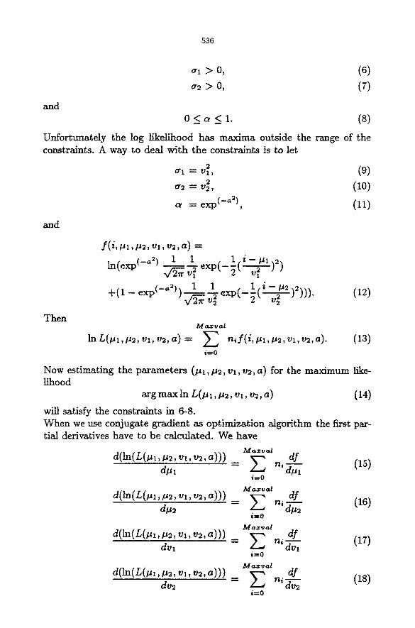
Unfortunately the log likelihood has maxima outside the range of the constraints. A way to deal wi th the constraints is to let

~', = ~,~, (9) ( lO) 0"2 ~ U 2

c~ = exp ( ), (11)

and

f ( i , pl,l~2, vl, v2,a) =

ln(exp(_a2) 1 1 . 1 . i -- ~t ~2~ V/~ v? exp(--~[ T ) )

1 1 1 i--/~2 2 +(1-- exP (-a2)) V/~v~ e x p ( - - 2 ( - - ~ 2 2 ) )))" (12)

Then

l n L ( m , p 2 , v l , v2, a) = M a : r v al

i=O

ni f ( i , pl,l.~2,Vl,v2,a). (13)

Now estimating the parameters (p l , p2, vl, v2, a) for the maximum like- lihood

arg max In L(pl , p2, vl, v2, a) (14)

will satisfy the constraints in 6-8. When we use conjugate gradient as opt imizat ion algorithm the first par- tial derivatives have to be calculated. We have

M a z r v a l d(ln( L ( m , p2 , vl, v2, a) ) )

d m

M a x v a l d(in( L ( m , ~ , v~ , v2, a) ) )

d~2 i=O

M a x v al d(ln( L ( m , I.t2, vl, v2, a) ) )

dr1

M a z : v a l d( in(L(m, .2 , vl, v2, a)))

de2 i----O

df dpl (15)

df (16) dtt2

df (17) dvl

~f (is) dr2

537

Where d/

dpl

M a x v a l d(ln( L(p, , p2 , v~, v2, a) ) ) df

da = E ni-~a" (19) i--O

e x p ( - a ~ ) . - ~ ( i -- U,) i ~ 2 e ~ p ( - - ~ ( ff ) )

(20)

df = ('2.1) dp2

(1 - - exp( - -a2) )~( i - - /~2) exp(--$(~ 'z~ ) ) 1 i -

exp(_~2) A~.I exp(_ ½(L~I )2) + (t _ exp(_~2)) ;_~_ 21 exp(-$(1 ~ , - ~ )~)

df = (22)

dvl 2 exp(_a2)_~ I , i - 2 ) ( ( ~ ) 1) e ~ ( - - ~ ( ~ ) ' - ~ -

exp(-~) ~ exp(-- 1 , - 2 _

df = (23) dr2

2(1 - - exp(--a2)) v--~2 exp(-- ~ . ( ~ ) 2 ) ((L~)i- 2 _ 1)

d f = (24) da

+

1 1 i - 2 1 1 " exp(-o~) ~ exp(- ~(~;-~) ) + (t - e~p(-°~))q e x p ( - ~ ( ' ' ~ ) )

A good starting value of the parameters can speed up the conjugate gradient algorithm, and make it less likely that the maximum likelihood estimation jumps into local maxima caused by noisy data. We obtain a starting guess by estimating the parameters on the one-dimensional mean filtered histogram. The averages are located as local maxima, the alfa by the local minimum in between the averages and the variances by the 5% and 95% fractiles. Conjugate gradient is used because it is relatively fast and the derivatives can be calculated.

538

The bimodal t ransformat ion procedure is as follows 1 Est imate a s tar t ing guess of the parameter values. 2 Calculate the derivatives of the parameters. 3 Est imate new paramete r values with conjugate gradient. 4 If the parameter-changes are below a pre-set limit, we may proceed,

otherwise go to s tep 2. 5 Transform the image histogram to a histogram with the predeter-

mined parameter values and the other estimated parameter values.

4 Case Study: Pixel-wise Classification of Meat Images

The Danish slaughter-houses est imate the carcass meat percent by us- hag measurements as total weight, different anatomical lengths and local meat and fat measurements from optical insertion probes. By use of vision, we can get alternative features, for estimation of the meat percentage, see e.g. [1]. The areas of lean and fat in a slice of meat are intuitively correlated with the meat percent. Therefore, after the carcass has been divided into front part, middle part and h a m as it is usual in a slaughter house, one image ha color rgb, has been taken of the cut between front and middle part, and a second image has been taken of the cut between middle part and ham. Fig. 1 shows an image of the front (top) and an image of the ham (bottom). Assuming that the background has been removed from the image (by use of deformable templates as described in [1]). Our aim on this step is to classify the meat into lean and fat pixel by pixel.

4 .1 T h e H i s t o g r a m T r a n s f o r m a t i o n

The data set consists of 572 images. 283 images of the front and 289 images of the ham. In [4] several different classification methods have been used and compared on a subset of the data set. In the comparison a neural network wi thout hidden layers worked fairly well. The input features to the network was the raw rgb bands, the local median filtered bands and local s t andard deviation filtered bands. Therefore we will use this classification method . A representative training set has been selected from 12 of the images for model estimation.

539

Because of the changes in fight exposure over images we apply a bimodal histogram transformation to the raw rgb bands before any feature ex- traction. Here the averages are changed to predetermined values.

. . . . . . . . . . . . . . . . . . . . . . . . . . . . . . . .;i:!,:. , ¸

Fig . 2. Each image consist of three bands of format byte.From top to bot tom the red, green and blue band is shown.

In Fig. 2 the red, green and blue band of an image from the front is shown. The corresponding histograms are shown in Fig. 3. The pLxel values are in the range 0-255. The histograms do not look very nice.

i

Fig . 3. Histograms in range 0-255 of the red, green and blue band from left to right.

540

They are very spiky, probably due to a preference with regard to the least significant bit. Fur thermore there is a clear difference between the green compared to the red and blue band recording method. Therefore a change in the sample space can be preferable.

Fig. 4. Histograms in range 0-128 of the red, green and blue band from left to right.

Fig. 5. Histograms in range 0-64 of the red, green and blue band from left to right.

In Fig. 4 and 5 the his tograms with sample ranges 0-128 and 0-64 are shown. The corresponding es t imated density, where the maximum like- lihood estimation of paramete rs is used, is also shown as an overlaid graph. The densities seem to fit the da ta set fairly well, though the data set is noisy and actllally could look like a mixture of three Gaussians. Because the lean can vary in darkness coursed by anatomical differences in the muscles, the lean class distr ibution could actually be a mixture of two normal distributions. But these differences are G~y visible in some of the images.

541

t, Fig. 6. Histograms in range 0-64 of the bimodal histogram transformed red, green and blue band from left to right.

Fig. 7. The red, green and blue band - top to bottom - after bimodal histogram trans- formation.

The result of a bimodal histogram t rans format ion is shown in Fig. 6 as histograms and 7 as images. We have used the histograms in the range 0- 64 in Fig. 5 and, as described in Section 3, t ransformed them by changing the mean values and keeping the variances and alpha. In this case the resulting image has become darker, and the classification between lean and fat will be improved.

542

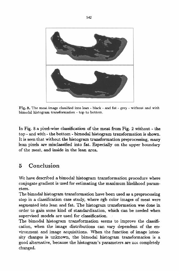
F i g . 8. T h e m e a t image classified in to lean - b lack - a n d fa t - grey - w i t h o u t a n d w i t h

b i m o d a l h i s t o g r a m t r a n s f o r m a t i o n - t o p to b o t t o m .

In Fig. 8 a pixel-wise classification of the meat from Fig. 2 without - the top - and with - the bottom - bimodal histogram transformation is shown. It is seen that without the histogram tran.*formation preprocessing, many lean pixels are misclassified into fat. Especially on the upper boundary of the meat, and inside in the lean area.

5 Conclusion

We have described a bimodal histogram transformation procedure where conjugate gradient is used for estimating the maximum likelihood param- eters. The bimodal histogram transformation have been used as a preprocessing step in a classification case study, where rgb color images of meat were segmented into lean and fat. The histogram transformation was done in order to gain some kind of standardization, which can be needed when supervised models are used for classification. The bimodal histogram transformation seems to improve the classifi- cation, when the image distributions can vary dependent of the en- vironment and image acquisitions. When the function of image inten- sity changes is unknown, the bimodal histogram transformation is a good alternative, because the histogram's parameters are ao~ completely changed.

543

References

1. N. Schultz. Segmentation and classification of biological objects. PhD thesis, Institute of Mathematical Modelling , Technical University of Denmark, Lyngby, 1995. 194 pp.

2. T. Taxt, N.L. Hjort, and L. Eikvil. Statistical classification using a linear mixture of two multinormal probability densities. Pattern Recognition Letters, 12(12):731-737, 1991.

3. D.M. Titterington, A.F.M. Smith, and U.E. Makov. Statistical anal- ysis of finite mixture distributions. J. Wiley & Sons, Great Britain, 1985. 243 pp.

4. C. Vind. A comparison of neural networks and statistical methods for classification. Master's thesis, Institute of Computer Science, Copen- hagen University and the Danish Meat Research Institute, University of Copenhagen, Denmark, 1994.