Embed Size (px)
Citation preview
Bimodal Chunking
Erik Kruus
Cezary Dubnicki
Cristian Ungureanu
Feb 29, 2010
Work done at NEC laboratories 1
Content defined chunking
Motivation, approach
Introduce bimodal algorithms, transition regions
Example algorithms
Results
Conclusions, Questions
Outline
2
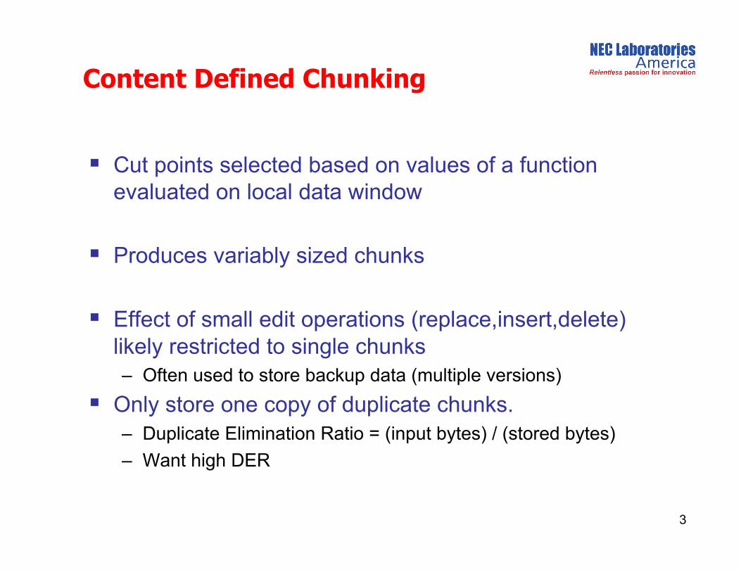
Cut points selected based on values of a function evaluated on local data window
Produces variably sized chunks
Effect of small edit operations (replace,insert,delete) likely restricted to single chunks – Often used to store backup data (multiple versions)
Only store one copy of duplicate chunks. – Duplicate Elimination Ratio = (input bytes) / (stored bytes)
– Want high DER
Content Defined Chunking
3

To get reproducible chunks, fix various parameters…
Function evaluated on local window – Choice not so important (typically a fast, rolling hash function)
Average chunk size – Depends on predicate used to select cut point
– Ex. “function of local data window has 10 LSBs zero” • Expect 1 match out of every 1024
Minimum chunk size, Maximum chunk size – Random chunk boundary selection geometric distribution of
chunk sizes. Too many small chunks!
… – Perhaps mechanism for reducing # of occurences of non-
content-defined cut points as a result of max chunk size
Baseline Chunking Parameters
4

?
Larger blocks help I/O performance
Larger blocks reduce metadata storage overhead – Large storage systems may have many bytes of metadata
associated with each chunk.
Motivation
5
Small block size:
High DER
Large Block size:
Low DER
Desire Large Blocks and High DER

So what can we do improve the chunking algorithm? – Use other easily-available information
In this work we investigate what can be done if a fast chunk existence query is available.
NECLA archive data set: 14 backups of the main filesystem used by lab’s researchers every day. Full backups done every other week totaled 1.1 TB. – Analyses done using smaller chunking summary of the full
dataset.
Approach
6

Bimodal Algorithms
unimodal chunking
Input data block boundaries
block size
64 KB
Uni-modal distribution
bimodal chunking
Input data block boundaries
block size
64 KB
Bimodal distribution
8 KB
block repository
block existence query yes/no

“Historical” intuitions
8
Intuitive model of file system backups 1. Long stretches of unseen data should be assumed to be
good candidates for appearing later on (i.e. at the next backup run). • Original data should have reasonable DER to begin with
• Long stretches of unseen data should be chunked with large average chunk size.
2. Inefficiency around “change regions” straddling boundaries between duplicate and unseen data can be minimized by using shorter chunks.
Inefficiency: short blocks can delineate the beginnings and ends of duplication regions more finely.
Change regions: existence queries give us a way to detect these transition regions
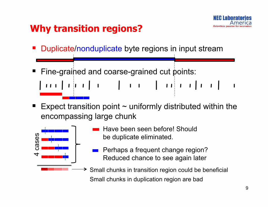
Duplicate/nonduplicate byte regions in input stream
Fine-grained and coarse-grained cut points:
Expect transition point ~ uniformly distributed within the encompassing large chunk
Why transition regions?
9
Have been seen before! Should be duplicate eliminated.
Perhaps a frequent change region? Reduced chance to see again later
Small chunks in transition region could be beneficial
Small chunks in duplication region are bad
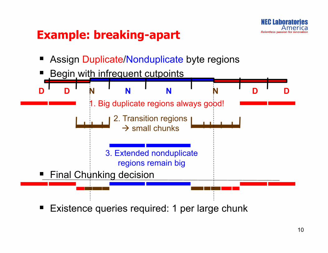
Assign Duplicate/Nonduplicate byte regions
Begin with infrequent cutpoints
Example: breaking-apart
10
D N N N N D D D
2. Transition regions small chunks
3. Extended nonduplicate regions remain big
1. Big duplicate regions always good!
Final Chunking decision
Existence queries required: 1 per large chunk
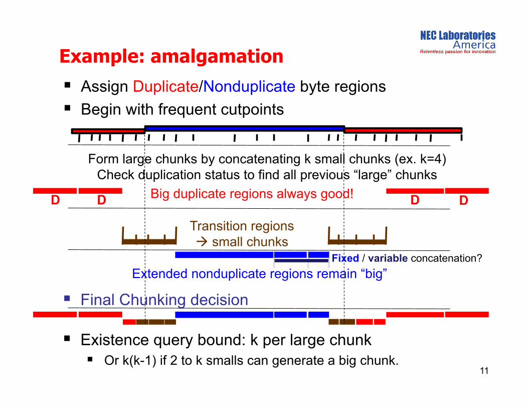
Assign Duplicate/Nonduplicate byte regions
Begin with frequent cutpoints
Form large chunks by concatenating k small chunks (ex. k=4) Check duplication status to find all previous “large” chunks
Example: amalgamation
11
Transition regions small chunks
Extended nonduplicate regions remain “big”
Big duplicate regions always good!
Final Chunking decision
D D D D
Fixed / variable concatenation?
Existence query bound: k per large chunk Or k(k-1) if 2 to k smalls can generate a big chunk.

Transition region subcases
12
Statistics of small chunks for some frequent subcases of fixed-size (8) amalgamation: Baseline chunkers with average
chunk size from 4k to 24k.
Extend to 32 chunks, see “bulk” 8k small chunk recurrence prob. tailing off to ~65%
1.1 Tb
Will I ever see you again?
Ask an oracle – Using transition regions to guide small chunk output
decisions gave future hit rates that were higher than “bulk” expectation

Based on full NECLA data set, how good could it get?
A simple, empirical limit
13
Concatenate all chunks that always occur together
x x
x x
Whenever a stored item has unique successor, merge!
For uncompressed storage, DER is unaffected
Began with 512-byte and 8k baseline chunkings of the full dataset (2 expts)
Result: almost 10x larger average block size
Algorithm not practical Uses post-processing
Computationally very expensive
10x
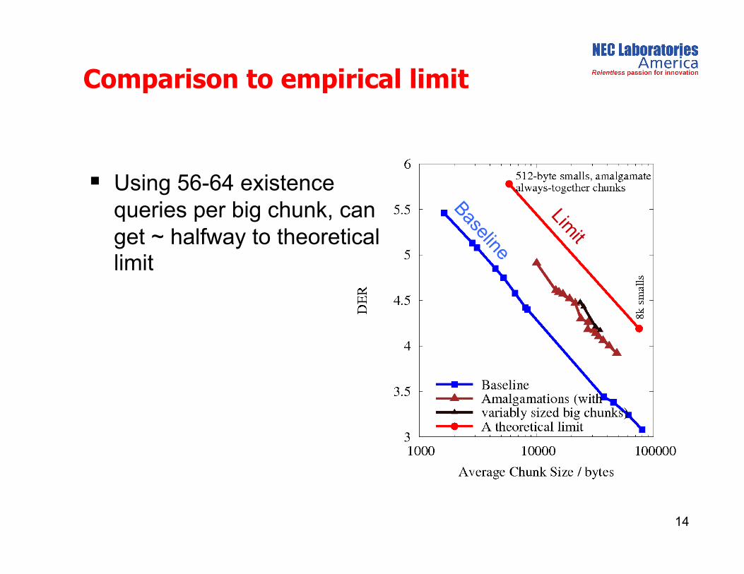
Comparison to empirical limit
14
Using 56-64 existence queries per big chunk, can get ~ halfway to theoretical limit
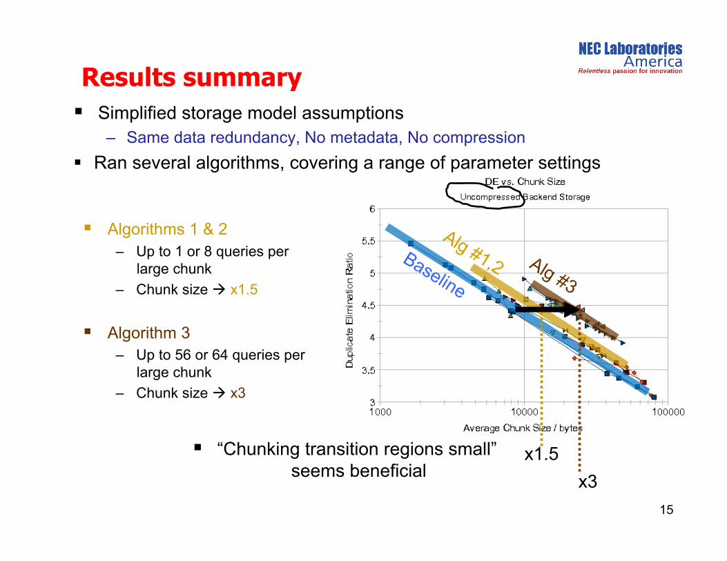
Results summary
15
x3
x1.5
Simplified storage model assumptions – Same data redundancy, No metadata, No compression
Ran several algorithms, covering a range of parameter settings
Algorithms 1 & 2
– Up to 1 or 8 queries per large chunk
– Chunk size x1.5
Algorithm 3 – Up to 56 or 64 queries per
large chunk
– Chunk size x3
“Chunking transition regions small” seems beneficial
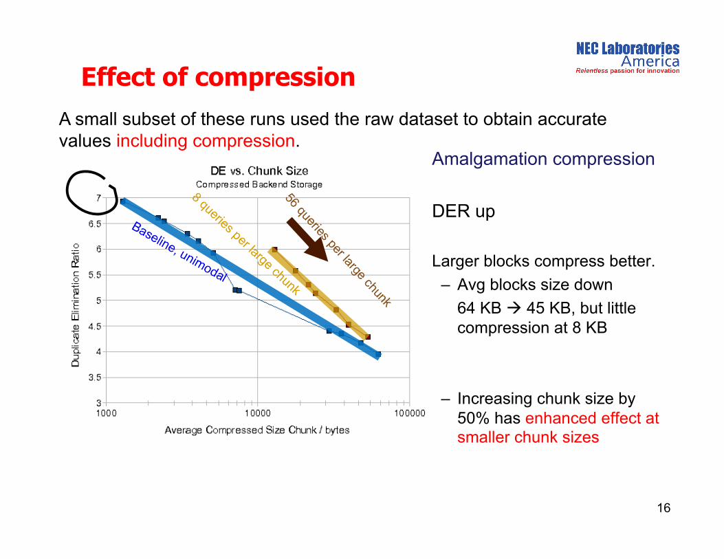
Effect of compression
16
A small subset of these runs used the raw dataset to obtain accurate values including compression.
Amalgamation compression
DER up
Larger blocks compress better.
– Avg blocks size down
64 KB 45 KB, but little compression at 8 KB
– Increasing chunk size by 50% has enhanced effect at smaller chunk sizes
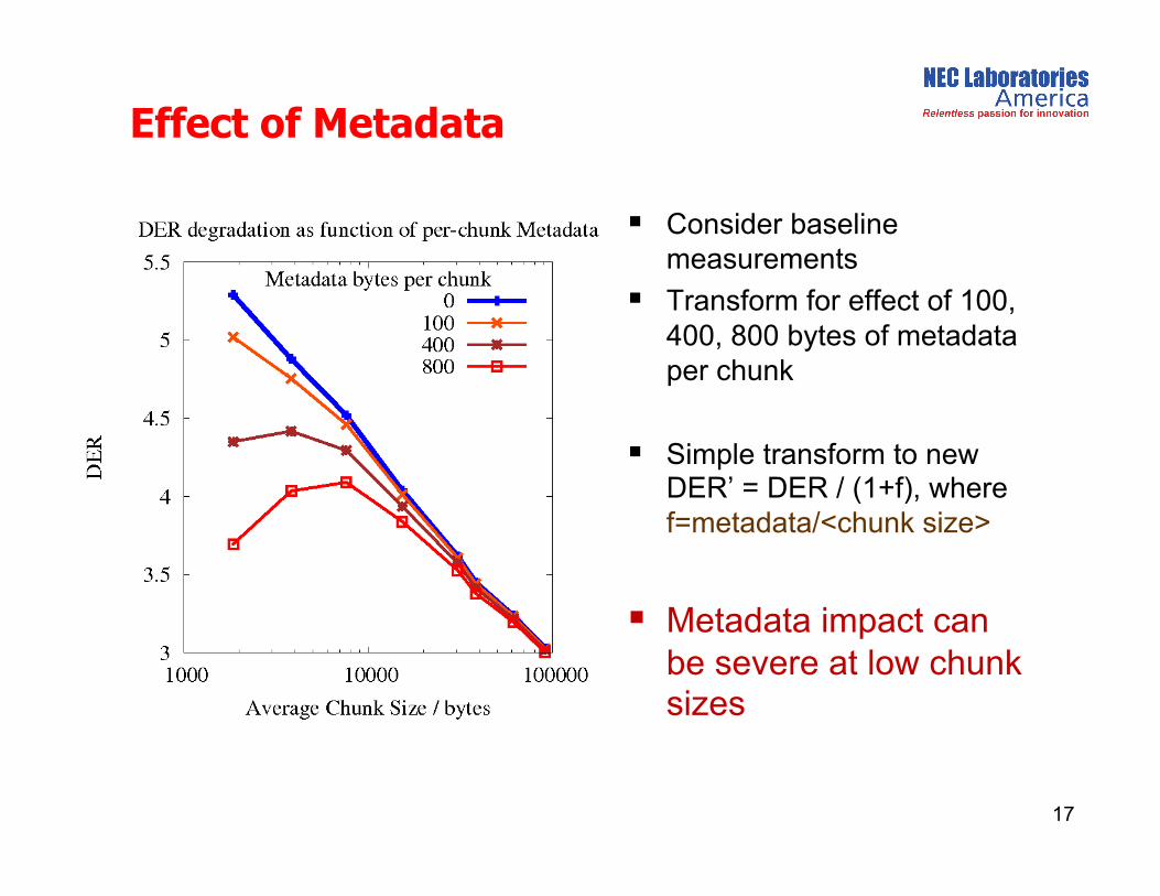
Effect of Metadata
17
Consider baseline measurements
Transform for effect of 100, 400, 800 bytes of metadata per chunk
Simple transform to new DER’ = DER / (1+f), where f=metadata/<chunk size>
Metadata impact can be severe at low chunk sizes

Detailed results: breaking apart
18
Typical settings: Min:avg:max = 1:2:3
3 backup levels Small chunker settings
divided by 1:2:4:8
1 existence query per big chunk
Small chunker 4-8x smaller (on average) was a reasonable choice.
Variations on min:avg:max had little effect
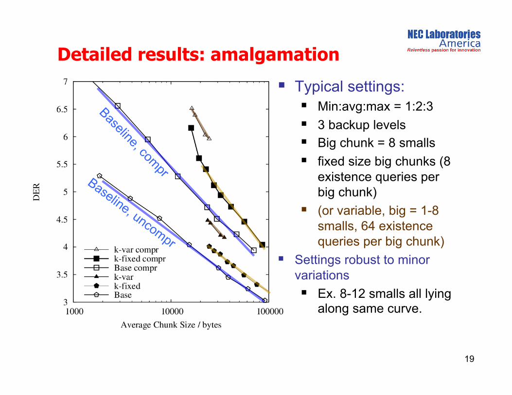
Detailed results: amalgamation
19
Typical settings: Min:avg:max = 1:2:3
3 backup levels Big chunk = 8 smalls
fixed size big chunks (8 existence queries per big chunk)
(or variable, big = 1-8 smalls, 64 existence queries per big chunk)
Settings robust to minor variations
Ex. 8-12 smalls all lying along same curve.

Intuitive model of file system backups 1. Long stretches of unseen data should be assumed to be
good candidates for appearing later on (i.e. at the next backup run).
2. Inefficiency around “change regions” straddling boundaries between duplicate and unseen data can be minimized by using shorter chunks.
• Confirmed by “oracle” experiments
“Historical” intuitions: beware!
20
• Experiment: • Run baseline chunker • Count (# dup, # following nondup) • Weight for # of bytes of input data
• Over these 14 backups, long stretches of unseen data were rather rare.
# dup
# following dup
Non-backup archives
21
Source code archives, ~ 10 or so versions Ran amalgamation with fixed-size big chunks of k smalls
Varied k
Gcc sources showed some small benefit, while emacs source showed no benefit. Not a universal solution
DER/chunk size gains definitely depend on nature of archive Expect problems if unimodal DER is low:
Ex: emacs uncompressed DER was only ~1.73 for <8k> chunks
One of our assumptions is failing --- duplication probability is never very high.
When blocks frequently fail assumption of “high probability to be seen later”, bimodal chunking may not be worthwhile.

Conclusions
22
For archival data with DER >3-4, “chunking transition regions small” is a useful mechanism to achieve competitive DER with larger than usual chunk sizes.
Transition regions can be determined by adding an existence query capability to existing block stores.
Small chunks in transition regions can show enhanced probability to be seen later.
Questions?