Bilinear and Trilinear Regression Models with Structured ...liu.diva-portal.org/smash/get/diva2:813054/FULLTEXT01.pdf · Models with Structured Covariance Matrices ... Alexandre Lyambabaje,

Linköping Studies in Science and Technology. Dissertations.No. 1665

Bilinear and Trilinear RegressionModels with Structured Covariance

Matrices

Joseph Nzabanita

Department of MathematicsLinköping University, SE–581 83 Linköping, Sweden

Linköping 2015

Linköping Studies in Science and Technology. Dissertations.No. 1665

Bilinear and Trilinear Regression Models with Structured Co variance Matrices

Joseph Nzabanita

[email protected]

Mathematical StatisticsDepartment of Mathematics

Linköping UniversitySE–581 83 Linköping

Sweden

ISBN 978-91-7519-070-9 ISSN 0345-7524

Copyright c© 2015 Joseph Nzabanita

Printed by LiU-Tryck, Linköping, Sweden 2015

To my Family and Friends

Abstract

Joseph Nzabanita (2015). Bilinear and Trilinear Regression Models withStructured Covariance Matrices

Doctoral dissertation. ISBN 978-91-7519-070-9 . ISSN 0345-7524.

This thesis focuses on the problem of estimating parametersin bilinear and trilinear re-gression models in which random errors are normally distributed. In these models thecovariance matrix has a Kronecker product structure and some factor matrices may belinearly structured. Most of techniques in statistical modeling rely on the assumption thatdata were generated from the normal distribution. Whereas real data may not be exactlynormal, the normal distributions serve as a useful approximation to the true distribution.The modeling of normally distributed data relies heavily onthe estimation of the meanand the covariance matrix. The interest of considering various structures for the covari-ance matrices in different statistical models is partly driven by the idea that altering thecovariance structure of a parametric model alters the variances of the model’s estimatedmean parameters.

Firstly, we consider the extended growth curve model with a linearly structured co-variance matrix. In general there is no problem to estimate the covariance matrix whenit is completely unknown. However, problems arise when one has to take into accountthat there exists a structure generated by a few number of parameters. An estimation pro-cedure that handles linear structured covariance matricesis proposed. The idea is firstto estimate the covariance matrix when it may be used to definean inner product in aregression space and thereafter re-estimate it when it should be interpreted as a dispersionmatrix. This idea is exploited by decomposing the residual space, the orthogonal comple-ment to the design space, into orthogonal subspaces. Studying residuals obtained fromprojections of observations on these subspaces yields explicit consistent estimators of thecovariance matrix. An explicit consistent estimator of themean is also proposed.

Secondly, we study a bilinear regression model with matrix normally distributed ran-dom errors. For those models, the dispersion matrix followsa Kronecker product structureand it can be used, for example, to model data with spatio-temporal relationships. Theaim is to estimate the parameters of the model when, in addition, one covariance matrixis assumed to be linearly structured. On the basis ofn independent observations from amatrix normal distribution, estimating equations, a flip-flop relation, are established.

At last, the models based on normally distributed random third order tensors are stud-ied. These models are useful in analyzing 3-dimensional data arrays. The 3-dimensionaldata arrays may be obtained when, for example, a single response is sampled in a 3-Dspace or in a 2-D space and time, multiple responses are recorded in a 2-D space or in a1-D space and time. In some studies the analysis is done usingthe tensor normal model,where the focus is on the estimation of the variance-covariance matrix which has a Kro-necker structure. Little attention is paid to the structureof the mean, however, there is apotential to improve the analysis by assuming a structured mean. We formally introducea 2-fold growth curve model by assuming a trilinear structure for the mean in the tensornormal model and propose an estimation algorithm for parameters. Also some extensionsare discussed.

v

Populärvetenskaplig sammanfattning

Många statistiska modeller bygger på antagandet om normalfördelad data. Verklig datakanske inte är exakt normalfördelad men det är i många fall enbra approximation. Nor-malfördelad data kan modelleras enbart genom dess väntevärde och kovariansmatris ochdet är därför ett problem av stort intresse att skatta dessa parametrar. Ofta kan det ock-så vara intressant eller nödvändigt att anta någon strukturpå både väntevärdet och/ellerkovariansmatrisen.

Den här avhandlingen fokuserar på problemet att skatta parametrarna i multivaria-ta linjära modeller, speciellt den utökade tillväxtkurvemodellen med en linjär strukturför någon kovariansmatris. I allmänhet är det inget problematt skatta kovariansmatriser-na när de är helt okända. Problem uppstår emellertid när man måste ta hänsyn till attdet finns en struktur som genereras av ett färre antal parametrar. I många exempel kanmaximum-likelihoodskattningar inte erhållas explicit och måste därför beräknas med nå-gon numerisk optimeringsalgoritm. Vi beräknar explicita skattningar som ett bra alternativtill maximum-likelihoodskattningarna. En skattningsprocedur som skattar kovariansma-triser med linjära strukturer föreslås. Tanken är att förstskatta en kovariansmatris somanvänds för att definiera en inre produkt, för att sedan skatta den slutliga kovariansmatri-sen.

Även tillväxtkurvemodeller med tensornormalfördelning studeras i den här avhand-lingen. För dessa modeller är kovariansmatrisen en Kroneckerprodukt och dessa modellerkan användas exempelvis för att modellera data med spatio-temporala förhållande. Syftetär att skatta parametrarna i modellen där möjligen även en avkovariansmatriserna antasfölja en linjär struktur.

vii

Acknowledgments

My deepest gratitude goes first to my supervisors Professor Dietrich von Rosen and DrMartin Singull for their invaluable guidance, encouragement and insightful ideas on sci-entific matters without which this thesis would not be completed. Thank you Dietrich,thank you Martin. The patience, the enthusiasm and many morehumane qualities youconstantly show helped me a lot during my studies.

My deep gratitude goes to Bengt Ove Turesson, to Björn Textorius, to MagnusHerberthson, to Fredrik Berntsson, to Göran Forsling, to Tomas Sjödin, to TheresiaCarlsson Roth, to Theresa Lagali and to all members of the Department of Mathematics,Linköping University, for their constant help in differentthings.

I am thankful to the staff of the University of Rwanda, especially FrodualdMinani, Alexandre Lyambabaje, Raymond Ndikumana, Alex Karara, Colin Karuhangaand Charles Gakomeye for their invaluable contribution to the smooth running of mystudies.

I have also to thank my fellow PhD students at the Department of Mathematics formaking life easier during my studies.

Last but not least, I owe my special thanks to my family and friends for moral supportand distraction.

My studies have been supported by the UR-Sweden Programme for Research, HigherEducation and Institutional Advancement and all involved institutions and people are ac-knowledged.

Linköping, May 6, 2015

Joseph Nzabanita

ix

Contents

1 Introduction 11.1 Background . . . . . . . . . . . . . . . . . . . . . . . . . . . . . . . . . 11.2 Aims . . . . . . . . . . . . . . . . . . . . . . . . . . . . . . . . . . . . . 21.3 Outline . . . . . . . . . . . . . . . . . . . . . . . . . . . . . . . . . . . 2

1.3.1 Outline of Part I . . . . . . . . . . . . . . . . . . . . . . . . . . 21.3.2 Outline of Part II . . . . . . . . . . . . . . . . . . . . . . . . . . 3

I Bilinear and Trilinear Regression Models 5

2 Multivariate Distributions 72.1 Normal distributions . . . . . . . . . . . . . . . . . . . . . . . . . . . . 72.2 Wishart distribution . . . . . . . . . . . . . . . . . . . . . . . . . . . . .12

3 Regression Models 153.1 General linear regression model . . . . . . . . . . . . . . . . . . . .. . 153.2 Bilinear regression models. Growth curve models . . . . . .. . . . . . . 163.3 Trilinear regression model . . . . . . . . . . . . . . . . . . . . . . . .. 193.4 Estimation in bilinear regression models . . . . . . . . . . . .. . . . . . 21

3.4.1 Maximum likelihood estimators . . . . . . . . . . . . . . . . . . 213.4.2 Explicit estimators when the covariance matrix is linearly structured 24

3.5 Estimation in trilinear regression model . . . . . . . . . . . .. . . . . . 28

4 Concluding Remarks 314.1 Summary of contributions . . . . . . . . . . . . . . . . . . . . . . . . . 314.2 Further research . . . . . . . . . . . . . . . . . . . . . . . . . . . . . . . 32

xi

xii Contents

Bibliography 33

II Papers 37

A Paper A 391 Introduction . . . . . . . . . . . . . . . . . . . . . . . . . . . . . . . . . 422 Maximum likelihood estimators . . . . . . . . . . . . . . . . . . . . . . 433 Estimators in the extended growth curve model with a linearly structured

covariance matrix . . . . . . . . . . . . . . . . . . . . . . . . . . . . . . 464 Properties of the proposed estimators . . . . . . . . . . . . . . . . .. . . 515 Numerical examples . . . . . . . . . . . . . . . . . . . . . . . . . . . . 54References . . . . . . . . . . . . . . . . . . . . . . . . . . . . . . . . . . . . . 58

B Paper B 611 Introduction . . . . . . . . . . . . . . . . . . . . . . . . . . . . . . . . . 642 Main idea and space decomposition . . . . . . . . . . . . . . . . . . . . 653 Estimators when the covariance matrix is linearly structured . . . . . . . 694 Simulation study . . . . . . . . . . . . . . . . . . . . . . . . . . . . . . 75

4.1 Procedures and methods . . . . . . . . . . . . . . . . . . . . . . 754.2 Results . . . . . . . . . . . . . . . . . . . . . . . . . . . . . . . 77

References . . . . . . . . . . . . . . . . . . . . . . . . . . . . . . . . . . . . . 77

C Paper C 791 Introduction . . . . . . . . . . . . . . . . . . . . . . . . . . . . . . . . . 822 Explicit estimators of linearly structuredΣ with unknown parameters and

knownΨ . . . . . . . . . . . . . . . . . . . . . . . . . . . . . . . . . . 823 Estimators of linearly structuredΣ with unknown parameters and un-

knownΨ . . . . . . . . . . . . . . . . . . . . . . . . . . . . . . . . . . 844 Simulated numerical example . . . . . . . . . . . . . . . . . . . . . . . . 91References . . . . . . . . . . . . . . . . . . . . . . . . . . . . . . . . . . . . . 91

D Paper D 931 Introduction . . . . . . . . . . . . . . . . . . . . . . . . . . . . . . . . . 962 The tensor normal distribution with a structured mean . . . .. . . . . . . 963 Maximum likelihood estimation . . . . . . . . . . . . . . . . . . . . . . 99

3.1 Estimation of parameters in the 2-fold Growth Curve Model . . . 993.2 Estimation of parameters in the 2-fold Growth Curve Model when

Σ has a uniform structure . . . . . . . . . . . . . . . . . . . . . 1023.3 Estimation ofB, Σ, Ψ andΩ: General case . . . . . . . . . . . 103

4 Simulation study . . . . . . . . . . . . . . . . . . . . . . . . . . . . . . 1054.1 Procedures . . . . . . . . . . . . . . . . . . . . . . . . . . . . . 1054.2 Results . . . . . . . . . . . . . . . . . . . . . . . . . . . . . . . 106

References . . . . . . . . . . . . . . . . . . . . . . . . . . . . . . . . . . . . . 107

1Introduction

THE goals of statistical sciences are about planning experiments, setting up models toanalyze experiments and to study properties of these models. Statistical applica-

tion is about connecting statistical models to data. Statistical models are essentially formaking predictions; they form the bridge between observed data and unobserved (future)outcomes (Kattan and Gönen, 2008). The general statisticalparadigm constitutes of thefollowing steps: (i) set up a model, (ii) evaluate the model via simulations or comparisonswith data, (iii) if necessary refine the model and restart from step (ii), and (iv) accept andinterpret the model. From this paradigm it is clear that the concept of statistical model liesin the heart of Statistics. In this thesis our focus is on linear models, a class of statisticalmodels that play a key role in statistics. If exact inferenceis not possible then at least alinear approximate approach can often be carried out (Kolloand von Rosen, 2005). Inparticular, we are concerned with the problem of estimatingparameters in multivariatelinear normal models with structured mean (bilinear and trilinear regression models) andstructured covariance matrices (Kronecker and linear structures).

1.1 Background

Regression analysis includes several statistical techniques for investigating dependenciesamong variables. It is used essentially when the focus is to understand the relationshipsbetween a set of dependent variables and a set of independentvariables. The regressionanalysis appeared in earliest form as the method of least squares in the beginning ofthe nineteenth-century, where Legendre and Gauss applied the method to the problem ofdetermining orbits of comets and planets about the sun from astronomical observations.The term "regression" was introduced in late nineteenth-century by Francis Galton whilehe was studying the inheritance problem (Allen, 1997).

Although regression methods are in use since the last two centuries, there are stillinteresting problems that makes regression analysis to be an area of active research nowa-

1

2 1 Introduction

days. The newest research directions include regression involving correlated responsessuch as time series and growth curves, and the focus of this thesis can be traced there.

In regression models often one assumes that the underlying random errors follow aGaussian distribution. When the set up of the model is matrix or tensor, it becomes naturalto model the covariance matrix with a Kronecker product structure. For some other struc-tures for the covariance matrix, there might be theoreticalground to justify a particularchoice of the covariance structure (Fitzmaurice et al., 2012). In particular, the linear struc-tures for the covariance matrices emerged naturally in statistical applications and they arein the statistical literature for some years ago. These structures are, for example, uniformstructure, also known as intraclass structure, compound symmetry structure, banded ma-trix, Toeplitz or circular Toeplitz, etc. The uniform structure, a linear covariance structurewhich consists of equal diagonal elements and equal off-diagonal elements, emerged forthe first time in (Wilks, 1946) while dealing with measurements onk psychological tests.An extension of the uniform structure due to Votaw (1948) is the compound symmetrystructure, which consists of blocks each having uniform structure. In (Votaw, 1948) onecan find examples of psychometric and medical research problems where the compoundsymmetry covariance structure is applicable. The block compound symmetry covariancestructure was discussed by Szatrowski (1982) who applied the model to the analysis of aneducational testing problem. Ohlson et al. (2011) proposeda procedure to obtain explicitestimator of a banded covariance matrix. The Toeplitz or circular Toeplitz discussed in(Olkin and Press, 1969) is another generalizations of the intraclass structure. The interestof considering various structures for the covariance matrices in different statistical modelsis partly driven by the idea that altering the covariance structure of a parametric modelalters the variances of the model’s estimated mean parameters (Lange and Laird, 1989).

1.2 Aims

The main theme of this thesis is to study the problem of estimation of parameters inthe bilinear and trilinear regression models with structured covariance matrices. Specificobjectives are (i) to derive explicit estimators of parameters in the extended growth curvemodel when the covariance matrix is linearly structured, (ii) to propose an algorithmfor estimating parameters in the bilinear regression modelwhere the random errors areassumed to be matrix normally distributed with one linearlystructured covariance matrix,and (iii) to extend the classical growth curve model by Pothoff and Roy (1964) to a tensorversion and to propose an algorithm for estimating model parameters.

1.3 Outline

This thesis consists of two parts and the outline is as follows.

1.3.1 Outline of Part I

In Part I the background and relevant results that are neededfor an easy reading of thisthesis are presented. Part I starts with Chapter 2 which gives a brief review on the multi-variate distributions. The main focus is to define the matrixnormal distribution, the tensor

1.3 Outline 3

normal distribution and the Wishart distribution. The maximum likelihood estimators inthe multivariate normal model, the matrix normal model and the tensor normal model, forthe unstructured cases, are given. In Chapter 3 the bilinearand trilinear regression modelsare defined. These models include the growth curve model and the extended growth curvemodel, which are refereed to as bilinear regression models,and the third order tensor nor-mal model with a structured mean refereed to as the trilinearregression model. Someresults on the estimation of parameters in the extended growth curve model are givenfor unstructured covariance matrix and the procedure to getexplicit estimators when thecovariance matrix is linearly structured is illustrated. Also, an algorithm for estimatingparameters in the trilinear regression model is given. PartI ends with Chapter 4, whichgives a summary of contributions and suggestions for further work.

1.3.2 Outline of Part II

Part II consists of four papers. Hereafter a short summary for the papers is presented.

Paper A: Estimation of parameters in the extended growth curvemodel with a linearly structured covariance matrix

Nzabanita, J., Singull, M., and von Rosen, D. (2012). Estimation of parame-ters in the extended growth curve model with a linearly structured covariancematrix. Acta et Commentationes Universitatis Tartuensis de Mathematica,16(1):13–32.

In Paper A, the extended growth curve model with two terms anda linearly structuredcovariance matrix is considered. We propose an estimation procedure that handles linearstructured covariance matrices. The idea is first to estimate the covariance matrix when itshould be used to define an inner product in a regression spaceand thereafter re-estimateit when it should be interpreted as a dispersion matrix. Thisidea is exploited by de-composing the residual space, the orthogonal complement tothe design space, into threeorthogonal subspaces. Studying residuals obtained from projections of observations onthese subspaces yields explicit consistent estimators of the covariance matrix. An explicitconsistent estimator of the mean is also proposed and numerical examples are given.

Paper B: Extended GMANOVA model with a linearly structuredcovariance matrix

Nzabanita, J., von Rosen, D., and Singull, M. (2015a). Extended GMANOVAmodel with a linearly structured covariance matrix.Linköping UniversityElectronic Press, LiTH-MAT-R-2015/07-SE.

Paper B generalizes results in Paper A to the extended GMANOVA model with an ar-bitrary number of profiles, saym. We show how to decompose the residual space, theorthogonal complement to the mean space, intom + 1 orthogonal subspaces and howto derive explicit consistent estimators of the covariancematrix and an explicit unbiasedestimator of the mean.

4 1 Introduction

Paper C: Bilinear regression model with Kronecker and linearstructures for the covariance matrix

Nzabanita, J. (2013). Multivariate linear models with kronecker product andlinear structures on the covariance matrices. InProceedings, JSM 2013-IMS,pp. 1582–1588. Alexandria, VA: American Statistical Association.(A pre-liminary version).

This paper deals with models based on normally distributed random matrices. Morespecifically the model considered isX ∼ Np,q(M ,Σ,Ψ) with meanM , a p × q ma-trix, assumed to follow a bilinear structure, i.e.,E[X] = M = ABC, whereA andCare known design matrices,B is unkown parameter matrix, and the dispersion matrix ofX has a Kronecker product structure, i.e.,D[X] = Ψ ⊗ Σ, where bothΨ andΣ areunknown positive definite matrices. The model may be used forexample to model datawith spatio-temporal relationships. The aim is to estimatethe parameters of the modelwhen, in addition,Σ is assumed to be linearly structured. In the paper, on the basis ofn independent observations on the random matrixX, estimation equations in a flip-floprelation are presented and the consistency of estimators isstudied.

Paper D: Maximum likelihood estimation in the tensor normalmodel with a structured mean

Nzabanita, J., von Rosen, D., and Singull, M. (2015b). Maximum likelihoodestimation in the tensor normal model with a structured mean. LinköpingUniversity Electronic Press, LiTH-MAT-R-2015/08-SE.

In this paper, we introduce a 2-fold growth curve model by assuming a trilinear structurefor the mean in the tensor normal model. More specifically, the model considered may bewritten as

X = B × A,C,D+ E ,

whereX : p× q × r is the data tensor,B : s× t× u is the parameter given as a tensorof order three,A : p × s, C : q × t andD : r × u are known design matrices, and× denotes the Tucker product. The random errors follow a tensor normal distributionwith mean zero, i.e.,E ∼ Np,q,r(O,Σ,Ψ, Ir), andO is a tensor of zeros. An algorithmfor estimating parameters is proposed and some direct generalizations of the model arepresented.

Part I

Bilinear and TrilinearRegression Models

5

2Multivariate Distributions

THIS chapter focuses on the normal distribution which is very important in statisticalanalysis. In particular, our interest here is to define the matrix and tensor normal

distributions which will play a central role in this thesis.The Wishart distribution willalso be looked at for easy reading of papers.

2.1 Normal distributions

The well known univariate normal distribution has been usedin statistics for about twohundreds years and the multivariate normal distribution, understood as a distribution of avector, has been also used for a long time (Kollo and von Rosen, 2005). Due to the com-plexity of data from various field of applied research, inevitable extensions of the multi-variate normal distribution to the matrix normal distribution or even more generalizationto multilinear (tensor) normal distribution have been considered. The normal distributionswe present here exclude the degenerate cases and thus their density functions exist.

Definition 2.1 (Univariate normal distribution). A random variablex is a univariatenormal distribution with meanµ ∈ R and varianceσ2 > 0, denoted asx ∼ N

(µ, σ2

)if

its density is

f(x) =1

σ√2πe−

(x−µ)2

2σ2 , (−∞ < x <∞) .

In particular whenµ = 0 andσ = 1, we get the standard univariate normal dis-tribution, i.e.,u ∼ N (0, 1). A more general characterization of the univariate normaldistribution is

xd= µ+ σu, µ ∈ R, σ ≥ 0,

whereu ∼ N (0, 1) and the notation "d=" means "has the same distribution as".

7

8 2 Multivariate Distributions

Definition 2.2 (Multivariate normal distribution). A random vectorx : p× 1 is mul-tivariate normally distributed with mean vectorµ : p× 1 and positive definite covariancematrixΣ : p× p if its density is

f(x) = (2π)− p

2 |Σ|− 12 e−

12 trΣ

−1(x−µ)(x−µ)′,

where| · | andtr denote the determinant and the trace of a matrix, respectively. We usuallyuse the notationx ∼ Np(µ,Σ).

The multivariate normal modelx ∼ Np(µ,Σ), whereµ andΣ are unknown pa-rameters, is used in the statistical literature for a long time. To find estimators of theparameters, the method of maximum likelihood is often used.Let a random sample ofnobservation vectorsx1,x2, . . . ,xn come from the multivariate normal distribution, i.e.,xi ∼ Np(µ,Σ). Thexi’s constitute a random sample and the likelihood function isgivenby the product of the densities evaluated at each observation vector

L(x1,x2, . . . ,xn,µ,Σ) =n∏

i=1

f(xi,µ,Σ)

=

n∏

i=1

(2π)− p

2 |Σ|− 12 e−

12 trΣ

−1(xi−µ)(xi−µ)′.

The maximum likelihood estimators (MLEs) ofµ andΣ resulting from the maximizationof this likelihood function, for more details see for example Johnson and Wichern (2007),are respectively

µ =1

n

n∑

i=1

xi =1

nX1n,

Σ =1

nS,

where

S =n∑

i=1

(xi − µ)(xi − µ)′ = X(In − 1

n1n1

′n)X

′,

X = (x1,x2, . . . ,xn), 1n is then−dimensional vector of 1’s, andIn is then × nidentity matrix.

Definition 2.3 (Matrix normal distribution). A random matrixX : p × q is matrixnormally distributed with meanM : p × q and positive definite covariance matricesΣ : p× p andΨ : q × q if its density is

f(X) = (2π)− pq

2 |Σ|− q2 |Ψ|− p

2 e−12 trΣ

−1(X−M)Ψ−1(X−M)′.

The model based on the matrix normally distributed is usually denoted as

X ∼ Np,q(M ,Σ,Ψ), (2.1)

2.1 Normal distributions 9

and it can be shown thatX ∼ Np,q(M ,Σ,Ψ) means the same as

vecX ∼ Npq(vecM ,Ψ⊗Σ), (2.2)

where⊗ denotes the Kronecker product. Since by definition of the dispersion matrix ofX isD[X] = D[vecX], we getD[X] = Ψ ⊗Σ. For the interpretation we note thatΨ

describes the covariances between the columns ofX. These covariances will be the samefor each row ofX. The other covariance matrixΣ describes the covariances betweenthe rows ofX which will be the same for each column ofX. The productΨ ⊗Σ takesinto account the covariances between columns as well as the covariances between rows.Therefore,Ψ ⊗ Σ indicates that the overall covariance consists of the products of thecovariances inΨ and inΣ, respectively, i.e.,Cov[xij , xkl] = σikψjl, whereX = (xij),Σ = (σik) andΨ = (ψjl).

The following example shows one possibility of how a matrix normal distribution mayarise.

Example 2.1

Let x1, . . . ,xn be an independent sample ofn observation vectors from a multivariatenormal distributionNp (µ,Σ) and let the observation vectorsxi be the columns in amatrixX = (x1,x2, . . . ,xn). The distribution of the vectorization of the sample obser-vation matrixvecX is given by

vecX = (x′1, x

′2, . . . ,x

′n)

′ ∼ Npn (1n ⊗ µ,Ω) ,

whereΩ = In ⊗Σ, 1n is then−dimensional vector of 1s, andIn is then × n identitymatrix. This is written as

X ∼ Np,n (M ,Σ, In) ,

whereM = µ1′n.

The models (2.1) and (2.2) have been considered in the statistical literature. For exam-ple Dutilleul (1999), Roy and Khattree (2005) and Lu and Zimmerman (2005) consideredthe model (2.2), and to obtain MLEs these authors solved iteratively the usual likelihoodequations, one obtained by assuming thatΨ is given and the other obtained by assumingthatΣ is given, by what was called the flip-flop algorithm in Lu and Zimmerman (2005).

Let a random sample ofn observation matricesX1,X2, . . . ,Xn be drawn from thematrix normal distribution, i.e.,Xi ∼ Np(M ,Σ,Ψ). The likelihood function is givenby the product of the densities evaluated at each observation matrix as it was for themultivariate case. The log-likelihood, ignoring the normalizing factor, is given by

lnL(X,M ,Σ,Ψ) = −qn2

ln |Σ| − pn

2ln |Ψ|

−1

2

n∑

i=1

trΣ−1(Xi −M)Ψ−1(Xi −M)′.


The likelihood equations are given by Dutilleul (1999)

M =1

n

n∑

i=1

Xi = X;

Σ =1

nq

n∑

i=1

(Xi − M)Ψ−1

(Xi − M)′;

Ψ =1

np

n∑

i=1

(Xi − M)′Σ−1

(Xi − M).

There is no explicit solutions to these equations and one must rely on an iterative algo-rithm like the flip-flop algorithm (Dutilleul, 1999). Srivastava et al. (2008) pointed outthat the estimators found in this way are not uniquely determined. Srivastava et al. (2008)showed that solving these equations with additional estimability conditions, using the flip-flop algorithm, the estimates in the algorithm converge to the unique maximum likelihoodestimators of the parameters.

The model (2.1), where the mean has a bilinear structure was considered by Srivastavaet al. (2008). Nzabanita (2013) considered the problem of estimating the parameters inthe model (2.1) where the mean has a bilinear structure and, in addition, the covariancematrixΣ is assumed to be linearly structured.

A matrix normal model may be thought as a two-array normal model and can be ex-tended to aK-array normal model (also known as tensor normal model). Before we givea formal definition of aK-array normal model, we first introduce few notations and op-erations onK-arrays to be used later. AK-array orK-way orKth-order tensor is anelement of the tensor product ofK vector spaces, each of which has its own coordinatesystem (Hoff, 2011, Kolda and Bader, 2009, De Lathauwer et al., 2000). For example, avectorx ∈ Rp1 is a one-array with dimensionp1. A matrix X ∈ Rp1×p2 is a two-arraywith dimension(p1, p2). An arrayX ∈ Rp1×p2×···×pK is aK-array with dimension(p1, . . . , pK) and has elementsxi1,...,iK : ik ∈ 1, . . . , pk, k = 1, . . . ,K. A matri-cization or unfolding or flattening of a tensor is the processof reordering its elements intoa matrix. This can be done in several ways. In this thesis we use the so called mode-nmatricization and the notationX(n) is used to denoten-mode matrix from the tensorX .For some details about matricization and decomposition of tensors refer to (Hoff, 2011,Kolda and Bader, 2009, De Lathauwer et al., 2000). A vectorization ofX is defined withhelp of usualvec operator for matrices asvecX = vecX(1).

Definition 2.4 (Tensor normal distribution). A randomKth order tensorX ∈ Rp1×p2×···×pK

is said to be normally distributed if

Xd= M + U × τ 1, τ 2, . . . , τK,

for someM ∈ Rp1×p2×···×pK , non-singular matricesτ k ∈ Rpk×pk , k = 1, . . . ,K anda random tensorU ∈ Rp1×p2×···×pK with i.i.d. standard normal entries.

Here, the symbol "×" denotes the Tucker product (Tucker, 1964, Kolda and Bader,2009) defined by the identity

vec(U × τ 1, τ 2, . . . , τK) = (τK ⊗ τK−1 ⊗ . . .⊗ τ 1)vecU .

2.1 Normal distributions 11

It follows that

E[X ] = M , D[X ] = D[vecX ] = τKτ ′K ⊗ τK−1τ

′K−1 ⊗ . . .⊗ τ 1τ

′1.

Thus, the tensor normal distribution corresponds to the multivariate normal distributionwith separable (Kronecker product structure) covariance matrix. LettingΣk = τ kτ

′k, we

write

X ∼ Np1,...,pK(M ,Σ1, . . . ,ΣK), (2.3)

which is equivalent tovecX ∼ Np1···pK(vecM ,ΣK ⊗ · · · ⊗Σ1). The density function

is given by

f(x) = (2π)−p/2

(K∏

k=1

|Σk|−p/(2pk)

)exp

−1

2(x− µ)′Σ−1

1:K(x− µ)

,

whereΣ1:K = Σ1 ⊗ · · · ⊗ΣK , x = vecX , µ = vecM andp =∏K

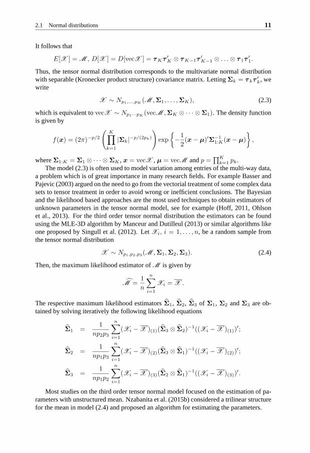
k=1 pk.The model (2.3) is often used to model variation among entries of the multi-way data,

a problem which is of great importance in many research fields. For example Basser andPajevic (2003) argued on the need to go from the vectorial treatment of some complex datasets to tensor treatment in order to avoid wrong or inefficient conclusions. The Bayesianand the likelihood based approaches are the most used techniques to obtain estimators ofunknown parameters in the tensor normal model, see for example (Hoff, 2011, Ohlsonet al., 2013). For the third order tensor normal distribution the estimators can be foundusing the MLE-3D algorithm by Manceur and Dutilleul (2013) or similar algorithms likeone proposed by Singull et al. (2012). LetXi, i = 1, . . . , n, be a random sample fromthe tensor normal distribution

X ∼ Np1,p2,p3(M ,Σ1,Σ2,Σ3). (2.4)

Then, the maximum likelihood estimator ofM is given by

M =1

n

n∑

i=1

Xi = X .

The respective maximum likelihood estimatorsΣ1, Σ2, Σ3 of Σ1, Σ2 andΣ3 are ob-tained by solving iteratively the following likelihood equations

Σ1 =1

np2p3

n∑

i=1

(Xi − X )(1)(Σ3 ⊗ Σ2)−1((Xi − X )(1))

′;

Σ2 =1

np1p3

n∑

i=1

(Xi − X )(2)(Σ3 ⊗ Σ1)−1((Xi − X )(2))

′;

Σ3 =1

np1p2

n∑

i=1

(Xi − X )(3)(Σ2 ⊗ Σ1)−1((Xi − X )(3))

′.

Most studies on the third order tensor normal model focused on the estimation of pa-rameters with unstructured mean. Nzabanita et al. (2015b) considered a trilinear structurefor the mean in model (2.4) and proposed an algorithm for estimating the parameters.


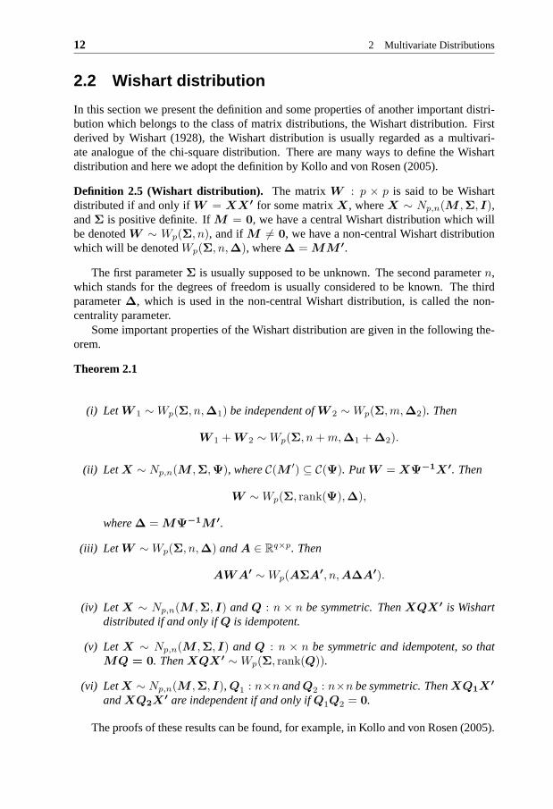
2.2 Wishart distribution

In this section we present the definition and some propertiesof another important distri-bution which belongs to the class of matrix distributions, the Wishart distribution. Firstderived by Wishart (1928), the Wishart distribution is usually regarded as a multivari-ate analogue of the chi-square distribution. There are manyways to define the Wishartdistribution and here we adopt the definition by Kollo and vonRosen (2005).

Definition 2.5 (Wishart distribution). The matrixW : p × p is said to be Wishartdistributed if and only ifW = XX′ for some matrixX, whereX ∼ Np,n(M ,Σ, I),andΣ is positive definite. IfM = 0, we have a central Wishart distribution which willbe denotedW ∼ Wp(Σ, n), and ifM 6= 0, we have a non-central Wishart distributionwhich will be denotedWp(Σ, n,∆), where∆ = MM ′.

The first parameterΣ is usually supposed to be unknown. The second parametern,which stands for the degrees of freedom is usually considered to be known. The thirdparameter∆, which is used in the non-central Wishart distribution, is called the non-centrality parameter.

Some important properties of the Wishart distribution are given in the following the-orem.

Theorem 2.1

(i) LetW 1 ∼Wp(Σ, n,∆1) be independent ofW 2 ∼Wp(Σ,m,∆2). Then

W 1 +W 2 ∼Wp(Σ, n+m,∆1 +∆2).

(ii) Let X ∼ Np,n(M ,Σ,Ψ), whereC(M ′) ⊆ C(Ψ). PutW = XΨ−1X′. Then

W ∼Wp(Σ, rank(Ψ),∆),

where∆ = MΨ−1M ′.

(iii) Let W ∼Wp(Σ, n,∆) andA ∈ Rq×p. Then

AWA′ ∼Wp(AΣA′, n,A∆A′).

(iv) LetX ∼ Np,n(M ,Σ, I) andQ : n × n be symmetric. ThenXQX′ is Wishartdistributed if and only ifQ is idempotent.

(v) LetX ∼ Np,n(M ,Σ, I) andQ : n × n be symmetric and idempotent, so thatMQ = 0. ThenXQX′ ∼Wp(Σ, rank(Q)).

(vi) LetX ∼ Np,n(M ,Σ, I),Q1 : n×n andQ2 : n×n be symmetric. ThenXQ1X′

andXQ2X′ are independent if and only ifQ1Q2 = 0.

The proofs of these results can be found, for example, in Kollo and von Rosen (2005).

2.2 Wishart distribution 13

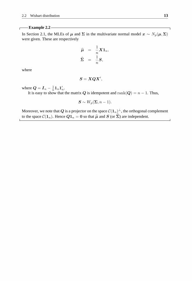
Example 2.2

In Section 2.1, the MLEs ofµ andΣ in the multivariate normal modelx ∼ Np(µ,Σ)were given. These are respectively

µ =1

nX1n,

Σ =1

nS,

where

S = XQX ′,

whereQ = In − 1n1n1

′n.

It is easy to show that the matrixQ is idempotent andrank(Q) = n− 1. Thus,

S ∼Wp(Σ, n− 1).

Moreover, we note thatQ is a projector on the spaceC(1n)⊥, the orthogonal complement

to the spaceC(1n). HenceQ1n = 0 so thatµ andS (or Σ) are independent.

3Regression Models

THE goal of this chapter is to give definitions and some results onmultivariate linearmodels. It starts with the general linear regression model,which includes well known

models like the univariate linear regression model, the analysis of variance model and theanalysis of covariance model. The multivariate counterpart includes the multivarate linearregression model, the multivariate analysis of variance and the multivariate analysis ofcovariance model. Then, the growth curve model and the extended growth curve model,which are refereed to as the bilinear regression models, arepresented. At last, we definethe trilinear regression model and give an example to illustrate its construction.

3.1 General linear regression model

In the general linear model (GLM) setup, a random set ofn correlated observations, anobservation vectorx′ = (x1, x2, . . . , xn), is related to a vector ofk parameters,β′ =(β1, β2, . . . , βk), through a known nonrandom design matrixC : k × n plus a randomvector of errorse : n×1, with mean zero,E(e) = 0, and covariance matrixcov(e) = Σ.Thus, the general linear model (GLM) is represented as

x′ = β′C + e′, E(e) = 0, cov(e) = Σ, (3.1)

whereβ andΣ are unkown parameters.The vector of parameters,β, can be fixed, random or both (mixed model). In this

thesis parameters are assumed to be fixed. The matricesC andΣ may have differentforms and depending on these forms model (3.1) includes wellknown models like theunivariate (linear) regression (UR) model, the analysis ofvariance (ANOVA) model andthe analysis of covariance (ANCOVA) model.

Different techniques to estimate model parameters and hypothesis testing exist. Forexample, when there is no assumption on the distribution ofx, one can use the generalized

15

16 3 Regression Models

least squares (GLS) theory and minimum quadratic norm unbiased estimation (MINQUE)theory (Rao and Toutenburg, 1995) to estimateβ andΣ .

In many statistical analysis, one assumes that the vectorx has a multivariate normaldistribution and model (3.1) becomes

x ∼ Nn(C′β,Σ), (3.2)

that is a multivariate normal model with mean vectorC ′β and covariance matrixΣ. Inthis case the maximum likelihood theory for estimation and hypothesis testing may beused.

Model (3.2) corresponds ton observations on a single dependent response variable.When one hasn independent observation vectors,xi = (x1i, x2i, . . . , xpi)

′, i = 1, . . . , n,onp correlated dependent response variables, model (3.2) generalizes to the model

X = BC +E, (3.3)

whereX : p × n, B : p × k, C : k × n, E ∼ Np,n(0,Σ, I). The matrixC is a knowndesign matrix, andB and the positive definite matrixΣ are unknown parameter matrices.

Again, depending on the forms ofC andΣ, model (3.3) includes known modelslike the multivarate (linear) regression (MR) model, the multivariate analysis of variance(MANOVA) model (Roy, 1957, Anderson, 1958) and the multivariate analysis of covari-ance (MANCOVA) model.

3.2 Bilinear regression models. Growth curve models

The growth curve analysis is a topic with many important applications within medicine,natural sciences, social sciences, etc. Growth curve analysis has a long history and twoclassical papers are Box (1950) and Rao (1958). In 1964 the well known paper by Pothoffand Roy (1964) extended the MANOVA model (3.3) to the model which was later termedthe growth curve model or the general MANOVA (GMANOVA).

Definition 3.1 (Growth curve model). Let X : p × n, A : p × q, q ≤ p, B : q × k,C : k × n, r(C) + p ≤ n, wherer( · ) represents the rank of a matrix. The growth curvemodel is given by

X = ABC +E, (3.4)

where columns ofE are assumed to be independently distributed as a multivariate nor-mal distribution with mean zero and a positive definite dispersion matrixΣ; i.e., E ∼Np,n(0,Σ, In).

The matricesA andC, often called respectively within-individuals and between-individuals design matrices, are known matrices whereas matricesB andΣ are unknownparameter matrices.

The paper by Pothoff and Roy (1964) is often considered to be the first where themodel was presented. The GMANOVA model was introduced to analyze growth in bal-anced repeated measures data. Several prominent authors wrote follow-up papers, e.g.,

3.2 Bilinear regression models. Growth curve models 17

Rao (1965) and Khatri (1966). Notice that the growth curve model is a special case of thematrix normal model where the mean has a bilinear structure.Therefore, we may use thenotation

X ∼ Np,n(ABC,Σ, I).

Also, it is worth noting that the MANOVA model with restrictions

X = BC +E, (3.5)

GB = 0

is equivalent to the growth curve model.GB = 0 is equivalent toB = (G′)oΘ, where(G′)o is any matrix spanning the orthogonal complement to the space generated by thecolumns ofG′. Plugging(G′)oΘ in (3.5) gives

X = (G′)oΘC +E,

which is identical to the growth curve model (3.4).

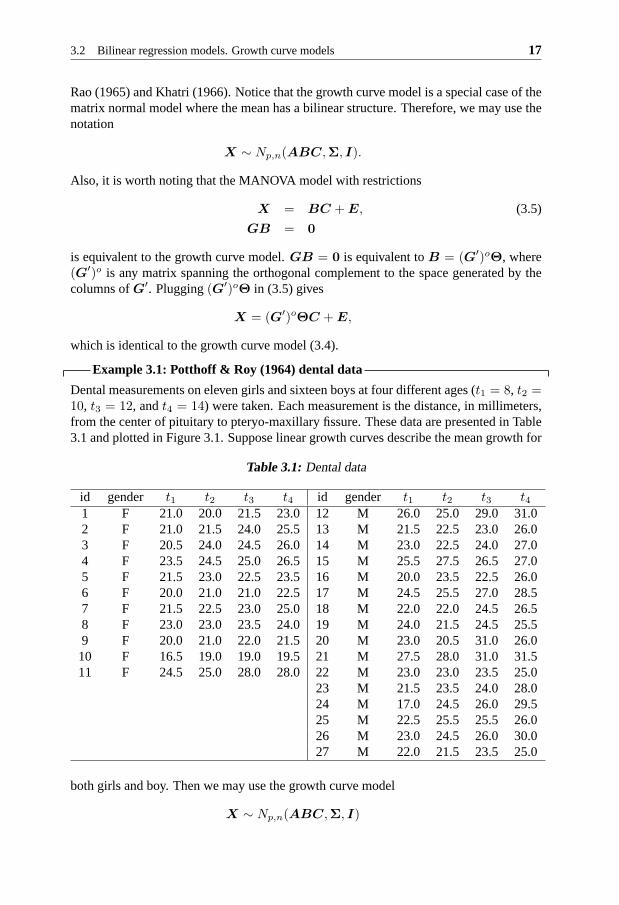
Example 3.1: Potthoff & Roy (1964) dental data

Dental measurements on eleven girls and sixteen boys at fourdifferent ages (t1 = 8, t2 =10, t3 = 12, andt4 = 14) were taken. Each measurement is the distance, in millimeters,from the center of pituitary to pteryo-maxillary fissure. These data are presented in Table3.1 and plotted in Figure 3.1. Suppose linear growth curves describe the mean growth for

Table 3.1: Dental data

id gender t1 t2 t3 t4 id gender t1 t2 t3 t41 F 21.0 20.0 21.5 23.0 12 M 26.0 25.0 29.0 31.02 F 21.0 21.5 24.0 25.5 13 M 21.5 22.5 23.0 26.03 F 20.5 24.0 24.5 26.0 14 M 23.0 22.5 24.0 27.04 F 23.5 24.5 25.0 26.5 15 M 25.5 27.5 26.5 27.05 F 21.5 23.0 22.5 23.5 16 M 20.0 23.5 22.5 26.06 F 20.0 21.0 21.0 22.5 17 M 24.5 25.5 27.0 28.57 F 21.5 22.5 23.0 25.0 18 M 22.0 22.0 24.5 26.58 F 23.0 23.0 23.5 24.0 19 M 24.0 21.5 24.5 25.59 F 20.0 21.0 22.0 21.5 20 M 23.0 20.5 31.0 26.010 F 16.5 19.0 19.0 19.5 21 M 27.5 28.0 31.0 31.511 F 24.5 25.0 28.0 28.0 22 M 23.0 23.0 23.5 25.0

23 M 21.5 23.5 24.0 28.024 M 17.0 24.5 26.0 29.525 M 22.5 25.5 25.5 26.026 M 23.0 24.5 26.0 30.027 M 22.0 21.5 23.5 25.0

both girls and boy. Then we may use the growth curve model

X ∼ Np,n(ABC,Σ, I)


1 1.5 2 2.5 3 3.5 416

18

20

22

24

26

28

30

32

Age

Gro

wth

mea

sure

men

ts

Girls profileBoys profile

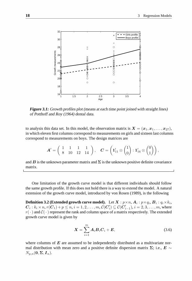
Figure 3.1: Growth profiles plot (means at each time point joined with straight lines)of Potthoff and Roy (1964) dental data.

to analysis this data set. In this model, the observation matrix is X = (x1,x1, . . . ,x27),in which eleven first columns correspond to measurements on girls and sixteen last columnscorrespond to measurements on boys. The design matrices are

A′ =

(1 1 1 18 10 12 14

), C =

(1′11 ⊗

(1

0

): 1′

16 ⊗(0

1

)),

andB is the unknown parameter matrix andΣ is the unknown positive definite covariancematrix.

One limitation of the growth curve model is that different individuals should followthe same growth profile. If this does not hold there is a way to extend the model. A naturalextension of the growth curve model, introduced by von Rosen(1989), is the following

Definition 3.2 (Extended growth curve model). LetX : p×n,Ai : p×qi,Bi : qi×ki,Ci : ki×n, r(C1)+ p ≤ n, i = 1, 2, . . . ,m, C(C ′

i) ⊆ C(C ′i−1), i = 2, 3, . . . ,m, where

r( · ) andC( · ) represent the rank and column space of a matrix respectively. The extendedgrowth curve model is given by

X =m∑

i=1

AiBiCi +E, (3.6)

where columns ofE are assumed to be independently distributed as a multivariate nor-mal distribution with mean zero and a positive definite dispersion matrixΣ; i.e., E ∼Np,n(0,Σ, In).

3.3 Trilinear regression model 19

The matricesAi andCi, often called design matrices, are known matrices whereasmatricesBi andΣ are unknown parameter matrices. As for the growth curve model thenotation

X ∼ Np,n

(m∑

i=1

AiBiCi,Σ, I

)

may be used for the extended growth curve model. The only difference with the growthcurve model in Definition 3.1 is the presence of a more generalmean structure. Whenm = 1, the model reduces to the growth curve model. The model without subspaceconditions was considered before by Verbyla and Venables (1988) under the name ofsum of profiles model. Also observe that the subspace conditionsC(C ′

i) ⊆ C(C ′i−1),

i = 2, 3, . . . ,m may be replaced byC(Ai) ⊆ C(Ai−1), i = 2, 3, . . . ,m. This problemwas considered for example by Filipiak and von Rosen (2012) form = 3.

Example 3.2Consider again Potthoff & Roy (1964) classical dental data.From Figure 3.1, it is rea-sonable to assume that for both girls and boys we have a lineargrowth component butadditionally for the boys there also exists a second order polynomial structure. Then wemay use the extended growth curve model with two terms

X ∼ Np,n(A1B1C1 +A2B2C2,Σ, I),

where

A′1 =

(1 1 1 18 10 12 14

), C1 =

(1′11 ⊗

(1

0

): 1′

16 ⊗(0

1

))

A′2 =

(82 102 122 142

), C2 = (0′

11 : 1′16),

are design matrices andB1 =

(β11 β12β21 β22

)andB2 = (β32) are parameter matrices and

Σ is the same as in Example 3.1.

3.3 Trilinear regression model

The classical growth curve model (3.4) by Pothoff and Roy (1964) comprises two designmatrices; one models the within-individuals structure whereas the other one models thebetween-individuals structure. More specifically, the within-individuals design matrixAcontains time regressors and models growth curves, and the between-individuals designmatrix C is comprised of group separation indicators. It is suitableto analyze, for ex-ample, "one directional" repeated measures data. Nzabanita et al. (2015b) extended theclassical growth curve model with an additional within-individuals design matrix whichcan be used to analyze "two directional" repeated measures data. More specifically, themodel considered is the third order tensor normal model

X ∼ Np,q,r(M ,Σ,Ψ,Ω),


with mean structure of the form

µijk =

s∑

ℓ=1

t∑

m=1

u∑

n=1

bℓmnaiℓcjmdkn, i = 1, . . . , p, j = 1, . . . , q, k = 1, . . . , r.

This mean structure can be written

M = B × A,C,D,

whereB = (bℓmn) : s × t × u is the parameter given as a tensor of order three,A =(aiℓ) : p × s, C = (cjm) : q × t andD = (dkn) : r × u are known design matrices,and× denotes the Tucker product, see Kolda and Bader (2009), and it is defined by theidentity

vec(B × A,C,D) = (D ⊗C ⊗A)vecB.

The artificial example below illustrates how this kind of model may arise.

Example 3.3

Assume that one has measured pH inr lakes fromu regions atq levels of depth and forptime points. The aim is to investigate how pH varies with depth and/or time and how pHdiffers across regions. Thus, we have spatio-temporal measurements. Data form a randomtensorX : p × q × r, wherer = r1 + r2 + · · · + ru andrn is the number of lakes inthenth region. It is assumed that measurements of each lake (a frontal slice in the tensorX ) is distributed as a matrix normal distribution with covariance matricesΣ : p× p, andΨ : q × q, and that the measurements of different lakes are independent. If the firstr1frontal slices ofX represent region one, the nextr2 frontal slices represent region two,and so on, we get the between-individuals design matrixD′ = blockdiag(1′

r1 , . . . ,1′ru).

It is also assumed that the expected trend in time is a polynomial of orders − 1 and thatthe expected trend in depth is a polynomial of ordert − 1. Thus, we have two within-individuals design matrices

A =

1 t1 · · · ts−11

1 t2 · · · ts−12

......

. . ....

1 tp · · · ts−1p

andC =

1 d1 · · · dt−11

1 d2 · · · dt−12

......

. .....

1 dq · · · dt−1q

.

Hence, the model for the data tensorX is

X = B × A,C,D+ E , (3.7)

whereE ∼ Np,q,r(O,Σ,Ψ, Ir), andO is a tensor of zeros.

In this thesis the model (3.7) is refereed to as the2-fold Growth Curve Modelandserves as an example of a trilinear regression model.

3.4 Estimation in bilinear regression models 21

3.4 Estimation in bilinear regression models

The problem of estimating parameters in the (extended) growth curve model has beenstudied by several authors. The book by Kollo and von Rosen (2005) [Chapter 4] con-tains useful detailed information about uniqueness, estimability conditions, moments andapproximative distributions of the maximum likelihood estimators in the model given inDefinition 3.2. Recently other authors considered the modelwith slightly different con-ditions. For example in Filipiak and von Rosen (2012), the explicit MLEs are presentedwith the nested subspace conditions on the within design matrices instead. In (Hu, 2010,Hu et al., 2011), the extended growth curve model without nested subspace conditionsbut with orthogonal design matrices is considered and generalized least-squares estima-tors and their properties are studied.

3.4.1 Maximum likelihood estimators

To find estimators of parameters, when the covariance matrixΣ is not structured, veryoften the maximum likelihood method is used. The maximum likelihood estimators ofparameters in the growth curve model have been studied by many authors, see for in-stance Srivastava and Khatri (1979) and von Rosen (1989). For the extended growthcurve model with nested subspace conditions as in Definition3.2, von Rosen (1989) de-rived explicit maximum likelihood estimators (MLEs). The following theorem gives theMLEs of parameters in the extended growth curve model.

Theorem 3.1Consider the extended growth curve model as in Definition 3.2. Let

P r = T r−1T r−2 × · · · × T 0, T 0 = I, r = 1, 2, . . . ,m+ 1,

T i = I − P iAi(A′iP

′iS

−1i P iAi)

−A′iP

′iS

−1i , i = 1, 2, . . . ,m,

Si =

i∑

j=1

Kj , i = 1, 2, . . . ,m,

Kj = P jXPC′

j−1(I − PC′

j)PC′

j−1X ′P ′

j , C0 = I,

PC′

j= C ′

j(CjC′j)

−Cj .

Assume thatS1 is positive definite.

(i) The representations of maximum likelihood estimators of Br, r = 1, 2, . . . ,m andΣ are

Br = (A′rP

′rS

−1r P rAr)

−A′rP

′rS

−1r (X −

m∑

i=r+1

AiBiCi)C′r(CrC

′r)

−

+(A′rP

′r)

oZr1 +A′rP

′rZr2C

or′,

nΣ = (X −m∑

i=1

AiBiCi)(X −m∑

i=1

AiBiCi)′

= Sm + Pm+1XC ′m(CmC ′

m)−CmX ′Pm+1,


whereZr1 andZr2 are arbitrary matrices and∑m

i=m+1 AiBiCi = 0.

(ii) For the estimatorsBi,

P r

m∑

i=r

AiBiCi =m∑

i=r

(I − T i)XC ′i(CiC

′i)

−Ci.

The notationCo stands for any matrix of full rank spanningC(C)⊥, andG− denotes anarbitrary generalized inverse in the sense thatGG−G = G.

For the proof of this theorem, see for example von Rosen (1989) or Kollo and vonRosen (2005).

A useful results is the corollary of this theorem whenr = 1, which gives the estimatedmean structure.

Corollary 3.1

E[X] =∑m

i=1AiBiCi =

m∑

i=1

(I − T i)XC ′i(CiC

′i)

−Ci.

Example 3.4

Setm = 2 in the extended growth curve model of Definition 3.2. Then, form Theorem3.1, the maximum likelihood estimators for the parameter matricesB1 andB2 are givenby

B2 = (A′2P

′2S

−12 P 2A2)

−A′2P

′2S

−12 XC ′

2(C2C′2)

− + (A′2P 2)

oZ21 +A′2Z22C

o′

2

B1 = (A′1S

−11 A1)

−A′1S

−11 (X −A2B2C2)C

′1(C1C

′1)

− +A′o1 Z11 +A′

1Z12Co′

1

where

S1 = X(I − C ′

1(C1C′1)

−C1

)X ′,

P 2 = I − A1(A′1S

−11 A1)

−A′1S

−11 ,

S2 = S1 + P 2XC ′1(C1C

′1)

−C1

(I − C ′

2(C2C′2)

−C2

)C ′

1(C1C′1)

−C1X′P ′

2,

Zkl are arbitrary matrices.Assuming that matricesAi’s, Ci’s are of full rank and thatC(A1) ∩ C(A2) = 0,

the unique maximum likelihood estimators are

B2 = (A′2P

′2S

−12 P 2A2)

−1A′2P

′2S

−12 XC ′

2(C2C′2)

−1,

B1 = (A′1S

−11 A1)

−1A′1S

−11 (X −A2B2C2)C

′1(C1C

′1)

−1.

Obviously, under general settings, the maximum likelihoodestimatorsB1 andB2 arenot unique due to the arbitrariness of matricesZkl. However, it is worth noting that theestimated mean

E[X] = A1B1C1 +A2B2C2


is always unique and thereforeΣ given by

nΣ = (X −A1B1C1 −A2B2C2)(X −A1B1C1 −A2B2C2)′

is also unique.

1 1.5 2 2.5 3 3.5 416

18

20

22

24

26

28

30

32

Age

Gro

wth

Girls profileBoys profile

Figure 3.2: Estimated mean growth curves for Potthoff and Roy (1964) dental data.

Example 3.5: Example 3.2 continued

Consider again Potthoff & Roy (1964) classical dental data and the model of Example3.2. Then, the maximum likelihood estimates of parameters are

B1 =

(20.2836 21.95990.9527 0.5740

), B2 = (0.2006),

Σ =

5.0272 2.5066 3.6410 2.50992.5066 3.8810 2.6961 3.07123.6410 2.6961 6.0104 3.82532.5099 3.0712 3.8253 4.6164

.

The estimated mean growth curves, plotted in Figure 3.2, forgirls and boys are respec-tively

µg(t) = 20.2836 + 0.9527 t,

µb(t) = 21.9599 + 0.5740 t+ 0.2006 t2.


3.4.2 Explicit estimators when the covariance matrix is linearlystructured

A covariance matrixΣ = (σij) is linearly structured if the only linear structure betweenthe elements is given by|σij | = |σkl| 6= 0 and there exists at least one(i, j) 6= (k, l) sothat |σij | = |σkl| 6= 0. Examples of linear structures for the covariance matrix are, e.g.,uniform structure, compound symmetry structure, banded structure, Toeplitz structure,etc.

In most of works on the extended growth curve model no particular attention has beenmade on the structure of the covariance matrix. In fact thereare few articles treating theproblem of structured covariance matrix although it may be important in the growth curveanalysis.

For the classical growth curve model, the most studied structure are the uniform co-variance structure and the serial covariance structure, see for example, (Lee and Geisser,1975, Lee, 1988, Khatri, 1973, Klein and Žežula, 2009, Srivastava and Singull, 2015).The paper by Ohlson and von Rosen (2010) was the first to propose a residual based pro-cedure to obtain explicit estimators for an arbitrary linear structured covariance matrix inthe classical growth curve model as an alternative to iterative methods. The idea in Ohlsonand von Rosen (2010) was later on applied to the sum of two profiles model by Nzabanitaet al. (2012). The results in Nzabanita et al. (2012) have been generalized to the extendedGMANOVA model with an arbitrary number of profiles by Nzabanita et al. (2015a). Theprocedure relies on the decomposition of the residual spaceinto m + 1 subspaces, seeTheorem 3.3, and on the study of residuals obtained from projecting observations ontothose subspaces. Hereafter we illustrate how it works.

If Σ would have been known, from least squares theory, the best linear unbiasedestimator (BLUE) of the mean structure in model (3.6) would be given by

E[X] =m∑

i=1

PP iAi,Σ

XPC′

i, (3.8)

wherePP iAi,Σ

= P iAi(A′iP

′

iΣ−1i P iAi)

−A′iP

′

iΣ−1i , and P i is defined asP i in

Theorem 3.1 withSi replaced withΣ.Applying the vec-operator on both sides of (3.8) we get

vec(E[X]) =

m∑

i=1

(PC′

i⊗ P

P iAi,Σ)vecX.

Noting that the matrixP = PC′

i⊗P

P iAi,Σis a projector, see Theorem 3.2, we see that

the estimator of the mean structure is based on a projection of observations on the spacegenerated by the design matrices. Naturally, the estimators of the variance parametersare based on a projection of observations on the residual space, that is the orthogonalcomplement to the design space.

Theorem 3.2LetP =

∑mi=1 PC′

i⊗ P

P iAi,ΣandVi = CΣ(P iAi), i = 1, 2, . . . ,m. Then,

(i) The subspacesVi’s are mutually orthogonal and

V1 ⊕ V2 ⊕ · · · ⊕ Vi = CΣ(A1 : A2 : · · · : Ai), i = 1, 2, . . . ,m;


(ii) The matrixP is a projection matrix;

(iii) C(P ) =∑m

i=1 C(C ′i)⊗ Vi.

The proof of this theorem can be found in Nzabanita et al. (2015a).The spaceC(P ) is refereed to as the mean space and it is used to estimate the mean

parameters whereasC(P )⊥, the orthogonal complement to the mean space, is refereed toas the residual space and it is used to create residuals.

WhenΣ is not known it should be estimated. The general idea is to usethe variationin the residuals. For our purposes we decompose the residualspace intom + 1 orthog-onal subspaces and Theorem 3.3, proved in Nzabanita et al. (2015a), shows how such adecomposition is made.

Theorem 3.3LetC(P ) andVi be given as in Theorem 3.2. Then

C(P )⊥ = I1 ⊞ I2 ⊞ · · ·⊞ Im+1,

where

Ir = Wm−r+2 ⊗ (⊕r−1i=1Vi)

⊥, r = 1, 2, . . . ,m+ 1,

Wr = C(C ′m−r+1) ∩ C(C ′

m−r+2)⊥, r = 1, . . . ,m+ 1,

in which by convenience(⊕0i=1Vi)

⊥ = ∅⊥ = V0 = Rp, C0 = I andCm+1 = 0.

The residuals obtained by projecting data to these subspaces are

Hr = (I −r−1∑

i=1

PP iAi,Σ

)X(PC′

r−1− PC′

r),

r = 1, 2, 3, . . . ,m+ 1, and here we use for convenience∑0

i=1 PP iAi,Si= 0.

For illustrative purposes, letm = 2. In this case the BLUE of the mean is

E[X] = M1 + M2,

where

M1 = PA1,ΣXPC′

1,

M2 = P T 1A2,ΣXPC′

2, T 1 = I − PA1,Σ = T 1.

From here we see that the estimated mean is obtained by projecting observations on somesubspaces. The matricesPA1,Σ andP T 1A2,Σ are projectors onto the subspacesV1 =CΣ(A1) andV2 = CΣ(A1 : A2) ∩ CΣ(A1)

⊥, respectively. Figure 3.3 shows the wholespace decomposed into mean and residual subspaces.

In practiceΣ is not known and should be estimated. A natural way to get an estimatorofΣ is to use the sum of squared residuals. IfΣ is not structured we estimate the residuals,Hi, i = 1, 2, 3, in Figure 3.3 with

Rr = (I −r−1∑

i=1

PP iAi,Si)X(PC′

r−1− PC′

r), r = 1, 2, 3,


W1 W2 W3

V1

V2

V3

M2

M1

H1

H2

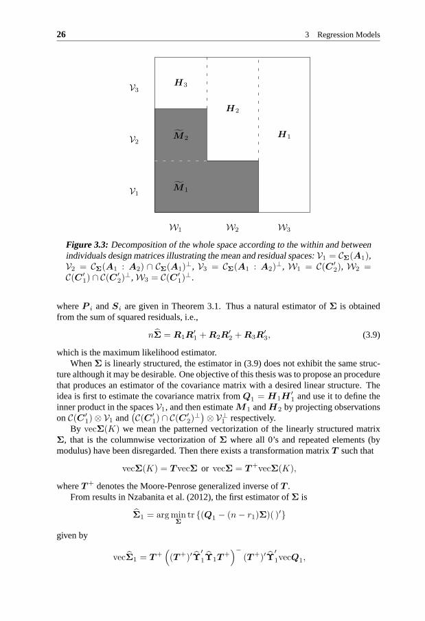
H3

Figure 3.3: Decomposition of the whole space according to the within andbetweenindividuals design matrices illustrating the mean and residual spaces:V1 = CΣ(A1),V2 = CΣ(A1 : A2) ∩ CΣ(A1)

⊥, V3 = CΣ(A1 : A2)⊥, W1 = C(C ′

2), W2 =C(C ′

1) ∩ C(C ′2)

⊥, W3 = C(C ′1)

⊥.

whereP i andSi are given in Theorem 3.1. Thus a natural estimator ofΣ is obtainedfrom the sum of squared residuals, i.e.,

nΣ = R1R′1 +R2R

′2 +R3R

′3, (3.9)

which is the maximum likelihood estimator.WhenΣ is linearly structured, the estimator in (3.9) does not exhibit the same struc-

ture although it may be desirable. One objective of this thesis was to propose an procedurethat produces an estimator of the covariance matrix with a desired linear structure. Theidea is first to estimate the covariance matrix fromQ1 = H1H

′1 and use it to define the

inner product in the spacesV1, and then estimateM1 andH2 by projecting observationsonC(C ′

1)⊗ V1 and(C(C ′

1) ∩ C(C ′2)

⊥)⊗ V⊥

1 respectively.By vecΣ(K) we mean the patterned vectorization of the linearly structured matrix

Σ, that is the columnwise vectorization ofΣ where all 0’s and repeated elements (bymodulus) have been disregarded. Then there exists a transformation matrixT such that

vecΣ(K) = T vecΣ or vecΣ = T+vecΣ(K),

whereT+ denotes the Moore-Penrose generalized inverse ofT .From results in Nzabanita et al. (2012), the first estimator of Σ is

Σ1 = argminΣ

tr (Q1 − (n− r1)Σ)( )′

given by

vecΣ1 = T+((T+)′Υ

′

1Υ1T+)−

(T+)′Υ′

1vecQ1,


whereΥ1 = (n− r1)I and the notation(Y )( )′ stands for(Y )(Y )′.

Assuming thatΣ1 is positive definite (which always holds for largen), and using itto define the inner product in the spaceV1, the estimator ofM1 andH2 are given byM1 = P

A1,Σ(s)

1

XPC′

1andH2 = (I − P

A1,Σ(s)

1

)X(PC′

1− PC′

2), respectively.

A second estimator ofΣ is obtained using the sum ofQ1 andH2H′

2 in a similar wayand is given by


′

2Υ2T+)−

(T+)′Υ′

2vecQ2,

whereQ2 = Q1+H2H′

2, Υ2 = (n−r1)I+(r1−r2)T 1⊗ T 1 andT 1 = I−PA1,Σ1

.

Assume thatΣ2 is positive definite and use it to define the inner product inV2, theestimators ofM2 andH3 are given by

M2 = PT 1A2,Σ2

XPC′

2,

H3 = T 2X(PC′

2− PC′

3),

T 2 = I − PA1,Σ1

− PT 1A2,Σ2

.

At last, a third estimator ofΣ, is obtained using the sumQ3 = Q2+H3H′

3 and is givenby


′

3Υ3T+)−

(T+)′Υ′

3vecQ3, (3.10)

whereΥ3 = (n− r1)I + (r1 − r2)T 1 ⊗ T 1 + r2T 2 ⊗ T 2.

The estimatorsΣ1, Σ2 andΣ3 are all consistent forΣ, however, asΣ3 uses all in-formation contained in all residuals, it can arguably be interpreted as a dispersion matrix.

The unbiased estimator of the mean structured is given byE[X] = M1 + M2.

Example 3.6: Example 3.5 continued

Consider again Potthoff & Roy (1964) classical dental data and the model of Example3.5. Assume that the covariance matrix has a Toeplitz structure, i.e.,

Σ(s) =

σ ρ1 ρ2 ρ3ρ1 σ ρ1 ρ2ρ2 ρ1 σ ρ1ρ3 ρ2 ρ1 σ

.

Then, the estimate of the structured covariance matrices given by (3.10) is

Σ3 =

5.2128 3.2953 3.6017 2.71463.2953 5.2128 3.2953 3.60173.6017 3.2953 5.2128 3.29532.7146 3.6017 3.2953 5.2128

.


For comparison, the MLE computed with Proc Mixed in SASr (SAS Institute Inc., 2008)is

Σ(s)

ML =

4.9368 3.0747 3.4559 2.29163.0747 4.9368 3.0747 3.45593.4559 3.0747 4.9368 3.07472.2916 3.4559 3.0747 4.9368

.

The procedures illustrated in this section were used to build up a flip-flop algorithmthat can handle the linear structuredΣ in the bilinear regression modelX ∼ Np,q(ABC,Σ,Ψ),see (Nzabanita, 2013).

3.5 Estimation in trilinear regression model

The model (3.7) can be written in matrix form using three different modes as

X(1) ∼ Np,qr(AB(1)(D ⊗C)′,Σ, Ir ⊗Ψ), (3.11)

X(2) ∼ Nq,pr(CB(2)(D ⊗A)′,Ψ, Ir ⊗Σ), (3.12)

X(3) ∼ Nr,pq(DB(3)(C ⊗A)′, Ir,Ψ⊗Σ). (3.13)

The maximum likelihood approach can be used to find estimators forB, Σ andΨ. How-ever, to find explicit estimators is not possible. Instead, we can establish estimating equa-tions that can be solved iteratively using, for example, theflip-flop algorithm. Observethat the parametersΨ andΣ are defined up to a positive multiplicative constant because,for example,Ir ⊗ cΨ⊗ c−1

Σ = Ir ⊗Ψ⊗Σ with c > 0. This issue has been discussedby some authors, among others (Dutilleul, 1999, Manceur andDutilleul, 2013, Srivastavaet al., 2008, Singull et al., 2012).

To find estimating equations for parameters we first fixΨ in (3.11) and find estimatingequations forΣ andB(1). Secondly, we fixΣ in (3.12) and find estimating equations forΨ. This procedure is justified by the fact that the models in (3.11)-(3.13) give the samelikelihood function (Nzabanita et al., 2015b). From results in Nzabanita et al. (2015b),the estimating equations for parameters in model (3.7) are given by

B(1) = (A′

S−11 A)−1

A′

S−11 X(1)(D(D′

D)−1⊗ Ψ

−1C(C′

Ψ−1

C)−1), (3.14)

S1 = X(1)(Ir ⊗ Ψ−1

−D(D′

D)−D′

⊗ Ψ−1

C(C′

Ψ−1

C)−1C

′

Ψ−1

)X ′

(1),

qrΣ = (X(1) −AB(1)(D ⊗C)′)(Ir ⊗ Ψ−1

)(X(1) −AB(1)(D ⊗C)′)′, (3.15)

prΨ = (X(2) −CB(2)(D ⊗A)′)(Ir ⊗ Σ−1

)(X(2) −CB(2)(D ⊗A)′)′, (3.16)

whereS1 is assumed to be positive definite andB(2) is obtained fromB(1) by a properrearrangement of elements.

These estimating equations are nested and cannot be solved explicitly. To obtain max-imum likelihood estimators ofΣ, Ψ andB the following iterative algorithm is proposed.

Algorithm 3.1. 1. Choose initial solutionΨ = Ψ0;

3.5 Estimation in trilinear regression model 29

2. ComputeB(1) using (3.14);

3. ComputeΣ using (3.15);

4. ComputeΨ using (3.16);

5. Repeat steps 2–4 until the convergence criterion is met.

Usually, there is no prior information that may guide to choose the initial solution.Very often the identity matrix would be enough to get the solutions. The convergencecriterion may be based on the rate of change inΨ⊗ Σ and not separately onΨ andΣ.

4Concluding Remarks

THIS chapter is reserved to the summary of contributions of this thesis and suggestionsfor further research.

4.1 Summary of contributions

In this thesis, the problem of estimating parameters in bilinear and trilinear regressionmodels has been considered. The main theme has been to propose algorithms for estimat-ing unkown parameters when the covariance matrices are structured. The main contribu-tions of the thesis are as follows:

• In Paper A, we studied the extended growth curve model with two terms and a lin-early structured covariance matrix. A simple procedure based on the decompositionof the residual space into three orthogonal subspaces and the study of the residualsobtained from projections of observations on these subspaces yielded explicit andconsistent estimators of the covariance matrix. An explicit unbiased estimator ofthe mean was also proposed.

• In Paper B, the extended generalized multivariate analysisof variance with a lin-early structured covariance matrix was considered. We showed how to decomposethe residual space, the orthogonal complement to the mean space, intom + 1 or-thogonal subspaces and how to derive explicit consistent estimators of the covari-ance matrix from the sum of squared residuals obtained by projecting observationson those subspaces. Also an explicit unbiased estimator of the mean was derived.Paper B generalizes results of Paper A.

• In Paper C, the bilinear regression models based on normallydistributed randommatrix was studied. For these models, the dispersion matrixhas the so calledKronecker product structure and they can be used for exampleto model data with

31

32 4 Concluding Remarks

spatio-temporal relationships. The aim was to estimate theparameters of the modelwhen, in addition, one covariance matrix is assumed to be linearly structured. Weproposed a flip-flop like algorithm for estimating parameters and showed that theresulting estimators are consistent.

• In Paper D, the classical growth curve model was extended to atensor versionby assuming a trilinear structure for the mean in the tensor normal model. Analgorithm for estimating model parameters was proposed.

4.2 Further research

• The algorithm proposed in Paper A & B yields estimators with good properties likeunbiasedness and/or consistency. However, to be more useful their other properties(e.g., their distributions) have to be studied. Also, more rigorous studies on thepositive definiteness of the estimates for the covariance matrix is of interest.

• The techniques used in Paper C to show the consistency of estimators can be usedto prove the consistency of other estimators based on the flip-flop algorithm.

• Paper D proposed an likelihood-based algorithm for estimating parameters in the 2-fold growth curve model. However, there is no warranty whether it produces globalsolution nor the solution does not depend on the initial guess. These issues merita deep study. Validation and other model diagnostic techniques can be developed.The model can be extended in various way, e.g., assuming different profiles (in oneor both of two growth directions) among groups. The problem of testing on themean parameters or the covariance matrix structure is of great interest.

• Finally, application of procedures developed in this thesis to concrete real data setsand a comparison with the existing ones may be useful to show their merits.

Bibliography

Allen, M. P. (1997). The origins and uses of regression analysis. In UnderstandingRegression Analysis, pages 1–5. Springer.

Anderson, T. W. (1958).An Introduction to Multivariate Statistical Analysis. Wiley, NewYork.

Basser, P. J. and Pajevic, S. (2003). A normal distribution for tensor-valued randomvariables: applications to diffusion tensor MRI.Medical Imaging, IEEE Transactionson, 22(7):785–794.

Box, G. E. P. (1950). Problems in the analysis of growth and wear curves.Biometrics,6:362–389.

De Lathauwer, L., De Moor, B., and Vandewalle, J. (2000). A multilinear singular valuedecomposition.SIAM journal on Matrix Analysis and Applications, 21(4):1253–1278.

Dutilleul, P. (1999). The MLE algorithm for the matrix normal distribution. Journal ofStatistical Computation and Simulation, 64(2):105–123.

Filipiak, K. and von Rosen, D. (2012). On MLEs in an extended multivariate lineargrowth curve model.Metrika, 75(8):1069–1092.

Fitzmaurice, G. M., Laird, N. M., and Ware, J. H. (2012).Applied Longitudinal Analysis,volume 998. John Wiley & Sons, New York.

Hoff, P. D. (2011). Separable covariance arrays via the tucker product, with applicationsto multivariate relational data.Bayesian Analysis, 6(2):179–196.

Hu, J. (2010). Properties of the explicit estimators in the extended growth curve model.Statistics, 44(5):477–492.

33

34 Bibliography

Hu, J., Yan, G., and You, J. (2011). Estimation for an additive growth curve model withorthogonal design matrices.Bernoulli, 17(4):1400–1419.

Johnson, R. A. and Wichern, D. W. (2007).Applied Multivariate Statistical Analysis.Pearson Education International, New York.

Kattan, W. M. and Gönen, M. (2008). The prediction philosophy in statistics.UrologicOncology: Seminars and Original Investigations, 26(3):316–319.

Khatri, C. G. (1966). A note on a MANOVA model applied to problems in growth curve.Annals of the Institute of Statistical Mathematics, 18(1):75–86.

Khatri, C. G. (1973). Testing some covariance structures under a growth curve model.Journal of Multivariate Analysis, 3(1):102–116.

Klein, D. and Žežula, I. (2009). The maximum likelihood estimators in the growth curvemodel with serial covariance structure.Journal of Statistical Planning and Inference,139(9):3270–3276.

Kolda, T. G. and Bader, B. W. (2009). Tensor decompositions and applications.SIAMreview, 51(3):455–500.

Kollo, T. and von Rosen, D. (2005).Advanced Multivariate Statistics with Matrices.Springer, Dordrecht.

Lange, N. and Laird, N. M. (1989). The effect of covariance structure on variance es-timation in balanced growth-curve models with random parameters. Journal of theAmerican Statistical Association, 84(405):241–247.

Lee, J. C. (1988). Prediction and estimation of growth curves with special covariancestructures.Journal of the American Statistical Association, 83(402):432–440.

Lee, J. C.-S. and Geisser, S. (1975). Applications of growthcurve prediction.Sankhya:The Indian Journal of Statistics, Series A, 37(2):239–256.

Lu, N. and Zimmerman, D. L. (2005). The likelihood ratio testfor a separable covariancematrix. Statistics and Probability Letters, 73(4):449–457.

Manceur, A. M. and Dutilleul, P. (2013). Maximum likelihoodestimation for the tensornormal distribution: Algorithm, minimum sample size, and empirical bias and disper-sion. Journal of Computational and Applied Mathematics, 239:37–49.

Nzabanita, J. (2013). Multivariate linear models with kronecker product and linear struc-tures on the covariance matrices. InProceedings, JSM 2013-IMS, pages 1582–1588.Alexandria, VA: American Statistical Association.

Nzabanita, J., Singull, M., and von Rosen, D. (2012). Estimation of parameters in theextended growth curve model with a linearly structured covariance matrix. Acta etCommentationes Universitatis Tartuensis de Mathematica, 16(1):13–32.

Bibliography 35

Nzabanita, J., von Rosen, D., and Singull, M. (2015a). Extended GMANOVA modelwith a linearly structured covariance matrix.Linköping University Electronic Press,LiTH-MAT-R-2015/07-SE.

Nzabanita, J., von Rosen, D., and Singull, M. (2015b). Maximum likelihood estimationin the tensor normal model with a structured mean.Linköping University ElectronicPress, LiTH-MAT-R-2015/08-SE.

Ohlson, M., Ahmad, M. R., and von Rosen, D. (2013). The multilinear normal dis-tribution: Introduction and some basic properties.Journal of Multivariate Analysis,113:37–47.

Ohlson, M., Andrushchenko, Z., and von Rosen, D. (2011). Explicit estimators under m-dependence for a multivariate normal distribution.Annals of the Institute of StatisticalMathematics, 63(1):29–42.

Ohlson, M. and von Rosen, D. (2010). Explicit estimators of parameters in the growthcurve model with linearly structured covariance matrices.Journal of Multivariate Anal-ysis, 101(5):1284–1295.

Olkin, I. and Press, S. G. (1969). Testing and estimation fora circular stationary model.The Annals of Mathematical Statistics, 40(4):1358–1373.

Pothoff, R. F. and Roy, S. N. (1964). A generalized multivariate analysis of variancemodel useful especially for growth curve problems.Biometrika, 51:313–326.

Rao, C. R. (1958). Some statistical methods for comparison of growth curves.Biometrics,14(1):1–17.

Rao, C. R. (1965). The theory of least squares when the parameters are stochastic and itsapplication to the analysis of growth curves.Biometrika, 52:447–458.

Rao, C. R. and Toutenburg, H. (1995).Linear Models. Springer-Verlang, New York.

Roy, A. and Khattree, R. (2005). On implementation of a test for Kronecker productcovariance structure for multivariate repeated measures data. Statistical Methodology,2(4):297–306.

Roy, S. N. (1957).Some Aspects of Multivariate Analysis. Wiley, New York.

SAS Institute Inc. (2008).SAS/STATr 9.2 User’s Guide: The MIXED Procedure (BookExcerpt). Cary, NC: SAS Institute Inc.

Singull, M., Ahmad, M. R., and von Rosen, D. (2012). More on the Kronecker struc-tured covariance matrix.Communications in Statistics-Theory and Methods, 41(13-14):2512–2523.

Srivastava, M. S. and Khatri, C. G. (1979).An Introduction to Multivariate Statistics.North-Holland, New York, USA.

36 Bibliography

Srivastava, M. S. and Singull, M. (2015). Testing some covariance structures under agrowth curve model in high dimension.Linköping University Electronic Press, LiTH-MAT-R–2015/03.

Srivastava, M. S., von Rosen, T., and von Rosen, D. (2008). Models with a Kroneckerproduct covariance structure: estimation and testing.Mathematical Methods of Statis-tics, 17(4):357–370.

Szatrowski, T. H. (1982). Testing and estimation in the block compound symmetry prob-lem. Journal of Educational Statistics, 7(1):3–18.

Tucker, L. R. (1964). The extension of factor analysis to three-dimensional matrices.Contributions to mathematical psychology, pages 109–127.

Verbyla, A. P. and Venables, W. N. (1988). An extension of thegrowth curve model.Biometrika, 75(1):129–138.

von Rosen, D. (1989). Maximum likelihood estimators in multivariate linear normalmodels.Journal of Multivariate Analysis, 31(2):187–200.

Votaw, D. F. (1948). Testing compound symmetry in a normal multivariate distribution.The Annals of Mathematical Statistics, 19(4):447–473.

Wilks, S. S. (1946). Sample criteria for testing equality ofmeans, equality of variances,and equality of covariances in a normal multivariate distribution. The Annals of Math-ematical Statistics, 17(3):257–281.

Wishart, J. (1928). The generalized product moment distribution in samples from a nor-mal multivariate population.Biometrika, 20(A):32–52.

Part II

Papers

37

Papers

The articles associated with this thesis have been removed for copyright reasons. For more details about these see: http://urn.kb.se/resolve?urn=urn:nbn:se:liu:diva-118089

http://urn.kb.se/resolve?urn=urn:nbn:se:liu:diva-118089

Documents

Bilinear and Trilinear Regression Models with Structured ...liu.diva-portal.org/smash/get/diva2:813054/FULLTEXT01.pdf · Models with Structured Covariance Matrices ... Alexandre Lyambabaje,