Bilevel Integer Programming - Lehigh University

Bilevel Integer Programming

Ted Ralphs1

Joint work with:Scott DeNegre1, Menal Guzelsoy2,

Andrea Lodi3, Fabrizio Rossi4, Stefano Smriglio4

1COR@L Lab, Department of Industrial and Systems Engineering, Lehigh University2ISyE, Georgia Institute of Technology

3DEIS, Universitá di Bologna4Dipartimento di Informatica, Universitá di L’Aquila

Ralphs, et al. (COR@L Lab) BILP Aussois, January 2009 1 / 40

Outline

1 IntroductionMotivationSetup

2 ApplicationsPracticalTheoretical

3 AlgorithmsRecourse ProblemsContinuous BLPsDiscrete BLPs

4 Implementation


Motivation

A standard mathematical program models a set of decisions tobe madesimultaneouslyby asingledecision-maker (i.e., with asingleobjective).

Many decision problems arising both in real-world applications and in the theoryof integer programming involve

multiple, independent decision-makers(DMs),multiple, possibly conflicting objectives, and/orhierarchical/multi-stage decisions.

Modeling frameworksMultiobjective Programming⇐ multiple objectives, single DMMathematical Programming with Recourse⇐ multiple stages, single DMMultilevel Programming⇐ multiple stages, multiple DMs

Multilevel programminggeneralizes standard mathematical programming bymodeling hierarchical decision problems, such as Stackelberg games.

Such models arises in aremarkably wide array of applications.


Bilevel (Integer) Linear Programming

Formally, abilevel linear programis described as follows.

x ∈ X ⊆ Rn1 are theupper-level variables

y ∈ Y ⊆ Rn2 are thelower-level variables

Bilevel (Integer) Linear Program

max

c1x + d1y | x ∈ PU ∩ X, y ∈ argmind2y | y ∈ PL(x) ∩ Y

(MIBLP)

Theupper-andlower-level feasible regionsare:

PU =

x ∈ R+ | A1x ≤ b1

and

PL(x) =

y ∈ R+ | G2y ≥ b2 − A2x

.

For most of the talk, we assumeX = Zn1 andY = Zn2.


Notation

Notation

ΩI = (x, y) ∈ (X × Y) | x ∈ PU, y ∈ SL(x)

Ω = (x, y) ∈ (Rn1 × Rn2) | x ∈ PU, y ∈ SL(x)

MI (x) = argmind2y | y ∈ (PL(x) ∩ Y)

F I =

(x, y) | x ∈ (PU ∩ X), y ∈ MI (x)

F =

(x, y) | x ∈ PU, y ∈ argmind2y | y ∈ SL(x)

Underlying bilevel linear program (BLP):

min(x,y)∈F

c1x + d1y

Underlying MILP:min

(x,y)∈ΩIc1x + d1y

Underlying LP:min

(x,y)∈Ωc1x + d1y


Applications

Hierarchical decision systemsGovernment agenciesLarge corporations with multiple subsidiariesMarkets with a single “market-maker.”Decision problems with recourse

Parties in direct conflictZero sum gamesInterdiction problems

Modeling “robustness”: leader represents external phenomena that cannot becontrolled.

WeatherExternal market conditions

Controlling optimized systems: follower represents a system that is optimized byits nature.

Electrical networksBiological systems


Bilevel Structure in Branch and Cut

We consider aninteger program(IP) of the form

minc⊤x | x ∈ P ∩ Zn, (1)

whereP = x ∈ Rn+ | Ax≥ b, A ∈ Qm×n, b ∈ Qm, c ∈ Qn.

A branch-and-cut algorithmto solve this problem requires the solution of twofundamental decision problems.

Definition 1 Theseparation problemfor a polyhedronQ is to determine for agivenx ∈ Rn whether or notx ∈ Q and if not, to produce an inequality(α, β) ∈ Rn+1 valid forQ and for whichα⊤x < β.

Definition 2 Thebranching problemfor a setS is to determine for a givenx ∈ Rn whetherx ∈ S and if not, to produce a disjunction

∨

h∈Q

Ahx ≥ bh, x ∈ S (2)

that is satisfied by all points inS, but not satisfied byx.


Bilevel Structure of the Separation Problem

Often, we wish to select an inequality thatmaximizes violation, i.e.,

(α, β) ∈ argmin(α,β)∈Rn+1α⊤x− β | α⊤x ≥ β ∀x ∈ Q (3)

To make the problem tractable, we may restrict ourselves to aspecifictemplateclassof valid inequalities with well-defined structure.

Given a classC, calculation of the right-hand sideβ required to ensure(α, β) is amember ofC may itself be an optimization problem.

The separation problem for the classC with respect to a givenx ∈ Rn can then inprinciple be formulated as the bilevel program:

min α⊤x− β (4)

α ∈ Cα (5)

β = minα⊤x | x ∈ F, (6)

where the setCα ⊆ Rn is the projection ofC into the space of coefficient vectorsandF is the closure over the classC.


Example: Disjunctive cuts

Given a MIP in the form (1), Balas (1979) showed how to derive avalidinequality by exploiting any fixed disjunction

π⊤x ≤ π0 OR π⊤x ≥ π0 + 1 ∀x ∈ Rn, (7)

whereπ ∈ Zn andπ0 ∈ Z.

A disjunctive inequalityis one valid for the convex hull of union ofP1 andP2,obtained by imposing the two terms of the disjunction.

Conceptually, theseparation problemcan be written as the followingbilevelprogram:

min α⊤x− β (8)

α ≥ u⊤A− uoπ (9)

α ≥ v⊤A + voπ (10)

u, v, u0, v0 ≥ 0 (11)

u0 + v0 = 1 (12)

β = minα⊤x | x ∈ P1 ∪ P2 (13)


Example: Disjunctive Cuts (cont.d)

Equation (13) requiresβ to have the largest value consistent with validity.

To ensure the cut is valid, we need only ensure that

β ≤ minu⊤b− u0π0, v⊤b + v0(π0 + 1). (14)

Using the standard modeling trick, we can rewrite (14) as

β ≤ u⊤b− u0π0 (15)

β ≤ v⊤b + v0(π0 + 1). (16)

The sense of the optimization ensures that (14) holds at equality.


Example: Capacity Constraints for CVRP

In the Capacitated Vehicle Routing Problem (CVRP), thecapacity constraintsare of the form

∑

e=i,j∈Ei∈S,j 6∈S

xe ≥ 2b(S) ∀S⊂ N, |S| > 1, (17)

whereb(S) is any lower boundon the number of vehicles required to servecustomers in setS.By definingbinary variables

yi = 1 if customeri belongs toS, andze = 1 if edgee belongs toδ(S),

we obtain the following bilevel formulation for the separation problem:

min∑

e∈E

xeze − 2b(S) (18)

ze ≥ yi − yj ∀e∈ E (19)

ze ≥ yj − yi ∀e∈ E (20)

b(S) = maxS | b(S) is a valid lower bound (21)


Example: Capacity Constraints for CVRP (cont.d)

If the bin packing problem is used in the lower-level, the formulation becomes:

min∑

e∈E

xeze − 2b(S) (22)

ze ≥ yi − yj ∀e = i, j (23)

ze ≥ yj − yi ∀e = i, j (24)

b(S) = minn

∑

ℓ=1

hℓ (25)

n∑

ℓ=1

wℓi = yi ∀i ∈ N (26)

∑

i∈N

diwℓi ≤ Khℓ ℓ = 1, . . . , n, (27)

where we introduce the additional binary variables

wℓi = 1 if customeri is served by vehicleℓ, and

hℓ = 1 if vehicleℓ is used.Ralphs, et al. (COR@L Lab) BILP Aussois, January 2009 12 / 40

Bilevel Structure of the Branching Problem

A typical criteria for selecting a branching disjunction isto maximize the boundincrease resulting from imposing the disjunction.

The problem of selecting the disjunction whose imposition results in the largestbound improvement has a naturalbilevel structure.

The upper-level variables can be used to model thechoice of disjunction(we’ll seean example shortly).The lower-level problem models thebound computationafter the disjunction hasbeen imposed.

In strong branching, we are solving this problem essentially by enumeration.

The bilevel branching paradigm is to select the branching disjunction directly bysolving abilevel program.


Example: Interdiction Branching

The following is a bilevel programming formulation for the problem of finding asmallest branching set in interdiction branching:

(BBP) max∑

c⊤xs.t.

c⊤x ≤ z

y ∈ Bn

x ∈ arg maxx c⊤xs.t.

xi + yi ≤ 1, i ∈ Na

x ∈ Fa

whereF is the feasible region of a given relaxation of the original problem used forcomputing the bound.


Algorithms: Technical Assumptions

We make the following assumptions to simplify and ensure theproblem has asolution.

Assumptions

1 For every action by the leader, the follower has a rational reaction(PL(x) ∩ Y 6= ∅ for all x ∈ PU ∩ X).

2 The follower is semi-cooperative (the leader may choose amongalternative members ofMI (x)).

3 The feasible setF I is nonempty and compact.


Back to the Example

Consider again the following instance of (MIBLP) from Mooreand Bard (1990).

minx∈Z

− x − 10y

subject to y ∈ argminy : 25x − 20y ≥ −30

−x − 2y ≥ −10

−2x + y ≥ −15

2x + 10y ≥ 15

y ∈ Z

8

1

2

3

4

5

1 2 3 4 5 6 7

conv(F I)

F

conv(ΩI)

x

y

F I

From the figure, we can make several observations:1 F ⊆ Ω, F I ⊆ ΩI , andΩI ∈ Ω

2 FI 6⊆ F

3 Solutions to (MIBLP) do not occur at extreme points ofconv(ΩI )


Properties of MIBLPs

In this example:

Optimizing overF yields theintegersolution(8, 1), with the upper-levelobjective value18.

Imposing integrality yields the solution(2, 2), with upper-level objective value22

From this we can make two important observations:

1 The objective value obtained by relaxing integrality is nota valid boundon the solution value of the original problem,

2 Even when solutions tomax(x,y)∈F c1x + d1y are inF I , they are notnecessarily optimal.

Thus, some familiar properties from the MILP case do not holdhere.


Special Case: Recourse Problems

If d1 = −d2, we can view this as amathematical program with recourse.Two-stage stochastic programs with recourse are a special case (under mildconditions).The resulting problem can be solved as a standard mathematical program.For the case whenY = Rn, we can solve the problem by Benders Decomposition.Note that the value function of the lower-level problem is convex in theupper-level variables, so we can also reformulate as a convex programThis is a useful way of visualizing the situation.

zLP (b) + u∗(v − b)

zLP

v

b


Special Case: Continuous BLPs

In the continuous case, the lower-level problem can be replaced with itsoptimality conditions.

The optimality conditions for the lower-level optimization problem are

G2y ≥ b2 − A2x

uG2 ≤ d2

u(b2 − G2 − A2x) = 0

(d2 − uG2)y = 0

u, y ∈ R+

Note that this is a special case of a class of non-linear mathematical programsknown asmathematical programs with equilibrium constraints(MPECs).

This can be solved in a number of ways, including converting it to standardinteger program.

Note that in this case, the value function of the lower-levelproblem is piecewiselinear, but not necessarily convex.


General Case: Discrete BLPs

When some/all of the variables are discrete, the situation is a bit more difficult.

Because the duals that exist for general integer programs are not tractable ingeneral, we cannot use the same approach as we did for the continuous case.

In fact, going from the continuous case to the discrete case in the bilevel settingposes significantly different challenges than for standardMILPs.

Nevertheless, we have developed abranch-and-cut algorithmthat attempts togeneralize techniques from MILP.


Lower Bounds

Relaxing integrality conditionsandthe requirementy ∈ MI (x) yields the relaxation

max(x,y)∈Ω

c1x + d1y. (LR)

The resulting bound can be used in combination with a standard variablebranching scheme to yield an algorithm that solves (MIBLP).

Unfortunately, the bound is too weak to be effective on interesting problems.

As usual, we strengthen the linear relaxation by exploitingdisjunctions valid forthe bilevel feasible region.


Valid Disjunctions for MIBLP

Bilevel Feasibility Conditions

1 (x, y) ∈ Ω ,2 (x, y) ∈ X × Y , and3 y ∈ MI (x).

To develop a successful branch-and-cut algorithm, we wouldlike to derivedisjunctions arising from violation of these conditions.

Violations of Conditions 1 and 2 can be dealt with as in the MILP case.

Violations of Condition 3 are both difficult to detect in general and difficult toexploit.


Bilevel Feasibility Check

Let (x, y) be a solution to LR.

We fix x = x and solve the lower-level problem

miny∈P I

L(x)d2y (28)

with the fixed upper-level solutionx.

Let y∗ be the solution to (28).

(x, y∗) is bilevel feasible⇒ c1x + d1y∗ is a valid upper bound on the optimal valueof the original MIBLP

Either1 d2y = d2y∗ ⇒ (x, y) is bilevel feasible.2 d2y > d2y∗ ⇒ generate a valid inequality violated by(x, y).


Bilevel Feasibility Cut (Pure Integer Case)

Let

A :=

[

A1

A2

]

, G :=

[

0G2

]

, and b :=

[

b1

b2

]

.

A basic feasible solution(x, y) ∈ ΩI to (LR) is theuniquesolution to

a′i x + g′i y = bi, i ∈ I

whereI is the set of active constraints at(x, y).

This implies that

(x, y) ∈ ΩI |∑

i∈I

a′i x + g′i y =∑

i∈I

bi

=

(x, y)

and∑

i∈I a′i x + g′i y ≤∑

i∈I bi is valid forΩ.


Bilevel Feasibility Cut (cont.)

A Valid Inequality∑

i∈I a′i x + g′i y ≤∑

i∈I bi − 1 is valid forΩI \ (x, y).

maxx

miny

y | −x + y ≤ 2,−2x− y ≤ −2, 3x− y ≤ 3, y ≤ 3, x, y ∈ Z+ .

1 2 3

2

3

1

x

y

−x + 2y ≤ 5

−x + 2y ≤ 4

This yields a finite algorithm in the pure integer case.


Exploiting the Value Function

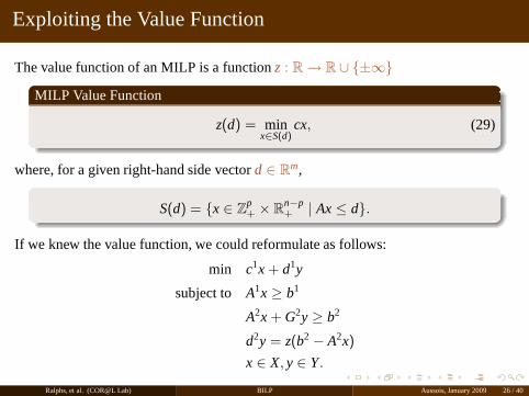
The value function of an MILP is a functionz : R → R ∪ ±∞

MILP Value Function

z(d) = minx∈S(d)

cx, (29)

where, for a given right-hand side vectord ∈ Rm,

S(d) = x ∈ Zp+ × R

n−p+ | Ax≤ d.

If we knew the value function, we could reformulate as follows:

min c1x + d1y

subject to A1x ≥ b1

A2x + G2y ≥ b2

d2y = z(b2 − A2x)

x ∈ X, y ∈ Y.


Example

min 3x1 + 72x2 + 3x3 + 6x4 + 7x5 + 5x6

s.t 6x1 + 5x2 − 4x3 + 2x4 − 7x5 + x6 = b andx1, x2, x3 ∈ Z+, x4, x5, x6 ∈ R+.

(SP)

0 2 4 6 8 10 12 14 16 18 20 22 24 26 28-2-4-6-8-10-12-14-16

2

4

6

8

10

12

14

16

18

d

z


Bounding the Value Function

To generate valid disjunctions violated by solutions not satisfying Condition 3, wemust somehow bound the value function.

Upper boundscan be derived by considering the value function ofrestrictionsofthe original problem.⇒ Fix some integer variables.

Lower boundscan be derived by considering the value function ofrelaxationsofthe original problem.⇒ Relax integrality of some variables.

Lower boundscan also be obtained by considering so-calleddual functionsthatcan be constructed in a number of ways.


Upper Bound (Single Constraint Case)

0d

d∗

f(d∗, ηC)

f(d∗, ζC)

For anyd ≤ d∗,

z(d) ≤ maxf (d∗, ζC), f (d∗, ηC) = f (d∗, ζC).

Similarly, for anyd ≥ d∗,

z(d) ≤ maxf (d∗, ζC), f (d∗, ηC) = f (d∗, ηC).


Bilevel Feasibility Disjunctions (Single Constraint Case)

Thus, we have the following disjunction.

Bilevel Feasibility Disjunction

b2 − A2x ≤ b2 − A2x AND d2y ≤ f (b2 − A2x, ζC)

OR

b2 − A2x ≥ b2 − A2x AND d2y ≤ f (b2 − A2x, ηC).

Such a disjunction can be used to eitherbranchor cutwhen solutions(x, y) ∈ ΩI suchthaty 6∈ MI (x) are found.


Numerical Example (Disjunctive Cut)

MIBLP Example

min 8x1 + x2 + 2x3 + 3x5 + 4x6

+ y1 + 3y2 + 2y3 + 4y4 + 2y6

subject to 4x1 + 2x2 − 4x3 + 3x4 + 6x5 + x6 = 24

x1, x2, x3 ∈ Z+, x4, x5, x6 ∈ R+

y ∈ argmin 2y1 + 2y3 + 8y4 + 4y5 + 3y6 :

2x1 − x2 + 4x3 − 4x4 + 3x5 + x6

+ 4y1 − 6y2 + 6y3 + 4y4 − 4y5 +43

y6 = 16,

y1, y2, y3 ∈ Z+, y3, y5, y6 ∈ R+ ,


Numerical Example (cont.)

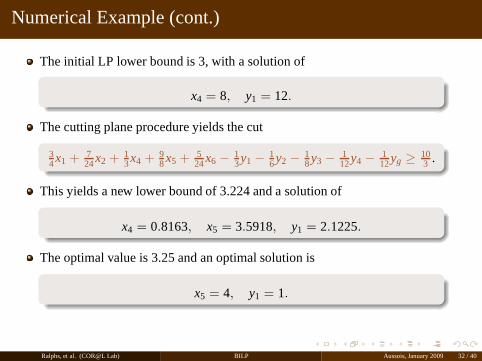
The initial LP lower bound is 3, with a solution of

x4 = 8, y1 = 12.

The cutting plane procedure yields the cut

34x1 + 7

24x2 + 13x4 + 9

8x5 + 524x6 −

13y1 −

16y2 −

18y3 −

112y4 −

112yg ≥ 10

3 .

This yields a new lower bound of 3.224 and a solution of

x4 = 0.8163, x5 = 3.5918, y1 = 2.1225.

The optimal value is 3.25 and an optimal solution is

x5 = 4, y1 = 1.


Jeroslow Formula for General MILP

Let the setE consist of the index sets of dual feasible bases of the linearprogram

min1M

cCxC :1M

ACxC = b, x ≥ 0

whereM ∈ Z+ such that for anyE ∈ E, MA−1E aj ∈ Zm for all j ∈ I .

Theorem 1 (Jeroslow Formula) There is ag ∈ G m such that

z(d) = minE∈E

g(⌊d⌋E) + vE(d − ⌊d⌋E) ∀d ∈ Rm with S(d) 6= ∅,

where forE ∈ E, ⌊d⌋E = AE⌊A−1E d⌋ andvE is the corresponding basic feasible

solution.


Generalizing

The question of how to derive practical disjunctions based on local structure inthe general case is still largely unanswered.

The Jeroslow formula (among others) tells us what the local structure looks like.

We can derive local structure from the branch-and-bound tree constructed whenwe do the bilevel feasibility check.

There is an obvious combinatorial explosion.


Implementation

The Mixed Integer Bilevel Solver (MibS) implements the branch and boundframework described here using software available from theComputationalInfrastructure for Operations Research (COIN-OR) repository.

COIN-OR Components Used

TheCOIN High Performance Parallel Search(CHiPPS) framework toperform the branch and bound.

TheCOIN Branch and Cut(CBC) framework for solving the MILPs.

TheCOIN LP Solver(CLP) framework for solving the LPs arising in thebranch and cut.

TheCut Generation Library(CGL) for generating cutting planes withinCBC.

TheOpen Solver Interface(OSI) for interfacing with CBC and CLP.


What Is Implemented

MibS is still in its infancy and is not fully general. Currently, we have:

Bilevel feasibility cuts(pure integer case).

Specialized methods (primarily cuts) forpure binary at the upper level.

Specialized methods forinterdiction problems.

Disjunctive cutsbased on the value function for lower-level problems with asingle constraint.

Severalprimal heuristics.

Simplepreprocessing.


Preliminary Results from Knapsack Interdiction

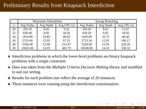
Maximum Infeasibility Strong Branching2n Avg Nodes Avg Depth Avg CPU (s) Avg Nodes Avg Depth Avg CPU (s)20 359.30 8.65 9.32 358.30 8.65 11.0722 658.40 9.85 18.50 658.20 9.85 18.9224 1414.80 10.85 46.03 1410.80 10.75 46.4626 2725.00 12.05 97.55 2723.50 12.05 100.1728 5326.40 12.90 214.97 5328.60 12.95 220.2630 10625.00 14.05 482.70 10638.00 14.10 538.32

Interdiction problems in which the lower-level problems are binary knapsackproblems with a single constraint.

Data was taken from theMultiple Criteria Decision Makinglibrary and modifiedto suit our setting.

Results for each problem size reflect the average of 20 instances.

These instances were running using the interdiction customization.


Preliminary Results from Assignment Interdiction

Instance Nodes Depth CPU (s)2AP05-1 6203 33 290.252AP05-2 3881 32 384.972AP05-3 3909 32 205.932AP05-4 2441 36 102.662AP05-5 3505 33 119.182AP05-6 2031 35 80.312AP05-7 2957 29 153.022AP05-8 3549 32 224.772AP05-9 2271 33 111.132AP05-10 3299 31 211.072AP05-11 707 33 35.132AP05-12 407 18 29.512AP05-13 391 18 23.802AP05-14 3173 28 261.082AP05-15 2509 32 127.052AP05-16 1699 29 44.612AP05-17 5417 29 201.342AP05-18 5785 32 176.672AP05-19 2259 32 79.702AP05-20 2585 31 77.352AP05-21 6039 33 161.442AP05-22 2479 29 48.062AP05-23 1519 25 49.402AP05-24 15 5 1.322AP05-25 3857 31 115.97

Here, the lower-level problems are binary assignment problems.

Data also taken fromMultiple Criteria Decision Makinglibrary.

Problems have 50 variables and 45 constraints.


Conclusions and Future Work

Preliminary testing to date has revealed that these problems can be extremelydifficult to solve in practice.

What we have implemented so far has only scratched the surface.

Currently, we are focusing on special cases where we can get traction.Interdiction problemsStochastic integer programs

Much work remains to be done.

Please join us!


References I

Balas, E. 1979. Disjunctive programming.Annals of Discrete Mathematics5, 3–51.

Moore, J. and J. Bard 1990. The mixed integer linear bilevel programming problem.Operations Research38(5), 911–921.


Documents

Bilevel Integer Programming - Lehigh University