Bifurcation Analysis for Time Steppers

Laurette Tuckerman

laurette@pmmh.espci.fr

THE THREE TOOLS OF

COMPUTATIONAL FLUID DYNAMICS

Time stepping: ∂tU = LU +N(U)

Steady state solving: 0 = LU +N(U)

Linear stability analysis: λu = Lu+NUu

Heat Equation

∂tu = ∂2xxu

u(x, t) =

kmax∑

k=1

uk(t) sin kx

∂tuk = −k2uk

EXACT SOLUTION

uk(t+ ∆t) = e−k2∆tuk(t)

EXPLICIT EULER

uk(t+ ∆t) = uk(t)− k2∆tuk(t)

= (1− k2∆t)uk(t)

As kmax →∞, ∆tmax = 2k2max

→ 0

IMPLICIT EULER

uk(t+ ∆t) = uk(t)− k2∆tuk(t+ ∆t)

(1 + k2∆t)uk(t+ ∆t) = uk(t)

uk(t+ ∆t) = (1 + k2∆t)−1uk(t)

Matrix version:

u(t+ ∆t) = (I −∆tL)−1u(t)

NAVIER-STOKES EQUATIONS

∂tU = −(U · ∇)U −∇P + ν∇2U

= −(I −∇∇−2∇·)(U · ∇)U + ν∇2U

= N(U) + L U

• Time stepping (Direct Numerical Simulation)

∂tU = N(U) + L U ≡ A(U)

Explicit/Implicit Euler:

U(t+ ∆t) = U(t) + ∆t[N(U(t)) + LU(t+ ∆t)]

= (I −∆tL)−1(I + ∆tN)U(t) ≡ BU(t)

• Steady state solving

0 = N(U) + L U

Newton’s method:

{AUu = A(U)

U ← U − u

• Linear stability analysis:

λu = NU u+ L u ≡ AUu

Arnoldi/block power method:

un+1 = A−1U un or un+1 = eAU∆tun

NUu ≡ −(U · ∇)u− (u · ∇)U

AUu = NUu+ Lu

STEADY STATE SOLVING

0 = F (U)

Newton’s method

0 = F (U − u) ≈ F (U)−DF (U)u{DF (U)u = F (U)

U ← U − u

Need to solve:

(NU + L)u = s

where u could be a 3D field of size

3× 100× 100× 100 = 3× 106

Q: When are matrix operations cheap?

A: When the matrix is structured, e.g. tensor product.

Example: Fourier Transform

[Fx Fy Fz] U(x, y, z) = U(kx, ky, kz)

Operation count:

MxMyMz (Mx +My +Mz)≪ (MxMyMz)2

Actually even less:

MxMyMz (logMx + logMy + logMz)

Poisson (or Helmholtz) equation:

s(x, y) =(

∂2x + ∂2

y

)

p(x, y)

=(

ExΛ2xE−1x + EyΛ

2yE−1y

)

p(x, y)

= (ExEy)(

Λ2x + Λ2

y

)

(ExEy)−1p(x, y)

because Ex, Ey commute.

Operation count:

MxMy (Mx +My)→MxMyMz (Mx +My +Mz)

Exponential (integration of heat equation):

U(x, y, t+ ∆t) = exp(

∆t(∂2x + ∂2

y))

U(x, y, t)

= (ExEy) exp(

∆t(Λ2x + Λ2

y))

(ExEy)−1U(x, y, t)

Acting with ∇2 or ∇−2 or exp(∆t∇2) is inexpensive in a

tensor-product grid for spectral or finite-difference methods.

Finite element and spectral element methods have their own

tricks for fast direct action/inversion.

(Static condensation? Schur complement?)

Applies to∇2 = L, not full Jacobian.

Used for implicit time-integration of diffusive/viscous step.

How to solve linear systems?

1) Direct: Gaussian Elimination = LU + Backsolve

Storage: M2 Time: M3

For 3D case withMx = My = Mz = 102, we haveM = 106

M2 = 1012 M3 = 1018

2) Iterative: Conjugate Gradient methods

Use only matrix-vector products u→ Au

For an arbitrary matrix,

Each product u→ Au requiresM2 operations

Convergence requiresM iterations

}

M3

Can gain:

IfA is structured or sparse, then u→ Au takes∼M ops

IfA is well-conditioned, convergence takes few iterations.

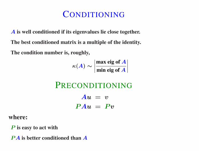
CONDITIONING

A is well conditioned if its eigenvalues lie close together.

The best conditioned matrix is a multiple of the identity.

The condition number is, roughly,

κ(A) ∼

∣∣∣∣

max eig ofA

min eig ofA

∣∣∣∣

PRECONDITIONING

Au = v

PAu = Pv

where:

P is easy to act with

PA is better conditioned thanA

Extreme cases:

P = I (easy to act with but no improvement)

P = A−1 (perfect preconditioner but impossible)

Our case:

AUu = Lu+NUu

For 3D case withMx = My = Mz = 100,

eigs of L range from∼ −1 to−(M2x +M2

y +M2z ) = −30000.

Idea:

L is the main source of difficulty =⇒ Use P = L−1

Question: Where do we get L−1?

Answer: Already present in a timestepping code!

U(t+ ∆t)− U(t) =[(I −∆tL)−1(I + ∆tN)− I

]U(t)

= (I −∆tL)−1 [I + ∆tN − (I −∆tL)]U(t)

= (I −∆tL)−1∆t(N + L) U(t)

(B − I)U(t) ≡ U(t+ ∆t)− U(t) has same roots as (N + L)!

• In time-stepping, ∆t must be small (∼ 10−2) to insure

(I −∆tL)−1(1 + ∆tNU) ≈ exp((L+NU)∆t).

• Here, ∆t plays algebraic role, and can (should) be large (& 102).

•∆t interpolates between P = I and P = L−1.

• Called Stokes preconditioning

ONE NEWTON STEP

(I −∆tL)−1∆t(NU + L) u = (I −∆tL)−1∆t(N + L) U

[(I −∆tL)−1(I + ∆tNU)− I

]u

︸ ︷︷ ︸=

[(I −∆tL)−1(I + ∆tN)− I

]U

︸ ︷︷ ︸

difference between two difference between two

widely spaced consecutive widely spaced consecutive

linearized timesteps timesteps

Solve linear system with BI-CGSTAB

H.A. van der Vorst, Bi-CGSTAB: A fast and smoothly converging variant of

Bi-CG for the solution of nonsymmetric linear systems, SIAM J. Sci. Stat.

Comput. 13, 631 (1992)

∼ 30 lines of code

CONTINUATION

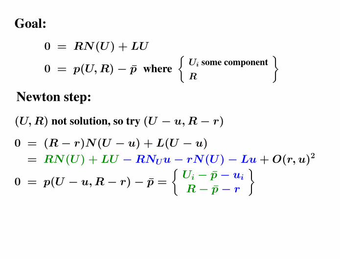
Goal:

0 = RN(U) + LU

0 = p(U,R)− p where

{Ui some component

R

}

Newton step:

(U,R) not solution, so try (U − u,R− r)

0 = (R− r)N(U − u) + L(U − u)

= RN(U) + LU −RNUu− rN(U)− Lu+ O(r, u)2

0 = p(U − u,R− r)− p =

{Ui − p− uiR− p− r

}

[RNU + L N(U)

0 0 . . . 0 1 0 . . . 0 1

]

︸ ︷︷ ︸

[u

r

]

=

RN(U) + LU{Ui − p

R− p

}

or

If p(U,R) = R (i.e. set Reynolds number),

then setR = p, r = 0 and get previous case:

L−1 [RNU + L] [u] = L−1 [RN(U) + LU ]

If p(U,R) = Ui, then must solve extended system for (u, r).

[L−1(RNu + L) L−1N(U)

0 0 . . . 0 1 0 . . . 0 0

] [u

r

]

=

[L−1(RN(U) + LU)

Ui − p

]

Set ui = Ui − p

Calculate L−1(RNU + L)u

Add L−1N(U)r

Use only vectors and

operators of lengthM

TRAVELING WAVES: U(x− Ct, y, z)

Goal :

{0 = C∂xU +N(U) + LU

0 = p(U)− p

[C∂x +NU + L ∂xU

0 0 . . . 0 1 0 . . . 0 0

] [u

c

]

=

[C∂xU +N(U) + LU

Ui − p

]

Extreme Multiplicity in CylindricalRayleigh-Benard Convection

with K. Boronska

Hof, Lucas & Mullin, Phys. Fluids (1999)

Results from Time-Dependent Simulations

���������� ������ ������

Ra

��

�������

������

������

��� ����

�����

����������

������

�����

�����

�������

������������

two-tori torus

mercedes four rolls

pizza dipole

two rolls three rolls

CO asym three rolls

(U, V,W, T ) = 4×Nr ×Nθ ×Nz = 4× 40× 120× 20 = 384 000

Complete Bifurcation Diagram

Thresholds from Conductive State

m = 1 m = 2 m = 0 m = 3

Pizza: Bifurcations fromm = 2 mode

Conductive|

1849 1879 2353 22 660

..

..

..

..

..

..

..

..

..

..

.

..

..

..

..

..

..

..

..

..

..

.

..

..

..

..

..

..

..

..

..

..

..

..

..

..

..

..

..

..

..

..

..

Pizza

.

..

.

..

..

..

.

..

..

..

..

..

..

..

..

..

..

..

..

..

..

..

..

..

..

..

..

..

..

..

..

..

..

..

..

..

..

..

..

..

..

..

..

..

..

..

..

..

..

..

..

...

..

...

...

..

...

...

...

...

...

....

..

..

..

..

..

..

...

.........................................

......................................................................................................................

1860 2500 2700 3000 5000 10 000

19 440

ssssssssssssssssssssssssssssssssssssssssssssssssssssssssssssssssssssssssssssssssssssssssssssssssssssssssssssssssssssssssss

ssssssssssssssssssssssssss ......................................................................................................................

Four Rolls

2500 2700 3000 5000 10 000 19 500

23 130

Trigonometric =⇒ Rolls

Tori: Bifurcations fromm = 0 mode

.

..

.

..

..

..

..

..

..

..

..

..

..

..

..

..

..

..

..

..

..

..

..

..

..

..

..

..

..

..

..

..

..

..

...

...

...

...

...

...

...

...

..................................................................................

..

..

..

..

..

.

..

..

..

..

..

..

..

..

..

..

..

..

..

..

..

..

..

..

..

..

..

..

..

..

..

..

..

...

...

...

...

...

...

...

...

...................................................................................

Conductive23281862

...................................................................................................................................................................................................................................................................

3076

|

3076

..

..

..

..

..

..

..

..

..

..

..

..

..

..

..

..

..

..

.

4918

✟✟.................................................................................

2300

..

..

..

..

..

..

..

..

..

..

..

..

..

..

..

..

..

..

..

..

..

..

..

..

..

..

..

..

..

..

..

..

..

..

..

..

..

..

..

..

..

5438

|

12 711

5000 9000 12 700 18 000 30 000

One-torus

5000 9000 12 700 18 000

.....................................................................................................................................................................................................................................

12 711

Two-tori

2360 3100 5000 90001870

3100 5000 90002330

Stability of them = 0 branches

Flowers and Automobiles: Bifurcations fromm = 3

...................................................................................................................................................................................................................................................................

4634

Mercedes

5000 7000 10 000 20 000 30 000

.....................................................................................................................................................................................................................................

18 762

Cloverleaf

5000 7000 10 000

.

..

.

..

..

.

..

.

..

..

..

..

.

..

..

..

..

..

..

..

..

..

..

..

..

..

..

..

..

..

..

..

..

..

..

..

..

..

..

..

..

..

..

..

..

..

..

..

..

..

..

..

..

..

..

..

..

..

..

..

..

................................................

..

.

..

..

..

..

..

.

..

..

..

..

..

..

..

..

..

..

..

..

..

..

..

..

..

..

..

..

..

..

..

..

..

..

..

..

..

..

..

..

..

..

...

...

..

...

..

...

...

...

...

...

....

...

...

...........................................................................

Mitsubishi

4650 5000 7000 10 000

Marigold

2100 4650 5000 7000 10 000 20 0004103

Conductive|1985

|4103

|4634

..

..

..

..

..

..

..

..

..

..

..

..

..

..

..

..

..

..

..

..

..

..

..

..

..

..

..

..

..

..

..

..

..

..

..

..

..

..

..

..

..

5503

|18 762

Stability of them = 3 branches

Dipoles: Bifurcations fromm = 1 mode

Conductive

1828..............................

3762 21 078.........................................

..

..

..

..

..

..

..

..

..

..

..

..

..

..

..

.

22 125

Tiger

..

..

.

..

.

..

..

..

.

..

..

..

..

..

..

..

..

..

..

..

..

..

..

..

..

..

..

..

........................................................................................................

1832 2100 2300 2500 3000 8000

.

..

.

..

.

..

..

.

..

.

..

.

..

..

.

..

.

..

.

..

.

..

.

..

.

..

..

..

..

..

..

..

..

..

..

..

..

..

..

..

..

..

..

..

..

..

..

..

..

..

..

..

..

..

..

..

..

..

..

..

..

..

..

..

..

..

..

..

..

..

..

..

..

..

..

..

..

..

..

..

..

..

..

..

..

..

..

..

..

..

..

..

...

...

..

...

...

..

...

...

...

..

..

............................................................................................................................................................

Three rolls

1832 2100 2300 2500 3000 8000 10 000 20 000 30 000

Asymmetric

Three Rolls ...................................................................................................

.

..

.

..

.

..

..

..

..

.

..

..

..

..

..

..

..

..

..

..

..

..

..

...........

❤❤❤❤21 100 30 000

Two branches with same symmetry bifurcate from

m = 1?

with Feudel: Convection Patterns in Spherical Shells

gravity with r−5 dependence, like dielectrophoretic force of GeoFlow ex-

periment on International Space Station

with Feudel: add rotation (break symmetry φ→ −φ)

gravity with r dependence, as in interior of constant-density earth

Rotating waveforms

60 80 100 120 140

−4

−2

0

2

4

6

Ra

drift

freq

uenc

y

prograde

retrograde

Z

4 branch

Z3 branch

Z5 branch

Z2 branch

Wavespeed dependence on Ra

Snaking in 2D Binary Fluid Convection:

Mercader et al, Barcelona

Snaking in 2D Binary Mixture Porous Medium Convection:

Bergeon et al, Toulouse

LINEAR STABILITY ANALYSIS

λu = Lu+NUu

How to calculate eigenpairs (λ, u)?

1) Direct: Diagonalisation = QR decomposition

Storage: M2 Time: M3

For 3D case withMx = My = Mz = 102, we haveM = 106

M2 = 1012 M3 = 1018

2) Iterative: Calculate a few desired eigenpairs.

Use only matrix-vector products u→ Au

To diagonalise an arbitrary matrix,

Each product u→ Au requires M2 operations

GeneratingM eigenpairs requiresM iterations

}

M3

Can gain:

IfA is structured or sparse, then u→ Au takes∼M ops.

Aim method at desired eigenvalues.

MATRIX TRANSFORMATIONS

IfA u = λ u

then f(A) u = f(λ) u

f(A) = eA∆t f(A) = A−1

f(A) =∑

j fjAj

fj chosen dynam-

ically to extract

desired eigenvalues:

principle of ARPACK

(Sorensen et al.)

EXPONENTIAL POWER METHOD

un+1 = (I−∆tL)−1(I+∆tNU)un ≈ e∆t(L+NU)un

Approximation valid for ∆t≪ 1

Time-stepping linearized evolution equation

Enhancement factor at each iteration is∣∣∣∣∣

e∆tλ1

e∆tλ2

∣∣∣∣∣& 1 where λ1 > λ2 > · · ·

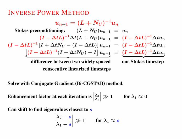
INVERSE POWER METHOD

un+1 = (L+NU)−1un

Stokes preconditioning: (L+NU)un+1 = un

(I −∆tL)−1∆t(L+NU)un+1 = (I −∆tL)−1∆tun

(I −∆tL)−1 [I + ∆tNU − (I −∆tL)]un+1 = (I −∆tL)−1∆tun[(I −∆tL)−1(I + ∆tNU)− I

]un+1

︸ ︷︷ ︸= (I −∆tL)−1∆tun

︸ ︷︷ ︸

difference between two widely spaced one Stokes timestep

consecutive linearized timesteps

Solve with Conjugate Gradient (Bi-CGSTAB) method.

Enhancement factor at each iteration is

∣∣∣λ2

λ1

∣∣∣≫ 1 for λ1 ≈ 0

Can shift to find eigenvalues closest to s∣∣∣∣

λ2 − s

λ1 − s

∣∣∣∣≫ 1 for λ1 ≈ s

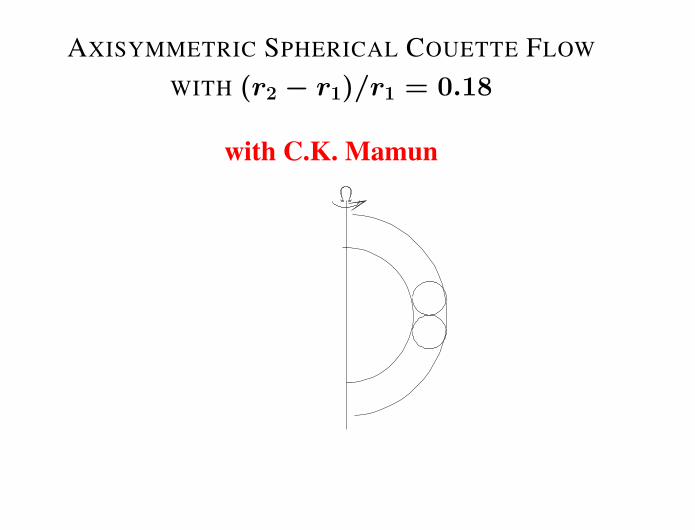
AXISYMMETRIC SPHERICAL COUETTE FLOW

WITH (r2 − r1)/r1 = 0.18

with C.K. Mamun

AXISYMMETRIC SPHERICAL COUETTE FLOW

AXISYMMETRIC SPHERICAL COUETTE FLOW

Basic flow at

Re = 650

Leading

eigenvector

Inverse Power Method on Spherical Couette Flow

∆t =100, 10, 1, 0.1, 0.01 s = −0.152,−0.15,−0.1, 0

CGcrit = 10−7(•, •), 10−9(△,△)s = −0.1, 0 M = 4096, 16384

OPTIMAL FORCING

with Mattias Brynjell-Rahkola, Philipp Schlatter, Dan Henningson, KTH

∂tu(x, t) = Au(x, t) + f(x)eiωt

u(x, t) = −(A− iωI)−1f(x)eiωt + eAtc(x)

=⇒ −(A− iωI)−1f(x)eiωt if all eigs ofA are negative

≡ −R(iω)f(x)eiωt

Seek profile f(x) and frequency ω which yields maximum

G(ω) = maxf(x)

||R(iω)f ||

||f ||

This is the maximum eigenvalue of

R(iω)R†(iω) =((A− iωI)(A† + iωI)

)−1

and f is the corresponding eigenvector.

Inverse power method with Laplacianpreconditioning again:

f (k+1) =((A− iωI)(A† + iωI)

)−1f (k) ⇐

(A− iωI)(A† + iωI)f (k+1) = f (k) ⇐

P(A− iωI)P†−1P†(A† + iωI)f (k+1) = Pf (k)

where P is the inverse of Laplacian or Stokes operator

Implement using actions withP,P† and solves withP(A−iωI),P†(A†+iωI):

g1 = Pf (k)

P(A− iωI)g2 = g1

g3 = P†g2

P†(A† + iωI)f (k+1) = g3

Tested on lid-driven cavity

Re=100

Re=8015

Forcing

Response

Performance of method for lid-driven cavity

Competing method uses forwards and backwards time integration

(e.g. Monokrousos, Akervik, Brandt, Henningson, JFM 2010)

SUMMARY

Time stepping Steady-state solving Linear stability analysis

∂tU = (N + L)U 0 = (N + L)U λu = (NU + L)u

Implicit/explicit Euler Newton Inverse power/Arnoldi

U(t+ ∆t) = BU(t) (NU + L)u (NU + L)un+1 = un= (I −∆tL)−1 = (N + L)U(I + ∆tN)U(t) U ← U − u

≡ P (I + ∆tN)U(t) AUu = AU AUun+1 = unPAUu = PAU PAUun+1 = Pun

3− 4 3− 4Newton steps Inverse Arnoldi steps

200 BiCGSTAB 200 BiCGSTAB

iters/step iters/step

BOSE-EINSTEIN CONDENSATION

Ultra-cold coherent state of matter

Predicted by Bose (1924) and Einstein (1925)

Realized experimentally by Cornell, Ketterle, Wieman (1995)

Nobel prize (2001)

Gross-Pitaevskii / Nonlinear Schrodinger Equation

∂tΨ = i [1

2∇2

︸ ︷︷ ︸L

+µ− V (r)− a|Ψ|2︸ ︷︷ ︸

N

]Ψ

V (x) =1

2|ω · x|2 =

1

2(ωrr

2 + ωzz2) (cylindrical trap)

Spatial discretisation up toM = 102 × 102 × 102 = 106

Eigenvalues, energies determine decay rates of condensate.

Hamiltonian Systems

f(A) = A

f(A) = eA∆t

f(A) = A−1

f(A) = A−2

STEADY STATE SOLVING:

0 = LΨ +N(Ψ)

Newton’s method + Stokes preconditioning + BICGSTAB

LINEAR STABILITY OF STEADY STATE Ψ:

∂tψ = i [(1

2∇2 + µ− V (r))ψ − aΨ2(2ψ + ψ∗)]

A

(ψR

ψI

)

≡

[0 −(L+DN I)

L+DNR 0

] (ψR

ψI

)

DNR ≡ µ− V (x)− 3aΨ2

DN I ≡ µ− V (x)− aΨ2

A2

(ψR

ψI

)

=

[−(L+DN I)(L+DNR) 0

0 −(L+DNR)(L+DN I)

] (ψR

ψI

)

Inverse square power with Stokes preconditioning and shift:

(A2 − s2I)ψn+1 = ψn

L−2(A2 − s2I)ψn+1 = L−2ψn

Solve with BICGSTAB

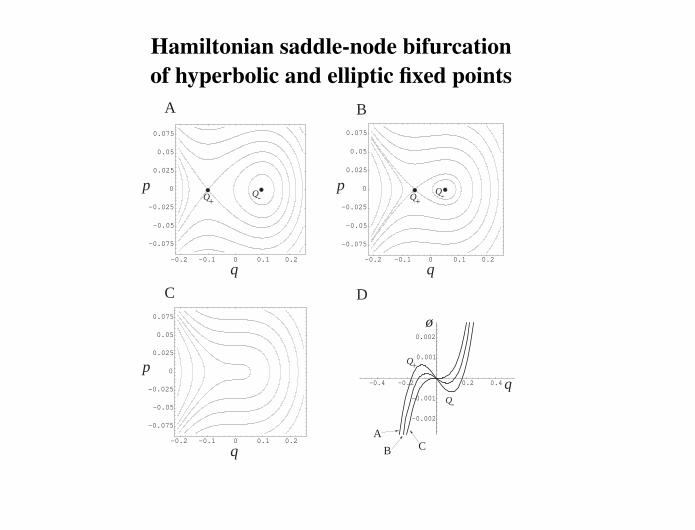
Hamiltonian saddle-node bifurcation

of hyperbolic and elliptic fixed points

-0.2 -0.1 0 0.1 0.2

-0.075

-0.05

-0.025

0

0.025

0.05

0.075

-0.2 -0.1 0 0.1 0.2

-0.075

-0.05

-0.025

0

0.025

0.05

0.075

-0.2 -0.1 0 0.1 0.2

-0.075

-0.05

-0.025

0

0.025

0.05

0.075

-0.4 -0.2 0.2 0.4

-0.002

-0.001

0.001

0.002

q

p

q

B

p

q

p

A

C D

q

ø

A

B C

Q

Q

Q QQ+ -

Q-+

+

-

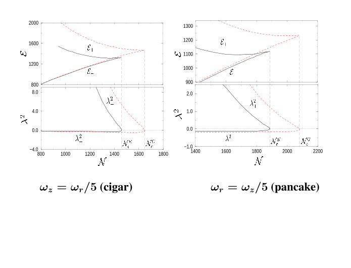
800

1200

1600

2000

800 1000 1200 1400 1600 1800−4.0

0.0

4.0

8.0

E

1

�

2

1

N

1

N

G

1

N

E

1

E

+

1

E

�

1

�

2

�

1

�

2

+

1

900

1000

1100

1200

1300

1400 1600 1800 2000 2200−1.0

0.0

1.0

2.0

N

1

E

�

1

E

1

�

2

1

N

E

1

N

G

1

E

+

1

�

2

+

1

�

2

�

1

ωz = ωr/5 (cigar) ωr = ωz/5 (pancake)

SUMMARY

Time stepping Steady-state solving Linear stability analysis

∂tU = (N + L)U 0 = (N + L)U λu = (NU + L)u

Implicit/explicit Euler Newton Inverse power/Arnoldi

U(t+ ∆t) = BU(t) (NU + L)u (NU + L)un+1 = un= (I −∆tL)−1 = (N + L)U(I + ∆tN)U(t) U ← U − u

≡ P (I + ∆tN)U(t) AUu = AU AUun+1 = unPAUu = PAU PAUun+1 = Pun

3− 4 3− 4Newton steps Inverse Arnoldi steps

200 BiCGSTAB 200 BiCGSTAB

iters/step iters/step