Bifador Modeling in Construct Validation of Multifactored ...glcanivez/Adobe pdf/Publications-Papers/Canivez...Validation of Multifactored Tests: Implications for Understanding

Bifador Modeling in Construct Validation of Multifactored Tests: Implications for Understanding Multidimensional Constructs and Test Interpretation

Gary L Canivez

Department of Psychology, Eastern Illinois University, Charleston, IL, USA

Factor analytic methods (exploratory [EFA] and confirmatory [CFA]) are integral parts of test development in both construction and later construct validation. Some examinations of test structure may originate at the item level, examining interrelationships or covariance among a set of items. Some examinations of test structure may originate at the subtest level, examining the interrelationships or covariance among a set of subtests. Yet another means of examination would be to examine interrelationships or covariance among items or subtests gathered from multiple different measures thought to measure the same or related latent constructs. Determining item or subtest retention and assignment to latent dimensions is a first step in test construction but understanding the latent dimensions captured by a psychological test and evaluating their psychometric characteristics is critical for application (interpretation) once the test is constructed. Interpretation of a test score from a unidimensional measure is rather straight forward as there will be only one score to report, but interpretation of scores produced by a multidimensional measure is more complicated and requires thorough examination and understanding of the reliability and validity of each of the provided scores as well as any comparisons between scores. The purpose and focus of this chapter is to present and illustrate use of the bifactor model, which is a model that is increasingly used for understanding the structure of multifactor tests and assisting in determining which scores can be appropriately interpreted. While bifactor modeling can also be applied to item level indicators, this was recently well illustrated with relationships to item response theory applications by Reise (2012) and thus, not included as part of this chapter. The bifactor model has important implications for both understanding the structure of a test as well as interpretation of various scores. To facilitate understanding and application of the bifactor model, comparisons are made to various

Canivez, G. L. (2016). Bifactor modeling in construct validation of multifactored tests: Implications for multidimensionality and test interpretation. In K. Schweizer & C. DiStefano (Eds.), Principles and methods of test construction: Standards and recent advancements (pp. 247–271). Gottingen, Germany: Hogrefe.

248 Principles and Methods of Test Construction

alternate models used to explain the interrelationships among a set of subtest indicators. Finally, a research example is used to illustrate exploratory and confirmatory bifactor modeling with one of the most popular and frequently used intelligence tests for children, the Wechsler Intelligence Scale for Children-Fourth Edition (WISC-IV; Wechsler, 2003). While bifactor modeling has primarily been applied to intelligence tests (see Canivez, 2011, 2014a; Canivez & Watkins, 2010a, 2010b; Chen, Hayes, Carver, Laurenceau, & Zhang, 2012; Gignac, 2005, 2006, 2008; Gignac & Watkins, 2013; Holzinger & Harman, 1938; Holzinger & Swineford, 1937; Watkins, 2006, 2010), it has been applied to personality tests (see Ackerman, Donnellan, & Robins, 2012; Chen et al., 2012) and psychopathology tests (see Brouwer, Meijer, & Zevalkink, 2013), but too few researchers and many fewer clinicians are familiar with its use even with intelligence tests.

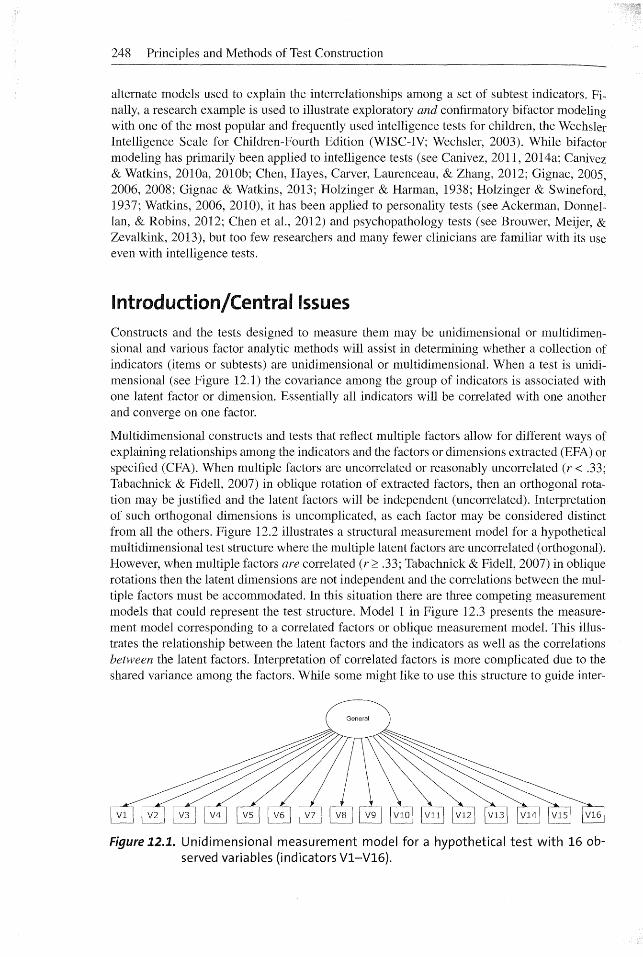
Introduction/Central Issues Constructs and the tests designed to measure them may be unidimensional or multidimensional and various factor analytic methods will assist in determining whether a collection of indicators (items or subtests) are unidimensional or multidimensional. When a test is unidimensional (see Figure 12.1) the covariance among the group of indicators is associated with one latent factor or dimension. Essentially all indicators will be correlated with one another and converge on one factor.

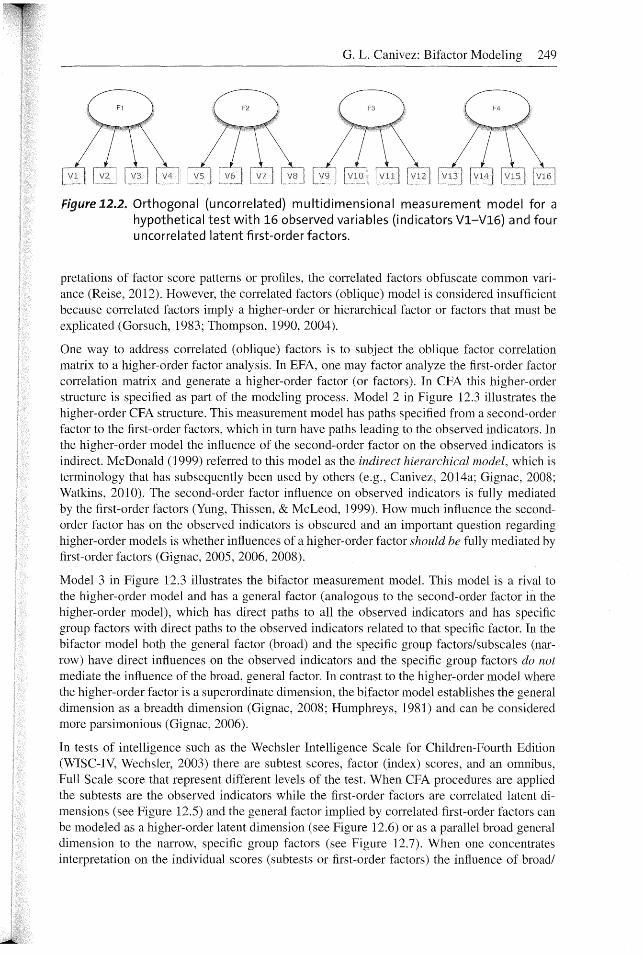
Multidimensional constructs and tests that reflect multiple factors allow for different ways of explaining relationships among the indicators and the factors or dimensions extracted (EFA) or specified (CFA). When multiple factors are uncorrelated or reasonably uncorrelated (r < .33; Tabachnick & Fidell, 2007) in oblique rotation of extracted factors, then an orthogonal rotation may be justified and the latent factors will be independent (uncorrelated). Interpretation of such orthogonal dimensions is uncomplicated, as each factor may be considered distinct from all the others. Figure 12.2 illustrates a structural measurement model for a hypothetical multidimensional test structure where the multiple latent factors are uncorrelated (orthogonal). However, when multiple factors are correlated (r :2: .33; Tabachnick & Fidell, 2007) in oblique rotations then the latent dimensions are not independent and the correlations between the multiple factors must be accommodated. In this situation there are three competing measurement models that could represent the test structure. Model 1 in Figure 12.3 presents the measurement model corresponding to a correlated factors or oblique measurement model. This illustrates the relationship between the latent factors and the indicators as well as the correlations between the latent factors. Interpretation of correlated factors is more complicated due to the shared variance among the factors. While some might like to use this structure to guide inter-

Figure 12.1. Unidimensional measurement model for a hypothetical test with 16 observed variables (indicators Vl-V16).

G. L. Canivez: Bifactor Modeling 249

Figure 12.2. Orthogonal (uncorrelated) multidimensional measurement model for a hypothetical test with 16 observed variables (indicators Vl-V16) and four uncorrelated latent first-order factors.

pretations of factor score patterns or profiles, the correlated factors obfuscate common variance (Reise, 2012). However, the correlated factors (oblique) model is considered insufficient because correlated factors imply a higher-order or hierarchical factor or factors that must be explicated (Gorsuch, 1983; Thompson, 1990, 2004).

One way to address correlated (oblique) factors is to subject the oblique factor correlation matrix to a higher-order factor analysis. In EFA, one may factor analyze the first-order factor correlation matrix and generate a higher-order factor (or factors). In CFA this higher-order structure is specified as part of the modeling process. Model 2 in Figure 12.3 illustrates the higher-order CFA structure. This measurement model has paths specified from a second-order factor to the first-order factors, which in turn have paths leading to the observed indicators. In the higher-order model the influence of the second-order factor on the observed indicators is indirect. McDonald (1999) referred to this model as the indirect hierarchical model, which is terminology that has subsequently been used by others (e.g., Canivez, 2014a; Gignac, 2008; Watkins, 2010). The second-order factor influence on observed indicators is fully mediated by the first-order factors (Yung, Thissen, & McLeod, 1999). How much influence the secondorder factor has on the observed indicators is obscured and an important question regarding higher-order models is whether influences of a higher-order factor should be fully mediated by first-order factors (Gignac, 2005, 2006, 2008).

Model 3 in Figure 12.3 illustrates the bifactor measurement model. This model is a rival to the higher-order model and has a general factor (analogous to the second-order factor in the higher-order model), which has direct paths to all the observed indicators and has specific group factors with direct paths to the observed indicators related to that specific factor. In the bifactor model both the general factor (broad) and the specific group factors/subscales (narrow) have direct influences on the observed indicators and the specific group factors do not mediate the influence of the broad, general factor. In contrast to the higher-order model where the higher-order factor is a superordinate dimension, the bifactor model establishes the general dimension as a breadth dimension (Gignac, 2008; Humphreys, 1981) and can be considered more parsimonious (Gignac, 2006).

In tests of intelligence such as the Wechsler Intelligence Scale for Children-Fourth Edition (WISC-IV, Wechsler, 2003) there are subtest scores, factor (index) scores, and an omnibus, Full Scale score that represent different levels of the test. When CFA procedures are applied the subtests are the observed indicators while the first-order factors are correlated latent dimensions (see Figure 12.5) and the general factor implied by correlated first-order factors can be modeled as a higher-order latent dimension (see Figure 12.6) or as a parallel broad general dimension to the narrow, specific group factors (see Figure 12.7). When one concentrates interpretation on the individual scores (subtests or first-order factors) the influence of broad/


Model 1

Model 2

Model 3

Figure 12.3. Three different multidimensional measurement models for a hypothetical test with 16 observed variables (indicators Vl-V16) and four latent first-order factors. Model 1 is the oblique (correlated) factor model, Model 2 is the higher-order (indirect hierarchical) factor model with one higher-order (H-0) and four lower-order (L-0) factors, and Model 3 is the bifactor (nested factor/ direct hierarchical) model with one general and four specific (S) factors.


general construct is conflated while concentration of interpretation on an omnibus, total score may miss important unique contributions provided by specific facets (Chen et al., 2012). For individuals it is not possible to disentangle the two sources of common variance (general and specific group factor). The bifactor model is less ambiguous than a higher-order model because it simultaneously discloses effects provided by a broad, general dimension while also disclosing effects of narrow, specific dimensions (Chen et al., 2012; Reise, 2012).

Conceptual Principles

The Bifactor Model

The bifactor model was first proposed and illustrated by Holzinger and Swineford (1937) and Holzinger and Harman (1938), although their method is no longer used (Jennrich & Bentler, 2011). There are both exploratory and confirmatory approaches to bifactor modeling. Alternate names for the bifactor model that appear in the literature include the nested factors model (Gustafsson & Balke, 1993) and the direct hierarchical model (e.g., Canivez, 2014a; Gignac, 2008, McDonald, 1999; Watkins, 2010). Gignac's original use of the term direct hierarchical was influenced by McDonald and relates to the direct influence of the general factor on subtest indicators in a bifactor model as opposed to the indirect hierarchical influence of the general factor on subtests mediated by first-order factors (Gignac, 2008; McDonald, 1999).

The bifactor model offers a number of key advantages including: 1. The general factor is easy to interpret with direct influences on indicators as this implies

inferences directly from the subtest indicators rather than inferences from inferences (factors) (or interpretations based on other interpretations) present in the higher-order model, which Gorsuch (1983) noted was ambiguous;

2. Both general and specific influences on indicators (subtests) can be examined simultaneously, which allows for judgments of general and specific group scale importance (Gorsuch, 1983; Reise, 2012; Reise, More, & Haviland, 2010);

3. The psychometric properties necessary for determining scoring and interpretation of the general dimension and subscales may be examined (i.e., model based reliability using Omega-hierarchical and Omega-subscale [Reise, 2012; Zinbarg, Yovel, Revelle, & McDonald, 2006]); and

4. Unique contributions of the general and specific group factors in predicting external criteria or variables may be assessed (Chen et al., 2012; Chen, West, & Sousa, 2006; Gignac, 2006, 2008; Reise et al., 2010).

Exploratory Bifactor Model

The exploratory bifactor model has historically and most frequently been estimated by the Schmid and Leiman (1957) orthogonalization procedure (Jennrich & Bentler, 2011; Reise, 2012). The Schmid-Leiman (SL) procedure transforms "an oblique factor analysis solution containing a hierarchy of higher-order factors into an orthogonal solution which not only preserves the desired interpretation characteristics of the oblique solution, but also discloses the hierarchical structuring of the variables" (Schmid & Leiman, 1957, p. 53). It is a reparameterization of a higher-order model (Reise, 2012). Thus, subtest or indicator common variance is apportioned first to the higher-order factor and the residual common variance is then apportioned to the lower-order factors. This solution, "not only preserves the desired interpretation


characteristics of the oblique solution, but also discloses the hierarchical structuring of the variables" (Schmid & Leiman, 1957, p. 53). It is this feature that led Carroll (1995) to insist on SL orthogonalization of higher-order models:

I argue, as many have done, that from the standpoint of analysis and ready interpretation, results should be shown on the basis of orthogonal factors, rather than oblique, correlated factors. I insist, however, that the orthogonal factors should be those produced by the Schmid-Leiman ( 1957) orthogonalization procedure, and thus include second-stratum and possibly third-stratum factors. (p. 437)

Procedurally the first step in the traditional method of exploratory bifactor modeling is conducting an exploratory factor analysis (principal factors) of the subtests or indicators using an oblique rotation. Following the oblique rotation a second-order exploratory factor analysis of the first-order factor correlation matrix would be conducted. Next the Schmid-Leiman transformation would be applied to apportion subtest or indicator variance to the higher-order dimension and the lower-order specific group factors. The MacOrtho program produced by Watkins (2004) is available for Mac and Windows OS and is perhaps the easiest to use and is based on the instructions provided by Thompson (2004). MacOrtho is available as freeware from http://www.edpsychassociates.com. Thompson (1990) also described this procedure and SPSS syntax is also provided in Thompson (2004 ). Wolff and Preising (2005) also provided SPSS and SAS syntax code for the SL procedure. From the MacOrtho results, which provide orthogonal standardized coefficients of subtest or indicator loadings with the higher-order and lower-order factors, one may square the loadings to yield variance estimates (see Table 12.3). Results then disclose the portions of subtest or indicator variance associated with the general higher-order factor and the variance associated with the specific first-order factor. In this exploratory bifactor solution subtest variance attributable to alternate first-order factors will also be disclosed (i.e., cross-loadings).

While the SL procedure is the most commonly used method for estimating an exploratory bifactor model it is not without some potential limitations. As pointed out by Yung et al. (1999) and others (Chen et al., 2006; Reise, 2012) the SL transformation of a higher-order model includes a proportionality constraint of general and specific variance ratios. Reise (2012) also noted that nonzero cross-loadings are problematic and the larger the cross-loadings the greater the distortion of overestimating general factor loadings and underestimating specific group factor loadings. Such cross-loadings might suggest problems with the scale content, however. As stated by Brunner, Nagy, and Wilhelm (2012):

The proportionality constraint limits the value of the higher order factor model in providing insights into the relationship between general and specific abilities, on the one hand, and other psychological constructs, sociodemographic characteristics, or life outcomes, on the other. (p. 811)

However, how prevalent this is with real data is as yet unknown (Jennrich & Bentler, 2011) and it is possible that this issue may be more theoretical than real. Bifactor models, however, do not suffer from such proportionality constraints.

Recently, several exploratory bifactor modeling alternatives have been developed. Jennrich and Bentler (2011) reported on the development of an exploratory bifactor analysis using an orthogonal bifactor rotation criterion and related it to the SL procedure while Jennrich and Bentler (2012) reported on the development of an exploratory bifactor analysis using an oblique bifactor rotation criterion. These will likely be the topic of comparative research in the coming years and may offer useful alternatives to the SL procedure. Finally, Reise, Moore, and Maydeu-Oliveres (2011) developed and evaluated a target bifactor rotation method. These


three exploratory bifactor methods avoid the proportionality constraints of the SL procedure applied to higher-order models. Dombrowski (2014b) compared EFA results from the SL procedure and the exploratory bifactor analysis (Jennrich & Bentler, 2012) and found similar results suggesting Reise et al. (2010) may be correct that proportionality constraint may be inconsequential with real data.

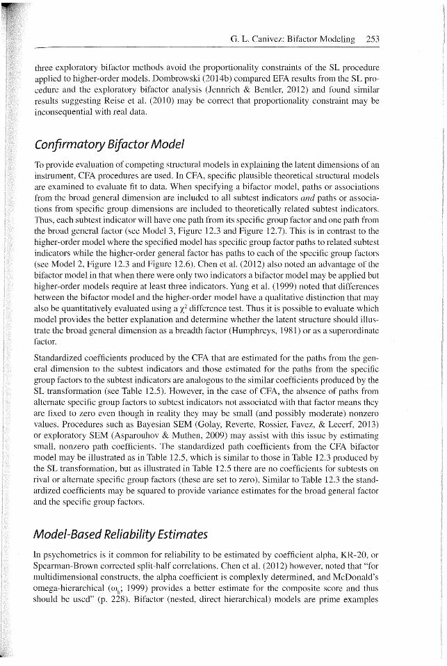
Confirmatory Bifactor Model

To provide evaluation of competing structural models in explaining the latent dimensions of an instrument, CFA procedures are used. In CFA, specific plausible theoretical structural models are examined to evaluate fit to data. When specifying a bifactor model, paths or associations from the broad general dimension are included to all subtest indicators and paths or associations from specific group dimensions are included to theoretically related subtest indicators. Thus, each subtest indicator will have one path from its specific group factor and one path from the broad general factor (see Model 3, Figure 12.3 and Figure 12.7). This is in contrast to the higher-order model where the specified model has specific group factor paths to related subtest indicators while the higher-order general factor has paths to each of the specific group factors (see Model 2, Figure 12.3 and Figure 12.6). Chen et al. (2012) also noted an advantage of the bifactor model in that when there were only two indicators a bifactor model may be applied but higher-order models require at least three indicators. Yung et al. (1999) noted that differences between the bifactor model and the higher-order model have a qualitative distinction that may also be quantitatively evaluated using a x2 difference test. Thus it is possible to evaluate which model provides the better explanation and determine whether the latent structure should illustrate the broad general dimension as a breadth factor (Humphreys, 1981) or as a superordinate factor.

Standardized coefficients produced by the CFA that are estimated for the paths from the general dimension to the subtest indicators and those estimated for the paths from the specific group factors to the subtest indicators are analogous to the similar coefficients produced by the SL transformation (see Table 12.5). However, in the case of CFA, the absence of paths from alternate specific group factors to subtest indicators not associated with that factor means they are fixed to zero even though in reality they may be small (and possibly moderate) nonzero values. Procedures such as Bayesian SEM (Golay, Reverte, Rossier, Favez, & Lecerf, 2013) or exploratory SEM (Asparouhov & Muthen, 2009) may assist with this issue by estimating small, nonzero path coefficients. The standardized path coefficients from the CFA bifactor model may be illustrated as in Table 12.5, which is similar to those in Table 12.3 produced by the SL transformation, but as illustrated in Table 12.5 there are no coefficients for subtests on rival or alternate specific group factors (these are set to zero). Similar to Table 12.3 the standardized coefficients may be squared to provide variance estimates for the broad general factor and the specific group factors.

Model-Based Reliability Estimates

In psychometrics is it common for reliability to be estimated by coefficient alpha, KR-20, or Spearman-Brown corrected split-half correlations. Chen et al. (2012) however, noted that "for multidimensional constructs, the alpha coefficient is complexly determined, and McDonald's omega-hierarchical (w

11; 1999) provides a better estimate for the composite score and thus

should be used" (p. 228). Bifactor (nested, direct hierarchical) models are prime examples


where the variance of each observed measure is complexly determined and "omega hierarchical is an appropriate model-based reliability index when item response data are consistent with a bifactor structure" (Reise, 2012, p. 689). The same may be applied when subtests are the indicators. A prerequisite to using omega is a well-fitting, completely orthogonal bifactor model. While calculating decomposed variance estimates for SL transformed higher-order structures or bifactor models is common, calculation of omega is not, but is increasing (see Canivez, 2014a; Canivez & Watkins, 2010a, 2010b; Dombrowski, 2014a).

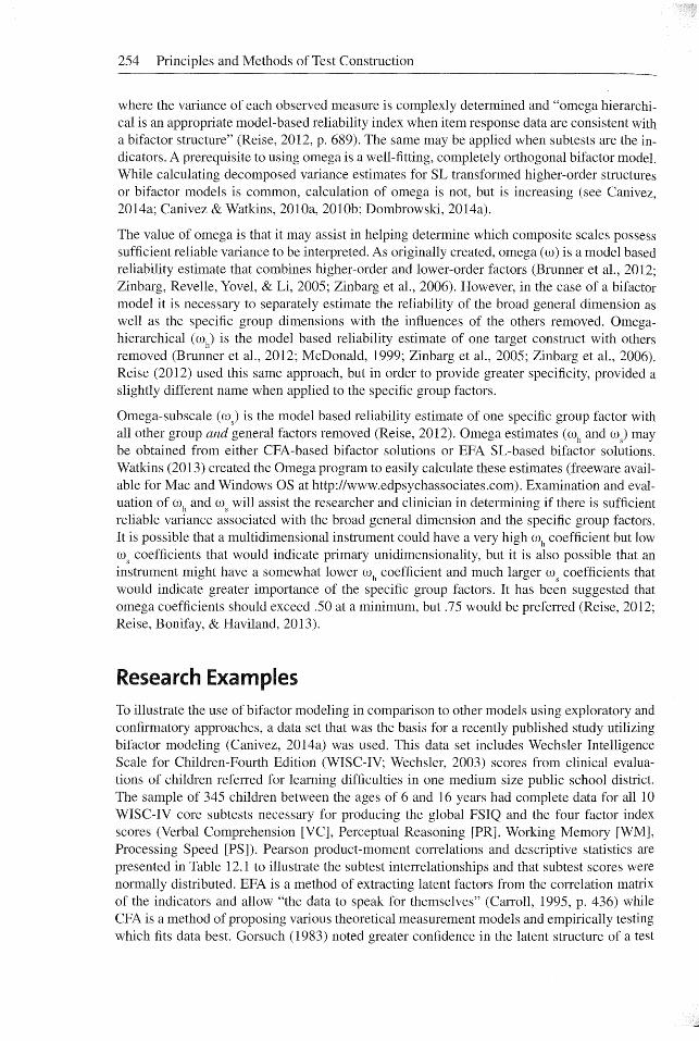
The value of omega is that it may assist in helping determine which composite scales possess sufficient reliable variance to be interpreted. As originally created, omega ( w) is a model based reliability estimate that combines higher-order and lower-order factors (Brunner et al., 2012; Zinbarg, Revelle, Yovel, & Li, 2005; Zinbarg et al., 2006). However, in the case of a bifactor model it is necessary to separately estimate the reliability of the broad general dimension as well as the specific group dimensions with the influences of the others removed. Omegahierarchical ( wh) is the model based reliability estimate of one target construct with others removed (Brunner et al., 2012; McDonald, 1999; Zinbarg et al., 2005; Zinbarg et al., 2006). Reise (2012) used this same approach, but in order to provide greater specificity, provided a slightly different name when applied to the specific group factors.

Omega-subscale (w) is the model based reliability estimate of one specific group factor with all other group and general factors removed (Reise, 2012). Omega estimates (wh and w) may be obtained from either CPA-based bifactor solutions or EPA SL-based bifactor solutions. Watkins (2013) created the Omega program to easily calculate these estimates (freeware available for Mac and Windows OS at http://www.edpsychassociates.com). Examination and evaluation of wh and W

8 will assist the researcher and clinician in determining if there is sufficient

reliable variance associated with the broad general dimension and the specific group factors. It is possible that a multidimensional instrument could have a very high wh coefficient but low W

8 coefficients that would indicate primary unidimensionality, but it is also possible that an

instrument might have a somewhat lower wh coefficient and much larger W8

coefficients that would indicate greater importance of the specific group factors. It has been suggested that omega coefficients should exceed .50 at a minimum, but .75 would be preferred (Reise, 2012; Reise, Bonifay, & Haviland, 2013).

Research Examples To illustrate the use of bifactor modeling in comparison to other models using exploratory and confirmatory approaches, a data set that was the basis for a recently published study utilizing bifactor modeling (Canivez, 2014a) was used. This data set includes Wechsler Intelligence Scale for Children-Fourth Edition (WISC-IV; Wechsler, 2003) scores from clinical evaluations of children referred for learning difficulties in one medium size public school district. The sample of 345 children between the ages of 6 and 16 years had complete data for all 10 WISC-IV core subtests necessary for producing the global PSIQ and the four factor index scores (Verbal Comprehension [VC], Perceptual Reasoning [PR], Working Memory [WM], Processing Speed [PS]). Pearson product-moment correlations and descriptive statistics are presented in Table 12.1 to illustrate the subtest interrelationships and that subtest scores were normally distributed. EPA is a method of extracting latent factors from the correlation matrix of the indicators and allow "the data to speak for themselves" (Carroll, 1995, p. 436) while CPA is a method of proposing various theoretical measurement models and empirically testing which fits data best. Gorsuch (1983) noted greater confidence in the latent structure of a test


when both EFA and CFA were in agreement. Carroll (1995) and Reise (2012) noted that EFA procedures are particularly useful in suggesting possible models to be tested in CFA. What fol-lows are EFA and CFA illustrating application of bifactor solutions in understanding the latent structure of the WISC-IV with the referred sample of 345 children.

Table 12.1. Pearson correlations and descriptive statistics for Wechsler Intelligence Scale for Children-Fourth Edition (WISC-IV) core subtests with a referred sample (N = 345)

Subtest BD SI DS PCn CD VO LN MR co SS

Block Design (BD)

Similarities (SI) .539

Digit Span (DS) .397 .386

Picture .501 .489 .368 Concepts (PCn)

Coding (CD) .257 .242 .217 .313

Vocabulary .503 .732 .417 .467 .267 (VO)

Letter-Number .462 .439 .459 .470 .291 .560 Sequencing (LN)

Matrix .701 .517 .393 .507 .295 .555 .511 Reasoning (MR)

Comprehension .426 .643 .404 .484 .342 .723 .499 .462 (CO)

Symbol Search .518 .423 .383 .399 .511 .472 .428 .515 .428 (SS)

M 7.660 7.840 7.590 9.080 7.550 7.380 7.310 8.320 8.090 7.850

50 3.251 2.928 2.909 3.203 2.724 2.969 3.221 3.090 2.812 3.271

5k 0.270 0.513 0.310 -0.279 0.123 0.453 -0.211 0.188 -0.180 -0.269

K -0.389 0.255 0.295 -0.256 -0.081 0.517 -0.520 0.037 0.079 -0.551

Note. 5k =skewness; K =kurtosis. Mardia's (1970) multivariate kurtosis estimate was 1.17.

Example 1: Exploratory Bifactor Analysis With the SL Method

Principal axis (principal factors) EFA (SPSS v. 21) produced a Kaiser-Meyer-Olkin measure of sampling adequacy coefficient of .894 (exceeding the .60 criterion; Tabachnick & Fidell, 2007) and Bartlett's Test of Sphericity was 1,663.05, p < .0001, indicating that the correlation matrix was not random. Communality estimates ranged from .337 to .994 (Mdn = .666). Given the communality estimates, number of variables, and factors, the sample size was judged adequate for factor analytic procedures (Fabrigar, Wegener, MacCallum, & Strahan, 1999; Floyd & Widaman, 1995; MacCallum, Widaman, Zhang, & Hong, 1999). Multiple criteria as recommended by Gorsuch (1983) were examined and included eigenvalues> l (Guttman, 1954), visual scree test (Cattell, 1966), standard error of scree (SEscree; Zoski & Jurs, 1996) as recommended by Nasser, Benson, and Wisenbaker (2002) and programmed by Watkins (2007), Horn's parallel analysis (HPA; Horn, 1965) as programmed by Watkins (2000) with 100 replications (see Figure 12.4), and minimum average partials (MAP; Velicer, 1976) using the SPSS code supplied by O'Connor (2000). All criteria indicated only one factor should be


4.00

(!) :::;

(ii > 3.00 c (!) OJ w

2.00

10

Factor

Figure 12.4. Scree plots for Horn's parallel analysis for the 10 WISC-IV core subtests with a referred sample (N = 345).

extracted (illustrating the dominance of the general intelligence dimension) but theory suggested four latent first-order factors (VC, PR, WM, PS).

To explore and illustrate the WISC-IV multidimensional structure, four factors were extracted and obliquely rotated with promax (k = 4; Gorsuch, 2003). Results are presented in Table 12.2 and show that when four factors were extracted to be consistent with the underlying theory, 9 of the 10 WISC-IV core subtests demonstrated salient factor pattern coefficients (:2.:: .30; Child, 2006) on the theoretically consistent factor but one salient cross-loading on an alternate factor was observed (Symbol Search). The Picture Concepts subtest did not have a salient coefficient on any of the four factors although its highest factor pattern coefficient was on the theoretically consistent factor (PR). Symbol Search, however, had its highest pattern coefficient on a theoretically inconsistent factor (PR) that was slightly higher than the pattern coefficient on its theoretically consistent factor (PS). These anomalies are likely due to sampling error as such findings are rarely obtained. Of greater importance, however, are the correlations between the four extracted factors (see Table 12.2). The moderate to high factor correlations (.398 to .729) imply a higher-order or hierarchical factor that requires explication (Gorsuch, 1983; Thompson, 1990, 2004) and thus ending analyses at this point is premature for full understanding of the WISC-IV structure.

The four first-order factors were then orthogonalized using the Schmid and Leiman (SL, 1957) procedure as programmed in the MacOrtho computer program (Watkins, 2004 ), which uses the procedure described in Thompson (1990). Carroll (1995) insisted that correlated factors be orthogonalized by the SL procedure and, as stated by Schmid & Leiman (1957), this transforms:

An oblique factor analysis solution containing a hierarchy of higher-order factors into an orthogonal solution which not only preserves the desired interpretation characteristics of the oblique solution, but also discloses the hierarchical structuring of the variables. (p. 53)

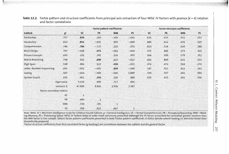
Table 12.2. Factor pattern and structure coefficients from principal axis extraction of four WISC-IV factors with promax (k = 4) rotation and factor correlations

Subtest g• vc Similarities .757 .839

Vocabulary .812 .852

Comprehension .746 .784

Block Design .747 -.028

Picture Concepts .643 .192

Matrix Reasoning .748 .042

Digit Span .548 .084

Letter-Number Sequencing .695 -.002

Coding .507 -.014

Symbol Search .655 .061

Eigenvalue 5.134

variance% 47.889

Factor correlation matrix

vc 1

PR .689

WM .729

PS .398

Factor pattern coefficients

PR

.183

-.021

-.133

.972

.281

.690

.123

-.005

-.040

.356

.990

8.826

1

.701

.422

WM

-.169

.093

.120

-.062

.216

.123

.428

.839

-.046

.120

.727

2.936

1

.467

Factor structure coefficients

PS vc PR WM PS

-.042 .826 .625 .552 .291

-.049 .886 .611 .676 .325

.076 .810 .524 .634 .388

-.056 .575 .886 .573 .315

.055 .566 .589 .579 .352

-.013 .602 .800 .631 .353

-.015 .474 .474 .568 .270

-.049 .587 .562 .812 .341

1.037 .339 .357 .401 .994

.315 .520 .615 .561 .546

.806

5.387

1

Note. WISC-IV= Wechsler Intelligence Scale for Children-Fourth Edition; g =General Intelligence; VC =Verbal Comprehension; PR= Perceptual Reasoning; WM= Working Memory; PS= Processing Speed. WISC-IV factors listed in order most commonly presented although the PS factor accounted for somewhat greater variance than the WM factor in this sample. Salient factor pattern coefficients presented in bold. Factor pattern coefficients in italics denote salient loading on alternate factor than theoretically proposed. •Factor structure coefficients from first unrotated factor (g-loadings} are correlations between the subtest and the general factor.


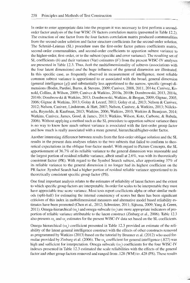
In order to enter appropriate data into the program it was necessary to first perform a secondorder factor analysis of the four WISC-IV factors correlation matrix (presented in Table 12.2). The extraction of one factor from the four factors correlation matrix produced communalities from the second-order solution and factor structure coefficients for the second-order solution. The Schmid-Leiman (SL) procedure uses the first-order factor pattern coefficients matrix, second-order communalities, and second-order coefficients to apportion subtest variance to the higher-order, first-order, or to the subtest (specific and error variance). The resulting set of SL coefficients (b) and their variance (Var) estimates (b2

) from the present WISC-IV analyses are presented in Table 12.3. Thus, both the multidimensionality of subtests (associations with the four latent dimensions) and the huge influence of the general dimension are illustrated. In this specific case, as frequently observed in measurement of intelligence, most reliable common subtest variance is apportioned to or associated with the broad, general dimension (general intelligence [g]) and substantially less apportioned to the narrow, specific (group) dimensions (Bodin, Pardini, Burns, & Stevens, 2009; Canivez, 2008, 2011, 2014a; Canivez, Konold, Collins, & Wilson, 2009; Canivez & Watkins, 2010a, 2010b; Dombrowski, 2013, 2014a, 2014b; Dombrowski & Watkins, 2013; Dombrowski, Watkins, & Brogan, 2009; Gignac, 2005, 2006; Gignac & Watkins, 2013; Golay & Lecerf, 2011; Golay et al., 2013; Nelson & Canivez, 2012; Nelson, Canivez, Lindstrom, & Hatt, 2007; Nelson, Canivez, & Watkins, 2013; Niilekssela, Reynolds, & Kaufman, 2013; Watkins, 2006; Watkins, 2010, Watkins & Beaujean, 2014; Watkins, Canivez, James, Good, & James, 2013; Watkins, Wilson, Kotz, Carbone, & Babula, 2006). Without applying a method such as the SL procedure to apportion subtest variance there is no way to know how much subtest variance is associated with the first-order group factor and how much is really associated with a more general, hierarchical/higher-order factor.

Another interesting difference between results from the first-order oblique solution and the SL results in the present data analyses relates to the two subtests that failed to conform to theoretical expectations in the oblique four-factor model. With regard to Picture Concepts, the SL apportionment of 36.7% of its reliable variance to the general dimension was reasonable and the largest portion of residual reliable variance, albeit small at 2.6%, was with its theoretically consistent factor (PR). With regard to the Symbol Search subtest, after apportioning 37% of its reliable variance to the general dimension it no longer had its highest coefficient on the PR factor. Symbol Search had a higher portion of residual reliable variance apportioned to its theoretically consistent specific group factor (PS).

One final important analysis relates to the estimates of reliability of latent factors and the extent to which specific group factors are interpretable. In order for scales to be interpretable they must have appreciable true score variance. Most tests report coefficients alpha or other similar methods (split-half) for estimating the internal consistency of scores but there has been significant criticism of this index in multidimensional measures and alternative model based reliability estimates have been promoted (Chen et al., 2012; Schweizer, 2011; Sijtsma, 2009; Yang & Green, 2011 ). Omega-hierarchical ( wh) and omega-subscale ( w) are more appropriate indicators of proportion of reliable variance attributable to the latent construct (Zinbarg et al., 2006). Table 12.3 also presents wh and w s estimates for the present WISC-IV data set based on the SL coefficients.

Omega hierarchical (wh) coefficient presented in Table 12.3 provided an estimate of the reli-· ability of the latent general intelligence construct with the effects of other constructs removed as programmed by Watkins (2013) based on the tutorial by Brunner et al. (2012) who used formulae provided by Zinbarg et al. (2006). The wh coefficient for general intelligence (.827) was high and sufficient for interpretation. Omega subscale (ws) coefficients for the four WISC-IV indexes presented in Table 12.3 estimated the scale reliabilities with the effects of the general factor and other group factors removed and ranged from .128 (WM) to .428 (PS). These results

Table 12.3. Sources of variance in the Wechsler Intelligence Scale for Children-Fourth Edition for the referred sample (N = 345) according to an orthogonalized (Schmid & Lei man, 1957) higher-order factor model

General vc PR WM PS

Subtest b Var b Var b Var b Var b Var h2 u2

Similarities .676 .457 .469 .220 .106 .011 -.082 .007 -.036 .001 .696 .304

Vocabulary .746 .557 .477 .228 -.012 .000 .045 .002 -.042 .002 .788 .212

Comprehension .685 .469 .439 .193 -.077 .006 .058 .003 .065 .004 .675 .325

Block Design .688 .473 -.016 .000 .561 .315 -.030 .001 -.048 .002 .792 .208

Picture Concepts .606 .367 .107 .011 .162 .026 .104 .011 .047 .002 .418 .582

Matrix Reasoning .700 .490 .023 .001 .398 .158 .059 .003 -.011 .000 .653 .347

Digit Span .537 .288 .047 .002 .071 .005 .207 .043 -.013 .000 .339 .661

Letter-Number Sequencing .704 .496 -.001 .000 -.003 .000 .405 .164 -.042 .002 .661 .339 p Coding .426 .181 -.008 .000 -.023 .001 -.022 .000 .859 .738 .920 .080 r Symbol Search .608 .370 .034 .001 .205 .042 .058 .003 .271 .073 .490 .510 n

~

% Total Variance 41.5 6.6 5.6 2.4 8.3 64.3 35.7 :;:I ~2" (D

% Common Variance 64.5 10.2 8.8 3.7 12.8 100 ~

Wh=.827 W5= .265 w = .196 W

5= .128 W

5=.428

ttl s ~

Note. b =Standardized loading of subtest on factor; Var= variance (b2) explained in the subtest; h2 =communality; u2 =uniqueness; VC =Verbal Comprehension; PR= () ...... 0

Perceptual Reasoning; WM= Working Memory; PS= Processing Speed; wh =Omega Hierarchical; W5 =Omega Subscale. Largest first-order factor coefficients presented I-!

in bold. ~ 0 0... g_ s·

CfQ

N U1 \0


indicated that in the present sample the four specific WISC-IV group factors possessed too little reliable variance for clinicians to confidently interpret (Reise, 2012; Reise et al., 2013).

Example 2: Confirmatory Bifactor Analysis The present data set was used in the CFA study recently published (Canivez, 2014a). In the CFA approach various measurement models that are theoretically possible explanations for the covariance among indicators are specified and compared. With respect to the WISC-IV, theoretical and historical structures that have evolved have included a unidimensional (general intelligence) model, a two-factor model (verbal and performance), three-factor model (verbal comprehension, perceptual organization, freedom from distractibility), and a four-factor model (verbal comprehension, perceptual reasoning, working memory, processing speed). The two-, three-, and four-factor models all have correlated factors so examination of higher-order and bifactor models that account for the correlated first-order dimensions are also needed.

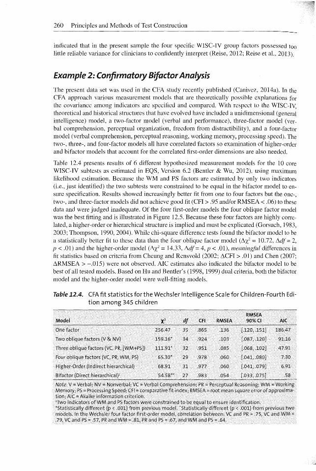
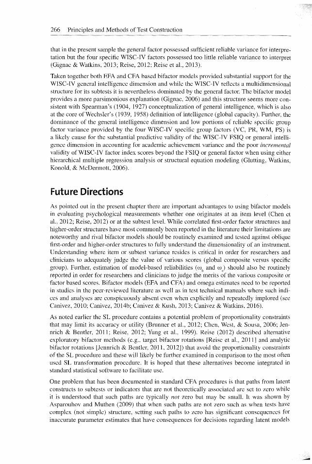
Table 12.4 presents results of 6 different hypothesized measurement models for the 10 core WISC-IV subtests as estimated in EQS, Version 6.2 (Bentler & Wu, 2012), using maximum likelihood estimation. Because the WM and PS factors are estimated by only two indicators (i.e., just identified) the two subtests were constrained to be equal in the bifactor model to ensure specification. Results showed increasingly better fit from one to four factors but the one-, two-, and three-factor models did not achieve good fit (CFI > .95 and/or RMSEA < .06) to these data and were judged inadequate. Of the four first-order models the four oblique factor model was the best fitting and is illustrated in Figure 12.5. Because these four factors are highly correlated, a higher-order or hierarchical structure is implied and must be explicated (Gorsuch, 1983, 2003; Thompson, 1990, 2004). While chi-square difference tests found the bifactor model to be a statistically better fit to these data than the four oblique factor model (~X2 = 10. 72, ~df = 2, p < .01) and the higher-order model (~X2 = 14.33, ~df = 4, p < .01), meaningful differences in fit statistics based on criteria from Cheung and Rensvold (2002; ~CFI > .01) and Chen (2007; ~RMSEA > -.015) were not observed. AIC estimates also indicated the bifactor model to be best of all tested models. Based on Hu and Bentler's (1998, 1999) dual criteria, both the bifactor model and the higher-order model were well-fitting models.

Table 12.4. CFA fit statistics for the Wechsler Intelligence Scale for Children-Fourth Edition among 345 children

RMS EA Model CFI RMS EA 90%CI AIC

One factor 256.47 35 .865 .136 [.120, .151] 186.47

Two oblique factors (V & NV) 159.16* 34 .924 .103 [.087, .120] 91.16

Three oblique factors (VC, PR, [WM+PS]) 111.91 * 32 .951 .085 [.068, .102] 47.91

Four oblique factors (VC, PR, WM, PS) 65.30* 29 .978 .060 [.041, .080] 7.30

Higher-Order (Indirect hierarchical) 68.91 31 .977 .060 [.041, .079] 6.91

Bifactor (Direct hierarchical)a 54.58** 27 .983 .054 [.033, .075] .58

Note. V =Verbal; NV= Nonverbal; VC =Verbal Comprehension; PR= Perceptual Reasoning; WM= Working Memory; PS= Processing Speed; CFI =comparative fit index; RMSEA =root mean square error of approximation; AIC = Akaike information criterion. aTwo indicators of WM and PS factors were constrained to be equal to ensure identification. *Statistically different (p < .001) from previous model. "Statistically different (p < .001) from previous two models. In the Wechsler four factor first-order model, correlation between: VC and PR= .75, VC and WM= .79, VC and PS= .57, PR and WM= .81, PR and PS= .67, and WM and PS= .64.


Figure 12.5. Oblique (correlated) four-factor measurement model, with standardized coefficients, for the Wechsler Intelligence Scale for Children-Fourth Edition {Wechsler, 2003) for 345 referred children; SI = Similarities, VO = Vocabulary, CO= Comprehension, BD = Block Design, PCn = Picture Concepts, MR =Matrix Reasoning, DS = Digit Span, LN = Letter-Number Sequencing, CD =Coding, and SS= Symbol Search, VC =Verbal Comprehension factor, PR= Perceptual Reasoning factor, WM =Working Memory factor, PS = Processing Speed factor.


.81

co .83

.81

.61

.75

.72

CD .56

.92

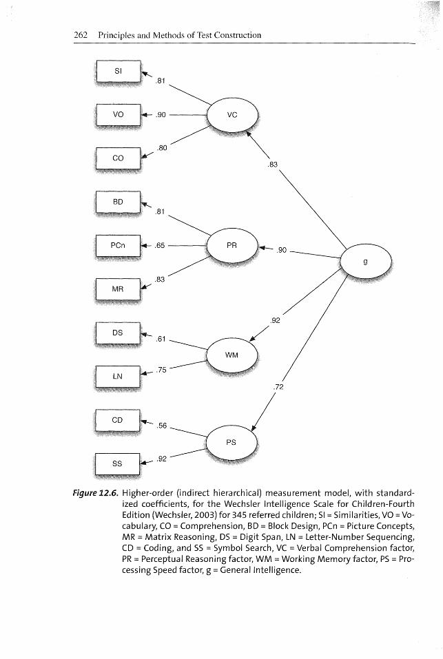
Figure 12.6. Higher-order (indirect hierarchical) measurement model, with standardized coefficients, for the Wechsler Intelligence Scale for Children-Fourth Edition (Wechsler, 2003) for 345 referred children; SI= Similarities, VO= Vocabulary, CO= Comprehension, BD = Block Design, PCn = Picture Concepts, MR= Matrix Reasoning, DS = Digit Span, LN =Letter-Number Sequencing, CD =Coding, and SS =Symbol Search, VC =Verbal Comprehension factor, PR= Perceptual Reasoning factor, WM =Working Memory factor, PS= Processing Speed factor, g =General Intelligence.


.42

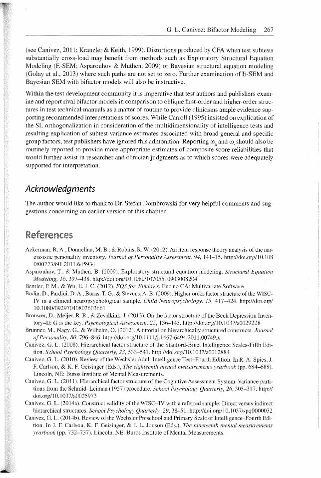
Figure 12.7. Bifactor (nested factors/direct hierarchical) measurement model, with standardized coefficients, for the Wechsler Intelligence Scale for ChildrenFourth Edition (Wechsler, 2003) for 345 referred children; SI= Similarities, VO =Vocabulary, CO = Comprehension, BD = Block Design, PCn = Picture Concepts, MR = Matrix Reasoning, DS = Digit Span, LN = Letter-Number Sequencing, CD = Coding, and SS = Symbol Search, VC =Verbal Comprehension factor, PR = Perceptual Reasoning factor, WM =Working Memory factor, PS= Processing Speed factor, g =General Intelligence.

Table 12.5. Sources of variance in the Wechsler Intelligence Scale for Children-Fourth Edition for the referred sample (N = 345) according to the bifactor (nested factor/direct hierarchical) model

Subtest

Similarities

Vocabulary

Comprehension

Block Design

Picture Concepts

Matrix Reasoning

Digit Span

Letter-Number Sequencing

Coding

Symbol Search

% Total variance

% Common variance

General

b

.691

.742

.675

.708

.663

.741

.561

.692

.405

.652

Var

.477

.551

.456

.501

.440

.549

.315

.479

.164

.425

43.6

71.6

Wh= .843

b

.417

.525

.423

vc

6.3

10.3

Var

.174

.276

.179

w,= .259

b

.605

.052

.290

PR

4.5

7.4

Var

.366

.003

.084

W5= .140

b

.281

.254

WM

1.4

2.4

Var

.079

.065

W5= .098

b

.545

.454

PS

5.0

8.3

Var

.297

.206

h2

.651

.826

.635

.867

.442

.633

.394

.543

.461

.631

60.8

100

u2

.349

.174

.365

.133

.558

.367

.606

.457

.539

.369

39.2

Note. b =Standardized loading of subtest on factor; Var= variance (b2} explained in the subtest; h2 =communality; u2 =uniqueness; VC =Verbal Comprehension; PR= Perceptual Reasoning; WM= Working Memory; PS= Processing Speed; wh =Omega Hierarchical; W

5 =Omega Subscale.


To understand differences between the higher-order model (Figure 12.6) and the bifactor model (Figure 12.7) it is useful to compare the two rival measurement models. The standardized measurement model for the higher-order model in Figure 12.6 illustrates high standardized path coefficients from the first-order factors to their subtest indicators as well as the high standardized path coefficients from the higher-order general factor to each of the four firstorder factors. In this model the general factor has no direct effects on the subtest indicators. Rather, influence of the general factor on the subtests is fully mediated through the first-order factors and thus its influence on subtest indicators obfuscated. The standardized path coefficients form the first-order factors to the subtests include both the direct influence from the firstorder factor and mediated influences from the second-order factor. Another conceptualization for this model is that the subtest indicators are observed variables while the first-order factors are inferred from them. First-order factors are, in a sense, abstractions from the observed variables. The same may be said about the second-order factor in that it is an abstraction from the first-order factors due to their correlated nature. Thus, the second-order factor is an abstraction from abstractions (Thompson, 2004) ! As such it is difficult to know just what a second-order factor is or means.

The standardized measurement model for the bifactor model (Figure 12.7), however, has high standardized path coefficients from the general factor to the 10 subtest indicators but significantly lower standardized path coefficients from the four specific group factors to their subtest indicators than observed in the higher-order model. Thus, both the general factor and the specific group factors independently directly influence subtest performance. Standardized path coefficients in Figure 12.7 show that in most instances the general factor has greater influence on subtest performance and the specific group factors generally have less influence. In contrast to the higher-order model above, both the general factor and the specific group factors are inferred from the subtest indicators.

To fully understand the psychometric properties of the bifactor model for this data set, Table 12.5 presents the sources of variance for the referred sample in the WISC-IV. Table 12.5 illustrates that the proportions of variance from the subtests accounted for by the general factor and the specific factors. The general factor accounted for 71.6% of the common variance while the specific VC, PR, WM, and PS factors accounted for 10.3%, 7.4%, 2.4%, and 8.3% of the common variance, respectively. The general factor accounted for 43.6% of the total variance while the specific VC, PR, WM, and PS factors accounted for 6.3%, 4.5%, 1.4%, and 5.0% of the total variance, respectively. Thus, as observed in the exploratory bifactor model prescribed by the SL transformation, the general factor accounted for substantially greater portions of WISC-IV common and total variance relative to the specific group factors.

One final important analysis relates to the reliability estimates of latent factors and the extent to which specific group factors are interpretable. In order for scales to be interpretable they must have appreciable true score variance. Most tests report coefficients alpha for estimating the internal consistency of scores but significant criticism of this index was previously noted. Omega-hierarchical (u\) and omega-subscale (w

8) are more appropriate indicators of propor

tion of reliable variance attributable to the latent construct. Table 12.5 also presents wh and ws estimates for the present WISC-IV data set CPA bifactor solution.

Omega hierarchical ( wh) coefficients presented in Table 12.5 provided estimates of the reliability of the latent constructs with the effects of other constructs removed. In the case of the four WISC-IV factor indexes, ws coefficients estimated the scale reliabilities with the effects of the general and other group factors removed and ranged from .098 (WM) to .330 (PS) which were lower but similar to those obtained from the EPA based SL procedure. These results indicate


that in the present sample the general factor possessed sufficient reliable variance for interpretation but the four specific WISC-IV factors possessed too little reliable variance to interpret (Gignac & Watkins, 2013; Reise, 2012; Reise et al., 2013).

Taken together both EFA and CFA based bifactor models provided substantial support for the WISC-IV general intelligence dimension and while the WISC-IV reflects a multidimensional structure for its subtests it is nevertheless dominated by the general factor. The bifactor model provides a more parsimonious explanation (Gignac, 2006) and this structure seems more consistent with Spearman's (1904, 1927) conceptualization of general intelligence, which is also at the core ofWechsler's (1939, 1958) definition of intelligence (global capacity). Further, the dominance of the general intelligence dimension and low portions of reliable specific group factor variance provided by the four WISC-IV specific group factors (VC, PR, WM, PS) is a likely cause for the substantial predictive validity of the WISC-IV FSIQ or general intelligence dimension in accounting for academic achievement variance and the poor incremental validity of WISC-IV factor index scores beyond the FSIQ or general factor when using either hierarchical multiple regression analysis or structural equation modeling (Glutting, Watkins, Konold, & McDermott, 2006).

Future Directions As pointed out in the present chapter there are important advantages to using bifactor models in evaluating psychological measurements whether one originates at an item level (Chen et al., 2012; Reise, 2012) or at the subtest level. While correlated first-order factor structures and higher-order structures have most commonly been reported in the literature their limitations are noteworthy and rival bifactor models should be routinely examined and tested against oblique first-order and higher-order structures to fully understand the dimensionality of an instrument. Understanding where item or subtest variance resides is critical in order for researchers and clinicians to adequately judge the value of various scores (global composite versus specific group). Further, estimation of model-based reliabilities (wh and ws) should also be routinely reported in order for researchers and clinicians to judge the merits of the various composite or factor based scores. Bifactor models (EFA and CFA) and omega estimates need to be reported in studies in the peer-reviewed literature as well as in test technical manuals where such indices and analyses are conspicuously absent even when explicitly and repeatedly implored (see Canivez, 2010; Canivez, 2014b; Canivez & Kush, 2013; Canivez & Watkins, 2016).

As noted earlier the SL procedure contains a potential problem of proportionality constraints that may limit its accuracy or utility (Brunner et al., 2012; Chen, West, & Sousa, 2006; Jennrich & Bentler, 2011; Reise, 2012; Yung et al., 1999). Reise (2012) described alternative exploratory bifactor methods (e.g., target bifactor rotations [Reise et al., 2011] and analytic bifactor rotations [Jennrich & Bentler, 2011, 2012]) that avoid the proportionality constraints of the SL procedure and these will likely be further examined in comparison to the most often used SL transformation procedure. It is hoped that these alternatives become integrated in standard statistical software to facilitate use.

One problem that has been documented in standard CFA procedures is that paths from latent constructs to subtests or indicators that are not theoretically associated are set to zero while it is understood that such paths are typically not zero but may be small. It was shown by Asparouhov and Muthen (2009) that when such paths are not zero such as when tests have complex (not simple) structure, setting such paths to zero has significant consequences for inaccurate parameter estimates that have consequences for decisions regarding latent models


(see Canivez, 2011; Kranzler & Keith, 1999). Distortions produced by CFA when test subtests substantially cross-load may benefit from methods such as Exploratory Structural Equation Modeling (E-SEM; Asparouhov & Muthen, 2009) or Bayesian structural equation modeling (Golay et al., 2013) where such paths are not set to zero. Further examination of E-SEM and Bayesian SEM with bifactor models will also be instructive.

Within the test development community it is imperative that test authors and publishers examine and report rival bifactor models in comparison to oblique first-order and higher-order structures in test technical manuals as a matter of routine to provide clinicians ample evidence supporting recommended interpretations of scores. While Carroll ( 1995) insisted on explication of the SL orthogonalization in consideration of the multidimensionality of intelligence tests and resulting explication of subtest variance estimates associated with broad general and specific group factors, test publishers have ignored this admonition. Reporting O\ and ws should also be routinely reported to provide more appropriate estimates of composite score reliabilities that would further assist in researcher and clinician judgments as to which scores were adequately supported for interpretation.

Acknowledgments

The author would like to thank to Dr. Stefan Dombrowski for very helpful comments and suggestions concerning an earlier version of this chapter.

Ackerman, R. A., Donnellan, M. B., & Robins, R. W. (2012). An item response theory analysis of the narcissistic personality inventory. Journal of Personality Assessment, 94, 141-15. http://doi.org/10.108 0/00223891.2011.645934

Asparouhov, T., & Muthen, B. (2009). Exploratory structural equation modeling. Structural Equation Modeling, 16, 397-438. http://doi.org/10.1080/10705510903008204

Bentler, P. M., & Wu, E. J. C. (2012). EQS for Windows. Encino CA: Multivariate Software. Bodin, D., Pardini, D. A., Burns, T. G., & Stevens, A. B. (2009). Higher order factor structure of the WISC

IV in a clinical neuropsychological sample. Child Neuropsychology, 15, 417-424. http://doi.org/ 10.1080/09297040802603661

Brouwer, D., Meijer, R.R., & Zevalkink, J. (2013). On the factor structure of the Beck Depression Inventory-II: G is the key. Psychological Assessment, 25, 136-145. http://doi.org/10.1037/a0029228

Brunner, M., Nagy, G., & Wilhelm, 0. (2012). A tutorial on hierarchically structured constructs. Journal of Personality, 80, 796-846. http://doi.org/10. l l l l/j.1467-6494.201 l.00749.x

Canivez, G. L. (2008). Hierarchical factor structure of the Stanford-Binet Intelligence Scales-Fifth Edition. School Psychology Quarterly, 23, 533-541. http://doi.org/10.1037/a0012884

Canivez, G. L. (2010). Review of the Wechsler Adult Intelligence Test-Fourth Edition. In R. A. Spies, J. F. Carlson, & K. F. Geisinger (Eds.), The eighteenth mental measurements yearbook (pp. 684-688). Lincoln, NE: Burns Institute of Mental Measurements.

Canivez, G. L. (2011). Hierarchical factor structure of the Cognitive Assessment System: Variance partitions from the Schmid-Leiman (1957) procedure. School Psychology Quarterly, 26, 305-317. http:// doi.org/10.1037 /a0025973

Canivez, G. L. (2014a). Construct validity of the WISC-IV with a referred sample: Direct versus indirect hierarchical structures. School Psychology Quarterly, 29, 38-51. http://doi.org/10.1037/spq0000032

Canivez, G. L. (2014b). Review of the Wechsler Preschool and Primary Scale of Intelligence-Fourth Edition. In J. F. Carlson, K. F. Geisinger, & J. L. Jonson (Eds.), The nineteenth mental measurements yearbook (pp. 732-737). Lincoln, NE: Burns Institute of Mental Measurements.


Canivez, G. L., Konold, T. R., Collins, J.M., & Wilson, G. (2009). Construct validity of the Wechsler Abbreviated Scale of Intelligence and Wide Range Intelligence Test: Convergent and structural validity. School Psychology Quarterly, 24, 252-265. http://doi.org/10.1037/a0018030

Canivez, G. L., & Kush, J.C. (2013). WISC-IV and WAIS-IV structural validity: Alternate methods, alternate results. Commentary on Weiss et al. (2013a) and Weiss et al. (2013b). Journal of Psychoeducational Assessment, 31, 157-169. http:l/doi.org/10.1177/0734282913478036

Canivez, G. L., & Watkins, M. W. (2010a). Investigation of the factor structure of the Wechsler Adult Intelligence Scale-Fourth Edition (WAIS-IV): Exploratory and higher order factor analyses. Psychological Assessment, 22, 827-836. http://doi.org/10.1037/a0020429

Canivez, G. L., & Watkins, M. W. (2010b ). Exploratory and higher-order factor analyses of the Wechsler Adult Intelligence Scale-Fourth Edition (WAIS-IV) adolescent subsample. School Psychology Quarterly, 25, 223-235. http://doi.org/10.1037/a0022046

Canivez, G. L., & Watkins, M. W. (2016). Review of the Wechsler Intelligence Scale for Children-Fifth Edition: Critique, commentary, and independent analyses. In A. S. Kaufman, S. E. Raiford, & D. L. Coalson, Intelligent testing with the WISC-V (pp. 683-702). Hoboken, NJ: Wiley.

Carroll, J. B. (1995). On methodology in the study of cognitive abilities. Multivariate Behavioral Research, 30, 429-452. http://doi.org/10.1207/s15327906mbr3003_6

Cattell, R. B. ( 1966). The Scree test for the number of factors. Multivariate Behavioral Research, 1, 245-276. http://doi.org/10.1207 /s l 5327906mbr0102_10

Chen, F. F. (2007). Sensitivity of goodness of fit indexes to lack of measurement invariance. Structural Equation Modeling, 14, 464-504. http:l/doi.org/10.1080/10705510701301834

Chen, F. F., Hayes, A., Carver, C. S., Laurenceau, J.-P., & Zhang, Z. (2012). Modeling general and specific variance in multifaceted constructs: A comparison of the bifactor model to other approaches. Journal of Personality, 80, 219-251. http://doi.org/10. l 11 l/j.1467-6494.2011.00739.x

Chen, F. F., West, S. G., & Sousa, K. H. (2006). A comparison of bifactor and second-order models of quality of life. Multivariate Behavioral Research, 41, 189-225. http://doi.org/10.1207/s15327906 mbr4102_5

Cheung, G. W., & Rensvold, R. B. (2002). Evaluating goodness-of-fit indexes for testing measurement invariance. Structural Equation Modeling, 9, 233-255. http://doi.org/10.1207IS15328007SEM0902_5

Child, D. (2006). The essentials of factor analysis (3rd ed.). New York, NY: Continuum.

Dombrowski, S. C. (2013). Investigating the structure of the WJ-III Cognitive at school age. School Psychology Quarterly, 28, 154-169. http://doi.org/10.1037/spq0000010

Dombrowski, S. C. (2014a). Exploratory bifactor analysis of the WJ-III Cognitive in adulthood via the Schmid-Leiman procedure. Journal of Psychoeducational Assessment, 32, 330-341. http://doi.org/ 10.1177 /0734282913508243

Dombrowski, S. C. (2014b). Investigating the structure of the WJ-III Cognitive in early school age through

two exploratory bifactor analysis procedures. Journal of Psychoeducational Assessment, 32, 483-494. http:l/doi.org/10.1177/0734282914530838

Dombrowski, S. C., & Watkins, M. W. (2013). Exploratory and higher order factor analysis of the WJ-III full test battery: A school aged analysis. Psychological Assessment, 25, 442-455. http://doi.org/10.1037 I a0031335

Dombrowski, S. C., Watkins, M. W., & Brogan, M. J. (2009). An exploratory investigation of the factor structure of the Reynolds Intellectual Assessment Scales (RIAS). Journal of Psychoeducational Assessment, 27, 494-507. http://doi.org/10.1177 /0734282909333179

Fabrigar, L. R., Wegener, D. T., MacCallum, R. C., & Strahan, E. J. (1999). Evaluating the use of exploratory factor analysis in psychological research. Psychological Methods, 4, 272-299. http://doi.org/ 10.103711082-989X.4.3.272

Floyd, F. J., & Widaman, K. F. (1995). Factor analysis in the development and refinement of clinical assessment instruments. Psychological Assessment, 7, 286-299. http://doi.org/10.1037 /1040-3590.7.3.286

Gignac, G. E. (2005). Revisiting the factor structure of the WAIS-R: Insights through nested factor modeling. Assessment, 12, 320-329. http:l/doi.org/10.1177/1073191105278118


Gignac, G. E. (2006). The WAIS-III as a nested factors model: A useful alternative to the more conventional oblique and higher-order models. Journal of Individual Differences, 27, 73-86. http://doi. org/l 0.1027/1614-0001.27 .2. 73

Gignac, G. E. (2008). Higher-order models versus direct hierarchical models: g as superordinate or breadth factor? Psychology Science Quarterly, 50, 21-43.

Gignac, G. E., & Watkins, M. W. (2013). Bifactor modeling and the estimation of model-based reliability in the WAIS-IV. Multivariate Behavioral Research, 48, 639-662. http://doi.org/10.1080/0027317 1.2013.804398

Glutting, J. J., Watkins, M. W., Konold, T. R., & McDermott, P.A. (2006). Distinctions without a difference: The utility of observed versus latent factors from the WISC-IV in estimating reading and math achievement on the WIAT-II. Journal of Special Education, 40, 103-114. http://doi.org/10.1177/00 224669060400020101

Golay, P., & Lecerf, T. (2011). Orthogonal higher order structure and confirmatory factor analysis of the French Wechsler Adult Intelligence Scale (WAIS-III). Psychological Assessment, 23, 143-152. http:// doi.org/10.1037 /a0021230

Golay, P., Reverte, I., Rossier, J., Favez, N., & Lecerf, T. (2013). Further insights on the French WISCIV factor structure through Bayesian structural equation modeling (BSEM). Psychological Assessment, 25, 496-508. http://doi.org/10.1037 /a0030676

Gorsuch, R. L. (1983). Factor analysis (2nd ed.). Hillsdale, NJ: Lawrence Erlbaum Associates. Gorsuch, R. L. (2003). Factor analysis. In J. A. Schinka & W. F. Velicer (Eds.), Handbook of psychology:

Vol. 2. Research methods in psychology (pp. 143-164). Hoboken, NJ: John Wiley. Gustafsson, J.-E., & Balke, G. (1993). General and specific abilities as predictors of school achievement.

Multivariate Behavioral Research, 28, 407-434. http://doi.org/10.1207/sl5327906mbr2804_2 Guttman, L. (1954). Some necessary conditions for common-factor analysis. Psychometrika, 19, 149-

161. http://doi.org/l 0.1007 /BF02289 l 62 Holzinger, K. J., & Harman, H. H. (1938). Comparison of two factorial analyses. Psychometrika, 3, 45-

60. http://doi.org/10.l 007 /BF022879 l 9 Holzinger, K. J., & Swineford, F. (1937). The bi-factor method. Psychometrika, 2, 41-54. http://doi.

org/l 0.1007 /BF02287965 Horn, J. L. (1965). A rationale and test for the number of factors in factor analysis. Psychometrika, 30,

179-185. http://doi.org/10.1007/BF02289447 Hu, L.-T., & Bentler, P. M. (1998). Fit indices in covariance structure modeling: Sensitivity to under pa

rameterized model misspecification. Psychological Methods, 3, 424-453. http://doi.org/l0.1037/1082-989X.3.4.424

Hu, L.-T., & Bentler, P. M. (1999). Cutoff criteria for fit indexes in covariance structure analysis: Conventional criteria versus new alternatives. Structural Equation Modeling: A Multidisciplinary Journal, 5, 1-55. http:l/doi.org/10.1080/10705519909540118

Humphreys, L. G. (1981). The primary mental ability. In M. P. Friedman, J.P. Das, & N. O'Connor (Eds.), Intelligence and learning (pp. 87-102). New York, NY: Plenum.

Jennrich, R. I., & Bentler, P. M. (2011). Exploratory bi-factor analysis. Psychometrika, 76, 537-549. http://doi.org/10.1007/sl1336-011-9218-4

Jennrich, R. I., & Bentler, P. M. (2012). Exploratory bi-factor analysis: The oblique case. Psychometrika, 77, 442-454. http://doi.org/l 0.1007/s11336-012-9269-1

Kranzler, J. H., & Keith, T. Z. (1999). Independent confirmatory factor analysis of the Cognitive Assessment System: What does the CAS measure? School Psychology Review, 28, 117-144.

MacCallum, R. C., Widaman, K. F., Zhang, S., & Hong, S. (1999). Sample size in factor analysis. Psychological Methods, 4, 84-99. http://doi.org/l0.1037/1082-989X.4.l.84

Mardia, K. V. (1970). Measures of multivariate skewness and kurtosis with applications. Biometrika, 57, 519-530. http://doi.org/10.1093/biomet/57.3.519

McDonald, R. (1999). Test theory: A unified treatment. Mahwah, NJ: Lawrence ErlbaumAssociates. Nasser, F., Benson, J., & Wisenbaker, J. (2002). The performance of regression-based variations of the

visual scree for determining the number of common factors. Educational and Psychological Measurement, 62, 397-419. http:l/doi.org/10.1177/00164402062003001


Nelson, J. M., & Canivez, G. L. (2012). Examination of the structural, convergent, and incremental validity of the Reynolds Intellectual Assessment Scales (RIAS) with a clinical sample. Psychological Assessment, 24, 129-140. http://doi.org/10.1037/a0024878

Nelson, J.M., Canivez, G. L., Lindstrom, W., & Hatt, C. (2007). Higher-order exploratory factor analysis of the Reynolds Intellectual Assessment Scales with a referred sample. Journal of School Psychology, 45, 439-456. http://doi.org/10.10 l 6/j.jsp.2007 .03.003

Nelson, J.M., Canivez, G. L., & Watkins, M. W. (2013). Structural and incremental validity of the Wechsler Adult Intelligence Scale-Fourth Edition (WAIS-IV) with a clinical sample. Psychological Assessment, 25, 618-630. http://doi.org/10.1037/a0032086

Niileksela, C.R., Reynolds, M. R., & Kaufman, A. S. (2013). An alternative Cattell-Horn-Carroll (CHC) factor structure of the WAIS-IV: Age invariance of an alternative model for ages 70-90. Psychological Assessment, 25, 391-404. http://doi.org/10.1037/a0031175

O'Connor, B. P. (2000). SPSS and SAS programs for determining the number of components using parallel analysis and Velicer's MAP test. Behavior Research Methods, Instruments, & Computers, 32, 396-402. http://doi.org/10.3758/BF03200807

Reise, S. P. (2012). The rediscovery of bifactor measurement models. Multivariate Behavioral Research, 47, 667-696. http:l/doi.org/10.1080/00273171.2012.715555

Reise, S. P., Bonifay, W. E., & Haviland, M. G. (2013). Scoring and modeling psychological measures in the presence of multidimensionality. Journal of Personality Assessment, 95, 129-140. http://doi.org/ 10.1080/00223891.2012.725437

Reise, S. P., Moore, T. M., & Haviland, M. G. (2010). Bifactor models and rotations: Exploring the extent to which multidimensional data yield univocal scale scores. Journal of Personality Assessment, 92, 544-559. http:l/doi.org/10.1080/00223891.2010.496477

Reise, S. P., Moore, T. M., & Maydeu-Olivares, A. (2011). Targeted bifactor rotations and assessing the impact of model violations on the parameters of unidimensional and bifactor models. Educational and Psychological Measurement, 71, 684-711. http:/ldoi.org/10.1177/0013164410378690

Schmid, J., & Leiman, J. M. (1957). The development of hierarchical factor solutions. Psychometrika, 22, 53-61. http://doi.org/10.1007 /BF02289209

Schweizer, K. (2011). On the changing role of Cronbach's alpha in the evaluation of the quality of a measure. European Journal of Psychological Assessment, 27, 143-144. http://doi.org/10.1027/1015-5759/ a000069

Sijtsma, K. (2009). On the use, misuse, and the very limited usefulness of Cronbach's alpha. Psychometrika, 74, 107-120. http://doi.org/10.1007/sll336-008-9101-0

Spearman, C. (1904). General intelligence, objectively determined and measured. American Journal of Psychology, 15, 201-293.

Spearman, C. (1927). The abilities of man. New York, NY: Macmillan. Tabachnick, B. G., & Fidell, L. S. (2007). Using multivariate statistics (5th ed.). Boston, MA: Pearson

Education. Thompson, B. (1990). SECONDOR: A program that computes a second-order principal components anal

ysis and various interpretation aids. Educational and Psychological Measurement, 50, 575-580. http:// doi.org/10.1177 /0013164490503011

Thompson, B. (2004). Exploratory and confirmatory factor analysis: Understanding concepts and applications. Washington, DC: American Psychological Association. http://doi.org/10.1037 II 0694-000

Velicer, W. F. (1976). Determining the number of components form the matrix of partial correlations. Psychometrika, 31, 321-327. http://doi.org/10.1007 /BF02293557

Watkins, M. W. (2000). Monte Carlo PCAfor Parallel Analysis [Computer software]. State College, PA: Ed & Psych Associates.

Watkins, M. W. (2004). MacOrtho [Computer software]. State College, PA: Ed & Psych Associates. Watkins, M. W. (2007). SEscree [Computer software]. State College, PA: Ed & Psych Associates. Watkins, M. W. (2006). Orthogonal higher order structure of the Wechsler Intelligence Scale for Chil-

dren-Fourth Edition. Psychological Assessment, 18, 123-125. http://doi.org/10.1037/1040-3590.18.1.123


Watkins, M. W. (2010). Structure of the Wechsler Intelligence Scale for Children-Fourth Edition among a national sample of referred students. Psychological Assessment, 22, 782-787. http://doi.org/10.1037 I a0020043

Watkins, M. W. (2013). Omega [Computer software]. Phoenix, AZ: Ed & Psych Associates. Watkins, M. W., & Beaujean, A. A. (2014). Bifactor structure of the Wechsler Preschool and Primary

Scale oflntelligence-fourth edition. School Psychology Quarterly, 29, 52-63. http://doi.org/10.1037 I spq0000038

Watkins, M. W., Canivez, G. L., James, T., Good, R., & James, K. (2013). Construct validity of the WISCIVUK with a large referred Irish sample. International Journal of School and Educational Psychology, 1, 102-111. http:l/doi.org/10.1080/21683603.2013.794439

Watkins, M. W., Wilson, S. M., Kotz, K. M., Carbone, M. C., & Babula, T. (2006). Factor structure of the Wechsler Intelligence Scale for Children-Fourth Edition among referred students. Educational and Psychological Measurement, 66, 975-983. http:l/doi.org/10.1177/0013164406288168

Wechsler, D. (1939). The measurement of adult intelligence. Baltimore, MD: Williams & Wilkins. http:// doi.org/10.1037 /10020-000

Wechsler, D. (1958). The measurement and appraisal of adult intelligence (4th ed.). Baltimore, MD: Williams & Wilkins. http:l/doi.org/10.1037/11167-000

Wechsler, D. (2003). Wechsler Intelligence Scale for Children-Fourth Edition. San Antonio, TX: Psychological Corporation.

Wolff, H.-G., & Preising, K. (2005). Exploring item and higher order factor structure with the SchnidLeiman solution: Syntax codes for SPSS and SAS. Behavior Research Methods, 37, 48-58. http://doi. org/10. 3 7 5 8/B F03 2063 97

Yang, Y., & Green, S. B. (2011). Coefficient alpha: A reliability coefficient for the 21st century? Journal of Psychoeducational Assessment, 29, 377-392. http://doi.org/10.1177 /0734282911406668

Yung, Y.-F., Thissen, D., & McLeod, L. (1999). On the relationship between the higher-order factor model and the hierarchical factor model. Psychometrika, 64, 113-128. http://doi.org/10.1007 /BF02294531

Zinbarg, R. E., Revelle, W., Yovel, I., & Li, W. (2005). Cronbach's alpha, Revelle's beta, and McDonald's omega h: Their relations with each other and two alternative conceptualizations of reliability. Psychometrika, 70, 123-133. http://doi.org/10.1007/sl1336-003-0974-7

Zinbarg, R. E., Yovel, I., Revelle, W., & McDonald, R. P. (2006). Estimating generalizability to a latent variable common to all of a scale's indicators: A comparison of estimators for wh. Applied Psychological Measurement, 30, 121-144. http:/!doi.org/10.1177/0146621605278814

Zoski, K. W., & Jurs, S. (1996). An objective counterpart to the visual scree test for factor analysis: The standard error scree. Educational and Psychological Measurement, 56, 443-451. http://doi. org/10.1177 /0013164496056003006

Documents

Bifador Modeling in Construct Validation of Multifactored ...glcanivez/Adobe pdf/Publications-Papers/Canivez...Validation of Multifactored Tests: Implications for Understanding