Embed Size (px)
Citation preview

Biases in Variance of Decomposed Portfolio Returns
Vitali Alexeev],∗, Katja Ignatieva\
] Finance Discipline Group, UTS Business School, University of Technology SydneySydney, New South Wales 2007, Australia
\ School of Risk & Actuarial Studies, University of New South Wales,Sydney, New South Wales 2052, Australia
23rd May 2020
Abstract
Significant portfolio variance biases arise when contrasting multi-period portfolio re-
turns based on the assumption of fixed continuously rebalanced portfolio weights as op-
posed to buy-and-hold weights. Empirical evidence obtained using S&P500 constituents
from 2003 to 2011 demonstrates that, compared with a buy-and-hold assumption, apply-
ing fixed weights led to decreased estimates of portfolio volatilities during 2003, 2005 and
2010, but caused a significant increase in volatility estimates in the more turbulent 2008
and 2011. This discrepancy distorts assessments of portfolio risk-adjusted performance
when inappropriate weight assumptions are employed. Consequently, these variance
biases have effect on statistical inference in factor models and may result in erroneous
portfolio size recommendations for adequate diversification.
Keywords: Portfolio diversification, buy-and-hold strategy, portfolio risk, high-frequency
data.
JEL: G11, C58, C63∗Corresponding author: Email: [email protected]; Phone: +61 2 9514 7781. We would like to thank
Simon Hayley, Justine Pedrono and Ralph Stevens for helpful comments and discussions. We are grateful forcomments from participants and discussants at the 2014 Auckland Finance Meeting, the 2015 Western EconomicAssociation Meeting, the 2015 Canadian Economic Association Conference, the 2015 Quantitative Methods inFinance Meeting, the 2016 New Zealand Finance Colloquium, and the 2016 INFINITI Conference in Dublin. Weappreciate the funding and support of the Accounting and Finance Association of Australia and New Zealand.

1 Introduction
A common approach in the finance literature for calculating multi-period portfolio returns
is to adopt a rebalancing strategy that maintains a fixed weight of each asset in a portfolio
at any time.1 In contrast, if a buy-and-hold strategy is assumed, asset weights may result
in allocations far from the initial distribution when price fluctuations of some portfolio con-
stituents outperform others. This is especially pertinent for longer investment horizons. To
illustrate this, Figure 1 presents portfolio weight dynamics for the fixed weight (continuous
rebalancing) and the buy-and-hold strategies. For a selection of stocks in the top panels,
both strategies maintain similar allocations over time and any differences in portfolio mean
returns and portfolio variances are expected to be negligible. On the contrary, the bottom
panels show that for a different selection of stocks in the portfolio, the buy-and-hold strategy
may lead to a portfolio that is not well diversified (right bottom panel). In fact, one could ar-
gue that this portfolio behaves similar to a two-stock portfolio towards the end of the period.
In this case, large biases in both the average portfolio return and the portfolio variance may
be expected.2 In evaluating portfolio performance using multi-period portfolio returns, an
appropriate assumption on asset weights must be employed to avoid biases in estimates of
the first and second moments of portfolio returns. Estimates of portfolio average return and
risk will depend on whether the assumption of fixed or buy-and-hold weights is employed.
Buy-and-hold weights ensure that compounding the decomposed multi-period portfolio re-
turns yields the returns earned by an investor who holds the portfolio. In contrast, studies
that employ fixed portfolio weights for simplicity, often inadvertently assume a rebalancing
frequency matching that of the data used for analysis. For example, an equally weighted
portfolio is often calculated as the arithmetic average of individual stock returns in periods
corresponding to the frequency of the return data (monthly, weekly, daily, or at higher fre-
quencies). In practice, rebalancing on daily, or perhaps even weekly or monthly, basis to
maintain portfolio weights in equal proportion might not be viable.
By comparing rebalanced returns with decomposed buy-and-hold returns, Liu and Strong
[2008] find that rebalancing assumption causes an upward bias to the size premium and a
downward bias to the momentum effect. Through empirical exercise, the authors show that
the two methods can produce a portfolio return difference of more than 8% per year, and can
lead to different statistical inferences.
Inspired by this conjecture, we extend the analysis to the second moment and argue that,
in the mean-variance framework, considering only the first moment of portfolio return dis-
tribution may result in incomplete judgement with respect to portfolio risk, the importance
1A few notable works that apply a rebalancing method to calculate multi-period portfolio returns includeFama and French [1996], Carhart [1997], Daniel et al. [1997], Lee and Swaminathan [2000], along with more recentones of Chan et al. [2002], Ahn et al. [2003], Teo and Woo [2004], Cohen et al. [2005], Nagel [2005], Diether et al.[2009], Huang et al. [2010], Hou et al. [2011].
2We use the term bias to define the discrepancy in portfolio mean return and variance estimates when usingthe fixed weight (continuous rebalancing) versus the buy-and-hold strategies thus retaining the definition set outin Liu and Strong [2008].
2

Figure 1: Portfolio weight dynamics for rebalanced (left panels) and buy-and-hold (right
panels) strategies. Stocks are allocated equal proportions at inception. The rebalancing is performeddaily while the buy-and-hold portfolios are held for the entire period.
(a) Small bias example. Portfolio comprises AEP.N, AIG.N, AIV.N, AMGN.OQ, APA.N, APC.N,APH.N, ASH.N (company names associated with the listed RIC codes can be found in the supplement-ary online appendix). Provided they had been active for the full period from January 2003 to December2011, stocks were chosen in alphabetical order. Biases in portfolio mean return and portfolio varianceare expected to be negligible since both strategies maintain similar portfolio composition throughoutthe period.
2004 2005 2006 2007 2008 2009 2010 20110
0.1
0.2
0.3
0.4
0.5
0.6
0.7
0.8
0.9
1
Sto
ck w
eigh
ts
Time
Portfolio weight breakdown
2004 2005 2006 2007 2008 2009 2010 20110
0.1
0.2
0.3
0.4
0.5
0.6
0.7
0.8
0.9
1
Sto
ck w
eigh
ts
Time
Portfolio weight breakdown
(b) Large bias example. AKAM.OQ and ATI.N are added to the list of 8 stocks in the panel above.The buy-and-hold portfolio (on the right) is not as well-diversified as the rebalanced portfolio (on theleft). Large biases in portfolio mean return and portfolio variance are expected.
2004 2005 2006 2007 2008 2009 2010 20110
0.1
0.2
0.3
0.4
0.5
0.6
0.7
0.8
0.9
Sto
ck w
eigh
ts
Time
Portfolio weight breakdown
2004 2005 2006 2007 2008 2009 2010 20110
0.1
0.2
0.3
0.4
0.5
0.6
0.7
0.8
0.9
1
Sto
ck w
eigh
ts
Time
Portfolio weight breakdown
of common market factors, and, therefore, investment decisions. We show that employing
a wrong assumption on weights in decomposition of portfolio returns leads to significant
discrepancies in portfolio variance estimates. In turn, this may result in erroneous inference
about portfolio risk or risk-adjusted portfolio performance. The importance of biases in port-
folio variance cannot be overstated. In the last two decades, empirical studies began to rely on
data at higher frequencies in evaluating portfolio performance or testing asset pricing models;
the portfolio rebalancing frequency may be catching up but at a much slower pace.3
Indisputably, a buy-and-hold assumption would be more practical for individual in-
3Data at higher frequencies demonstrably improves the estimation of risk. A range of efficient estimatorshas been developed offering a more accurate estimation of financial risk (see McAleer and Medeiros [2008] fora survey on realized estimators). This is also in line with Fama and French [1998, p.1977] who argue that the“annual returns suffice for estimating expected returns, but tests of asset pricing models (which also requiresecond moments) are hopelessly imprecise unless returns for shorter intervals are used”.
3

vestors.4 On the other hand, fixed portfolio weight assumption is dominant in portfolio
literature. Due to simplicity and tractability of the approach, authors adopting this strategy
seem to ignore the associated biases when evaluating buy-and-hold portfolios. Approxim-
ate results from a rebalancing strategy “...may suffice for a quick and coarse comparison of
investment performance across many assets, but for finer calculations in which the volatil-
ity of returns plays an important role ... the approximation may break down.” [Campbell
et al., 1997, p.10]. Starting from the earlier studies by Roll [1984], Blume and Stambaugh
[1983] and Conrad and Kaul [1993] that outline the presence of market microstructure biases
and recommend the use of buy-and-hold returns, the recent work by Liu and Strong [2008]
discusses in detail the existence of biases resulting from applying the rebalancing method
to buy-and-hold portfolios in the U.S. equity market. The authors analyse portfolio returns
over a multi-period holding horizon and compute the bias of the portfolio mean return in each
month as the difference between the average rebalanced return and the decomposed buy-
and-hold return. Liu and Strong [2008] demonstrate that rebalancing can lead to spurious
statistical inference (the two methods produce a difference in returns of 8% p.a.), and doc-
ument that rebalancing overstates the size and book-to-market effects, and understates the
momentum effect. A more recent empirical study by Gray [2014] uses Australian equities to
support the evidence documented in Liu and Strong [2008]. In particular, Gray [2014] shows
that the constant weight approach produces significant biases into estimated returns, which,
depending on the characteristics of stocks, can approach 1.5% per month.
As outlined above, the existing literature underlines the importance of investigating biases
in portfolio mean returns as these can become significant, leading to incorrect inference and
investment decisions. Surprisingly, however, the existing works seem to ignore biases that
arise in portfolio’s higher moments, such as the portfolio variances. Inspired by the work
of Liu and Strong [2008] who document significance of the bias in portfolio mean returns, we
investigate biases that arise in portfolio variances. We define the bias in portfolio variances as
the difference between portfolio variance resulting from using the rebalancing strategy and
the buy-and-hold approach.
Using large-scale portfolio simulation we confirm our conjecture that, similarly to the bias
in portfolio mean returns, biases in portfolio variance exist and can become significant. We
test the robustness of our results by constructing a large number of portfolios of randomly
selected stocks from the S&P 500 constituent list during the 2003-2011 period. We analyse
how often our constructed portfolios differ in terms of estimated portfolio mean returns
4As a matter of fact, in 2009, Warren Buffett told PBS “I read a book, what is it, almost 60 years ago roughly,called The Intelligent Investor and I really learned all I needed to know about investing from that book, and inparticular chapters 8 and 20. . . I haven’t changed anything since”. Chapter 8 of Benjamin Graham’s The IntelligentInvestor discusses the benefits of a buy-and-hold approach. It reads “...The true investor scarcely ever is forced tosell his shares, and at all other times he is free to disregard the current price quotation. He need pay attention toit and act upon it only to the extent that it suits his book, and no more. Thus the investor who permits himselfto be stampeded or unduly worried by unjustified market declines in his holdings is perversely transforming hisbasic advantage into a basic disadvantage. That man would be better off if his stocks had no market quotation atall, for he would be spared the mental anguish caused him by other persons’ mistakes of judgement.” (Grahamand Zweig, 2003, pp.106-107).
4

and variances when the fixed weight rebalancing strategy is used instead of the buy-and-
hold approach. We show that the portfolio variance bias approaches an asymptotic value
as the number of assets in the portfolios increases, indicating the systematic nature of the
bias. We find that, compared to the buy-and-hold strategy, rebalancing led to a decrease
in volatility of portfolios during 2003, 2005 and 2010, but caused a significant increase in
volatility in the more turbulent 2008 and 2011, following the GFC and the European sovereign
debt crisis. This is because maintaining equal portfolio weights would require an investor to
adopt a buying “losers” and selling “winners” strategy, which would result in a portfolio with
elevated volatility due to a large number of “losers” during bear markets and, subsequently,
positive variance biases compared to a buy-and-hold portfolio.
Our results indicate that one should exercise caution when assuming multi-period re-
balanced portfolio returns, as resulting biases can lead to spurious results when analysing
investment strategies or testing asset pricing models. We add to the literature by challenging
the equal weight rebalancing strategy that is widely adopted in the literature and demon-
strate that continuous rebalancing will not lead to the optimal outcomes in periods of high
volatility. The existence of portfolio variance biases during these periods have important im-
plications not only when evaluating the risk of such portfolios, but also when assessing their
performance by means of the coefficient of variation, the Sharpe ratio or the signal-to-noise
ratio. In addition, we show that for individual investors, who in practice often employ buy-
and-hold strategy, the portfolio sizes required to achieve the most diversification benefits are
understated.
We emphasise that the results presented in this paper condone neither of the considered
strategies. We are not providing a uniform recommendation to market participants on which
strategy to adopt. We do find, however, that outcomes from rebalancing strategies appear to
be favourable during good economic conditions, but display larger portfolio volatility during
economic downturns compared to outcomes of buy-and-hold portfolios. We point out that
investors should be consistent when considering decomposed portfolio returns. For a buy-
and-hold investor, it would be misleading to calculate portfolio returns using fixed weights
and, thus, incorrectly assume periodic rebalancing. For an investor pursuing a fixed weight
rebalancing strategy, a constant weight applied to portfolio holdings at the beginning of every
period is the only correct approach. Portfolio returns constructed based on the wrong under-
lying portfolio strategy may lead to biases in portfolio mean returns and portfolio variances.
In other words, imposing fixed initial weights when calculating decomposed buy-and-hold
portfolio returns may result in biased estimates and incorrect performance metrics.
To summarise, our motivation to compare both, the rebalancing and the buy-and-hold
investment strategies, and the resulting portfolio risk, draws on the conclusions from previous
academic literature, which suggests that a simple averaging approach introduces significant
estimation error. In fact, the estimated returns fail to capture correctly the wealth effects
for an investor holding the portfolio, and leads to incorrect statistical inferences in relation
5

to investment strategies. The issues and the results discussed in this paper emphasise the
importance of examining portfolio characteristics carefully, and deciding on the investment
strategy, knowing possible consequences. This paper will be of interest to researchers testing
asset pricing models and practitioners evaluating the performance of investment strategies.
The remainder of the paper is organised as follows. In Section 2 we derive variance
bias in multi-period portfolio returns by contrasting the buy-and-hold and the rebalancing
methods. In Section 3 we form buy-and-hold and rebalancing portfolios by selecting stocks
randomly from the S&P 500 constituent list and analyse the biases empirically. Section 4
contrasts optimal portfolio sizes of well-diversified portfolios under the two portfolio con-
struction methods. In Section 5 we draw conclusions and provide final remarks.
2 Derivations
This section derives biases in portfolio mean returns and portfolio variances. We define
bias as the difference between portfolio risk estimates constructed using rebalanced returns
and the decomposed buy-and-hold returns. The constructed biases will be analysed in Section
3 when comparing the performance of investors’ portfolios constructed using the equally
weighted approach and the buy-and-hold strategy.
We begin by focusing on a distinction between decomposed buy-and-hold portfolio re-
turns and rebalanced portfolio returns, assuming that rebalancing is performed every period
according to the data sampling frequency.5 Denoting Pi,τ the price of the ith stock (i = 1, ..., N)
in a holding period τ = 1, ..., T where T is the end of the investment horizon, we define in-
dividual stock i’s simple return for the period τ by ri,τ =Pi,τ−Pi,τ−1
Pi,τ−1.6 We assume that the
investor holds a portfolio of N stocks. When constructing our rebalanced portfolios we adopt
the most popular approach - an equally weighted portfolio, choosing the weight of stock i to
be wi = 1/N at the beginning of each holding period τ. We note, however, that the results
derived below can be generalised to arbitrary weights wi with ∑Ni=1 wi = 1.7
For the rebalanced portfolios, returns in each holding period τ can be computed as an
average of the individual stock returns in that period, that is,
rreb,τ =1N
N
∑i=1
ri,τ. (1)
5The portfolio is rebalanced every month when using monthly data, every week when using weekly data, andevery day when using daily data, etc. The holding period for the buy-and-hold portfolio is set to one year or theentire period, depending on the application.
6Note that we do not adjust returns for dividends. Although relying on dividend adjusted returns is commonwhen monthly, weekly, or even daily data is employed, in analyses of high-frequency data (in our case, 5-minreturns) there has been no occurrences in the extant literature. Furthermore, since the object of our investigationis variance (and not returns), and dividend adjustment is performed by multiplying historical prices prior to thedividend by the adjustment factor, this proportional quarterly correction poses no issues for the variance biasresults we obtain.
7The 1/N strategy is often used in practice and its out-performance across a wide range of different assetallocation strategies is well documented in the literature (e.g., DeMiguel et al., 2009).
6
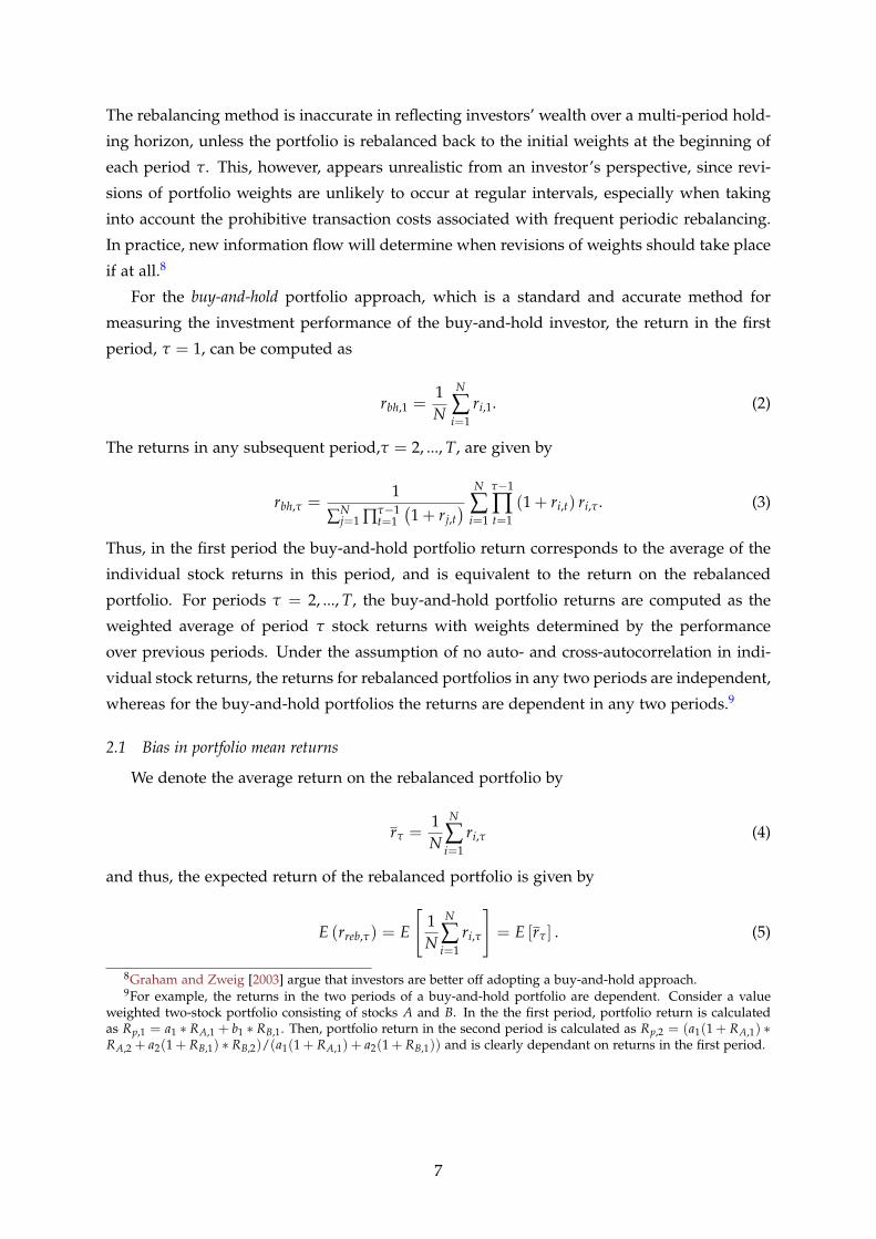
The rebalancing method is inaccurate in reflecting investors’ wealth over a multi-period hold-
ing horizon, unless the portfolio is rebalanced back to the initial weights at the beginning of
each period τ. This, however, appears unrealistic from an investor’s perspective, since revi-
sions of portfolio weights are unlikely to occur at regular intervals, especially when taking
into account the prohibitive transaction costs associated with frequent periodic rebalancing.
In practice, new information flow will determine when revisions of weights should take place
if at all.8
For the buy-and-hold portfolio approach, which is a standard and accurate method for
measuring the investment performance of the buy-and-hold investor, the return in the first
period, τ = 1, can be computed as
rbh,1 =1N
N
∑i=1
ri,1. (2)
The returns in any subsequent period,τ = 2, ..., T, are given by
rbh,τ =1
∑Nj=1 ∏τ−1
t=1
(1 + rj,t
) N
∑i=1
τ−1
∏t=1
(1 + ri,t) ri,τ. (3)
Thus, in the first period the buy-and-hold portfolio return corresponds to the average of the
individual stock returns in this period, and is equivalent to the return on the rebalanced
portfolio. For periods τ = 2, ..., T, the buy-and-hold portfolio returns are computed as the
weighted average of period τ stock returns with weights determined by the performance
over previous periods. Under the assumption of no auto- and cross-autocorrelation in indi-
vidual stock returns, the returns for rebalanced portfolios in any two periods are independent,
whereas for the buy-and-hold portfolios the returns are dependent in any two periods.9
2.1 Bias in portfolio mean returns
We denote the average return on the rebalanced portfolio by
rτ =1N
N
∑i=1
ri,τ (4)
and thus, the expected return of the rebalanced portfolio is given by
E (rreb,τ) = E
[1N
N
∑i=1
ri,τ
]= E [rτ] . (5)
8Graham and Zweig [2003] argue that investors are better off adopting a buy-and-hold approach.9For example, the returns in the two periods of a buy-and-hold portfolio are dependent. Consider a value
weighted two-stock portfolio consisting of stocks A and B. In the the first period, portfolio return is calculatedas Rp,1 = a1 ∗ RA,1 + b1 ∗ RB,1. Then, portfolio return in the second period is calculated as Rp,2 = (a1(1 + RA,1) ∗RA,2 + a2(1 + RB,1) ∗ RB,2)/(a1(1 + RA,1) + a2(1 + RB,1)) and is clearly dependant on returns in the first period.
7

First, we derive the return bias for τ = 2, and then generalise it to an arbitrary τ.10 We use the
approximation 1/(1+rτ) ≈ 1− rτ, ignoring higher order terms in the Taylor series expansion.
The bias between the expected return of the rebalanced and the buy-and-hold portfolios is
given by
BiasE2 = E(rreb,2)− E(rbh,2), (6)
and using Eq. (5) and Eq. (3) for τ = 2, we can write
BiasE2 = E [r1r2]−
1N
N
∑i=1
E [(1− r1) ri,1ri,2] . (7)
The result in Eq. (7) has been documented in Liu and Strong [2008], its derivations appear in
Appendix A to make this study self-contained.
Assuming that r1 is uncorrelated with individual returns ri,1 and ri,2, as proposed in Liu
and Strong [2008], Eq. (7) can further be decomposed as
BiasE2 = E(r1)E(r2) + Cov(r1,r2)︸ ︷︷ ︸
>0
− E (1− r1)︸ ︷︷ ︸>0
1N
N
∑i=1
E(ri,1)E(ri,2)
+
− E (1− r1)︸ ︷︷ ︸>0
1N
N
∑i=1
Cov(ri,1, ri,2)︸ ︷︷ ︸<0
.
︸ ︷︷ ︸>0
(8)
Eq. (8) indicates that even if returns are independent, the return bias is non-zero. The bias
depends on the expected average portfolio return of the rebalanced portfolio, expected in-
dividual stock returns, the autocovariance of the portfolio returns and autocovariances of
individual stock returns. Following the empirical evidence documented in Lo and Mackinlay
[1990] and Mech [1993], portfolio returns are positively autocorrelated, that is, Cov(r1,r2) > 0
for the rebalanced portfolio, contributing positively to a bias.11 Conversely, individual re-
turns are negatively autocorrelated, that is, Cov(ri,1, ri,2) < 0, see Fisher [1966], Roll [1984],
Lo and Mackinlay [1990], Jegadeesh and Titman [1995].12 This negative autocorrelation is
more pronounced in small and low-price stocks, see Lo and Mackinlay [1990]. Hence, in
portfolios comprised of small and low-price stocks, one would expect to observe a positive
bias.13 On the other hand, Kaul and Nimalendran [1990] document positive autocorrelation10We note that there is no bias if the holding period corresponds to a single period (τ = 1). However, one
would not consider an investment strategy based on a single period as it is unattractive due to transaction costs;or simply not adequate for constructing a sufficient sample of decomposed portfolio returns for testing assetpricing models.
11In fact, transaction costs cause the portfolio return autocorrelation by delaying price adjustment.12The negative autocorrelation in individual returns is caused by nonsynchronous trading (Fisher, 1966), trans-
action costs and bid-ask spreads (Roll, 1984, Jegadeesh and Titman, 1995).13For instance, Liu [2006] documents high correlation between the returns of infrequently traded stocks and size,
8

between stock returns once the bid-ask spread is extracted; which may lead to negative bias
in portfolios comprised of large and high-price stocks.
Using Eq. (3) and Eq. (5), we can express the bias in portfolio mean returns for τ = 2, ..., T
as
BiasEτ = E(rreb,τ)− E(rbh,τ) (9)
=N
∑i=1
[1N
E(ri,τ)− E
(1
∑Nj=1 ∏τ−1
t=1
(1 + rj,t
) N
∑i=1
τ−1
∏t=1
(1 + ri,t) ri,τ
)].
Generalising the discussion above to an arbitrary τ, we concur that positive bias in portfolio
mean returns is most likely to occur in small and low-price stock portfolios, and negative bias
is expected in large and high-price stock portfolios. Liu and Strong [2008] note that negative
bias can arise when expected stock returns are constant over time but vary cross-sectionally,
that is, when high (low) expected returns are associated with higher (lower) expected weights
in the buy-and-hold portfolios (second term of Eq. (9)). Rebalancing reverses this effect (first
term of Eq. (9)).
The two approximations employed by Liu and Strong [2008] to arrive at a closed form
solution in Eq. (7) are restrictive. It is well- known that the distribution of individual securities
is negatively skewed. As a result, this approximation may not be valid. In our empirical
analysis we avoid using the closed form solution and rely on real data with no assumptions
on return distributions.14
2.2 Bias in portfolio variance
Similar to the computation of the bias in portfolio mean returns, we derive bias in port-
folio variance for τ = 2, and generalise it to an arbitrary τ. The variance bias between the
rebalanced and the buy-and-hold portfolio is given by
BiasV2 = Var(rreb,2)−Var(rbh,2), (10)
where the variance of the rebalanced portfolio is determined by
Var(rreb,2) = Var [r2] = E[r2
2]− E [r2]
2 , (11)
and the variance of the buy-and-hold portfolio can be written (see Appendix A for details) as
as well as the bid-ask spread; and Branch and Freed [1977], Conrad and Kaul [1993] find a negative relationshipbetween price and the bid-ask spread.
14The following result employs the second order Taylor expansion around zero: 1/(1 + r) ≈ 1 − r + r2 forr → 0. Using daily return data for the S&P500 constituents, we estimate, on average, less than 0.01% differencebetween approximations using the first vs the second order Taylor series.
9
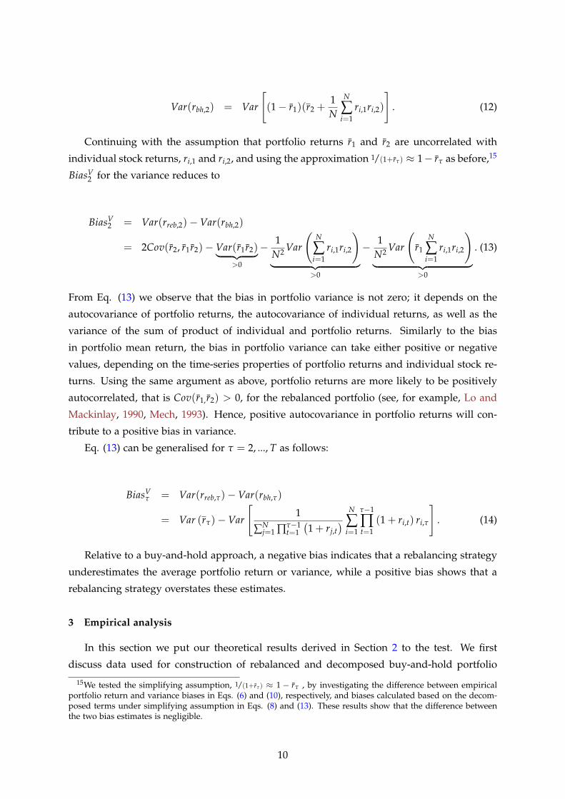
Var(rbh,2) = Var
[(1− r1)(r2 +
1N
N
∑i=1
ri,1ri,2)
]. (12)
Continuing with the assumption that portfolio returns r1 and r2 are uncorrelated with
individual stock returns, ri,1 and ri,2, and using the approximation 1/(1+rτ) ≈ 1− rτ as before,15
BiasV2 for the variance reduces to
BiasV2 = Var(rreb,2)−Var(rbh,2)
= 2Cov(r2, r1r2)−Var(r1r2)︸ ︷︷ ︸>0
− 1N2 Var
(N
∑i=1
ri,1ri,2
)︸ ︷︷ ︸
>0
− 1N2 Var
(r1
N
∑i=1
ri,1ri,2
)︸ ︷︷ ︸
>0
. (13)
From Eq. (13) we observe that the bias in portfolio variance is not zero; it depends on the
autocovariance of portfolio returns, the autocovariance of individual returns, as well as the
variance of the sum of product of individual and portfolio returns. Similarly to the bias
in portfolio mean return, the bias in portfolio variance can take either positive or negative
values, depending on the time-series properties of portfolio returns and individual stock re-
turns. Using the same argument as above, portfolio returns are more likely to be positively
autocorrelated, that is Cov(r1,r2) > 0, for the rebalanced portfolio (see, for example, Lo and
Mackinlay, 1990, Mech, 1993). Hence, positive autocovariance in portfolio returns will con-
tribute to a positive bias in variance.
Eq. (13) can be generalised for τ = 2, ..., T as follows:
BiasVτ = Var(rreb,τ)−Var(rbh,τ)
= Var (rτ)−Var
[1
∑Nj=1 ∏τ−1
t=1
(1 + rj,t
) N
∑i=1
τ−1
∏t=1
(1 + ri,t) ri,τ
]. (14)
Relative to a buy-and-hold approach, a negative bias indicates that a rebalancing strategy
underestimates the average portfolio return or variance, while a positive bias shows that a
rebalancing strategy overstates these estimates.
3 Empirical analysis
In this section we put our theoretical results derived in Section 2 to the test. We first
discuss data used for construction of rebalanced and decomposed buy-and-hold portfolio
15We tested the simplifying assumption, 1/(1+rτ) ≈ 1− rτ , by investigating the difference between empiricalportfolio return and variance biases in Eqs. (6) and (10), respectively, and biases calculated based on the decom-posed terms under simplifying assumption in Eqs. (8) and (13). These results show that the difference betweenthe two bias estimates is negligible.
10

returns, followed by the estimation methodology, results and implications for portfolio con-
struction and investment decisions.
3.1 Data
We construct equally weighted rebalanced and buy-and-hold portfolios of various sizes
from S&P 500 constituents over a nine-year sample period from January 2, 2003 to December
30, 2011. We let the number of stocks in each portfolio vary between 1 and 80, and select
stocks randomly without replacement. The period under consideration includes the global
financial crisis (GFC) associated with the bankruptcy of Lehman Brothers in September 2008
and the subsequent period of turmoil in the U.S. and international financial markets. The un-
derlying data are 5 minute, daily, weekly and monthly observations on prices for 501 stocks
drawn from the constituent list of the S&P 500 index during the sample period, obtained from
SIRCA Thompson Reuters Tick History. This data set was constructed by Dungey et al. [2012]
and does not contain all the stocks listed in the S&P 500 index, but has drawn from that pop-
ulation to select those with sufficient coverage and data availability for high frequency time
series analysis. The original dataset of over 900 stocks was taken from the 0#.SPX mnemonic
provided by SIRCA. This included several stocks that were traded OTC and on alternative
exchanges. The stocks that changed the currency in which they were traded during the period
under consideration were excluded from the analysis. We adjusted the dataset for changes
in RIC codes16 resulted from mergers and acquisitions, stock splits and trading halts. We
removed stocks with insufficient number of observations. We force the inclusion of Lehman
Brothers until their bankruptcy in September 2008, but drop Fannie Mae and Freddie Mac
from the analysis. The data handling process is documented in the web-appendix to Dungey
et al. [2012]. The final data set contains 501 individual stocks. Our estimation methods are
summarised in the next subsection and detailed in Appendix B. The full list of stocks includ-
ing Reuters Identification Codes (RICs) is provided in the supplementary online appendix.
3.2 Estimation method and results
We allow for the diversification effect in portfolios, that is, the relationship between the
decreasing risk in portfolios when the number of securities in these portfolios increases.17
Figure 2 represents the variance bias in portfolios by year (2003-2011).18 To calculate biases,
for each simulated portfolio, we retain the same draw of stocks from the S&P 500 constituents
list when contrasting rebalanced and buy-and-hold approaches.19 The number of stocks,
16A Reuters instrument code, or RIC, is a ticker-like code used by Thomson Reuters to identify financial instru-ments and indices.
17We note that one can obtain most of the benefits of diversification by holding a relatively small number ofstocks; see, e.g., Elton and Gruber [1977].
18In the finance literature, measuring risk is more contentious than measuring return. With different samplingfrequencies, our risk measures, even when annualised, may differ. To help in our comparison of biases in port-folio variance across different data sampling frequencies, we find it practical to focus on relative measures forpresentation purposes, and define bias in portfolio variance in our empirical section as BiasV/Var(rbh).
19Our results demonstrate significant biases when considering a sample of large stocks from the S&P 500 index.As documented in Liu and Strong [2008, p.2245], one would expect to observe even more significant results whenconsidering low-price, small, and loser stocks.
11

Figu
re2:
Var
ia
nc
eBi
as
in
po
rt
fo
lio
sb
yy
ea
r.
Var
ianc
ebi
as(m
ean,
med
ian
and
confi
denc
eba
nds)
for
the
reba
lanc
edvs
.th
ebu
y-an
d-ho
ldpo
rtfo
lioby
year
(200
3-20
11).
The
reba
lanc
ing
ispe
rfor
med
daily
whi
leth
ebu
y-an
d-ho
ldpo
rtfo
lios
are
held
for
one
year
.The
shad
edre
gion
repr
esen
tsth
ear
eabe
twee
nth
e5t
han
dth
e95
thpe
rcen
tile
sof
esti
mat
edbi
ases
for
10,0
00ra
ndom
draw
s.To
cons
truc
tpo
rtfo
lios,
Nst
ocks
are
sele
cted
rand
omly
,whe
reN
=1,
...,8
0an
dth
enu
mbe
rof
poss
ible
dist
inct
port
folio
com
bina
tion
sis
501!
N! (
501−
N)!
,whi
chis
10,0
00fo
ran
y2<
N<
500.
The
port
folio
vari
ance
bias
for
sing
lest
ock
port
folio
sis
alw
ays
zero
and
prov
ides
ana
tura
lsta
rtin
gpo
int.
12

Figure 3: Bias in portfolios at different frequencies.
Variance bias (top panel), average return bias (middle panel) and signal-to-noise ratio bias (bottom panel) acrosstime (left panels) and for the selected year 2008 (right panels). All quantities are constructed based on returnsof randomly selected portfolios of 50 assets using the past one year of data. At the end of each month in theperiod from 2003 to 2011 we obtain portfolio bias estimates using one year of past data (panels on the left). Using5-minute, daily, weekly and monthly sampling frequencies, we estimate variance biases for 2008 across randomlyselected portfolios of sizes N = 1, ..., 80 stocks (panels on the right). The rebalancing is performed depending onthe frequency being analysed while the buy-and-hold portfolios are held for one year either in a rolling window(left panels) or a single exemplar year (right panels). The shaded region represents the area between the 5thand the 95th percentile of estimated daily biases for 10,000 random draws. To construct portfolios, N stocks areselected randomly, where 501!
N!(501−N)! 10, 000. We use the same dataset but sample at different frequencies. Wekeep the same sample of assets in each simulated portfolio across estimations for different frequencies. Overnightreturns for the 5-minute data have been included.
N = 1, ..., 80, is shown on the x-axis.20 Stocks in the simulated portfolios are chosen randomly
20The portfolio variance bias for a single stock portfolio is always zero and provides a natural starting point inthe Figure.
13
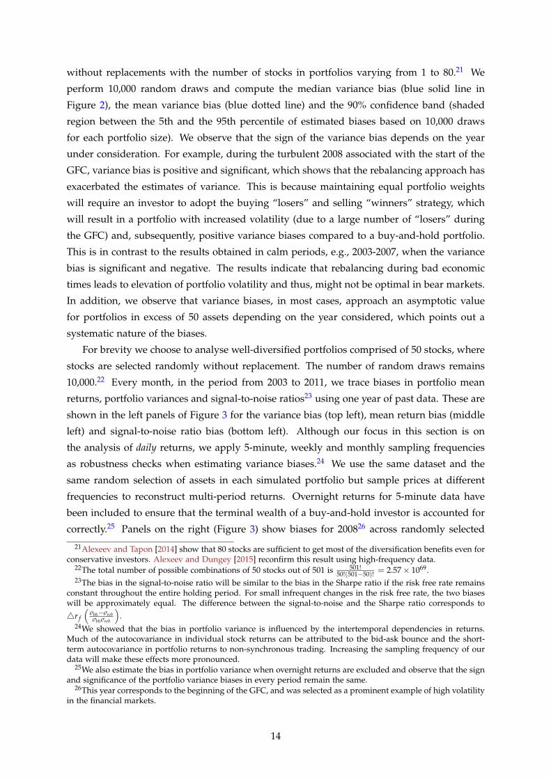
without replacements with the number of stocks in portfolios varying from 1 to 80.21 We
perform 10,000 random draws and compute the median variance bias (blue solid line in
Figure 2), the mean variance bias (blue dotted line) and the 90% confidence band (shaded
region between the 5th and the 95th percentile of estimated biases based on 10,000 draws
for each portfolio size). We observe that the sign of the variance bias depends on the year
under consideration. For example, during the turbulent 2008 associated with the start of the
GFC, variance bias is positive and significant, which shows that the rebalancing approach has
exacerbated the estimates of variance. This is because maintaining equal portfolio weights
will require an investor to adopt the buying “losers” and selling “winners” strategy, which
will result in a portfolio with increased volatility (due to a large number of “losers” during
the GFC) and, subsequently, positive variance biases compared to a buy-and-hold portfolio.
This is in contrast to the results obtained in calm periods, e.g., 2003-2007, when the variance
bias is significant and negative. The results indicate that rebalancing during bad economic
times leads to elevation of portfolio volatility and thus, might not be optimal in bear markets.
In addition, we observe that variance biases, in most cases, approach an asymptotic value
for portfolios in excess of 50 assets depending on the year considered, which points out a
systematic nature of the biases.
For brevity we choose to analyse well-diversified portfolios comprised of 50 stocks, where
stocks are selected randomly without replacement. The number of random draws remains
10,000.22 Every month, in the period from 2003 to 2011, we trace biases in portfolio mean
returns, portfolio variances and signal-to-noise ratios23 using one year of past data. These are
shown in the left panels of Figure 3 for the variance bias (top left), mean return bias (middle
left) and signal-to-noise ratio bias (bottom left). Although our focus in this section is on
the analysis of daily returns, we apply 5-minute, weekly and monthly sampling frequencies
as robustness checks when estimating variance biases.24 We use the same dataset and the
same random selection of assets in each simulated portfolio but sample prices at different
frequencies to reconstruct multi-period returns. Overnight returns for 5-minute data have
been included to ensure that the terminal wealth of a buy-and-hold investor is accounted for
correctly.25 Panels on the right (Figure 3) show biases for 200826 across randomly selected
21Alexeev and Tapon [2014] show that 80 stocks are sufficient to get most of the diversification benefits even forconservative investors. Alexeev and Dungey [2015] reconfirm this result using high-frequency data.
22The total number of possible combinations of 50 stocks out of 501 is 501!50!(501−50)! = 2.57× 1069.
23The bias in the signal-to-noise ratio will be similar to the bias in the Sharpe ratio if the risk free rate remainsconstant throughout the entire holding period. For small infrequent changes in the risk free rate, the two biaseswill be approximately equal. The difference between the signal-to-noise and the Sharpe ratio corresponds to
4r f
(σbh−σrebσbhσreb
).
24We showed that the bias in portfolio variance is influenced by the intertemporal dependencies in returns.Much of the autocovariance in individual stock returns can be attributed to the bid-ask bounce and the short-term autocovariance in portfolio returns to non-synchronous trading. Increasing the sampling frequency of ourdata will make these effects more pronounced.
25We also estimate the bias in portfolio variance when overnight returns are excluded and observe that the signand significance of the portfolio variance biases in every period remain the same.
26This year corresponds to the beginning of the GFC, and was selected as a prominent example of high volatilityin the financial markets.
14

portfolios of size N = 1, ..., 80 stocks. The shaded region represents the 90% confidence
interval around daily biases. As expected, the higher the frequency of the data, and thus,
the frequency of rebalancing to maintain equal weights in the portfolio, the larger the bias in
returns (middle right panel). Confirming the results reported in Figure 2, we observe from
the left panel of Figure 3 that for portfolios of 50 assets, significant negative biases occur
during 2003, 2005 and 2010. This indicates that rebalancing of portfolios in these years leads
to a lower variance than the buy-and-hold approach, and thus, indicates that the rebalancing
strategy underestimates portfolio variance. Significantly positive biases, occurring in the more
turbulent 2008 and 2011, indicate that the rebalancing strategy overshoots the buy-and-hold
strategy. This confirms our previous results that the rebalancing appears to be a favourable
strategy during good economic conditions, but results in larger portfolio volatility during
economic downturns.
In Table 1 we present a summary of the results for equally weighted rebalanced and buy-
and-hold portfolios, obtained using daily data and 10,000 randomly constructed portfolios of
50 stocks. We assume that from the first trading day of the year the investor either follows a
rebalancing strategy and calculates portfolio returns using Eq. (1), or adheres to a buy-and-
hold strategy using Eq. (3). For each given year we estimate portfolio mean returns (columns
1 and 4), standard deviations (columns 2 and 5) and signal-to-noise ratios27 (columns 3 and
6) based on daily returns within that year. The results are reported in annualised terms.28
For the bias results in columns (7) through (9), “*” denotes significance at 10% significance
level, that is, when the range from the 5th percentile to the 95th percentile of estimated biases
in portfolio statistics for a given year does not contain zero. We emphasise that the bias
statistics are computed based on matched pairs of rebalanced and buy-and-hold portfolio
returns, i.e., for the same draw of stocks in the same period. We compute biases at the end
of a year for each of the 10,000 portfolios, and then average them across these portfolios. We
notice that portfolio mean returns in 2006, and especially in 2008-2009, were overstated by
the rebalancing approach. This overstatement of portfolio returns have been observed in at
least 90% of the 10,000 randomly constructed portfolios. On the other hand, the variance
has been significantly understated in 2003, 2005, and 2010. The largest bias in portfolio
variance has occurred in 2008, with another significant exaggeration in 2011. This confirms
our previous results from Figure 2 and Figure 3. The overstatement of the signal-to-noise ratio
by the rebalancing strategy occurred in 2003, 2006, 2008 and 2009. Table 2 reports the ten
largest positive (negative) biases in portfolio mean returns and portfolio variances in panel
A (panel B). We observe that the largest significant biases in portfolio mean returns occur
during the most turbulent 2008-2009, confirming previous results. The results for the largest
significant biases in portfolio variance are mixed; however 6 out of 9 significant biases occur
27We avoid the sample size bias in the signal-to-noise ratio discussed in Miller and Gehr [1978] since the numberof observations is the same for both the buy-and-hold and the rebalanced portfolios in each simulation.
28Daily estimates have been annualised using a factor of 250 for mean returns, and√
250 for standard deviationand signal-to-noise ratio.
15

Tabl
e1:
Me
an
po
rt
fo
lio
re
tu
rn
,va
ria
nc
ea
nd
sig
na
l-t
o-n
oise
ra
tio
fo
rr
eb
al
an
ce
da
nd
bu
y-a
nd
-ho
ld
po
rt
fo
lio
su
sin
gd
aily
da
ta
.
Reb
alan
ced
port
folio
Buy-
and-
hold
port
folio
Bias
(1)
(2)
(3)
(4)
(5)
(6)
(7)
(8)
(9)
Year
Avg
.ret
urn
(%)
St.D
ev(%
)Si
gnal
-to-
nois
eA
vg.r
etur
n(%
)St
.Dev
(%)
Sign
al-t
o-no
ise
Bia
sEB
iasV
Var(r
bh)
(%)
Bia
sS
2003
33.5
17.3
1.94
33.2
17.9
1.85
0.36
-6.9
7*0.
09*
2004
16.3
13.2
1.24
15.6
13.2
1.18
0.66
-0.8
70.
0620
057.
212
.20.
596.
212
.50.
490.
97-4
.26*
0.09
2006
12.6
12.4
1.02
11.1
12.4
0.90
1.43
*-0
.99
0.12
*20
072.
917
.00.
174.
817
.10.
28-1
.85
-1.1
0-0
.10
2008
-36.
145
.1-0
.80
-41.
641
.8-0
.99
5.43
*16
.35*
0.19
*20
0948
.935
.51.
3845
.334
.81.
303.
57*
3.72
0.08
*20
1021
.021
.30.
9920
.521
.60.
950.
51-2
.88*
0.04
2011
-1.3
27.3
-0.0
4-1
.826
.3-0
.07
0.48
8.43
*0.
02U
sing
daily
freq
uenc
y,w
eco
mpu
tean
nual
ised
aver
ages
ofpo
rtfo
liore
turn
s(c
olum
ns1
and
4),
stan
dard
devi
atio
n(c
olum
ns2
and
5)an
dsi
gnal
-to-
nois
era
tios
(col
umns
3an
d6)
base
don
10,0
00ra
ndom
lyco
nstr
ucte
dpo
rtfo
lios
of50
stoc
ksth
atar
eeq
ually
wei
ghte
dat
the
begi
nnin
gof
each
year
.Th
ere
bala
ncin
gis
perf
orm
edda
ilyw
hile
the
buy-
and-
hold
port
folio
sar
ehe
ldfo
ron
eye
ar.
Dai
lyes
tim
ates
have
been
annu
alis
edus
ing
afa
ctor
of25
0fo
rav
erag
ere
turn
s;√
250
for
stan
dard
devi
atio
nan
dsi
gnal
-to-
nois
era
tio.
For
the
bias
inav
erag
epo
rtfo
liore
turn
s(c
olum
ns7)
,por
tfol
iova
rian
ce(c
olum
n8)
,and
sign
al-t
o-no
ise
rati
o(c
olum
n9)
,“*”
deno
tes
sign
ifica
nce
at10
%si
gnifi
canc
ele
vel.
For
pres
enta
tion
purp
oses
,bia
sin
vari
ance
(col
umn
8)is
pres
ente
das
ape
rcen
tage
.
16

Figure 4: Bias Decomposition.
2004 2005 2006 2007 2008 2009 2010 2011
−5
0
5
10
x 10−5 Return Bias Decomposition
Period
Term 1Term 2Term 3Term 4Bias in Portfolio Returns
2004 2005 2006 2007 2008 2009 2010 2011
−2
−1
0
1
2
3
4
5
x 10−6 Variance Bias Decomposition
Period
Term 1Term 2Term 3Term 4Bias in Portfolio Variance
Return bias decomposition BiasE2 derived in Eq. (8) (left panel) and variance
bias decomposition BiasV2 derived in Eq. (13) (right panel). Namely, BiasE
2 =
E(r1)E(r2)︸ ︷︷ ︸Term 1
+Cov(r1,r2)︸ ︷︷ ︸Term 2
−E (1− r1)1N
N
∑i=1
E(ri,1)E(ri,2)︸ ︷︷ ︸Term 3
−E (1− r1)1N
N
∑i=1
Cov(ri,1, ri,2)︸ ︷︷ ︸Term 4
and BiasV2 =
2 Cov(r2, r1r2)︸ ︷︷ ︸Term 1
−Var(r1r2)︸ ︷︷ ︸Term 2
− 1N2 Var
(N
∑i=1
ri,1ri,2
)︸ ︷︷ ︸
Term 3
− 1N2 Var
(r1
N
∑i=1
ri,1ri,2
)︸ ︷︷ ︸
Term 4
. Portfolios are constructed from
randomly selected 50 assets. At the end of each month, in the period from 2003 to 2011, the bias estimates andthe decomposed terms were obtained using one year of past data. Thus, the rebalancing is performed dailywhile the buy-and-hold portfolios are held for one year. Decomposed terms and biases are the averages of 10,000randomly drawn portfolios each with 50 assets.
between November 2007 and August 2011. This period corresponds to the turbulent period
of the financial crisis, followed by the global recession. We confirm previous results that the
rebalancing method exacerbates expected returns and variances of buy-and-hold portfolios
during that period. The results for the lowest biases indicate that none of the return biases are
significant at the 90% level; however all the portfolio variance biases are significant, with the
largest significant biases occurring in 2009. Our results indicate that researchers and portfolio
managers may mistakenly measure portfolio performance when relying only on biases for
the portfolio mean returns while ignoring second moments. This is especially pertinent for
the situation at hand: although biases in portfolio mean returns appear insignificant due
to increased volatility, biases in the variance of portfolios are significant for all years under
consideration. Liu and Strong [2008] and Canina et al. [1998] discuss common time-series
characteristics of both the portfolio and individual stocks returns and the implication that
these characteristics may exhibit on the portfolio return bias. However, Canina et al. [1998]
do not derive the portfolio mean return bias but instead use regression analysis to explain the
bias using a set of time-series characteristics of the underlying portfolios and stocks. They
calculate the cross-sectional average autocorrelations of each stock, the autocorrelations for
the equally weighted rebalanced portfolio, and the cross-sectional variance of the average
returns. Lo and Mackinlay [1990] document that average daily autocorrelations in returns are
mostly negative. The empirical literature shows that individual stock returns are negatively
17

Table 2: 20 largest biases.
Rank Year Month BiasE Rank Year Month BiasV
Var(rbh)(%)
Panel A: Months with highest bias1 2008 October 15.84* 1 2008 November 8.51*2 2009 March 13.17* 2 2008 October 7.51*3 2008 November 11.36* 3 2009 January 4.47*4 2008 December 6.31 4 2006 July 4.40*5 2008 September 4.29 5 2009 February 4.20*6 2008 July 3.49* 6 2004 July 4.01*7 2009 February 3.27 7 2008 September 3.808 2009 May 3.06 8 2006 June 3.32*9 2008 January 3.02 9 2011 August 3.15*
10 2009 January 2.91 10 2007 November 2.93*
Panel B: Months with lowest bias108 2009 April -4.47 108 2009 April -10.53*107 2008 June -2.63 107 2009 May -5.53*106 2009 August -2.36 106 2009 August -4.91*105 2011 September -1.68 105 2004 January -3.57*104 2006 January -0.89 104 2008 August -3.26*103 2003 April -0.81 103 2003 August -3.16*102 2003 May -0.79 102 2003 October -2.83*101 2009 December -0.75 101 2010 April -2.34*100 2007 December -0.74 100 2003 July -2.29*99 2004 April -0.70 99 2011 October -2.29*
The largest positive (negative) biases in portfolio returns and portfolio variances are reported in panel A (panelB). At the end of each month in the period from 2003 to 2011 we obtain portfolio bias estimates using one monthof past data. The rebalancing is performed daily while the buy-and-hold portfolios are held for one month. Weobserve that the largest significant biases in portfolio returns occur during the turbulent years 2008-2009. Theresults for the largest significant biases in portfolio variance are mixed; however 6 out of 9 significant biases occurbetween November 2007 and August 2011. “*” denotes significance at 10% significance level, that is, when therange from the 5th percentile to the 95th percentile of estimated biases in portfolio statistics for a given year doesnot contain zero. For presentation purposes, bias in variance is presented as a percentage.
autocorrelated because of non-synchronous trading (e.g., Fisher [1966]) or bid-ask spreads
(e.g., Roll [1984], Jegadeesh and Titman [1995]). Our evidence precludes us from drawing the
same conclusion. Given that our sample comprises the largest 501 stocks in the U.S. financial
markets, non-synchronous trading or bid-ask spreads might not be an issue, at least for daily
or lower frequencies. Consistent with the previous literature (Lo and Mackinlay [1990], Mech
[1993], Canina et al. [1998]) we observe, on average, positive first-order autocorrelations29 in
portfolios for the first half of our sample.30 However, following the financial crisis associated
with the bankruptcy of Lehman Brothers in September 2008 and the subsequent period of
turmoil in the U.S., we observe negative first-order autocorrelations in portfolio returns. The
second- and third-order autocorrelations in portfolios are negative on average, which is in
29The results for autocorrelations are not reported here, but are available from the authors upon request.30Transaction costs cause portfolio returns to be autocorrelated by delaying price adjustment.
18

line with the results reported in Canina et al. [1998]. The cross-sectional variance of average
returns is stable for the first half of our sample, and becomes volatile starting from 2007,
which corresponds to the start of the GFC and subsequent period of global recession.
Figure 4 shows bias in the portfolio mean return, BiasE, and bias in the portfolio variance,
BiasV , respectively, decomposed into its components as defined by Eq. (8) and Eq. (13). The
terms that impact the mean return bias (left panel) include the autocovariance of average
portfolio returns (Term 2, red line) and the term involving autocovariance of individual stock
returns (Term 4, yellow line). In contrast, average portfolio returns (Term 1, blue line) and the
term involving average individual stock returns (Term 3, green line) are negligible. The terms
that impact bias in portfolio variance (right panel) include the covariance between the average
portfolio returns r2 and the product r1r2 (Term 1, blue line), the variance of the product of
portfolio returns r1r2 (Term 2, red line) and the term that depends on the variance of the
sum of the product of individual stock returns ∑Ni=1 ri,1ri,2 (Term 3, green line). Conversely,
the variance of the product of the average portfolio return and the sum of individual returns
r1 ∑Ni=1 ri,1ri,2 (Term 4, yellow line) can be neglected.
Transactions costs have important implications for the bias in portfolio mean returns, con-
sidering the amount of trading involved in the case of rebalanced portfolios. Liu and Strong
[2008] discuss this issue and document four alternative estimates of transactions costs. In
fact, from Eq. (8) we can directly observe the relationship between bias in the portfolio mean
return and expected returns on both the portfolio and individual stocks. On the contrary, the
portfolio variance bias in Eq. (13) relies solely on variances of the portfolio and individual
stock returns, as well as intertemporal dependencies in these returns, with transactions costs
having minimal influence on the bias.
In the next section we demonstrate that the optimal portfolio size required to obtain a
well-diversified portfolio is heavily reliant on portfolio construction method especially for
longer investment horizons.
4 Implications for Portfolio Analysis
In this section, we examine the implications variance bias can have for factor model in-
ference as well as optimal portfolio size recommendations in achieving target diversification
levels.
4.1 Factor models inference
In considering the implications of variance bias on inference in factor models we rely on
the four-factor model of Carhart [1997]. We regress daily returns of simulated rebalanced
and buy-and-hold portfolios on the asset pricing model common factors taken each year and
over the period from 2003 to 2011.31 Our simulated portfolios are constructed from 50 assets
31The Fama-French data and momentum factor source is Kenneth French’s web site at Dartmouth, see https://mba.tuck.dartmouth.edu/pages/faculty/ken.french/data_library.html.
19

Figure 5: Bias in Factor model estimates.
We contrast the factor model estimates and inference statistic of portfolios based on rebalanced strategy with theresults from buy-and-hold approach. Left panels depict difference in estimated coefficients. Right panels showdifference in t-statistic. The rebalancing is performed daily while the buy-and-hold portfolios are held for oneyear (the top and middle panels) or for the entire period (the bottom panel).
drawn 10,000 times without replacement keeping the selection identical for the rebalanced
and buy-and-hold portfolios at each draw. We perform two sets of regressions using
rk,t = ai + bi MKTt + ciSMBt + di HMLt + eiUMDt + ε it, (15)
where rk,t is the return in excess of the one-month Treasury bill rate on the rebalanced
20

(k = reb) and buy-and-hold (k = bh) portfolios. MKT is the excess return on the value-
weighted aggregate market proxy; and SMB, HML, and UMD are returns on value-weighted,
zero-investment, factor-mimicking portfolios for size, book-to-market equity, and one-year
momentum in stock returns.
Figure 5 shows differences in estimated coefficients (left panels) and corresponding t-
statistics (right panels) for years 2006 (top panels) and 2008 (middle panels) as well as for the
entire period (bottom panels). Earlier, in Figure 2, we identified years 2006 and 2008 as the
periods of the least and the most bias in portfolio variances when rebalanced portfolios are
contrasted with buy-and-hold portfolios. Our results indicate that UMD is the most affected
factor in terms of the difference in the estimated coefficients as well as the difference in its
significance. We summarise the results of all single-year periods as well as the entire period
in Table 3.32 As expected, MKT, a highly significant variable with the average t-statistic of
65-70, showed no difference in proportion of significant estimates in our simulations. Other
factors proved to be more susceptible to changes in the rebalancing assumption. The results
in Table 3 indicate that UMD factor exhibits the largest change in the number of significant
estimates, making it the prime candidate for spurious inference in four-factor models.
4.2 Portfolio diversification
For convenience, fixed weight strategy is often employed when calculating portfolio re-
turns, inadvertently matching the portfolio rebalancing frequency with that of available data.
If the data are daily, such frequent rebalancing may not be viable or grossly misrepresent the
actual strategy implemented, resulting in wrong inference. We wish to emphasize, however,
that the purpose of this study is not to advocate the use of rebalancing or buy-and-hold port-
folio strategy, but merely to use these two extreme cases to assess and contrast the variance
of portfolio returns based on these two distinct strategies.
In this section, we discuss the importance of the variance biases in determining the op-
timal number of holdings in well-diversified portfolios. We investigate the consequences of
adopting fixed weight and buy-and-hold strategies, in regards to systematic risk assessment,
portfolio diversification and market regime under consideration (relatively calm periods such
as 2003 vs. more turbulent times such as during the 2008 financial crisis). Previous liter-
ature often employs a simplified portfolio return decomposition, involving rebalancing the
portfolio at the beginning of each time period back to the initial weights (see, Evans and
Archer, 1968, Wagner and Lau, 1971, Tang, 2004, Kryzanowski and Singh, 2010, Chong and
Phillips, 2013, among others). These studies underestimate the number of stocks required to
achieve a certain level of portfolio diversification in buy-and-hold portfolios. Intuitively, this
can be inferred from Figure 1 where a buy-and-hold portfolio initially comprised of 10 stocks,
eventually resembles characteristics of a two-stock portfolio. In this section, using portfolio
simulation we investigate the optimal size of portfolios based on the two approaches: fixed
32We include Figure 7 in the appendix where we used 2008 as an exemplar year to showcase our estimationprocedure in more detail.
21

Tabl
e3:
Pro
po
rt
io
no
fsig
nific
an
tfa
ct
or
est
im
at
es
(at
5%si
gnifi
canc
ele
vel)
.
Year
Reb
alan
ced
port
folio
sBu
y-an
d-H
old
port
folio
sD
iffer
ence
αM
KT
SMB
HM
LU
MD
αM
KT
SMB
HM
LU
MD
αM
KT
SMB
HM
LU
MD
2003
0.00
1.00
0.90
0.91
0.57
0.01
1.00
0.96
0.88
0.15
-0.0
10.
00-0
.07
0.03
0.41
2004
0.12
1.00
0.68
0.42
0.54
0.09
1.00
0.59
0.40
0.79
0.03
0.00
0.10
0.02
-0.2
520
050.
031.
000.
810.
220.
610.
021.
000.
660.
170.
770.
010.
000.
150.
06-0
.16
2006
0.07
1.00
0.78
0.09
0.56
0.04
1.00
0.74
0.08
0.65
0.03
0.00
0.04
0.01
-0.0
920
070.
041.
000.
530.
410.
440.
041.
000.
450.
300.
690.
000.
000.
090.
11-0
.25
2008
0.06
1.00
0.89
0.55
0.96
0.00
1.00
0.93
0.49
0.72
0.06
0.00
-0.0
40.
070.
2420
090.
061.
000.
900.
521.
000.
021.
000.
980.
400.
990.
040.
00-0
.08
0.13
0.01
2010
0.03
1.00
0.71
0.55
0.51
0.01
1.00
0.76
0.56
0.66
0.02
0.00
-0.0
5-0
.02
-0.1
620
110.
101.
000.
800.
390.
730.
211.
000.
630.
360.
24-0
.11
0.00
0.17
0.03
0.50
2003
-201
10.
381.
001.
000.
860.
980.
071.
000.
960.
630.
660.
310.
000.
040.
230.
32U
sing
daily
retu
rns
inEq
.(1
5),
we
calc
ulat
epr
opor
tion
sof
sign
ifica
ntes
tim
ates
(at
5%le
vel)
usin
gre
turn
son
10,0
00ra
ndom
lyco
nstr
ucte
dpo
rtfo
lios
of50
stoc
ksth
atar
eeq
ually
wei
ghte
dat
the
begi
nnin
gof
each
peri
odre
port
edin
the
tabl
e.Fo
rth
efix
ed-w
eigh
tpo
rtfo
lios,
reba
lanc
ing
ispe
rfor
med
daily
,mat
chin
gth
efr
eque
ncy
ofth
eda
ta.
As
befo
re,w
em
aint
ain
the
sam
est
ock
sele
ctio
nin
each
rand
omdr
awto
ensu
reth
atth
eon
lydi
ffer
ence
betw
een
reba
lanc
edan
dbu
y-an
d-ho
ldpo
rtfo
lios
isdu
eto
the
reba
lanc
ing
assu
mpt
ion.
We
high
light
edth
ela
rges
tab
solu
tedi
ffer
ence
inpr
opor
tion
ofsi
gnifi
cant
coef
ficie
nts
inbo
ldfo
nt.
22

weight and buy-and-hold strategies.
We document that different number of holdings are required to reach a certain level of
portfolio diversification. While fixed weight portfolio will maintain its diversification po-
tential throughout a period, the buy-and-hold portfolio will start to diverge over time. Our
analysis in Section 3 highlights that the portfolio risk does depend on the rebalancing strategy
and may vary substantially in certain periods.
Figure 6 shows the reduction in diversifiable risk as the number of holdings in a portfolio
increases. We perform the analysis year-by-year (relatively calm period of 2003 and a more
turbulent 2008 year are used as exemplar periods and are included in the top and middle
panels, respectively) and over the entire period (bottom panel). In the left panels of Figure
6 the vertical axis depicts portfolio risk measured by the annualised standard deviation, σn
where n = 1, ..., N.33
Based on Alexeev and Dungey [2015], we define a normalised risk measure that takes
values between zero, for fully diversified portfolios, and one, for single-stock portfolios, as
Ωn =σn − σN
σ1 − σN,
where σ1 represents a single-stock portfolio risk, σN is the market risk computed using all
N stocks. The results reported in Figure 6 (panels on the right) demonstrate that different
number of stocks is required depending on the time period and rebalancing assumption. As
it is evident from the figure, the number of portfolio holdings differ under the two scen-
arios, pointing the fact that the two investment assumptions should be considered carefully.
Although the difference in the number of stocks required to achieve diversification appears
insignificant when comparing fixed weight and buy-and-hold strategies in individual years
(top and middle panels), this difference becomes highly pronounced when investigating the
entire period (bottom panel). In contrast to previous literature that employs fixed weight
approach and suggests that between 10 and 15 stocks are enough to provide adequate diver-
sification, we find that when buy-and-hold strategy is assumed the recommended number
of stocks is substantially higher. For example, during the 2003-2011 period, to achieve 90%
diversification using fixed weight strategy, investors would hold 13 stocks, while for investors
adopting a buy-and-hold approach the required number of stocks increases to 26. This result
reconfirms our findings that researchers and practitioners should take care in implementing
the precise rebalancing strategy when calculating portfolio returns. Overall, one would ex-
pect that the longer the period under consideration the larger the difference in the number of
stocks required will be to achieve diversification under the two rebalancing strategies. Altern-
atively, for the same investment horizon, the larger the discrepancy between data frequency
employed in constructing decomposed portfolio returns and the frequency of the rebalancing
used to construct portfolios, the larger will be the difference in recommended number of
holdings to achieve same levels of portfolio diversification.
33Similar figures can be observed in seminal works by Evans and Archer [1968] and Solnik [1974].
23

Figure 6: Bias in optimal portfolio size.
Number of Stocks (n)0 10 20 30 40 50
Standarddeviation
(annual)
0.15
0.2
0.25
0.3
0.35Period: 2003
Rebalanced PortfolioBuy-and-Hold PortfolioRebalanced Market IndexBuy-and-Hold Market Index
Number of Stocks (n)0 10 20 30 40 50
Normalised
stan
darddeviation
0
0.1
0.2
0.3
0.4
0.5
0.6
0.7
0.8
0.9
1Period: 2003
n=15
n=19
Number of Stocks (n)0 10 20 30 40 50
Standarddeviation
(annual)
0.4
0.45
0.5
0.55
0.6
0.65Period: 2008
Rebalanced PortfolioBuy-and-Hold PortfolioRebalanced Market IndexBuy-and-Hold Market Index
Number of Stocks (n)0 10 20 30 40 50
Normalised
stan
darddeviation
0
0.1
0.2
0.3
0.4
0.5
0.6
0.7
0.8
0.9
1Period: 2008
n=12
n=14
Number of Stocks (n)0 10 20 30 40 50
Standarddeviation
(annual)
0.2
0.22
0.24
0.26
0.28
0.3
0.32
0.34
0.36
0.38
0.4Period: 2003-2011
Rebalanced PortfolioBuy-and-Hold PortfolioRebalanced Market IndexBuy-and-Hold Market Index
Number of Stocks (n)0 10 20 30 40 50
Normalised
stan
darddeviation
0
0.1
0.2
0.3
0.4
0.5
0.6
0.7
0.8
0.9
1Period: 2003-2011
n=13
n=26
Left panels depict portfolio risk (σn, solid lines) and the market risk (σN , dotted horizontal lines) against thenumber of portfolio holdings. Diversifiable risk is defined as the difference between portfolio risk σn (solidline) and the market risk σN (dashed horizontal line) for rebalanced (red lines) and buy-and-hold (blue lines)portfolios, σn − σN . Right panels show the portfolio diversifiable risk as a percentage of the total diversifiablerisk, Ωn = (σn − σN)/(σ1 − σN). We contrast the results obtained using rebalanced strategy (red lines) withthe results from buy-and-hold approach (blue lines). The rebalancing is performed daily while the buy-and-holdportfolios are held for one year (the top and middle panels) or for the entire period (the bottom panel). Horizontalgrey lines at 0.2 and 0.1 represent 80% and 90% reduction in diversifiable risk, respectively.
5 Conclusion
Rebalancing is an essential component of the portfolio management process. The assump-
tion of continuous rebalancing, although impractical, has gained popularity among research-
ers due to its simplicity and tractability. Significant biases in portfolio mean returns and
24

portfolio variances arise as a consequence of incorrectly adopting a rebalancing assumption
in estimating multi-period portfolio returns for buy-and-hold investors. Although such mis-
alignments are rare in the finance literature, adaptation of rebalancing frequency matching
that of the underlying data is quite frequent. In analysing bias in decomposed portfolio
mean returns, Liu and Strong [2008] define return bias as the difference between mean re-
turns of portfolios constructed using the rebalanced and buy-and-hold assumptions. They
show that return bias can have detrimental consequences and results in misleading conclu-
sions on momentum profits. Focusing on the second moment of return distributions, we
compute variance bias as the difference between the variance of portfolios constructed using
rebalanced returns and the decomposed buy-and-hold returns. We show that variance bias is
significant and systematic. We demonstrate that the assumption of continuously rebalanced
versus buy-and-hold weights have consequences for the optimal number of portfolio hold-
ings recommendation in diversified portfolios. In light of the evidence on existence of bias in
portfolio mean returns as well as variance, evaluation of portfolio risk-adjusted performance
may be affected.
In our empirical exercise we avoid restrictive assumptions used to derive the closed form
solution and examine biases arising in the means and variances of portfolios using equally
weighted rebalanced and buy-and-hold portfolios of various sizes constructed from S&P 500
constituents over the nine-year sample period ranging from January 2, 2003 to December 30,
2011. Allowing the number of stocks in portfolios to vary between 1 and 80, we find that
the bias in portfolio variance approaches an asymptotic value for portfolios in excess of 50
assets, pointing to a systematic nature of the bias. Our results (the sign of the bias and its
significance) depend on the period under consideration with its specific time-series properties
for both the portfolio returns and the individual stock returns. In particular, we find that
negative variance biases tend to occur during 2003, 2005 and 2010 indicating that rebalancing
of portfolios understates portfolio variances. Significantly positive biases are attributed to
more turbulent 2008 and 2011, indicating that the rebalancing strategy overstates the buy-
and-hold strategy during these times. This result is not surprising since to maintain equal
portfolio weights for stocks in a portfolio at each time, an investor will have to adopt a buying
“losers” and selling “winners” strategy, resulting in a portfolio with elevated volatility and,
subsequently, positive variance biases compared to a buy-and-hold portfolio. We observe the
largest significant biases in portfolio returns between 2007 and 2011, corresponding to the
turbulent period of the GFC, followed by the global recession. The existence of large biases
in the variance of portfolios during adverse economic conditions suggests that rebalancing
might not be an optimal investment strategy in crisis (and perhaps post-crisis) periods, and a
buy-an-hold strategy should be considered as a viable alternative during these times.
When explaining bias in portfolio mean returns and variances, we find that higher cross-
sectional variability in average portfolio returns results in higher biases. Other variables
contributing to the explanation of these biases include autocovariances of average portfolio
25

returns and autocovariances of individual stock returns. Furthermore, when analysing bias
decomposition, we observe that the autocovariance of average portfolio returns and the auto-
covariance of individual stock returns impact the return bias; whereas the bias in portfolio
variance is influenced by the intertemporal dependencies in both the portfolio and individual
stock returns. The purpose of this study is not to advocate the use of rebalancing or buy-and-
hold portfolio strategy, but merely to use these two extreme cases to assess and contrast the
variance of portfolio returns based on these two distinct strategies. While the difference in
some periods is negligible, we show that there are periods where the difference in the vari-
ance of these two strategies is significant and has consequences for factor model inference
and optimal portfolio size recommendations.
Overall, the existence of portfolio variance biases have important implications not only
when evaluating portfolio risk, but also in measuring portfolio performance. In addition,
these variance biases adversely affect statistical inference in factor models. Our results in-
dicate that one should exercise caution and apply correct assumption on portfolio weight
dynamics when dealing with multi-period portfolio returns, as biases in portfolio variances
and portfolio mean returns can lead to spurious results when analysing investment strategies
or testing asset pricing models. We emphasise that researchers might fall into a methodo-
logical trap when observing (possibly insignificant) biases in portfolio returns and ignoring
second moments, that may, in fact, include large biases. The existence of portfolio variance
biases, particularly during the turbulent periods of financial crises and global recessions,
might have important implications when evaluating portfolio risk-adjusted performance. We
show that under the buy-and-hold strategy, the recommended portfolio sizes required for
well-diversified portfolios may be substantially larger than previously recommended in the
finance literature based on results that employ fixed weight portfolio construction approach.
References
D.-H. Ahn, J. Conrad, and R.F. Dittmar. Risk adjustment and trading strategies. Review of
Financial Studies, 16:459–486, 2003.
V. Alexeev and M. Dungey. Equity portfolio diversification with high frequency data. Quant-
itative Finance, 15(7):1205–1215, 2015.
V. Alexeev and F. Tapon. The number of stocks in your portfolio should be larger than you
think: Diversification evidence from five developed markets. Journal of Investment Strategies,
4(1):43–82, 2014.
M. E. Blume and R. F. Stambaugh. Biases in computed returns: An application to the size
effect. Journal of Financial Economics, 12:387–404, 1983.
B. Branch and W. Freed. Bid-ask spreads on the AMEX and Big Board. Journal of Finance, 32:
159–163, 1977.
26

J. Y. Campbell, A. W. Lo, and A. C. MacKinlay. The Econometrics of Financial Markets. Princeton
University Press, 1997.
L. Canina, R. Michaely, R. Thaler, and K. Womack. Caveat compounder: A warning about
using the daily CRSP equal-weighted index to compute long-run excess returns. The Journal
of Finance, 53(1):403–416, 1998.
M. Carhart. On persistence in mutual fund performance. Journal of Finance, 52:57–82, 1997.
L. K. C. Chan, H.-L. Chen, and J. Lakonishok. On mutual fund investment styles. Review of
Financial Studies, 15:1407–1437, 2002.
James Chong and G. Michael Phillips. Portfolio size revisited. Journal of Wealth Management,
15(4):49–60, 2013.
R. B. Cohen, J. D. Coval, and L. Pastor. Judging fund managers by the company they keep.
Journal of Finance, 60:1057–1096, 2005.
J. Conrad and G. Kaul. Long-term market overreaction or biases in computed returns? Journal
of Finance, 48:39–63, 1993.
K. Daniel, M. Grinblatt, and S. Titman. Measuring mutual fund performance with
characteristic-based benchmarks. Journal of Finance, 52:1035–1058, 1997.
V. DeMiguel, L. Garlappi, and R. Uppal. Optimal versus naive diversification: How inefficient
is the 1/N portfolio strategy? Review of Financial Studies, 22:1915–1953, 2009.
K.B. Diether, K.-H. Lee, and I.M. Werner. Short-sale strategies and return predictability. The
Review of Financial Studies, 22:575–607, 2009.
M. Dungey, M. Luciani, and D. Veredas. Ranking Systemically Important Financial Institu-
tions. Working Papers ECARES 2013/130530, ULB – Universite Libre de Bruxelles, 2012.
E. J. Elton and M. J. Gruber. Risk reduction and portfolio size: An analytic solution. Journal
of Business, 50:415–437, 1977.
John L. Evans and Stephen H. Archer. Diversification and the reduction of dispersion: An
empirical analysis. The Journal of Finance, 23(5):pp. 761–767, 1968.
E.F. Fama and K.R. French. Multifactor explanations of asset pricing anomalies. Journal of
Finance, 51:55–84, 1996.
Eugene F. Fama and Kenneth R. French. Value versus growth: The international evidence.
The Journal of Finance, 53(6):1975–1999, 1998.
L. Fisher. Some new stock market indices. Journal of Business, 29:191–225, 1966.
27

B. Graham and J. Zweig. The Intelligent Investor: The Definitive Book on Value Investing. Harper-
Business Essentials, revised 1973 edition edition, 2003.
P. Gray. Stock weighting and nontrading bias in estimated portfolio returns. Accounting and
Finance, 54:467–503, 2014.
K. Hou, G.A. Karolyi, and B-C. Kho. What factors drive global stock returns? Review of
Financial Studies, 24(8):2527–2574, 2011.
W. Huang, Q. Liu, G. Rhee, and L. Zhang. Return reversals, idiosyncratic risk, and expected
returns. Review of Financial Studies, 23(1):147–168, 2010.
N. Jegadeesh and S. Titman. Short horizon return reversals and the bid-ask spread. Journal of
Financial Intermediation, 4:116–132, 1995.
G. Kaul and M. Nimalendran. Price reversals: Bid-ask errors or market overreaction. Journal
of Financial Economics, 28:67–93, 1990.
Lawrence Kryzanowski and Singh Singh. Should minimum portfolio sizes be prescribed for
achieving sufficiently well-diversified equity portfolios? Frontiers in Finance and Economics,
7(2):1–37, 2010.
C. M. C. Lee and B. Swaminathan. Price momentum and trading volume. Journal of Finance,
55:2017–2069, 2000.
W. Liu. A liquidity augmented capital asset pricing model. Journal of Financial Economics, 82:
631–671, 2006.
W. Liu and N. Strong. Biases in decomposing holding-period portfolio returns. The Review of
Financial Studies, 21(5):2243–2274, 2008.
A. W. Lo and A. C. Mackinlay. When are contrarian profits due to stock market overreaction?
Review of Financial Studies, 3:175–205, 1990.
Michael McAleer and Marcelo C. Medeiros. Realized Volatility: A Review. Econometric Re-
views, 27(1-3):10–45, 2008.
T. S. Mech. Portfolio return autocorrelation. Journal of Financial Economics, 34:307–344, 1993.
R.E. Miller and A.K. Gehr. Sample size bias and sharpe’s performance measure: A note.
Journal of Financial and Quantitative Analysis, 13:943–946, 12 1978. ISSN 1756-6916.
S. Nagel. Short sales, institutional investors and the cross-section of stock returns. Journal of
Financial Economics, 78:277–309, 2005.
R. Roll. A simple implicit measure of the effective bid-ask spread in an efficient market.
Journal of Finance, 39:1127–1139, 1984.
28

Bruno H. Solnik. Why not diversify internationally rather than domestically? Financial
Analysts Journal, 30(4):48–54, 1974.
Gordon Y.N. Tang. How efficient is naive portfolio diversification? an educational note.
Omega, 32(2):155 – 160, 2004.
M. Teo and S.-J. Woo. Style effects in the cross-section of stock returns. Journal of Financial
Economics, 74:367–398, 2004.
Wayne H. Wagner and Sheila C. Lau. The effect of diversification on risk. Financial Analysts
Journal, 27(6):pp. 48–53, 1971.
29

Appendix
A. Derivations
Bias in portfolio returns
Using Eq. (5) and Eq. (3) for τ = 2, we can express the bias between the expected return
of the rebalanced and the buy-and-hold portfolio as follows:
BiasE2 = E(rreb,2)− E(rbh,2)
= E [r2]− E
[1
∑Nj=1(1 + rj,1
) N
∑i=1
(1 + ri,1) ri,2
](A.1)
= E [r2]− E
[1
N (1 + r1)
N
∑i=1
ri,2 +N
∑i=1
ri,1ri,2
]
≈ E [r2]− E
[(1− r1)
1N
N
∑i=1
ri,2 +N
∑i=1
ri,1ri,2
]
= E [r2]− E
[1N
N
∑i=1
ri,2 +1N
N
∑i=1
ri,1ri,2 − r11N
N
∑i=1
ri,2 − r11N
N
∑i=1
ri,1ri,2
]
= E [r2]− E
[r2 +
1N
N
∑i=1
ri,1ri,2 − r1r2 − r11N
N
∑i=1
ri,1ri,2
]
= E
[r1r2 − (1− r1)
1N
N
∑i=1
ri,1ri,2
]
= E [r1r2]−1N
N
∑i=1
E [(1− r1) ri,1ri,2] . (A.2)
Assuming that r1 is uncorrelated with individual returns ri,1 and ri,2, Eq. (A.2) can be ex-
pressed as
BiasE2 = E(r1)E(r2) + Cov(r1,r2)−
1N
N
∑i=1
E (1− r1) [E(ri,1)E(ri,2) + Cov(ri,1, ri,2)]
= E(r1)E(r2) + Cov(r1,r2)︸ ︷︷ ︸>0
− E (1− r1)︸ ︷︷ ︸>0
1N
N
∑i=1
E(ri,1)E(ri,2)
+
− E (1− r1)︸ ︷︷ ︸>0
1N
N
∑i=1
Cov(ri,1, ri,2)︸ ︷︷ ︸<0
.
︸ ︷︷ ︸>0
(A.3)
Bias in portfolio variance
The variance bias between the rebalanced portfolio and the buy-and-hold portfolio is given
by
30

BiasV2 = Var(rreb,2)−Var(rbh,2), (A.4)
where the variance of the rebalanced portfolio is
Var(rreb,2) = Var [r2] = E[r2
2]− E [r2]
2 (A.5)
and the variance of the buy-and-hold portfolio can be written as
Var(rbh,2) = Var
[1
∑Nj=1(1 + rj,1
) N
∑i=1
(1 + ri,1) ri,2
]
= Var
[1
N (1 + r1)
N
∑i=1
ri,2 +N
∑i=1
ri,1ri,2
]
≈ Var
[(1− r1)
1N
N
∑i=1
ri,2 +N
∑i=1
ri,1ri,2
]
= Var
[1N
N
∑i=1
ri,2 +1N
N
∑i=1
ri,1ri,2 − r11N
N
∑i=1
ri,2 − r11N
N
∑i=1
ri,1ri,2
]
= Var
[r2 +
1N
N
∑i=1
ri,1ri,2 − r1r2 − r11N
N
∑i=1
ri,1ri,2
]
= Var
[r2(1− r1) + (1− r1)
1N
N
∑i=1
ri,1ri,2
]
= Var
[(1− r1)(r2 +
1N
N
∑i=1
ri,1ri,2)
]. (A.6)
In the third equality we applied an approximation 1/(1+rτ) ≈ 1− rτ, as before, ignoring
higher order terms in the Taylor series expansion. We can further rewrite Eq. (A.6) as follows:
Varbh,2 = Var(r2) +1
N2 Var
(N
∑i=1
ri,1ri,2
)+ Var(r1r2) +
1N2 Var
(r1
N
∑i=1
ri,1ri,2
)
+2N
Cov
(r2,
N
∑i=1
ri,1ri,2
)− 2Cov(r2, r1r2)−
2N
Cov
(r2, r1
N
∑i=1
ri,1ri,2
)
− 2N
Cov
(r1r2,
N
∑i=1
ri,1ri,2
)− 1
N2 Cov
(N
∑i=1
ri,1ri,2, r1
N
∑i=1
ri,1ri,2
)
+2N
Cov
(r1r2, r1
N
∑i=1
ri,1ri,2
). (A.7)
Continuing with the assumption that portfolio returns are uncorrelated with the individual
stock returns, BiasV2 for the variance reduces to
31

BiasV2 = Var(rreb,2)−Var(rbh,2)
= Var (r2)−Var(r2)−1
N2 Var
(N
∑i=1
ri,1ri,2
)−Var(r1r2)
− 1N2 Var
(r1
N
∑i=1
ri,1ri,2
)+ 2Cov(r2, r1r2)
= 2Cov(r2, r1r2)−Var(r1r2)︸ ︷︷ ︸>0
− 1N2 Var
(N
∑i=1
ri,1ri,2
)︸ ︷︷ ︸
>0
− 1N2 Var
(r1
N
∑i=1
ri,1ri,2
)︸ ︷︷ ︸
>0
.(A.8)
Further simplification of Eq. (A.8) is possible only with additional restrictive assumptions,
e.g., serial independence and normality.
32

B. Estimation and simulation algorithm
Algorithm 1 Constructing simulated portfolios and obtaining results.
1. Randomly select N stocks out of all available stocks without replacement.
2. Given daily prices, Pi,τ, i = 1, ..., N, τ = 0, ..., T calculate simple return for each stockselected in Step (1), ri,τ, τ = 1, ..., T.
3. Given selection in Step (1) and using Eqs. (1) and (3), calculate decomposed portfolioreturns for rebalancing and buy-and-hold approaches, respectively.
4. Find expected value and variance for the two portfolios obtained in Step (3) and calcu-late associated biases using Eqs. (9) and (14) for τ = T.
5. Repeat Steps (1)-(4) 10, 000 times.
6. Based on results of Step (5) obtain mean, median, 5th and 95th percentiles for returnand variance biases calculated in Step (4).
7. Repeat Steps (1)-(6) for the next period applying:
(a) (overlapping one year rolling windows) by moving a one-year estimation windowone month at a time; used for Figures 3 and 4.
(b) (non-overlapping annual windows) by selecting price quotes from the last tradingday of a previous year and to the last trading day of the current year for which theanalysis is performed; used for Figure 2 and Table 1.
(c) (non-overlapping monthly windows) by selecting price quotes from the last tradingday of a previous month and to the last trading day of the current month for whichthe analysis is performed; used for Table 2.
8. Repeat Steps (2)-(7) for other data frequencies (but track the selection of stocks in Step(1) in portfolios to avoid sample selection bias).
9. Repeat Steps 1-8 for each N = 1, ..., 80.
33

Supplementary Online Appendix
C. List of stocks
RIC Code Company Name RIC Code Company NameA.N Agilent Technologies Inc AA.N Alcoa IncAAPL.OQ Apple Inc ABC.N AmerisourceBergen CorporationABT.N Abbott Laboratories ACAS.OQ American Capital LtdACE.N ACE Limited ACN.N Accenture plcADBE.OQ Adobe Systems Inc ADI.N Analog Devices IncADM.N Archer Daniels Midland Company ADP.OQ Automatic Data Processing IncADSK.OQ Autodesk Inc AEE.N Ameren CorporationAEP.N American Electric Power Co Inc AES.N The AES CorporationAET.N Aetna Inc AFL.N AFLAC IncAGN.N Allergan Inc AIG.N American International Group IncAIV.N Apartment Investment & Management Co AIZ.N Assurant IncAKAM.Oq Akamai Technologies Inc AKS.N AK Steel Holding CorporationALL. N The Allstate Corporation ALTR.OQ Altera CorpAM.N American Greetings Corp AMAT.OQ Applied Materials IncAMCC.OQ Applied Micro Circuits Corp AMD.N Advanced Micro Devices IncAMGN.OQ Amgen Inc AMT.N American Tower CorporationAMZN.OQ Amazoncom Inc AN.N AutoNation IncANF.N Abercrombie & Fitch Co APA.N Apache CorpAPC.N Anadarko Petroleum Corporation APD.N Air Products & Chemicals IncAPH.N Amphenol Corporation APOL.OQ Apollo Group IncARG.N Airgas Inc ASH.N Ashland IncATI.N Allegheny Technologies Inc AVB.N Avalonbay Communities IncAVP.N Avon Products Inc AVY.N Avery Dennison CorporationAXP.N American Express Company AZO.N AutoZone IncBA.N Boeing Co BAC.N Bank of America CorporationBAX.N Baxter International Inc BBBY.OQ Bed Bath & Beyond IncBBT.N BB&T Corporation BBY.N Best Buy Co IncBC.N Brunswick Corporation BCR.N CR Bard IncBDX.N Becton Dickinson and Company BEN.N Franklin Resources IncBHI.N Baker Hughes Incorporated BIIB.OQ Biogen Idec IncBK.N The Bank of New York Mellon Corporation BLK.N BlackRock IncBLL.N Ball Corporation BMC.OQ BMC Software IncBMS.N Bemis Company Inc BMY.N Bristol-Myers Squibb CompanyBRCM.OQ Broadcom Corp BSX.N Boston Scientific CorporationBUT.N Peabody Energy Corp BWA.N BorgWarner IncBXP.N Boston Properties Inc C.N Citigroup IncCA.OQ CA Technologies CAG.N ConAgra Foods IncCAH.N Cardinal Health Inc CAM.N Cameron International CorporationCAT.N Caterpillar Inc CB.N The Chubb CorporationCBE.N Cooper Industries plc CBG.N CBRE Group IncCCE.N Coca-Cola Enterprises Inc CCL.N Carnival CorporationCEG.N Constellation Energy Group Inc CELG.OQ Celgene CorporationCERN.OQ Cerner Corporation CHK.N Chesapeake Energy CorporationCHRQ.OQ CH Robinson Worldwide Inc CI.N Cigna CorpCIEN.OQ CIENA Corp CINF.OQ Cincinnati Financial CorpCL.N Colgate-Palmolive Co CLF.N Cliffs Natural Resources IncCLX.N The Clorox Company CMA.N Comerica IncorporatedCME.OQ Comcast Corporation CMI.N CME Group IncCMS.N Cummins Inc CMSCSA.OQ CMS Energy CorpCNP.N CenterPoint Energy Inc CNX.N CONSOL Energy IncCOF.N Capital One Financial Corp COG.N Cabot Oil & Gas CorporationCOH.N Coach Inc COL.N Rockwell Collins IncCOP.N ConocoPhillips COST.OQ Costco Wholesale CorporationCPB.N Campbell Soup Co CPWR.OQ Compuware CorporationCR.N Crane Co CRM.N SalesforcecomCSC.N Computer Sciences Corporation CSCO.OQ Cisco Systems IncCSX.N CSX Corp CTAS.OQ Cintas CorporationCTB.N Cooper Tire & Rubber Co CTL.N CenturyLink IncCTSH.OQ Cognizant Technology Solutions Corporation CTXS.OQ Citrix Systems IncCVC.N Cablevision Systems Corporation CVG.N Convergys CorporationCVH.N Coventry Health Care Inc CVS.N CVS Caremark CorporationCVX.N Chevron Corporation D.N Dominion Resources IncDD.N E I du Pont de Nemours and Company DDR.N DDR CorpDDS.N Dillards Inc DE.N Deere & CompanyDELL.OQ Dell Inc DF.N Dean Foods CompanyDGX.N Quest Diagnostics Inc DHI.N DR Horton IncDHR.N Danaher Corp DIS.N Walt Disney Co
1

RIC Code Company Name RIC Code Company NameDLTR.OQ Dollar Tree Inc DLX.N Deluxe CorpDNB.N Dun & Bradstreet Corp DNR.N Denbury Resources IncDO.N Diamond Offshore Drilling Inc DOV.N Dover CorpDOW.N The Dow Chemical Company DRI.N Darden Restaurants IncDTE.N DTE Energy Co DTV.OQ DIRECTV IncDUK.N Duke Energy Corporation DV.N DeVry IncDVA.N DaVita Inc DVN.N Devon Energy CorporationDYN.N Dynegy Inc EA.OQ Electronic Arts IncEBAY.OQ eBay Inc ECL.N Ecolab IncED.N Consolidated Edison Inc EFX.N Equifax IncEIX.N Edison International EL.N Estee Lauder Companies IncEMC.N EMC Corporation EMN.N Eastman Chemical CoEMR.N Emerson Electric Co EOG.N EOG Resources IncEP.N El Paso Corp EQR.N Equity ResidentialEQT.N EQT Corporation ESRX.OQ Express Scripts IncESV.N Ensco plc ETFC.OQ E_TRADE Financial CorporationETN.N Eaton Corporation ETR.N Entergy CorporationEW.N Edwards Lifesciences Corp EXC.N Exelon CorporationEXPD.OQ Expeditors International of Washington Inc EXPE.OQ Expedia IncF.N Ford Motor Co FAST.OQ Fastenal CompanyFCX.N Freeport-McMoRan Copper & Gold Inc FDO.n Family Dollar Stores IncFDX.N FedEx Corporation FE.N FirstEnergy CorpFFIV.OQ F5 Networks Inc FHN.N First Horizon National CorporationFII.N Federated Investors Inc FISV.OQ Fiserv IncFITB.OQ Fifth Third Bancorp FLIR.OQ FLIR Systems IncFLR.N Fluor Corporation FLS.N Flowserve CorpFMC.N FMC Corp FMCC.OB Federal Home Loan MtgFNMA.OB Fannie Mae FRX.N Forest Laboratories IncFTI.N FMC Technologies Inc GAS.N AGL Resources IncGCI.N Gannett Co Inc GD.N General Dynamics CorpGE.N General Electric Company GGP.N Gilead Sciences IncGILD.OQ General Mills Inc GIS.N Corning IncGLW.N GameStop Corp GME.N Genworth Financial IncGNW.N Google Inc GPC.N Genuine Parts CompanyGPS.N Gap Inc GR.N Goodrich CorpGS.N The Goldman Sachs Group Inc GT.N Goodyear Tire & Rubber CoGWW.N WW Grainger Inc HAL.N Halliburton CompanyHAR.N Harman International Industries Inc HAS.O Hasbro IncHBAN.OQ Huntington Bancshares Incorporated HCBK.OQ Hudson City Bancorp IncHCN.N Health Care REIT Inc HCP.N HCP IncHD.N The Home Depot Inc HIG.N Hartford Financial Services Group IncHMA.N Health Management Associates Inc HNZ.N H J Heinz CompanyHON.N Honeywell International Inc HOT.N Starwood Hotels & Resorts Worldwide IncHP.N Helmerich & Payne Inc HPQ.N Hewlett-Packard CompanyHRB.N H&R Block Inc HRL.N Hormel Foods CorpHRS.N Harris Corp HSP.N Hospira IncHSY.N Hershey Co HUM.N Humana IncIACI.O IAC_InterActiveCorp IBM.N International Business Machines CorpIFF.N International Flavors & Fragrances Inc IGT.N International Game TechnologyINTC.OQ Intel Corporation INTU.OQ Intuit IncIP.N International Paper Co IPG.N The Interpublic Group of Companies IncIR.N Ingersoll-Rand Plc IRM.N Iron Mountain IncISRG.OQ Intuitive Surgical Inc ITT.N ITT CorporationITW.N Illinois Tool Works Inc JBL.N Jabil Circuit IncJCI.N Johnson Controls Inc JCP.N J C Penney Company IncJDSU.OQ JDS Uniphase Corporation JEC.N Jacobs Engineering Group IncJNJ.N Johnson & Johnson JNPR.K Juniper Networks IncJNS.N Janus Capital Group Inc JNY.N The Jones Group IncJOY Joy Global Inc JPM.N JPMorgan Chase & CoJWN.N Nordstrom Inc K.N Kellogg CompanyKBH.N KB Home KEY.N KeyCorpKFT.N Kraft Foods Inc KIM.N Kimco Realty CorporationKLAC.OQ KLA-Tencor Corporation KMB.N Kimberly-Clark CorporationKMX.N CarMax Inc KO.N The Coca-Cola CompanyKR.N The Kroger Co KSS.N Kohls CorpL.N Loews Corporation LEG.N Leggett & Platt IncorporatedLEH.N Lehman Brothers LEN.N Lennar CorpLH.N Laboratory Corp of America Holdings LIFE.OQ Life Technologies CorporationLIZ.N Liz Claiborne Inc LLL.N L-3 Communications Holdings IncLLTC.OQ Linear Technology Corp LLY.N Eli Lilly & CoLM.N Legg Mason Inc LMT.N Lockheed Martin CorporationLNC.N Lincoln National Corp LOW.N Lowes Companies Inc
2

RIC Code Company Name RIC Code Company NameLPX.N Louisiana-Pacific Corp LSI.N LSI CorporationLTD.N Limited Brands Inc LUK.N Leucadia National CorpLUV.N Southwest Airlines Co LXK.N Lexmark International IncMAR.N Marriott International Inc MAS.N Masco CorporationMAT.O Mattel Inc MBI.N MBIA IncMCD.N McDonalds Corp MCHP.OQ Microchip Technology IncMCK.N McKesson Corporation MCO.N Moodys CorpMDP.N Meredith Corp MDT.N Medtronic IncMET.N MetLife Inc MHP.N The McGraw-Hill Companies IncMHS.N Medco Health Solutions Inc MKC.N McCormick & Co IncMMC.N Marsh & McLennan Companies Inc MMM.N 3M CoMO.N Altria Group Inc MOLX.OQ Molex IncMON.N Monsanto Co MOS.N The Mosaic CompanyMRK.N Merck & Co Inc MRO.N Marathon Oil CorporationMS.N Morgan Stanley MSFT.OQ Microsoft CorporationMTB.N M&T Bank Corporation MTG.N MGIC Investment CorpMTW.N Manitowoc Co Inc MU.OQ Micron Technology IncMUR.N Murphy Oil Corporation MWV.N MeadWestvaco CorporationMWW Monster Worldwide Inc MYL.OQ Mylan IncNBL.N Noble Energy Inc NBR.N Nabors Industries LtdNCR.N NCR Corp NDAQ.OQ Nasdaq OMX Group IncNE.N Noble Corp NEM.N Newmont Mining CorpNFLX.OQ Netflix Inc NFX.N Newfield Exploration CoNI.N NiSource Inc NKE.N Nike IncNOC.N Northrop Grumman Corporation NOV.N National Oilwell Varco IncNRG.N NRG Energy Inc NSC.N Norfolk Southern CorpNTAP.OQ NetApp Inc NTRS.OQ Northern Trust CorporationNU.N Northeast Utilities NUE.N Nucor CorporationNVDA.OQ NVIDIA Corporation NVLS.OQ Novellus Systems IncNWL.N Newell Rubbermaid Inc NWSA.O News CorpNYT.N The New York Times Company ODP.N Office Depot IncOI.N Owens-Illinois Inc OKE.N ONEOK IncOMC.N Omnicom Group Inc OMX.N OfficeMax IncorporatedORCL.OQ Oracle Corporation ORLY.OQ OReilly Automotive IncOXY.N Occidental Petroleum Corporation PAYX.OQ Paychex IncPBCT.OQ Peoples United Financial Inc PBI.N Pitney Bowes IncPCAR.OQ PACCAR Inc PCG.N PG&E CorpPCL.N Plum Creek Timber Co Inc PCLN.OQ pricelinecom IncorporatedPCP.N Precision Castparts Corp PDCO.OQ Patterson Companies IncPEG.N Public Service Enterprise Group Inc PEP.N Pepsico IncPFE.N Pfizer Inc PFG.N Principal Financial Group IncPG.N Procter & Gamble Co PGN.N Progress Energy IncPGR.N Progressive Corp PH.N Parker Hannifin CorporationPHM.N PulteGroup Inc PKI.N PerkinElmer IncPLD.N Prologis Inc PLL.N Pall CorpPMCS.OQ PMC-Sierra Inc PMTC.OQ Parametric Technology CorporationPNC.N PNC Financial Services Group Inc PNW.N Pinnacle West Capital CorporationPOM.N Pepco Holdings Inc PPG.N PPG Industries IncPPL.N PPL Corporation PRGO.OQ Perrigo CoPRU.N Prudential Financial Inc PSA.N Public StoragePWER.OQ Power-One Inc PWR.N Quanta Services IncPX.N Praxair Inc PXD.N Pioneer Natural Resources CoQCOM.OQ QUALCOMM Incorporated QLGC.OQ QLogic CorpR.N Ryder System Inc RAI.N Reynolds American IncRDC.N Rowan Companies Inc RF.N Regions Financial CorpRHI.N Robert Half International Inc RIG.N Transocean LtdRL.N Ralph Lauren Corporation ROK.N Rockwell Automation IncROP.N Roper Industries Inc ROST.OQ Ross Stores IncRRC.N Range Resources Corporation RRD.OQ RR Donnelley & Sons CompanyRSG.N Republic Services Inc RSH.N RadioShack CorpRTN.N Raytheon Co S.N Sprint Nextel CorpSANM.OQ Sanmina-SCI Corp SBUX.OQ Starbucks CorporationSCG.N SCANA Corp SE.N Spectra Energy CorpSEE.N Sealed Air Corporation SHLD.OQ Sears Holdings CorporationSHW.N The Sherwin-Williams Company SIAL.OQ Sigma-Aldrich CorporationSJM.N The J M Smucker Company SLB.N Schlumberger LimitedSLE.N Sara Lee Corp SLM.O SLM CorporationSNA.N Snap-on Inc SNDK.OQ SanDisk CorpSNV.N Synovus Financial Corp SO.N Southern CompanySPG.N Simon Property Group Inc SPLS.OQ Staples IncSRCL.OQ Stericycle Inc SRE.N Sempra EnergySSP.N The E W Scripps Company STI.N SunTrust Banks Inc
3

RIC Code Company Name RIC Code Company NameSTJ.N St Jude Medical Inc STR.N Questar CorporationSTT.N State Street Corp STZ.N Constellation Brands IncSUN.N Sunoco Inc SVU.N SUPERVALU IncSWK.N Stanley Black & Decker Inc SWN.N Southwestern Energy CoSWY.N Safeway Inc SYK.N Stryker CorpSYMC.OQ Symantec Corporation SYY.N Sysco CorpT.N AT&T Inc TAP.N Molson Coors Brewing CompanyTE.N TECO Energy Inc TER.N Teradyne IncTEX.N Terex Corp TGT.N Target CorpTHC.N Tenet Healthcare Corp TIE.N Titanium Metals CorporationTIF.N Tiffany & Co TIN.N Temple-Inland IncTJX.N The TJX Companies Inc TLAB.OQ Tellabs IncTMK.N Torchmark Corp TMO.N Thermo Fisher Scientific IncTNB.N Thomas & Betts Corp TROW.OQ T Rowe Price Group IncTSN.N Tyson Foods Inc TSO.N Tesoro CorporationTSS.N Total System Services Inc TUP.N Tupperware Brands CorporationTWX.N Time Warner Inc TXN.N Texas Instruments IncTXT.N Textron Inc TYC.N Tyco International LtdUIS.N Unisys Corporation UNH.N Unitedhealth Group IncUNM.N Unum Group UNP.N Union Pacific CorporationUPS.N United Parcel Service Inc URBN.OQ Urban Outfitters IncUSB.N U.S. Bancorp UTX.N United Technologies CorpVAR.N Varian Medical Systems Inc VFC.N VF CorporationVLO.N Valero Energy Corporation VMC.N Vulcan Materials CompanyVNO.N Vornado Realty Trust VRSN.OQ VeriSign IncVTR.N Ventas Inc VZ.N Verizon Communications IncWAG.N Walgreen Co WAT.N Waters CorpWDC.N Western Digital Corp WEC.N Wisconsin Energy CorpWFC.N Wells Fargo & Company WFR.N MEMC Electronic Materials IncWFT.N Weatherford International Ltd WHR.N Whirlpool CorpWLP.N WellPoint Inc WM.N Waste Management IncWMB.N Williams Companies Inc WMT.N Wal-Mart Stores IncWOR.N Worthington Industries Inc WPI.N Watson Pharmaceuticals IncWPO.N The Washington Post Company WY.N Weyerhaeuser CoWYNN.OQ Wynn Resorts Ltd X.N United States Steel CorpXEL.N Xcel Energy Inc XL.N XL Group plcXLNX.OQ Xilinx Inc XOM.N Exxon Mobil CorporationXRAY.OQ DENTSPLY International Inc XRX.N Xerox CorpYHOO.OQ Yahoo! Inc YUM.N Yum! Brands IncZION.OQ Zions Bancorp ZMH.N Zimmer Holdings Inc
4

Figure 7: Distribution of t-statistic for the rebalanced and buy-and-hold portfolios for the 2008 period.
We use 2008 as an exemplar year to showcase our estimation procedure. Using Eq. (15) and 10,000 series of dailyreturns of rebalanced and buy-and-hold portfolios, we obtain 10,000 sets of intercept and slope estimates for thetwo portfolio strategies. We contrast the inference statistic of portfolios based on rebalanced strategy with theresults from buy-and-hold approach. The top left panel shows the difference in t-statistic of the slope coefficients;the remaining panels contrast the t-distributions on case-by-case basis (e.g., the distribution of t-statistic of α forbuy-and-hold portfolio is plotted in red and centred around zero, while the distribution of t-statistic of α forrebalanced portfolio is plotted in blue and centred around a positive value with a distinct shift in the centre ofthe distribution).
5