Biomelrika (1991), 78, 3, pp. 499-509Printed in Great Britain

Bias of the corrected AIC criterion for underfitted regressionand time series models

BY CLIFFORD M. HURVICHDepartment of Statistics and Operations Research, New York University, Tisch Hall,

40 West Fourth Street, New York, New York 10003, U.S.A.

AND CHIH-LING TSAIGraduate School of Management, University of California, Davis, California 95616, U.S.A.

SUMMARY

The Akaike Information Criterion, AIC (Akaike, 1973), and a bias-corrected version,Aicc (Sugiura, 1978; Hurvich & Tsai, 1989) are two methods for selection of regressionand autoregressive models. Both criteria may be viewed as estimators of the expectedKullback-Leibler information. The bias of AIC and AICC is studied in the underfittingcase, where none of the candidate models includes the true model (Shibata, 1980, 1981;Parzen, 1978). Both normal linear regression and autoregressive candidate models areconsidered. The bias of AICC is typically smaller, often dramatically smaller, than thatof AIC. A simulation study in which the true model is an infinite-order autoregressionshows that, even in moderate sample sizes, AICC provides substantially better modelselections than AIC.

Some key words: AIC; Autoregression; Kullback-Leibler information; Model selection.

1. INTRODUCTION

In a seminal paper, Akaike (1973) proposed that the expected Kullback-Leiblerinformation be used as a means of discriminating between competing statistical models,even if the models have different dimensions. He proposed the Akaike InformationCriterion, AIC, as an asymptotically unbiased estimator of this information. Since theunderlying target criterion is sound, it may be hoped that minimization of an unbiasedestimate of it will provide good model selections. The idea has been put in a generalframework by Linhart & Zucchini (1986), who view model selection as the constructionof approximately unbiased estimators of an underlying criterion function.

It is possible to prove independently that AIC produces good model selections in largesamples (Shibata, 1980). Nevertheless (Findley, 1985) the bias itself seems to be a basicproperty worthy of study. Furthermore, one may hope that by improving the biasproperties, one will also improve the quality of the selected models. This is indeed thecase for the corrected AIC criterion, AiCc, originally proposed by Sugiura (1978) with aview towards bias reduction, and found by Hurvich & Tsai (1989) to produce not onlydramatic bias reduction but also greatly improved model selections in small samples.

500 CLIFFORD M. HURVICH AND CHIH-LING TSAI

For a normal linear regression, or autoregressive, model with p regression, orautoregressive, parameters, the AIC and AICC criteria are respectively defined by

AICC = n log (2v&2) + n --(p + 2)/n'

where a2 is the estimated error or innovations variance for the fitted pth order candidatemodel.

In previous work, the derivation of AICC and the study of its bias properties werelimited to the case where the true model is of finite dimension and is either correctlyspecified or overfitted. In practice, however, since a variety of candidate models will beconsidered, it will often happen that the model is underfitted. We will say that a truemodel is correctly specified or overfitted if some configuration of parameter values inthe candidate model, perhaps including some zero values, yields the true model. Other-wise, the true model is said to be underfitted, and the candidate model is referred to asan approximating model. If the true model is of infinite dimension, which we feel willbe the typical situation in practice, then none of the candidate models will be capableof exactly producing the true model, and therefore the model will always be underfitted.

In this paper, we study the bias properties and model selection quality of AIC andAICC for the underfitting case. We consider both linear regression and autoregressivetime series models. In the normal linear regression case, we derive exact expressions forthe expectations of AIC, AICC and the Kullback-Leibler information. The bias of AICand AICC depends on the true regression function, and on the form and dimension ofthe candidate model. We numerically evaluate the bias for a class of trigonometriccandidate models, assuming a variety of true regression functions. We find that, althoughAICC is not uniformly less biased than AIC, the minimizers over a set of candidate modelorders of the expected AICC and Kullback-Leibler information are similar to each other,and often quite different from the minimizer of the expected AIC. Furthermore, as theratio of the model dimension to the sample size increases, AIC becomes strongly negativelybiased, while the bias of AICC is often dramatically smaller than that of AIC. For theautoregressive case, exact finite-sample results are not available. Findley (1985) has givena rigorous derivation of the asymptotic bias of AIC for any correct or approximatingARMA model. We study the finite-sample bias properties of AIC and AICC , viewed asfunctions of the order of the approximating AR models, using a combination of theoryand Monte Carlo. Once again, we find that AICC can be substantially less biased thanAIC. We also find that AICC significantly outperforms AIC in terms of quality of theselected approximating model. These findings strengthen the case for using AICC in placeof AIC, as was originally recommended by Hurvich & Tsai (1989).

2. APPROXIMATING REGRESSION MODELS

2 1 . Theoretical derivationGiven data y = (>>,,... ,yn)' generated from the operating model, i.e. true model,

y = /i. + e where /i is the true mean of y and e ~ N(0, a2oln), we consider the candidate

family of models approximating family y = Xd + u, where X is a nonstochastic nxpmatrix, 6 is a p x l parameter vector, and u — N(0, cr2ln). The parameters (8, a2) areestimated by least squares, that is

§ = {X'XY'X'y, a2 = (y - X8)'(y - Xd)/n.

Bias of the corrected AIC criterion 501

If ge.siy) denotes the likelihood for (0, a2), and Eo denotes the expectation with respectto the operating model, we define the discrepancy function

= n log (277-O-2) + £0{(M + e - Xe)'{p + e- X6)/a2}

= n log (27TO-2) + naif a2 + (ft - Xe)'(n - X6)/a2.

Thus

d(6,a2) = n log (2na2) + na20/a

2 + (/* - X§)'(ti - X6)/a2.

Define the n x n projection matrix H = X{X'X)~XX'. Note that H2=H and Xd = Hy.Let A = fi'(I — H)/x/al, and let x\(^) denote a noncentral x\ distribution with noncen-trality parameter A.

LEMMA. The random variables (/LA - X6)'{^ - X§) and a2 are independently distributed.Further,

A proof follows from the arguments of Rao (1973, pp. 186,187, 209).From Rao (1973, p. 182), if X - xlW then X has density

g(x) = e~^ f,-a\)rf2r+k(x),

where f2r+k(x) is the density of a central xlr+k random variable. Since the logarithm ofa xlr+k random variable has expectation log 2 + \p{r+{k), where i^(.) denotes thedigamma function, it follows that

n - p)} 1.J(1)

Since the inverse of a xlr+k random variable has expectation (2r + fc-2)"', it follows that

E0{na20/&

2) = n2E0(na2/a20y

l = n2 e"** I - GA)'—-— - . (2)

r-or\ 2r+n-p-2

Thus, combining (1) and (2), the expected Kullback-Leibler discrepancy is

= E0{d(0,a2)}

f ({k)^{\(2r+n-p)}r-0

2-2. Numerical resultsHere, we consider the operating model

1000

900

800

(a)

******

Linear, <r;,=

^ ^ggjgooooooooc

100

/

/

ooooooooo

10 20 30

(b) Linear, o-5=500

0 10 20 30

800(c) Linear, a'o = 50

20 30

or

-fis73

100

0

100

(d)

•on

exp.

•MM

= - 0

5S§£

•05,

ooooc

o-5 = 0

A

yxxoooc

1

10 20

(g) exp, /3 = 0 0 4 , o-,- = 100'

(e) exp, /3 = -005, al = 005 ( f ) exp, 0 = -O-O5, o-̂ =

0 10 20 30

700

600

500

(h) exp, = 0-04, a-; = 5

OCXJ

U

/ tkA

A

ooo

0 10 20 30

(i) exp, 0 =0-04, cr-= 10

600

0 10 20 30

Xc

ni>zanX

rzo

10 20 30

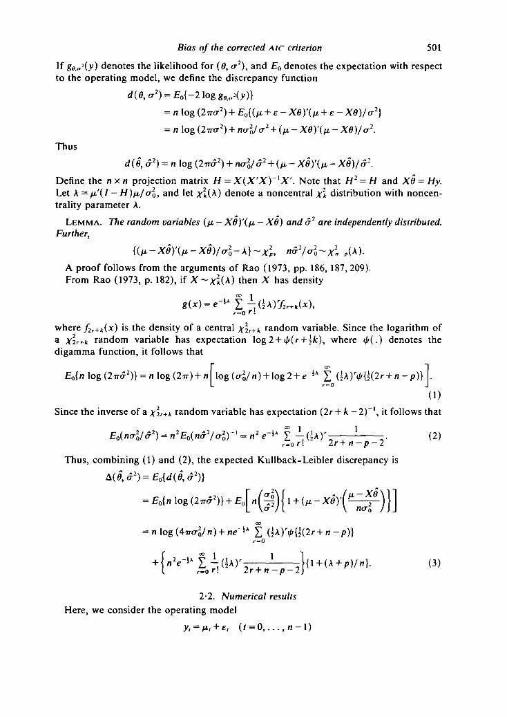
Fig. 1. Expected A I C C , shown by lines, A*, triangles, and AlC, circles, versus p. Trigonometric regression candidates,linear and exponential operating models; n = 100.

Bias of the corrected AIC criterion 503

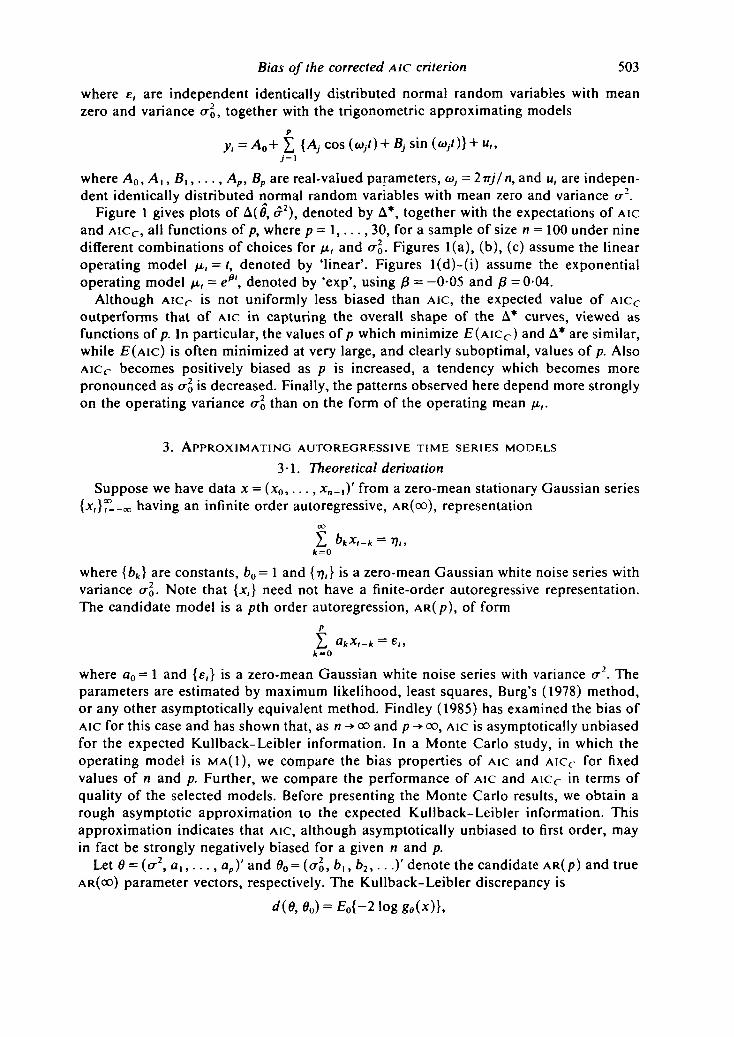
where e, are independent identically distributed normal random variables with meanzero and variance crl, together with the trigonometric approximating models

y, = A>+ I {Aj cos (tojt) + Bj sin («,-/)} + u,,

where Ao, At, B , , . . . , Ap, Bp are real-valued parameters, Wj = 2vj/n, and u, are indepen-dent identically distributed normal random variables with mean zero and variance a2.

Figure 1 gives plots of A(0, a2), denoted by A*, together with the expectations of AICand A IC C , all functions of p, where p = 1 , . . . , 30, for a sample of size n = 100 under ninedifferent combinations of choices for ft, and crl. Figures l(a), (b), (c) assume the linearoperating model fi, = t, denoted by 'linear'. Figures l(d)-(i) assume the exponentialoperating model /A, = ep', denoted by 'exp', using B = -0-05 and B = 004.

Although A I C C is not uniformly less biased than AIC, the expected value of AIC C

outperforms that of AIC in capturing the overall shape of the A* curves, viewed asfunctions of p. In particular, the values of p which minimize £ ( A I C C ) and A* are similar,while E ( A I C ) is often minimized at very large, and clearly suboptimal, values of p. AlsoA I C C becomes positively biased as p is increased, a tendency which becomes morepronounced as crl is decreased. Finally, the patterns observed here depend more stronglyon the operating variance al than on the form of the operating mean /A,.

3. APPROXIMATING AUTOREGRESSIVE TIME SERIES MODELS

3 • 1. Theoretical derivation

Suppose we have data x = ( x 0 , . . . . *„_,)' from a zero-mean stationary Gaussian series{x,}^._co having an infinite order autoregressive, AR(OO), representation

where {bk} are constants, bo= 1 and {17,} is a zero-mean Gaussian white noise series withvariance a\. Note that {x,} need not have a finite-order autoregressive representation.The candidate model is a pth order autoregression, AR(/>), of form

k-0

r2where ao= 1 and {e,} is a zero-mean Gaussian white noise series with variance cr2. Theparameters are estimated by maximum likelihood, least squares, Burg's (1978) method,or any other asymptotically equivalent method. Findley (1985) has examined the bias ofAIC for this case and has shown that, as n -» 00 and p -> 00, AIC is asymptotically unbiasedfor the expected Kullback-Leibler information. In a Monte Carlo study, in which theoperating model is MA(1) , we compare the bias properties of AIC and Aic r for fixedvalues of n and p. Further, we compare the performance of AIC and AIC C in terms ofquality of the selected models. Before presenting the Monte Carlo results, we obtain arough asymptotic approximation to the expected Kullback-Leibler information. Thisapproximation indicates that AIC, although asymptotically unbiased to first order, mayin fact be strongly negatively biased for a given n and p.

Let 6 = (a2, a , , . . . , ap) 'and 90={crl, 6,, b2,...)'denote the candidate AR(/>) and trueAR(OO) parameter vectors, respectively. The Kullback-Leibler discrepancy is

e,eo) = E0{-2\ogge(x)},

504 CLIFFORD M. HURVICH AND CHIH-LING TSAI

where ge(x) is the likelihood function for the candidate model parameters, and Eo denotesexpectation under the true model. Let 2fl and 1^ denote the n x n covariance matricesof x under the models with 6 and 0o, respectively. Since

- 2 log ge(x) = n log (27r) A

one obtains

d(6, d0) = n log (2TT) + log |2fl

Let 6 = (a2, a,,..., dp)' denote the estimated parameters in the candidate model. Notethat 0 need not be the maximum likelihood estimator. The selection methods AIC andA I C C may be viewed as estimators of the expected Kullback-Leibler information,

A(0) = E0{d{§, e0)} = n log (2TT)+ E0(log |2«|) + £0{tr (1^6% (4)

Denote the true spectral density by f(<o) for o» e [-IT, IT], and denote the AR(/>) spectralestimate by

where the sum is over the range k = 1 , . . . , p. From Parzen (1983, p. 235), the eigenvectorsand corresponding eigenvalues of S e may be approximated by

n-i{exp(-ia>,r)} (t = 0, ...,n- 1), 2irf(o}) (j = 0 , . . . , n - 1).

It follows that the expected Kullback-Leibler information A(0) may be approximated by

•rJ — TT

8(6) = E0{n log (2TTC72)} +W(27r )}£ 0 { / («) / /„(«)} dw.J —n

To obtain an approximation for the second term we use the result of Berk (1974). Ifp-KX>, n-too with p3/n->0 then fp(w) is asymptotically equivalent to the truncatedperiodogram estimator

f*(to) = — X crexp(iroj),2iT\r\<p

where1 n-\r\

Cr~~ L XlXl-\r\n i-o

is the sample autocovariance. From Bloomfield (1976, p. 191), we obtain the approxima-tions

From Bloomfield (1976, p. 196), if we define v = n/p, then the distribution of vf*(a>)/f(w)may be approximated by xl- If we treat all the above approximations as exact and assumethat fp((o) =f*(co) then we obtain

v-2 \-2pln

Thus

1 -2p/n(5)

Bias of the corrected AIC criterion 505

Note that, to first order, the approximation (5) to the expected Kullback-Leibler informa-tion has penalty term 2p/n, in agreement with that of AIC. Nevertheless, the full penaltyterm in (5) is (1 -2p/ n)~\ which is always larger, and potentially much larger, than thepenalty term of AIC, 2p/n. Thus, AIC may be strongly negatively biased. The Monte Carloresults given below, which do not rely on the approximations used in the above derivation,indicate that the exact penalty term of the expected Kullback-Leibler information is infact quite close to the penalty term of AICC, that is,

and that AICC is much less biased than AIC.

3-2. Monte Carlo resultsHere we present Monte Carlo results on the performance of AIC and AICC for

autoregressive time series model selection, when the operating model is Gaussian AR(OO).We study the finite-sample bias properties of AIC and AICC) viewed as estimators of A(0).We also study the quality of the models selected by AIC and AICC. The true model usedthroughout is the first-order moving average process x, = e, + 0-99e,_,, where {e,} areindependent and identically distributed standard normal. Note that {x,} has an AR(OO)representation, and cannot be written as a finite-order AR. For each of the sample sizesn = 23, 30, 40, 50, 75 and 100, we generated 100 independent realizations x 0 , . . . , xn_,of the moving average process. For each realization, autoregressive models of ordersp = I,... ,20 were fitted by the Burg method, and the criteria AIC, AICC and sic(Schwarz, 1978) were computed. The sic criterion is given by

sic = n log (2TT(T2) + p log n.

Also computed was d(6p, 0O), where the subscript in 0P has been added for clarity toexplicitly indicate model order. Averages of the criterion functions as well as d(0p, 0O)were computed over the 100 realizations. All these are functions of the candidate modelorder p. We denote the average of the 100 values of d(6p, 0O) by A(/>), or simply A. Notethat A serves as an approximation to the expected Kullback-Leibler information A(0r)defined in (4). Figure 2 shows that, almost without exception, AICC exhibits less biasthan AIC in estimating A. Furthermore, the magnitude of the bias of AIC increases withmodel order, while AICC remains nearly unbiased for all model orders. These resultsparallel those found for the overfitting case in Hurvich & Tsai (1989).

Next, we explore the quality of the models selected by AIC, AICC and sic. Since thereis no true finite autoregressive model order in the current study, we will measure qualityhere using the expected Kullback-Leibler discrepancy, instead of simply examining theselected model orders. Another reasonable measure of quality, prediction error, will beconsidered at the end of this section. For each realization, the criteria yielded selectedmodel orders P(AIC), /J(AICC), p(sic), and corresponding expected Kullback-Leiblerdiscrepancies AA,C = A{/5(AIC)}, AA]CV = A{p(Aicr)}, AS|C = A{/5(sic)}. In order to allowthese discrepancy values to be viewed relative to an absolute zero, the constant d(60, 0O)was subtracted, yielding

The average values of DAIC, DMCc and DSIC over the 100 realizations are given in Table1. For all sample sizes studied the average value of DAICr is less than those of DMC and

(a) n = 23 (b) n =

1200

»aa>«««666f luoooo o o o p

(c) n=40

20

or•n•n

0

0

C

120(d) n =

120(e) n = (f) n = 100

100

90

140 '

120 (-

115

I

zonEEi

ri

Fig. 2. Average AICC , shown by lines, A, triangles, and AIC, circles, versus candidate autoregressive model order, basedon 100 realizations of MA(1).

Bias of the corrected AIC criterion 507

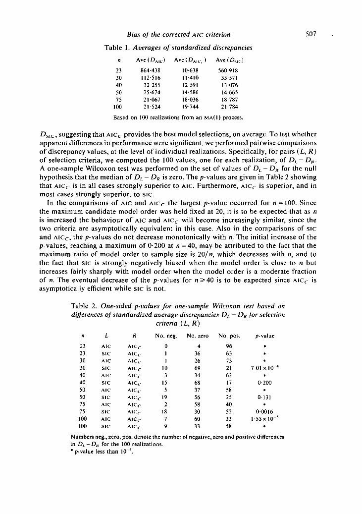
Table 1. Averages of standardized discrepancies

n Avc(DAIC) Ave(DA I C () Ave(D s l c)

2330405075

100

864-438112-51632-25525-6742106721-524

10-63811-41012-59114-5861803619-744

560-91833-5711307614-66518-78721-784

Based on 100 realizations from an M A ( 1 ) process.

DS\c, suggesting that AICC provides the best model selections, on average. To test whetherapparent differences in performance were significant, we performed pairwise comparisonsof discrepancy values, at the level of individual realizations. Specifically, for pairs (L, R)of selection criteria, we computed the 100 values, one for each realization, of DL-DR.A one-sample Wilcoxon test was performed on the set of values of DL - DR for the nullhypothesis that the median of DL — DR is zero. The p-values are given in Table 2 showingthat Aicr is in all cases strongly superior to AIC. Furthermore, AICC is superior, and inmost cases strongly superior, to sic.

In the comparisons of AIC and AICC the largest p-value occurred for n = 100. Sincethe maximum candidate model order was held fixed at 20, it is to be expected that as nis increased the behaviour of AIC and AICC will become increasingly similar, since thetwo criteria are asymptotically equivalent in this case. Also in the comparisons of sicand AICC, the p- values do not decrease monotonically with n. The initial increase of thep-values, reaching a maximum of 0-200 at n =40, may be attributed to the fact that themaximum ratio of model order to sample size is 20/ n, which decreases with n, and tothe fact that sic is strongly negatively biased when the model order is close to n butincreases fairly sharply with model order when the model order is a moderate fractionof n. The eventual decrease of the p-values for ns=40 is to be expected since AICC isasymptotically efficient while sic is not.

Table 2. One-sided p-values for one-sample Wilcoxon test based ondifferences of standardized average discrepancies DL — DRfor selection

criteria (L, R)

No. pos. p-valuen

23233030404050507575100100

L

AIC

SIC

AIC

SIC

AIC

SIC

AIC

SIC

AIC

SIC

AIC

SIC

R

AICC

AICC-A IC r

AICC

A I C r

A1CC

AIC (

AICC

A l C r

AIC r

A I C r

A I C r

No. neg.

011

103

155

192

1879

No. z

43626693468375658306033

966373216317582540523358

***

701 xlO*

0-200*

0131•

0-00161-55x10

*

Numbers neg., zero, pos. denote the number of negative, zero and positive differencesin DL- DR for the 100 realizations.* p-value less than 10~5.

508 CLIFFORD M. HURVICH AND CHIH-LING TSAI

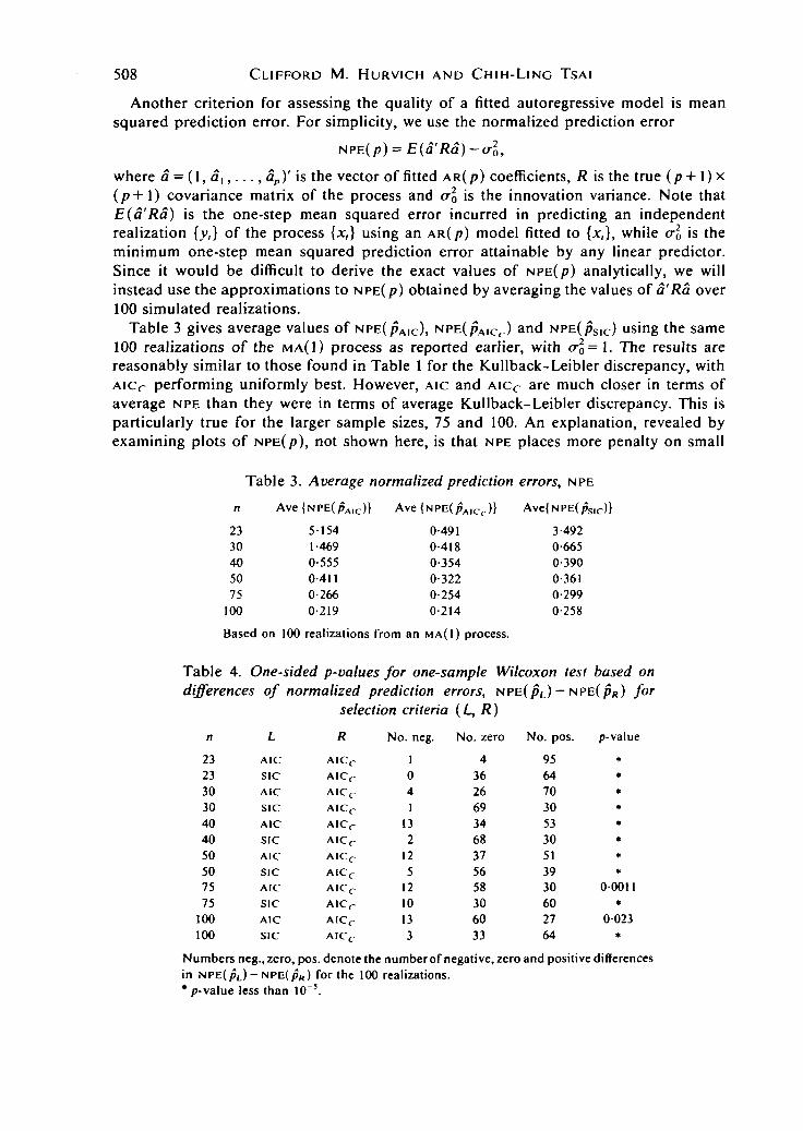
Another criterion for assessing the quality of a fitted autoregressive model is meansquared prediction error. For simplicity, we use the normalized prediction error

NPE( p) = E(a'Ra)-a20,

where a = (1, a , , . . . , ap)' is the vector of fitted AR(/>) coefficients, R is the true (p + l ) x(p + l) covariance matrix of the process and a\ is the innovation variance. Note thatE(d'Ra) is the one-step mean squared error incurred in predicting an independentrealization {>>,} of the process {x,} using an AR(/?) model fitted to {x,}, while <J\ is theminimum one-step mean squared prediction error attainable by any linear predictor.Since it would be difficult to derive the exact values of N P E ( P ) analytically, we willinstead use the approximations to NPE(/?) obtained by averaging the values of a'Ra over100 simulated realizations.

Table 3 gives average values of NPE(/5 A | C ) , NPE(/5A|Cf.) and NPE(/5S ) C) using the same100 realizations of the MA(1) process as reported earlier, with cr2

0= 1. The results arereasonably similar to those found in Table 1 for the Kullback-Leibler discrepancy, withAIC C performing uniformly best. However, AIC and AIC C are much closer in terms ofaverage NPE than they were in terms of average Kullback-Leibler discrepancy. This isparticularly true for the larger sample sizes, 75 and 100. An explanation, revealed byexamining plots of NPE(/>), not shown here, is that NPE places more penalty on small

Table 3. Average normalized prediction errors, NPE

n Ave{NPE(pAIC)} Ave{NPE(pAIC(.)} Ave{NPE(ps,c)}

2330405075

100

5-1541-4690-5550-4110-2660-219

0-4910-4180-3540-3220-2540-214

3-4920-6650-3900-3610-2990-258

Based on 100 realizations from an M A ( 1 ) process.

Table 4. One-sided p-values for one-sample Wilcoxon test based ondifferences of normalized prediction errors, N P E ( / 5 L ) - N P E ( P « ) for

selection criteria (L, R)

n

23233030404050507575

100100

L

AIC

SIC

AIC

SIC

AIC

SIC

AIC

SIC

AIC

SIC

AIC

SIC

R

AICC

AICC

AICC

AICC

AICC

AIC r

A I C r

A1CC

AICC

A I C r

AICC

A I C r

No. neg.

1041

132

125

1210133

No. zero

43626693468375658306033

No. pos.

956470305330513930602764

p-valu

*

**

***

0-001*

0023*

Numbers neg., zero, pos. denote the number of negative, zero and positive differencesin NPE(pJ-NPE(pR) for the 100 realizations.*p-value less than 10~5.

Bias of the corrected AIC criterion 509

model orders, and much less penalty on large model orders, than does the Kullback-Leibler discrepancy A.

Table 4 gives p- values for Wilcoxon tests on differences of the form NPE(/5L) - NPE(/JR)for pairs (L, R) of selection criteria; AICC is strongly superior to both AIC and sic interms of normalized prediction error for all cases studied. Compared with the case ofthe Kullback-Leibler criterion, Table 2, the superiority of AICC over AIC is somewhatweaker here for n = 75 and n = 100, while the superiority of AICC over sic is strongerhere than before. Both phenomena can be explained as above, since AIC tends to overfitand sic to underfit, compared with AICC-

ACKNOWLEDGEMENT

The authors are grateful to the referee for suggesting the consideration of predictionerror in the simulation study.

REFERENCES

AKAIKE, H. (1973). Information theory and an extension of the maximum likelihood principle. In 2ndInternational Symposium on Information Theory, Ed. B. N. Petrov and F. Csaki, pp. 267-81. Budapest:Akademia Kiado.

BERK, K.. (1974). Consistent autoregressive spectral estimates. Ann. Statist. 2, 489-502.BLOOMFIELD, P. (1976). Fourier Analysis of Time Series: An Introduction. New York: Wiley.BURG, J. P. (1978). A new analysis technique for time series data. In Modern Spectrum Analysis, ed. D. G.

Childers, pp. 42-8, New York: IEEE Press.FINDLEY, D. (1985). On the unbiasedness property of AIC for exact or approximating linear stochastic time

series models. J. Time Ser. Anal. 6, 229-52.HURVICH, C. M. & TSAI, C. L. (1989). Regression and time series model selection in small samples.

Biometrika 76, 297-307.LINHART, H. & ZUCCHINI, W. (1986). Model Selection. New York: Wiley.PARZEN, E. (1978). Some recent advances in time series modeling. In Modern Spectrum Analysis, Ed. D. G.

Childers, pp. 226-33. New York: IEEE Press.PARZEN, E. (1983). Autoregressive spectral estimation. In Handbook of Statistics, 3, Ed. D. R. Brillinger

and P. R. Krishnaiah, pp. 221-47. New York: Elsevier.RAO, C. R. (1973). Linear Statistical Inference and its Applications, 2nd ed. New York: Wiley.SCHWARZ, G. (1978). Estimating the dimension of a model. Ann. Statist. 6, 461-4.SHIBATA, R. (1980). Asymptotically efficient selection of the order of the model for estimating parameters

of a linear process. Ann. Statist. 8, 147-64.SHIBATA, R. (1981). An optimal selection of regression variables. Biometrika 68, 45-54.SUGIURA, N. (1978). Further analysis of the data by Akaike's information criterion and the finite corrections.

Comm. Statist. A 7, 13-26.

[Received June 1990. Revised November 1990]