Bi-objective mixed integer linear programming for managing buildingclusters with a shared electrical energy storage

Rui Dai, Hadi Charkhgard∗

Department of Industrial and Management System Engineering, University of South Florida, Tampa, FL, 33620USA

Abstract

Emerging smart grid infrastructures are allowing buildings to connect to components in other build-ings and utilize them in different ways. Clearly, these interconnected building clusters provide newopportunities for building operators to collaborate and help reduce their operational costs overa planning horizon. Nevertheless, since each building can be treated as an independent decisionmaker here, related fairness concerns have to be addressed in these collaborative environments. Weaddress these issues on building clusters when a single electrical energy storage is shared betweentwo buildings with deterministic demand. We introduce three energy storage sharing strategies,and develop a bi-objective mathematical formulation for each strategy. Several techniques suchas piecewise McCormick relaxation are employed for linearizing non-linear terms in the proposedformulations. An extensive computational study demonstrates the efficacy of our proposed lin-earization techniques, and compares all three strategies in terms of fairness and freedom.

Keywords: smart buildings, shared energy storage, piecewise McCormick relaxation, bi-objectivemixed integer linear programming

1. Introduction

Commercial and residential buildings are estimated to account for approximately 40% of theenergy consumption in the United States, see Table 1 (http://www.eia.gov/consumption). Hencethese infrastructures present significant potential for energy and cost savings. Two common ap-proaches for improving engery efficiency in buildings are to use (electrical and/or thermal) energystorage or on-site energy generation. These strategies are also shown in Figure 1. However, thesuccess of these approaches clearly depends upon applying optimal operational strategies, i.e., con-trolling/managing the entire system efficiently over a given planning horizon. Therefore it is notsurprising that the past two decades have seen numerous studies on developing such operationalregimes under different settings, i.e., constructed by ignoring/removing some components and/orarcs in Figure 1. Interested readers are referred to Bianchi et al. (2013); Liu and Henze (2006a,b);Lee et al. (2009); Bischi et al. (2014) for further details. Note that some studies have also as-sumed that building energy demands (Figure 1) are themselves uncertain and investigated furtherstrategies to deal with such conditions (Hu and Cho, 2014; Li et al., 2010).

∗Corresponding authorEmail address: hcharkhgard@usf.edu (Hadi Charkhgard )

Preprint submitted to – February 10, 2017

Table 1: Energy consumption estimates by sector

January to November 2016 2015 2014 2013 2012

Residential 21% 22% 22% 22% 21%

Commercial 18% 18% 19% 18% 18%

Industrial 31% 32% 32% 32% 32%

Transportation 29% 28% 27% 27% 28%

Power Grid

Electrical Energy Storage

Sell Buy

On-site Energy Generation Unit

Sell

Fuel

Thermal Energy Storage Heating and Cooling Systems

Buy

Building

Buy

Figure 1: Energy flow for single building using energy storage and on-site energy generation unit

Overall, most relevant studies have focused on developing optimal operational strategies for asingle building. Namely, the main assumption is that different buildings do not have any connection,and this assumption is quite reasonable in the context of traditional grids. However, newer smartgrid infrastructures (residential and commercial) are now allowing buildings to form “clusters” andshare energy by freely connecting with each other. In light of this, there is a critical need to developfurther optimal operational strategies for building clusters. Indeed, this topic has received very littleattention to date, with only a few known studies in this scope, i.e., AlSkaif et al. (2015); Dai et al.(2015); Hu et al. (2012, 2014).

Consequently, the goal of our research is to develop optimal operational strategies for buildingclusters in a smart grid. Hence consider an expanded view of Figure 1 with a cluster of multiplebuildings and their associated components, i.e., electrical and thermal energy storages, on-siteenergy generation units, and cooling and heating systems. In this generalized setting, each buildingcan freely connect to components in other buildings and utilize them in different ways. For example,at an arbitrary time, a building can decide to sell electrical energy stored in some storage to thepower grid to generate revenues. Alternatively, it may decide to charge up storages using one-sitegeneration units. However owing to high dimensionalities involved, solving the generalized multi-building problem imposes excessive complexity. Hence in this study, we focus on a specific case ofthis general problem, which is still highly-relevant to real-world operational settings.

It is well-known that energy storage can provide many benefits for building operators (Bathurstand Strbac, 2003; Chen et al., 2009; Sobieski and Bhavaraju, 1985; Walawalkar et al., 2007). Namely,these gains include 1) Backup Energy: buildings can use stored energy at times of power outagedue to disasters, cascading outages, and so on, 2) Energy Arbitrage Revenues: buildings can take

2

Power Grid

Electrical Energy Storage

Buy

Building 1

Buy

Building 2

Buy

Figure 2: Energy flow for building cluster with two buildings using a single electrical storage

advantage of dynamic pricing by purchasing and storing energy when the price is low (off-peaktimes) and re-selling it when the price is high (on-peak times), 3) Peak Shaving: Buildings can savecosts by storing energy when their demand is low (off-peak times) and using it when their demandis high (on-peak times). In light of this, the main contribution of our research is to develop noveltechniques for computing optimal operating strategies for the configuration shown in Figure 2, i.e.,when two buildings share a single electrical energy storage. We assume that the energy demand ofeach building is known for each time period in the entire planning horizon.

It is evident that each building can be treated as an independent decision maker that wants tooptimize its objective function, which is assumed to be its total operational cost. Hence given thatthere are two buildings, there is clear need for expanded bi-objective optimization here.

We note that in general sharing (electrical) energy storage facilities between buildings introducestwo further considerations, i.e., fairness and freedom. Now the term “fairness” is difficult to define,but one can reasonably assume that it means that the amount of energy a building charges intoan energy storage should be equal to the amount of energy that it discharges (uses). Similarly,the term “freedom” refers to how freely a building can discharge energy from an energy storage.Now obviously these two aims are conflicting and hence one can pursue a trade-off here. Forexample, increased freedom may save more costs for buildings, but at the same time may result ina completely unfair system (potentially leading to a breakdown of collaboration agreements betweenbuildings). Hence implementing trade-offs between fairness and freedom here is not obvious.

We develop three energy storage sharing strategies including extreme free strategy, extremefair strategy, and contract balance strategy. We present a novel bi-objective mixed integer linearprogramming formulation for the configuration shown in Figure 2 under each of these energy storagesharing strategies. It is worth mentioning that the contract balance strategy simply penalizes abuilding if it discharges more energy from the storage than what it actually charged into the storage(in entire planning horizon). The penalty is basically the cost that it has to be paid to the otherbuilding. To best of our knowledge, there is no study that has explored the consequences of thecontract balance strategy in this context. We develop a novel technique to measure the degree offairness and freedom of our proposed contract balance strategy. By conducting a comprehensivecomputational study, we show that the contract balance strategy is not only significantly betterthan the extreme free strategy in terms of fairness, but also it is significantly better than extremefair strategy in terms of cost savings.

It is worth mentioning that the proposed contract balance strategy yields bi-linear terms inthe mathematical formulation. As a result, properly handling these nonlinear terms and efficiently

3

linearizing them is a key challenge in itself. So, another contribution of our research is showinghow piecewise McCormick relaxation can be efficiently used for linearizing bi-linear terms with highlevel of precision.

The remainder of the paper is organized as follows. In Section 2, we introduce notation andsome fundamental concepts of multi-objective mixed integer linear programming. In Section 3, wepresent a basic bi-objective mixed integer linear programming formulation for computing optimaloperational strategies. In Section 4, we introduce three different energy storage sharing strategiesand show how the basic formulation can be customized for each of these strategies. In Section 5,we introduce a few techniques for linearizing the bi-objective formulation of the proposed contractbalance strategy. In Section 6, we conduct a computational study. Finally, in Section 7, we givesome concluding remarks.

2. Preliminaries

In this section, we introduce some necessary notations and concepts related to multi-objectivemixed integer linear programs (MOMILPs) to facilitate presentation and discussion of other sections.Foremost, a MOMILP can be stated as follows:

min(x,y)∈F

{z1(x, y), . . . , zp(x, y)}, (1)

where F :={

(x, y) ∈ Zn1+ ×Rn2

+ : Ax+ Ay ≤ b}

represents the feasible set in the decision space, andzi(x, y) = cix + ciy for each i = 1, . . . , p represents a linear objective function.The image O of Funder vector-valued function z = {z1, . . . , zp} represents the feasible set in the objective/criterionspace, i.e., O := z(F) := {o ∈ Rp : o = z(x, y) for some (x, y) ∈ F}. It is assumed that F is bounded,and all coefficients/parameters are rational, i.e., A ∈ Qm×n1 , A ∈ Qm×n2 , and ci, ci ∈ Qn1+n2 forall i = 1, . . . , p. Note that the term multi-objective linear program (MOLP) is also used sometimesif n1 = 0, and the term multi-objective integer linear program (MOILP) if n2 = 0.

Definition 1. A feasible solution (x′, y′) ∈ F is called efficient or Pareto optimal, if there is noother (x, y) ∈ F such that zk(x, y) ≤ zk(x

′, y′) for k = 1, . . . , p and z(x, y) 6= z(x′, y′). If (x′, y′) isefficient, then z(x′, y′) is called a nondominated point. The set of all efficient solutions (x′, y′) ∈ Fis denoted by FE. The set of all nondominated points z(x′, y′) ∈ O for some (x′, y′) ∈ FE is denotedby ON and referred to as the nondominated frontier or the efficient frontier.

Definition 2. Let (x′, y′) ∈ FE. If there is a λ ∈ Rp> such that (x′, y′) is an optimal solutionto min(x,y)∈F λ

T z(x, y), then (x′, y′) is called a supported efficient solution and z(x′, y′) is called asupported nondominated point.

Definition 3. Let Oe be the set of extreme points of the convex hull of O. A point z(x′, y′) ∈ O iscalled an extreme supported nondominated point if z(x′, y′) is a supported nondominated point andz(x′, y′) ∈ Oe.

Overall, multi-objective optimization is concerned with finding all nondominated points, i.e.,supported as well as unsupported nondominated points. Specifically, min(x,y)∈F z(x, y) is definedto be precisely ON . Now it is well-known that both the set of efficient solutions FE and theset of nondominated points ON of a MOLP are supported and connected, i.e., between any pair

4

(a) MOLP. (b) MOILP. (c) MOMILP.

Figure 3: An illustration of the nondominated frontier with only two objectives

of nondominated points there exists a sequence of nondominated points with the property thatall points on the line segment between consecutive points in the sequence are also nondominated(Isermann, 1977). Consequently, for a MOLP to describe all nondominated points, it suffices tofind all extreme supported nondominated points. An illustration of the nondominated frontier ofa MOLP when p = 2 is shown in Figure 3a, i.e., where the horizontal line shows the first objectivevalue and the vertical line shows the second objective value.

Now the set of nondominated points of a MOILP is finite (since by assumption F is bounded).However, unfortunately, due to the existence of unsupported nondominated points, finding allnondominated points of a MOILP is much more challenging. Along these lines, the nondominatedfrontier of a MOILP when p = 2 is also shown in Figure 3b where the red rectangles are unsupported.Finding all nondominated points of a MOMILP is even more challenging. Namely, if at most one ofthe objective functions contains continuous decision variables, then the set of nondominated pointsis finite and existing MOILP solution approaches can be applied to solve a MOMILP. However, inall other cases the efficient frontier of a MOMILP may contain connected parts as well as supportedand unsupported nondominated points. Therefore, in these cases, the set of nondominated pointsis not finite and existing algorithms for solving a MOILP cannot be used. An illustration of thenondominated frontier of a MOMILP when p = 2 is shown in Figure 3c as well, i.e., where evenhalf-open (or open) line segments may exist in the nondominated frontier. Interested readers arereferred to Belotti et al. (2013); Dachert (2014); Ehrgott (2006); Stidsen et al. (2014); Vincent et al.(2013) for further details on algorithms for MOILPs and MOMILPs.

zI

zN

Figure 4: Ideal point and nadir point of a MOMILP with p = 2

The following concepts are also helpful. A representation of these concepts is given in Figure 4.

5

(a) Iteration 0. (b) Iteration 1. (c) Iteration 2.

Figure 5: Progression of TSM in terms of the discovery of nondominated points

Definition 4. The point zI ∈ Rp is the ideal point if zIi = min(x,y)∈FE zi(x, y) for all i ∈ {1, . . . , p}.

Definition 5. The point zN ∈ Rp is the nadir point if zNi = max(x,y)∈FE zi(x, y) for all i ∈{1, . . . , p}.

It is also worth mentioning that the proposed formulations in this study are all bi-objectivemixed integer linear programs, i.e., MOMILPs with p = 2. There are a few algorithms that cansolve a bi-objective mixed integer linear program. In this study, we use the triangle slitting method(TSM), which is one of the most efficient algorithms (Boland et al., 2015). We next present ahigh-level description of the algorithm.

TSM works by first resolving the endpoints of the nondominated frontier. These two points arethen used to define a rectangle containing all the “not yet found” nondominated points, as shownin Figure 5a. The algorithm then tries to find the locally extreme supported nondominated pointswithin the rectangle. Now it can be shown that by finding these points, the rectangle can be splitinto a set of right-angled triangles containing all “not yet found” nondominated points, as shownfurther in Figure 5b. The algorithm then checks each of these triangles individually to find out ifthe hypotenuse of each is part of the nondominated frontier. If that is the case, then the triangleis removed from the list, otherwise it is split into at most two other rectangles. This operation isfurther illustrated in Figure 5c, where the hypotenuse of the top triangle in Figure 5b is not partof the nondominated frontier so it is split into two new rectangles. The algorithm repeats theseprocedures until finding a full representation of the nondominated frontier.

3. A basic bi-objective mixed integer linear programming formulation

In this section, we develop a basic bi-objective mixed integer linear programming formulationfor computing optimal operational strategies in building clusters when a single electrical energystorage is shared between two buildings with deterministic demand (see Figure 2). For simplicity,we assume that the electricity flow is at steady state, and cables are incapable of losing energy.However, we assume that some amount of energy may be lost while charging and discharging theelectrical energy storage. Furthermore, we assume that the electrical energy storage cannot be atcharging and discharging states at the same time. The main parameters and decision variablesused in the basic formulation are given Tables 2 and 3.

6

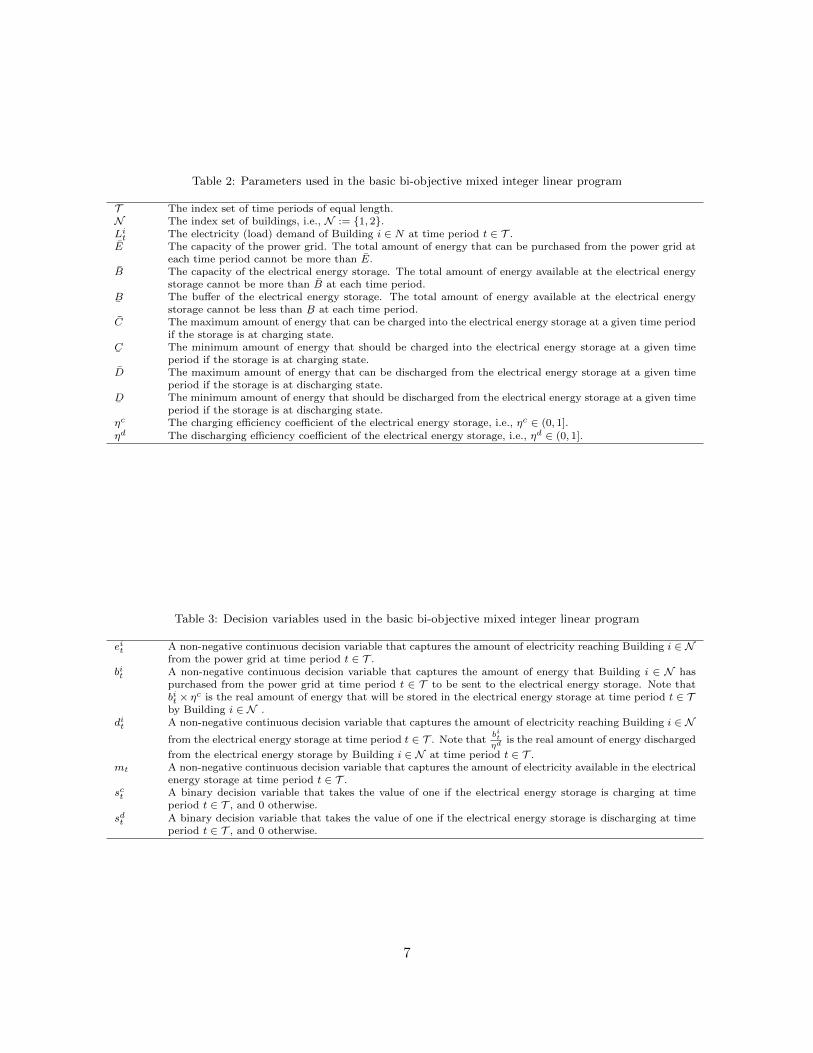
Table 2: Parameters used in the basic bi-objective mixed integer linear program

T The index set of time periods of equal length.N The index set of buildings, i.e., N := {1, 2}.Lit The electricity (load) demand of Building i ∈ N at time period t ∈ T .E The capacity of the prower grid. The total amount of energy that can be purchased from the power grid at

each time period cannot be more than E.B The capacity of the electrical energy storage. The total amount of energy available at the electrical energy

storage cannot be more than B at each time period.

¯B The buffer of the electrical energy storage. The total amount of energy available at the electrical energy

storage cannot be less than¯B at each time period.

C The maximum amount of energy that can be charged into the electrical energy storage at a given time periodif the storage is at charging state.

¯C The minimum amount of energy that should be charged into the electrical energy storage at a given time

period if the storage is at charging state.D The maximum amount of energy that can be discharged from the electrical energy storage at a given time

period if the storage is at discharging state.

¯D The minimum amount of energy that should be discharged from the electrical energy storage at a given time

period if the storage is at discharging state.ηc The charging efficiency coefficient of the electrical energy storage, i.e., ηc ∈ (0, 1].ηd The discharging efficiency coefficient of the electrical energy storage, i.e., ηd ∈ (0, 1].

Table 3: Decision variables used in the basic bi-objective mixed integer linear program

eit A non-negative continuous decision variable that captures the amount of electricity reaching Building i ∈ Nfrom the power grid at time period t ∈ T .

bit A non-negative continuous decision variable that captures the amount of energy that Building i ∈ N haspurchased from the power grid at time period t ∈ T to be sent to the electrical energy storage. Note thatbit × ηc is the real amount of energy that will be stored in the electrical energy storage at time period t ∈ Tby Building i ∈ N .

dit A non-negative continuous decision variable that captures the amount of electricity reaching Building i ∈ Nfrom the electrical energy storage at time period t ∈ T . Note that

bitηd

is the real amount of energy discharged

from the electrical energy storage by Building i ∈ N at time period t ∈ T .mt A non-negative continuous decision variable that captures the amount of electricity available in the electrical

energy storage at time period t ∈ T .sct A binary decision variable that takes the value of one if the electrical energy storage is charging at time

period t ∈ T , and 0 otherwise.sdt A binary decision variable that takes the value of one if the electrical energy storage is discharging at time

period t ∈ T , and 0 otherwise.

7

The basic bi-objective mixed integer linear programming formulation can be written as,

min {z1, z2} (2)

s.t.∑i∈N

(eit + bit) ≤ E ∀t ∈ T (3)

eit + dit = Lit ∀i ∈ N ,∀t ∈ T , (4)

sct + sdt ≤ 1 ∀t ∈ T , (5)

¯Csct ≤

∑i∈N

bitηc ≤ Csct ∀t ∈ T , (6)

¯Dsdt ≤

∑i∈N

ditηd≤ Dsdt ∀t ∈ T , (7)

∑i∈N

bitηc −

∑i∈N

ditηd

= mt −mt−1 ∀t ∈ T , (8)

¯B ≤ mt ≤ B ∀t ∈ T , (9)

eit, bit, d

it,mt ≥ 0 i ∈ N , t ∈ T (10)

sct , sdt ∈ {0, 1} t ∈ T (11)

where z1 is the objective function of the first building and z2 is the objective function of the secondbuilding. We will discuss about these functions in Section 4. Constraints (3) ensure that theamount of electricity purchased from the power gird is restricted by the capacity of the power gridat each time period. Constraints (4) guarantee that the total amount of electricity purchased fromthe power grid and also discharged from the electrical energy storage will cover the total electricityload of each building at each time period. Constraints (5) ensure that the state of the electricalenergy storage cannot be charging and discharging at the same time. Constraints (6) and (7)ensure that the amount of energy charged and/or discharged from the electrical energy storage iswithin the allowed range at any time period. Constraints (8) impose the energy conservation inthe electrical energy storage at any time period. Finally, Constraints (9) ensure that the amountof energy available at the electrical energy storage is within the allowed range at any time period.Note that, for simplicity, we assume that

m0 = m|T | = ¯B. (12)

So, this should also be added to the formulation.

4. The trade-off between fairness and freedom

As it is mentioned in Introduction, we assume that each building is an independent decisionmaker that wants to minimize its own total cost. However, the shared electrical energy storageintroduces two further considerations, i.e., fairness and freedom. Three different energy storagesharing strategies are introduced in this section to deal with the trade-off between fairness andfreedom. We show how the basic formulation presented in Section 3 can be customized for each ofthese strategies.

8

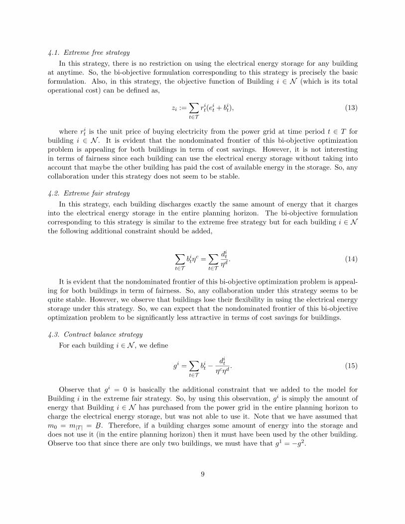
4.1. Extreme free strategy

In this strategy, there is no restriction on using the electrical energy storage for any buildingat anytime. So, the bi-objective formulation corresponding to this strategy is precisely the basicformulation. Also, in this strategy, the objective function of Building i ∈ N (which is its totaloperational cost) can be defined as,

zi :=∑t∈T

rit(eit + bit), (13)

where rit is the unit price of buying electricity from the power grid at time period t ∈ T forbuilding i ∈ N . It is evident that the nondominated frontier of this bi-objective optimizationproblem is appealing for both buildings in term of cost savings. However, it is not interestingin terms of fairness since each building can use the electrical energy storage without taking intoaccount that maybe the other building has paid the cost of available energy in the storage. So, anycollaboration under this strategy does not seem to be stable.

4.2. Extreme fair strategy

In this strategy, each building discharges exactly the same amount of energy that it chargesinto the electrical energy storage in the entire planning horizon. The bi-objective formulationcorresponding to this strategy is similar to the extreme free strategy but for each building i ∈ Nthe following additional constraint should be added,

∑t∈T

bitηc =

∑t∈T

ditηd. (14)

It is evident that the nondominated frontier of this bi-objective optimization problem is appeal-ing for both buildings in term of fairness. So, any collaboration under this strategy seems to bequite stable. However, we observe that buildings lose their flexibility in using the electrical energystorage under this strategy. So, we can expect that the nondominated frontier of this bi-objectiveoptimization problem to be significantly less attractive in terms of cost savings for buildings.

4.3. Contract balance strategy

For each building i ∈ N , we define

gi =∑t∈T

bit −ditηcηd

. (15)

Observe that gi = 0 is basically the additional constraint that we added to the model forBuilding i in the extreme fair strategy. So, by using this observation, gi is simply the amount ofenergy that Building i ∈ N has purchased from the power grid in the entire planning horizon tocharge the electrical energy storage, but was not able to use it. Note that we have assumed thatm0 = m|T | =

¯B. Therefore, if a building charges some amount of energy into the storage and

does not use it (in the entire planning horizon) then it must have been used by the other building.Observe too that since there are only two buildings, we must have that g1 = −g2.

9

By using this definition, in this strategy, if gi > 0 for Building i ∈ N then the other buildingwill be penalized. The penalty is basically the cost that has to be paid to Building i by Buildingi′ ∈ N\{i}. We assume that the penalty is equal to rigi where∑

t∈Tritb

it = ri

∑t∈T

bit (16)

So, ri is basically the average unit price of electricity that Building i has purchased from thepower grid to charge the electrical energy storage in the entire planning horizon. So, rigi can beinterpreted as the refund to Building i for the amount of energy that it has purchased but wasnot able to use. Consequently, the bi-objective formulation of the contract balance strategy is asfollows,

min z1 :=∑t∈T

r1t (e

1t + b1t )−max{r1g1, 0}+ max{r2g2, 0} (17)

min z2 :=∑t∈T

r2t (e

2t + b2t )−max{r2g2, 0}+ max{r1g1, 0} (18)

s.t. (3)− (12), (15), (16)

g1, g2 ∈ R (19)

r1, r2 ≥ 0 (20)

Note that this formulation contains some nonlinear terms in the objective functions and Con-straints (16).

5. Linearizing the formulation of contract balance strategy

Note that to best of our knowledge, there is no exact solver for bi-objective mixed integernon-linear programs. Consequently, to be able to use the power of TSM, we next explain how thebi-objective formulation of the contract balance strategy can be efficiently linearized (with highlevel of precision).

5.1. Removing the max functions in the objective functions

In the objective functions, there are two max functions. Removing these functions can be doneeasily by introducing two new non-negative continuous variables, i.e., g1, g2, one binary variable,i.e., y ∈ {0, 1}, and a few additional constraints. So, objective functions (17) and (18) should bereplaced by

min z1 :=∑t∈T

r1t (e

1t + b1t )− r1g1 + r2g2 (21)

min z2 :=∑t∈T

r2t (e

2t + b2t )− r2g2 + r1g1 (22)

10

s.t. g1 ≤ g1 (23)

g1 ≤My (24)

g1 ≤ g1 +M(1− y) (25)

g2 ≤ g2 (26)

g2 ≤M(1− y) (27)

g2 ≤ g2 +My (28)

g1, g2 ≥ 0 (29)

y ∈ {0, 1}, (30)

where M is a sufficiently large value. The additional constraints ensure that g1 = max{0, g1} andg2 = max{0, g2}. Furthermore, we know that g1 = −g2. Hence, either g1 = 0 or g2 = 0 (or both).This observation is captured by introducing the new binary decision variable, i.e., y. Observe thatif y = 0 then g1 = 0 (and g2 = g2), and also if y = 1 then g2 = 0 (and g1 = g1).

5.2. Linearizing bi-linear terms

Although we were able to remove the max functions in both objective functions, there are stillmultiple bi-linear terms in both objective functions (21) and (22), and Constraints (16) includingrigi for each i ∈ N , and ribit for each i ∈ N and t ∈ T .

A widely used approach to linearize (continuous) bi-linear terms when a lower bound and anupper bound are known for each variable in the bi-linear term is McCormick relaxation (McCormick,1976). Suppose that we would like to linearize the bi-linear term x1x2 where we know that xL1 ≤x1 ≤ xU1 and xL2 ≤ x2 ≤ xU2 . In McCormick relaxation, any instance of x1x2 will be replaced by anew variable, denoted by w, and the following additional linear constraints (sometimes referred toas McCormick envelopes) should be added to the model,

w ≥ xL1 x2 + x1xL2 − xL1 xL2

w ≥ xU1 x2 + x1xU2 − xU1 xU2

w ≤ xU1 x2 + x1xL2 − xU1 xL2

w ≤ xL1 x2 + x1xU2 − xL1 xU2

w ∈ R.

To increase the accuracy of the standard McCormick relaxation, we can partition the domain ofthe variables to obtain a tighter relaxation. In this case, a new set of binary variables should beintroduced to make sure that only one of the generated search regions is active at any time. This isknown as piecewise McCormick relaxation (Castro, 2015). For example, by partitioning the domainof x1 into 3 pieces, and the domain of x2 into 4 pieces a total of 3× 4 = 12 search regions will beconstructed. Consequently, 12 sets of McCormick envelopes should be added to the formulation.Also, 12 new binary variables should be introduced, and we need to make sure that only one ofthese 12 search regions is active at anytime. So, we observe that piecewise McCormick relaxationcan exponentially increase the size of the formulation.

Figure 6 shows the co-occurrence graph for bi-linear terms in the (revised) formulation of thecontract balance strategy. In this graph nodes represent decision variables, and links represent theexistence of corresponding bi-linear terms in the formulation. We observe that in all bi-linear terms

11

b1|T |

r1g1

b11

b12

b2|T |

r2g2

b21

b22

Figure 6: Co-occurrence graph for bi-linear terms.

either r1 or r2 exist. That implies that to obtain tighter relaxations, we may only partition thedomain of these two variables. By considering this observation, we next linearize all bi-linear termsof the formulation by using piecewise McCormick relaxation.

We first note that:

• bit ∈ [ ¯Cηc ,

Cηc ] for all i ∈ N and t ∈ T .

• ri ∈ [¯R, R] for all i ∈ N where

¯R := min{rit : i ∈ N , t ∈ T } and R := max{rit : i ∈ N , t ∈ T }.

• gi ∈ [¯G, G] for all i ∈ N where

¯G := 0 and G :=

|T |max{ Cηc, Dηc}

2 . The latter, i.e., the upperbound, can be obtained by assuming that one building only charges the electrical energystorage and the other only discharges. So, given that the storage cannot be at the chargingand discharging states at the same time, the result follows.

We assume that the domain of r1 and r2, i.e., [¯R, R], has to be partitioned into K equal pieces.

Consequently, for each k = 1, . . . ,K, we define

¯Rik :=

¯Ri +

(Ri −¯Ri)(k − 1)

K∀i ∈ N

Rik :=¯Ri +

(Ri −¯Ri)k

K∀i ∈ N .

By using theses parameters, and applying piecewise McCormick relaxation, the bi-objectivemixed integer linear programming formulation of the proposed contract balance strategy is asfollows,

min z1 :=∑t∈T

r1t (e

1t + b1t )− v1 + v2 (31)

min z2 :=∑t∈T

r2t (e

2t + b2t )− v2 + v1 (32)

s.t. (3)− (12), (15), (19), (23)− (30)∑t∈T

ritbit =

∑t∈T

wit ∀i ∈ N (33)

12

gi =

K∑k=1

gik ∀i ∈ N (34)

bit =K∑k=1

bitk ∀i ∈ N ,∀t ∈ T (35)

K∑k=1

yik = 1 ∀i ∈ N (36)

yik¯Rik ≤ rik ≤ yikRik ∀i ∈ N ,∀k ∈ {1, . . . ,K} (37)

yik ¯G ≤ gik ≤ yikG ∀i ∈ N ,∀k ∈ {1, . . . ,K} (38)

yik ¯C

ηc≤ bitk ≤ yik

C

ηc∀i ∈ N ,∀t ∈ T ,∀k ∈ {1, . . . ,K} (39)

vi ≥K∑k=1

(¯Rikg

ik + rik ¯

G− yik¯Rik ¯G) ∀i ∈ N (40)

vi ≥K∑k=1

(Rikgik + rikG− yikRikG) ∀i ∈ N (41)

vi ≤K∑k=1

(Rikgik + rik ¯

G− yikRik ¯G) ∀i ∈ N (42)

vi ≤K∑k=1

(¯Rikg

ik + rikG− yik¯

RikG) ∀i ∈ N (43)

wit ≥K∑k=1

(¯Rikb

itk + rik ¯

C

ηc− yik¯

Rik ¯C

ηc) ∀i ∈ N ,∀t ∈ T (44)

wit ≥K∑k=1

(Rikbitk + rik

C

ηc− yikRik

C

ηc) ∀i ∈ N ,∀t ∈ T (45)

wit ≤K∑k=1

(Rikbitk + rik ¯

C

ηc− yikRik ¯

C

ηc) ∀i ∈ N ,∀t ∈ T (46)

wit ≤K∑k=1

(¯Rikb

itk + rik

C

ηc− yik¯

RikC

ηc) ∀i ∈ N ,∀t ∈ T (47)

vi, wit, gik, r

ik, b

itk ≥ 0 ∀i ∈ N ,∀t ∈ T ,∀k ∈ {1, . . . ,K} (48)

yik ∈ {0, 1} ∀i ∈ N ,∀k ∈ {1, . . . ,K}, (49)

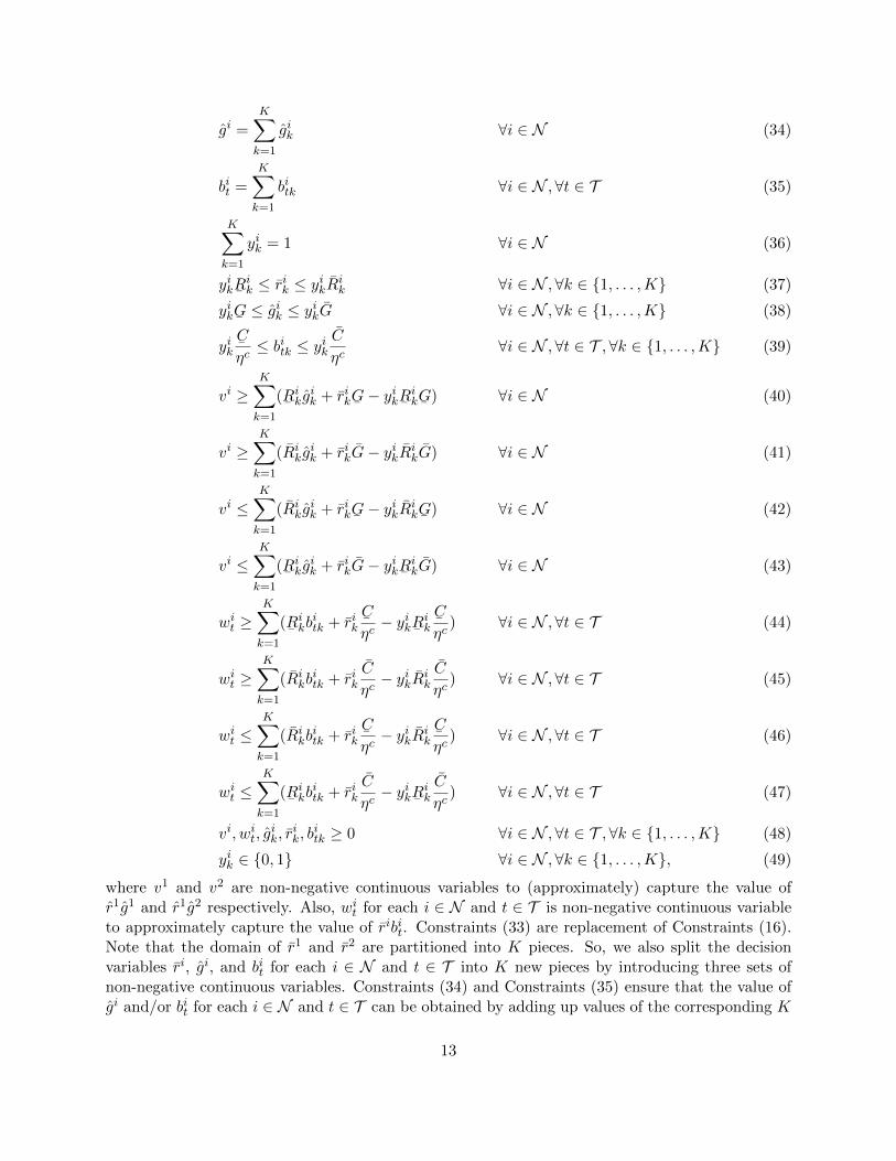
where v1 and v2 are non-negative continuous variables to (approximately) capture the value ofr1g1 and r1g2 respectively. Also, wit for each i ∈ N and t ∈ T is non-negative continuous variableto approximately capture the value of ribit. Constraints (33) are replacement of Constraints (16).Note that the domain of r1 and r2 are partitioned into K pieces. So, we also split the decisionvariables ri, gi, and bit for each i ∈ N and t ∈ T into K new pieces by introducing three sets ofnon-negative continuous variables. Constraints (34) and Constraints (35) ensure that the value ofgi and/or bit for each i ∈ N and t ∈ T can be obtained by adding up values of the corresponding K

13

new decision variables. Note that there is no need to add any constraint of the form ri =∑K

k=1 rik

since ri is not used in this formulation. Again since the domain of ri where t ∈ N is partitioned intoK pieces, we introduce K binary variables, denoted by yi1, . . . , y

iK , for activating/deactivating the

search regions/pieces. In particular, Constraints (36) to (39) ensure that exactly one piece is activeat anytime. They also guarantee that if yik = 1 for some i ∈ N and k ∈ {1, . . . ,K}, then we musthave that rik′ = gik′ = bitk′ = 0 for all k′ 6= k. Finally, Constraints (40) to (47) are simply McCormickenvelopes to capture the value of vi and wit for each i ∈ N and t ∈ T . Note that we know thatthe total operational cost of building i ∈ N cannot be smaller than

∑t∈T ¯

RLit. Consequently, toimprove the formulation, we suggest to add the following valid inequalities as well,∑

t∈Tr1t (e

1t + b1t )− v1 + v2 ≥

∑t∈T

¯RL1

t (50)∑t∈T

r2t (e

2t + b2t )− v2 + v1 ≥

∑t∈T

¯RL2

t . (51)

6. Computational Results

To evaluate the performance of the extreme free, extreme fair, and contract balance strategies,we conducted a comprehensive computational study. We used C++ to implement all formulations,and employed TSM to exactly solve each instance. In this computational study, TSM uses CPLEX12.7 as the single-objective integer programming solver. All computational experiments have beencarried out on a Dell PowerEdge R630 with two Intel Xeon E5-2650 2.2 GHz 12-Core Processors(30MB), 128GB RAM, and the RedHat Enterprise Linux 6.8 operating system, and using a singlethread.

We assumed that each time period represents one hour, and the entire planning horizon contains24 hours, i.e., |T | = 24. Based on this assumption, we generated 100 instances by randomly drawingrit and Lit for each i ∈ N and T ∈ T from a discrete uniform distribution on the interval [1, 20].Obviously, in this case, the demand load of each building at any time cannot be more than 20.So, since there are two buildings, we simply assume that B = 2 × 20 = 40, and

¯B = 1 for each

instance. Furthermore, we assume that C = D = 0.2× B and¯C =

¯D = 0.05× B. It is also worth

mentioning that the value of M can be safely set to G+ 1 (by definition).This computational study has three sections to achieve the following three goals:

• Demonstrating the performance of the proposed piecewise McCormick relaxation (for thecontract balance strategy) and choosing a proper value for the number of pieces, i.e., K.

• Comparing the extreme free, extreme fair strategy, and contract balance strategies in termsof fairness and freedom.

• Showing the performance of the proposed formulation for the contract balance strategy whenthe goal is to compute an approximate nondominated frontier.

6.1. Performance of the proposed piecewise McCormick relaxation

We first note that after computing any feasible solution for the proposed piecewise McCormickrelaxation, it is easy to compute the precise value of r1, r2. It is evident that if the value of rigi isclose to vi for each i ∈ N , then the quality of the (approximate) solution is good. So, by using this

14

0 10 20 30 40 50 60 70 80 90 1000

50

100

150

200

250

300

350

400

Instance

Qua

lity

Gap

(%

)

Piecewise Num: 1Piecewise Num: 2Piecewise Num: 4Piecewise Num: 8Piecewise Num: 16Piecewise Num: 32Piecewise Num: 64

Figure 7: Quality gap of each instance for different values of K

observation, for any feasible solution of the proposed piecewise McCormick relaxation, the followingformula measures its quality,

max{|100(rigi − vi)rigi + 0.001

| : i ∈ N}.

Note that we are only interested in efficient solutions, but there may be an infinite number ofefficient solutions corresponding to the proposed piecewise McCormick relaxation. So, we cannotcompute the proposed quality gap for all efficient solutions. So, instead, we compute the proposedgap for only two feasible solutions including:

• Solution 1: The optimal solution obtained by minimizing only the first objective functionin the proposed piecewise McCormick relaxation.

• Solution 2: The optimal solution obtained by minimizing only the second objective functionin the proposed piecewise McCormick relaxation.

In Figure 7, we have reported the worst quality gap obtained among these two solutions for allinstances and for different values of K. Observe that the proposed quality gap decreases dramati-cally by increasing the value of K. For example, the quality gap of Instance 30 is decreased fromaround 300% to 50% by increasing the value of K from 1 to only 16.

In Figure 8, the average quality gap of Solution 1 and its average computing time amongall instances for different values of K are given. Not surprisingly, the cost of computing betterapproximation is a dramatic increase in the solution time. We also observe that K = 32 seemsto have a reasonable balance between solution time and the quality gap. So, for most of ourexperiments we will set K = 32.

The nondominated frontier of the proposed piecewise McCormick relaxation for different valuesof K on one of the instances are shown in Figure 9. Not surprisingly, increasing the value of K

15

0 10 20 30 40 50 60 700

2

4

6

8

10

12

14

16

Piecewise Number

Ave

rage

Run

time

(s)

(a) Run time

0 10 20 30 40 50 60 700

20

40

60

80

100

120

140

160

180

Piecewise Number

Ave

rage

Qua

lity

Gap

(%

)

(b) Quality gap

Figure 8: Performance of piecewise McCormick relaxation for different values of K on average

2000 2200 2400 2600 2800 3000 3200 3400 36001400

1600

1800

2000

2200

2400

2600

2800

3000

Operational Cost of Building 1

Ope

ratio

nal C

ost o

f Bui

ldin

g 2

Piecewise Num: 1Piecewise Num: 2Piecewise Num: 4Piecewise Num: 8Piecewise Num: 16Piecewise Num: 32

Figure 9: The nondominated frontier for different values of K

16

is causing a shift in the nondominated frontier toward increasing both objective values, i.e., thefrontier is moved away from the origin. We also observe that the nondominated frontier has almostreached to its steady state for K = 32, i.e., not much has changed between K = 16 and K = 32.

6.2. Fairness vs freedom

In this section, we develop a technique to evaluate the freedom and fairness of an energy storagesharing strategy. We then demonstrate the effectiveness of the proposed contract balance strategyin contrast to the extreme free and fair strategies. We first make two observations:

Observation 6. The extreme free strategy can significantly benefit from the energy arbitrage. So,we expect that the end-points of the nondominated frontier in this strategy to be far away from eachother. This implies that the ideal point of the nondominated frontier corresponding to this strategyis expected to provide a lower bound for ideal points of other strategies. Similarly, its nadir pointis expected to provide an upper bound for nadir points of other strategies.

Observation 7. The extreme fair strategy is quite limiting and so (almost) cannot benefit fromthe energy arbitrage. So, we expect that the end-points of the nondominated frontier in this strategyto be quite close to each other. This implies that the ideal point of the nondominated frontier cor-responding to this strategy is expected to provide an upper bound for ideal points of other strategies.Similarly, its nadir point is expected to provide a lower bound for nadir points of other strategies.

2000 2500 3000 3500 4000

1500

2000

2500

3000

3500

Operational Cost of Building 1

Ope

ratio

nal C

ost o

f Bui

ldin

g 2

Extreme Free StrategyContract Balance StrategyExtreme Fair Strategy

Nadir Point ofFair Strategy

Nadir Point ofBalance Strategy

Ideal Point ofFree Strategy

Ideal Point ofBalance Strategy

Ideal Point ofFair Strategy

Nadir Point ofFree Strategy

Figure 10: Nondominated frontiers of different strategies

17

Figure 10 shows the nondominated frontier of all three strategies for one of the instances. Thecorrectness of Observations 6 and 7 can be clearly seen in this figure. So, by using these twoobservations, the degree of freedom of an energy storage sharing strategy can be defined as theEuclidean distance between the ideal point of its nondominated frontier and the ideal point ofthe nondominated frontier of the extreme free strategy. Note that smaller distances imply higherfreedom (i.e., more cost savings). Similarly, the degree of fairness of an energy storage sharingstrategy can be defined as the Euclidean distance between the nadir point of its nondominatedfrontier and the nadir point of the nondominated frontier of the extreme fair strategy. Note thatagain smaller distances imply higher fairness.

Let s1, s2, and s3 represent the extreme free, cost balance, and extreme fair strategies, respec-tively. Also, let I(s) and N(s) be the degree of freedom and the degree of fairness of strategy s,respectively. It is worth mentioning that by Observation 7, we expect that I(s3) to be larger thanI(s2). Note that I(s1) = 0. Also, by Observation 6, we expect that N(s1) to be larger than N(s2).Note that N(s3) = 0. So, we define

GI(s2) =100(I(s3)− I(s2)

)I(s3)

,

and

GN (s2) =100(N(s1)−N(s2)

)N(s1)

.

By these definitions, GI(s2) indicates the improvement percentage of the contract balance strategyin terms of freedom compared to the extreme fair strategy. Similarly, GN (s2) indicates the improve-ment percentage of the contract balance strategy in terms of fairness compared to the extreme freestrategy.

In Tables 4 and 5, we compare the proposed contract balance strategy with the extreme free andfair strategies for all instances. Observe that the contract balance strategy is around 92% betterthan the extreme fair strategy in terms of freedom on average. Also, it is around 24% better thanthe extreme free strategy in terms of fairness. So, the contract balance strategy is almost as fairas the extreme fair strategy. This implies that any collaboration based on this strategy should bequite stable too. Furthermore, compared to the extreme fair strategy, buildings can expect to savemore costs because the contract balance strategy is significantly better in terms of freedom.

6.3. Approximate nondominated frontier

In this section, we study the performance of the TSM in computing approximate nondominatedfrontiers for the contract balance strategy. Note that from a practical perspective, approximationsare important since it will be too time-consuming to compute the exact efficient frontier for largevalues of |T | or if we incorporate further details in the model. Obviously, a key concern for anyapproximation scheme is how to measure its quality. To date various measures have been consideredto gauge the quality of different approximate nondominated frontiers. One of the best examples hereis the hypervolume indicator (or the S-metric) introduced by Zitzler et al. (2003, 2007). Namely,if ON is an approximate efficient frontier, then hypervolume H(ON ) measures the area of thedominated parts of the criterion space determined by ON with respect to a reference point. Now agood choice for the reference point here is the nadir point. An approximate efficient frontier with ahigher hypervolume is considered a better approximate efficient frontier because H(ON ) ≤ H(ON ),i.e., the hypervolume of an approximate efficient frontier cannot be larger than the hypervolume

18

Table 4: Strategies comparison (Instances 1-50)

InstanceExtreme Free Extreme Fair

Contract BalanceK = 16 K = 32

Time(s.) N(s1) Time(s) I(s3) Time(s.) GN (s2) GI(s2) Time(s.) GN (s2) GI(s2)1 4.3 1,367.1 4.4 835.2 208.3 97.7% 32.2% 758.8 97.9% 31.9%2 3.4 1,549.1 4.2 811.5 266.4 90.9% 40.2% 1,067.0 92.3% 38.4%3 3.2 1,573.3 7.7 887.5 263.8 86.5% 43.6% 1,595.6 87.9% 42.8%4 3.9 1,524.1 5.5 881.1 164.6 95.1% 24.9% 806.3 96.0% 23.0%5 4.2 1,204.7 8.3 640.9 285.8 94.0% 14.5% 1,930.2 92.6% 11.7%6 4.7 1,351.2 8.7 759.2 209.0 97.7% 26.1% 981.6 98.8% 23.3%7 3.2 1,287.1 4.6 555.5 226.6 94.2% 28.8% 1,221.6 95.5% 25.6%8 2.7 1,995.5 3.1 1,007.1 306.7 90.2% 19.4% 1,635.0 91.2% 17.5%9 3.7 1,406.8 4.4 988.0 163.2 94.5% 34.3% 1,086.0 95.5% 32.9%10 4.2 1,582.8 2.7 963.4 133.2 94.2% 28.6% 530.7 95.2% 26.9%11 5.1 1,482.6 7.5 609.0 221.4 96.8% 26.2% 807.3 97.0% 24.0%12 4.5 1,490.4 2.7 930.7 382.9 92.3% 20.9% 2,340.1 93.3% 19.5%13 5.5 1,481.1 3.6 903.3 98.4 86.4% 26.8% 637.2 87.3% 25.1%14 4.9 1,535.6 4.6 659.0 356.9 82.9% 32.9% 2,026.6 82.9% 30.4%15 4.8 1,608.9 5.5 755.2 245.5 89.6% 19.6% 1,130.8 91.0% 18.0%16 4.2 1,868.8 6.6 715.9 291.4 95.7% 18.2% 1,533.7 96.5% 15.4%17 4.3 1,020.4 2.8 489.1 116.0 82.4% 24.0% 641.5 91.2% 21.1%18 4.8 1,624.3 5.9 933.0 155.9 89.7% 24.1% 1,157.2 91.0% 22.4%19 3.2 1,256.9 3.7 540.8 165.5 88.5% 22.9% 596.3 90.1% 20.5%20 10.8 1,425.6 9.2 755.3 461.5 97.9% 17.7% 2,122.8 98.9% 17.1%21 3.3 1,698.0 9.0 808.7 260.9 87.2% 26.4% 1,285.6 88.0% 24.9%22 4.2 1,449.3 7.0 679.0 212.4 98.3% 18.0% 1,046.5 97.1% 15.9%23 2.8 1,381.2 4.3 751.9 158.9 83.5% 30.3% 873.0 85.1% 28.0%24 2.7 1,212.2 2.6 639.9 290.6 77.4% 52.7% 1,551.3 78.4% 50.6%25 4.0 1,099.4 6.2 597.1 215.8 91.0% 34.8% 1,293.5 92.9% 31.7%26 3.7 1,370.1 6.8 637.3 237.5 85.6% 27.3% 1,160.4 87.1% 24.3%27 3.0 1,034.2 3.4 538.2 120.0 95.1% 27.8% 471.0 96.5% 27.3%28 7.7 1,553.6 8.3 891.4 355.4 90.8% 21.0% 1,656.8 91.5% 19.2%29 4.7 1,277.0 4.2 514.5 186.6 93.8% 28.9% 1,023.4 95.3% 26.6%30 8.0 1,475.9 5.5 714.9 465.2 96.8% 21.5% 2,915.4 96.7% 19.7%31 5.0 1,440.5 3.8 683.0 244.5 91.6% 29.1% 728.7 92.6% 25.9%32 5.9 1,557.7 4.1 519.2 332.6 90.2% 32.6% 999.9 91.4% 30.2%33 4.0 1,321.4 2.8 669.8 105.3 92.4% 23.8% 240.8 97.9% 21.7%34 7.6 1,420.1 5.8 727.4 487.8 96.0% 10.7% 4,622.7 94.3% 8.5%35 4.2 1,454.0 7.3 664.0 178.2 99.0% 23.3% 777.8 98.1% 20.8%36 5.8 1,186.5 7.8 462.5 320.5 88.4% 33.7% 1,256.1 89.7% 30.5%37 2.0 1,219.9 2.7 640.9 198.7 79.7% 32.0% 1,113.8 81.1% 29.5%38 3.1 1,452.5 4.6 640.7 168.5 81.4% 29.1% 922.1 82.7% 26.6%39 2.9 1,202.1 5.8 602.8 246.2 94.5% 16.2% 1,438.1 95.5% 12.6%40 3.7 918.9 3.8 478.6 370.2 80.4% 27.6% 2,373.2 82.8% 23.2%41 5.0 1,442.3 5.8 715.0 207.2 92.0% 25.2% 1,101.6 92.9% 23.0%42 8.0 1,427.0 4.3 741.2 435.7 91.2% 22.4% 4,060.0 90.3% 20.8%43 3.9 1,198.2 3.5 648.2 128.7 91.3% 24.5% 396.1 91.4% 23.3%44 5.1 1,780.7 8.4 1,032.4 288.8 95.1% 25.5% 2,182.8 94.7% 23.9%45 2.4 1,524.1 5.5 785.8 108.2 99.7% 26.9% 299.9 99.3% 25.3%46 4.0 1,519.0 3.5 852.6 229.9 95.2% 19.9% 850.9 94.4% 17.5%47 1.5 1,220.2 2.4 668.1 141.5 87.1% 29.8% 566.5 88.9% 27.3%48 3.0 1,552.6 2.8 857.3 61.8 83.6% 46.6% 329.0 84.2% 45.4%49 3.2 1,547.1 5.5 945.7 167.9 90.6% 27.1% 2,065.7 91.3% 25.1%50 4.0 1,603.9 3.9 673.1 205.2 96.3% 22.1% 1,221.8 96.8% 20.5%

19

Table 5: Strategies Comparison (Instances 51-100)

IndexExtreme Free Extreme Fair

Contract BalanceK = 16 K = 32

Time(s) N(s1) Time(s.) I(s3) Time(s.) GN (s2) GI(s2) Time(s.) GN (s2) GI(s2)51 7.5 1,559.2 6.6 688.9 256.2 97.6% 16.2% 1,361.5 98.9% 14.0%52 2.9 1,739.1 4.0 713.7 113.4 94.7% 28.7% 617.7 95.4% 25.9%53 5.7 1,330.1 5.9 643.6 264.4 95.0% 31.3% 2,558.9 96.3% 28.2%54 6.0 1,167.4 5.7 591.7 121.6 97.4% 22.6% 996.9 96.3% 19.2%55 5.2 1,392.3 3.0 739.6 192.8 91.8% 26.2% 927.7 93.1% 23.7%56 5.9 1,735.2 6.6 769.3 262.5 91.3% 26.4% 1,336.5 92.4% 23.5%57 9.9 1,165.2 3.9 623.7 193.0 89.9% 21.3% 704.9 88.1% 18.7%58 6.4 1,551.0 8.9 675.9 299.9 87.3% 28.8% 1,340.7 88.3% 26.1%59 4.2 1,477.9 4.1 752.9 386.0 93.0% 27.9% 1,458.6 94.1% 25.6%60 5.8 1,612.6 1.6 1,037.8 55.6 85.1% 45.5% 511.3 85.8% 44.8%61 5.8 1,703.8 4.2 944.2 324.9 86.7% 36.8% 2,276.4 87.6% 35.0%62 4.4 1,340.2 6.8 658.5 248.8 95.3% 23.7% 1,560.4 97.0% 20.7%63 1.9 1,137.8 2.6 607.2 240.2 92.6% 32.7% 824.0 93.1% 31.4%64 2.6 874.9 3.3 498.3 340.6 80.4% 25.5% 2,030.1 82.7% 21.0%65 5.3 1,236.6 3.2 707.3 272.4 92.5% 20.9% 1,334.1 96.8% 18.8%66 3.1 1,332.6 5.4 585.7 227.6 97.9% 24.8% 1,349.0 98.8% 22.9%67 4.6 1,351.9 5.7 669.5 258.0 91.2% 19.4% 1,735.9 92.4% 17.2%68 3.9 1,761.5 7.1 841.5 185.7 91.7% 25.0% 1,040.2 92.8% 23.4%69 4.3 1,403.0 6.4 585.9 272.2 85.7% 24.9% 1,539.9 87.0% 22.3%70 6.2 1,718.8 10.2 802.6 146.6 96.3% 16.4% 665.4 96.6% 14.1%71 4.9 1,680.4 5.2 875.3 421.1 93.2% 25.6% 2,452.2 94.1% 24.1%72 4.9 1,462.0 5.0 621.8 338.5 87.8% 25.4% 1,894.1 88.8% 23.0%73 4.8 1,711.2 4.0 1,022.3 158.7 89.8% 39.4% 835.9 90.7% 37.9%74 7.2 1,450.0 6.0 702.1 309.9 95.3% 19.7% 1,638.1 94.7% 17.4%75 3.7 1,339.2 7.5 704.9 163.7 91.9% 16.8% 618.5 90.8% 14.2%76 3.7 1,309.1 4.5 688.5 439.7 93.8% 25.7% 1,975.6 95.1% 23.7%77 2.2 1,416.8 2.6 706.9 274.8 89.4% 24.2% 1,681.1 90.6% 21.8%78 3.0 1,506.6 5.8 751.1 217.0 95.8% 27.6% 1,180.4 97.0% 26.1%79 2.2 1,352.0 3.3 641.6 175.3 90.6% 36.4% 991.8 92.2% 33.8%80 10.7 1,460.0 4.9 752.2 236.8 93.9% 29.0% 842.0 94.1% 26.7%81 7.2 1,545.9 8.8 775.5 581.4 86.2% 25.3% 4,229.3 87.3% 23.9%82 4.8 1,342.0 5.5 691.2 157.4 95.6% 27.9% 661.2 94.3% 25.5%83 7.8 1,313.0 5.1 553.9 144.9 92.1% 32.1% 610.4 93.8% 29.1%84 6.8 1,570.1 7.3 650.0 247.7 91.8% 33.2% 1,107.7 92.7% 30.4%85 7.1 1,305.7 7.6 560.8 247.1 95.0% 25.4% 1,471.1 94.6% 22.6%86 3.6 1,586.2 5.4 630.7 153.0 87.7% 27.2% 631.9 88.7% 25.3%87 9.7 1,613.0 5.0 694.9 366.0 87.6% 26.6% 1,482.4 88.8% 23.8%88 4.4 1,631.4 3.8 751.4 359.9 90.8% 20.3% 1,777.2 91.9% 17.8%89 3.6 1,471.7 3.5 774.0 215.2 88.4% 30.2% 950.2 89.5% 27.6%90 3.5 1,476.9 2.4 829.7 218.8 84.1% 23.4% 773.5 85.1% 20.8%91 6.6 1,503.5 11.0 619.9 396.0 92.3% 15.6% 1,729.4 92.2% 12.4%92 4.0 1,742.3 5.3 895.7 194.2 88.6% 27.1% 1,214.0 89.8% 24.9%93 6.0 1,590.5 6.5 800.8 170.3 90.1% 31.7% 750.2 90.8% 30.1%94 3.7 1,438.6 8.6 742.5 145.9 86.4% 22.7% 1,138.2 87.6% 20.3%95 3.9 1,257.5 6.4 579.0 223.0 86.9% 28.8% 746.3 88.2% 26.2%96 5.4 1,513.4 5.6 666.0 234.6 88.9% 32.2% 1,106.0 89.5% 30.6%97 5.3 1,305.3 5.7 622.3 153.8 96.9% 22.1% 976.9 98.3% 19.4%98 4.1 1,520.9 3.8 852.6 182.4 94.3% 21.9% 843.9 94.8% 19.8%99 3.9 1,459.2 6.2 644.3 145.6 92.9% 26.5% 480.1 94.1% 23.6%100 4.1 1,505.2 7.7 604.8 513.3 97.4% 5.1% 2,670.1 98.2% 3.3%Avg 4.7 1,441.5 5.3 719.5 243.0 91.2% 26.4% 1,310.6 92.1% 24.2%

20

2200 2300 2400 2500 2600 2700 2800 2900

1700

1800

1900

2000

2100

2200

2300

2400

2500

2600

2700

Operational Cost of Building 1

Ope

ratio

nal C

ost o

f Bui

ldin

g 2

Nondominated Frontier

(a) Hypervolume gap of 0%

2200 2300 2400 2500 2600 2700 2800 2900

1700

1800

1900

2000

2100

2200

2300

2400

2500

2600

2700

Operational Cost of Building 1

Ope

ratio

nal C

ost o

f Bui

ldin

g 2

Nondominated Frontier

(b) Hypervolume gap of 0.1%

2200 2300 2400 2500 2600 2700 2800 2900

1700

1800

1900

2000

2100

2200

2300

2400

2500

2600

2700

Operational Cost of Building 1

Ope

ratio

nal C

ost o

f Bui

ldin

g 2

Nondominated Frontier

(c) Hypervolume gap of 0.2%

2200 2300 2400 2500 2600 2700 2800 2900

1700

1800

1900

2000

2100

2200

2300

2400

2500

2600

2700

Operational Cost of Building 1

Ope

ratio

nal C

ost o

f Bui

ldin

g 2

Nondominated Frontier

(d) Hypervolume gap of 0.4%

Figure 11: Nondominated frontiers for different hypervolume gaps

21

of the true efficient frontier. It is worth mentioning that Boland et al. (2015) have shown that it ispossible to find dual bounds (upper bounds) for the hypervolume, i.e., H(ON ) ≤ UpperBound.Hence the hypervolume gap can be defined as,(

UpperBound−H(ON ))× 100

UpperBound,

and this can provide a measure of the quality of an approximate frontier.In this section, we consider four different hypervolume gaps including, 0%, 0.1%, 0.2% and

0.4%. Note that the result of hypervolume gap of 0% is the true nondominated frontier. Figure 11shows the nondominated frontier of one of the instances for different hypervolume gaps. Clearlymany of the line segments in the true nondominated frontier are not discovered for the hypervolumegap of 0.4%.

0 10 20 30 40 50 60 70 80 90 10010

20

30

40

50

60

70

80

90

100

Instance

Run

time

(%)

Terminate Gap: 0.0Terminate Gap: 0.1Terminate Gap: 0.2Terminate Gap: 0.4

Figure 12: Run time comparison of TSM for different hypervolume gaps

Figure 12 shows the percentage of run time of TSM for different hypervolume gaps with re-spect to the run time of TSM to reach the hypervolume gap of 0%. Similarly, Figure 13 showsthe percentage of the number of single-objective (mixed) integer programs (IPs) solved by TSMfor different hypervolume gaps with respect to the number of IPs solved by TSM to reach thehypervolume gap of 0%. Observe that the slight increase in the hypervolume gap can significantlydecrease the run time and the number of IPs solved by TSM. For example, for the optimality gapof 0.4%, the run time is reduced by a factor of around 2 on average.

7. Final Remarks

Fairness and freedom are two important considerations that need to be taken into accountduring operational planning of any shared facility among independent agents/players. On onehand, imposing no limitation on using the facility may eventually cause the break of collaboration

22

0 10 20 30 40 50 60 70 80 90 10030

40

50

60

70

80

90

100

Instance

IP N

umbe

rs (

%)

Terminate Gap: 0.0Terminate Gap: 0.1Terminate Gap: 0.2Terminate Gap: 0.4

Figure 13: IP comparison of TSM for different hypervolume gaps

agreement between agents. On the other hand, imposing strict restrictions for using the facility maydestroy opportunities for taking advantage of the facility. In this study, we addressed this issue in thecontext of building clusters with shared electrical energy storage and two buildings. We introducedthree energy storage sharing strategies including extreme free, extreme fair, and contract balancestrategies. By using bi-objective mixed integer programming techniques, we numerically showedthat the contract balance strategy is almost as fair as the extreme fair strategy but it is significantlybetter than the extreme fair strategy, in terms of freedom. Incorporating more buildings and/orshared facilities in the proposed framework can be a future research direction for this study.

Acknowledgments

We gratefully thank Khaled Al-jaidah, an undergraduate student in the Department of Indus-trial and Management Systems Engineering at University of South Florida, for his helps during thepreparation of this paper.

References

AlSkaif, T., Zapata, M. G., Bellalta, B., Nov 2015. A reputation-based centralized energy allocationmechanism for microgrids. In: 2015 IEEE International Conference on Smart Grid Communica-tions (SmartGridComm). pp. 416–421.

Bathurst, G., Strbac, G., 2003. Value of combining energy storage and wind in short-term energyand balancing markets. Electric Power Systems Research 67 (1), 1 – 8.

Belotti, P., Soylu, B., Wiecek, M. M., 2013. A branch-and-bound algorithm for biobjective mixed-integer programs, http://www.optimization-online.org/DB_HTML/2013/01/3719.html.

23

Bianchi, M., Pascale, A. D., Melino, F., 2013. Performance analysis of an integrated {CHP} systemwith thermal and electric energy storage for residential application. Applied Energy 112, 928 –938.

Bischi, A., Taccari, L., Martelli, E., Amaldi, E., Manzolini, G., Silva, P., Campanari, S., Macchi,E., 2014. A detailed {MILP} optimization model for combined cooling, heat and power systemoperation planning. Energy 74, 12 – 26.

Boland, N., Charkhgard, H., Savelsbergh, M., 2015. A criterion space search algorithm for biob-jective mixed integer programming: The triangle splitting method. INFORMS Journal on Com-puting 27 (4), 597–618.

Castro, P. M., 2015. Tightening piecewise mccormick relaxations for bilinear problems. Computers& Chemical Engineering 72, 300 – 311, a Tribute to Ignacio E. Grossmann.

Chen, H., Cong, T. N., Yang, W., Tan, C., Li, Y., Ding, Y., 2009. Progress in electrical energystorage system: A critical review. Progress in Natural Science 19 (3), 291 – 312.

Dachert, K., 2014. Adaptive Parametric Scalarizationsin Multicriteria Optimization. The Universityof Wuppertal, PhD thesis.

Dai, R., Hu, M., Yang, D., Chen, Y., 2015. A collaborative operation decision model for distributedbuilding clusters. Energy 84, 759 – 773.

Ehrgott, M., 2006. A discussion of scalarization technique for multiple objective integer program-ming. Annals of Operations Research 147, 343–360.

Hu, M., Cho, H., 2014. A probability constrained multi-objective optimization model for {CCHP}system operation decision support. Applied Energy 116, 230 – 242.

Hu, M., Weir, J. D., Wu, T., 2012. Decentralized operation strategies for an integrated buildingenergy system using a memetic algorithm. European Journal of Operational Research 217 (1),185 – 197.

Hu, M., Weir, J. D., Wu, T., 2014. An augmented multi-objective particle swarm optimizer forbuilding cluster operation decisions. Applied Soft Computing 25, 347 – 359.

Isermann, H., 1977. The enumeration of the set of all efficient solutions for a linear multiple objectiveprogram. Operational Research Quarterly 28(3), 711–725.

Lee, W.-S., Chen, Y. ., Wu, T.-H., 2009. Optimization for ice-storage air-conditioning system usingparticle swarm algorithm. Applied Energy 86 (9), 1589 – 1595.

Li, C.-Z., Shi, Y.-M., Liu, S., ling Zheng, Z., chen Liu, Y., 2010. Uncertain programming of buildingcooling heating and power (bchp) system based on monte-carlo method. Energy and Buildings42 (9), 1369 – 1375.

Liu, S., Henze, G. P., 2006a. Experimental analysis of simulated reinforcement learning control foractive and passive building thermal storage inventory: Part 1. theoretical foundation. Energyand Buildings 38 (2), 142 – 147.

24

Liu, S., Henze, G. P., 2006b. Experimental analysis of simulated reinforcement learning control foractive and passive building thermal storage inventory: Part 2: Results and analysis. Energy andBuildings 38 (2), 148 – 161.

McCormick, G. P., 1976. Computability of global solutions to factorable nonconvex programs: Parti — convex underestimating problems. Mathematical Programming 10 (1), 147–175.

Sobieski, D. W., Bhavaraju, M. P., Dec 1985. An economic assessment of battery storage in electricutility systems. IEEE Transactions on Power Apparatus and Systems PAS-104 (12), 3453–3459.

Stidsen, T., Andersen, K. A., Dammann, B., 2014. A branch and bound algorithm for a class ofbiobjective mixed integer programs. Management Science 60 (4), 1009–1032.

Vincent, T., Seipp, F., Ruzika, S., Przybylski, A., Gandibleux, X., 2013. Multiple objective branchand bound for mixed 0-1 linear programming: Corrections and improvements for biobjectivecase. Computers & Operations Research 40(1), 498–509.

Walawalkar, R., Apt, J., Mancini, R., 2007. Economics of electric energy storage for energy arbitrageand regulation in new york. Energy Policy 35 (4), 2558 – 2568.

Zitzler, E., Brockhoff, D., Thiele, L., 2007. The hypervolume indicator revisited: On the designof Pareto-compliant indicators via weighted integration. In: Obayashi, S., Deb, K., Poloni, C.,Hiroyasu, T., Murata, T. (Eds.), Evolutionary Multi-Criterion Optimization. Vol. 4403 of LectureNotes in Computer Science. pp. 862–876.

Zitzler, E., Thiele, L., Laumanns, M., Fonseca, C., Grunert da Fonseca, V., April 2003. Performanceassessment of multiobjective optimizers: an analysis and review. Evolutionary Computation,IEEE Transactions on 7 (2), 117–132.

25