Embed Size (px)
Citation preview

AN ABSTRACT OF THE THESIS OF
Bhanuprasad V. Gorti for the degree of Doctor of Philosophy in Electrical and
Computer Engineering presented on April 15. 1996. Title: Analysis of Brushless
Doubly-Fed. Stand-Alone Generator Systems.
Abstract approved:
Gerald C. Alexander
This thesis introduces a Brushless Doubly-Fed Machine (BDFM), stand-alone
generator system. Development of a BDFM current-forced model, along with the
analysis of air gap power distribution between the two stator windings and the rotor
circuit, pave the way for the characterization and analysis of stand-alone generator
systems.
The main disadvantage of the conventional diesel-driven generators viz., the
frequency regulation through the prime mover system, can be eliminated by using
doubly-fed generators, where the frequency of the ac excitation provides a means of
controlling the generator output frequency electrically. This facilitates the regulation
of both the generator terminal quantities (Voltage and Frequency) through the generator
unit itself, thus making the prime mover governor system cheaper and of less
importance. When compared with converter-based generator systems, the focus of
comparison shifts towards the economic viability since the converter-based system
dynamic responses can be comparable with a BDFM generator system.
Redacted for Privacy
For dynamic analysis, this work assumes a diesel engine as the prime mover.
A permanent speed-droop governor is assumed to prove the versatility of a BDFM
stand-alone generator. The stand-alone system is characterized by a seventh order
system, by assuming passive electrical load at the generator terminals.
The steady-state characteristics of the BDFM stand-alone generator system, both
simulation and experimental results, are discussed. A case study is presented in
evaluating the converter rating for a 100kW system and it is shown that BDFM stand-
alone generator operation about the synchronous speed results in a fractional converter
rating. A brief discussion on system component sizing is presented.
To facilitate the dynamic control and stability studies, linearized models of the
BDFM stand-alone generator are derived. These models can be used even with a prime
mover other than the diesel engine. The results of the studies showing the effect of
generator loading on the system eigenvalues are given.
Simulated dynamic characteristics of the BDFM stand-alone generator system,
under closed-loop control, are presented. The conventional proportional-integral (P1)
as well as the modern fuzzy control methods are used in obtaining the system dynamic
responses. It is observed that the BDFM dynamic characteristics are superior to those
of the conventional stand-alone generator systems.
Finally, experimental results obtained by using a laboratory, prototype BDFM
are included. A shunt connected DC machine drive is used as the prime mover and the
results show satisfactory dynamic responses of the generator terminal quantities, both
under startup and sudden load changes.

Analysis of Brushless Doubly-Fed, Stand-Alone Generator Systems
by
Bhanuprasad V. Gorti
A ThESIS
submitted to
Oregon State University
in partial fulfillment of
the requirements for the
degree of
Doctor of Philosophy
Completed April 15, 1996
Commencement June 1996

°Copyright by Bhanuprasad V. GortiApril 15, 1996
All Rights Reserved

Doctor of Philosophy thesis of Bhanuprasad V. Gorti presented on April 15. 1996
APPROVED:
Major Professor, representing
Head of
Dean of Graduate Scli
and Computer Engineering
and Computer Engineering
I understand that my thesis will become part of the permanent collection of OregonState University libraries. My signature below authorizes release of my thesis to anyreader upon request.
UBhanuprasad V. Gorti, Author
Redacted for Privacy
Redacted for Privacy
Redacted for Privacy
Redacted for Privacy

Acknowledgements
I thank Prof.G.C. Alexander for his guidance of my doctoral degree program.
I also thank Prof. R. Spée and Prof. A.K. Wallace for their moral and financial
support.
I thank all those (the list is long!), especially the students of Energy Systems
Research Group, who helped me and made my stay in Corvallis a lot of fun during my
degree program at the Oregon State University.
I am forever grateful to my parents, Bhaskara Rao and Bhavani, and sisters,
Bharathi and Aparna, for their support and encouragement throughout my education.
Finally, I thank my wife, Annapurna, for her patience and understanding during
the final stages of this work.
GO BEAVS.
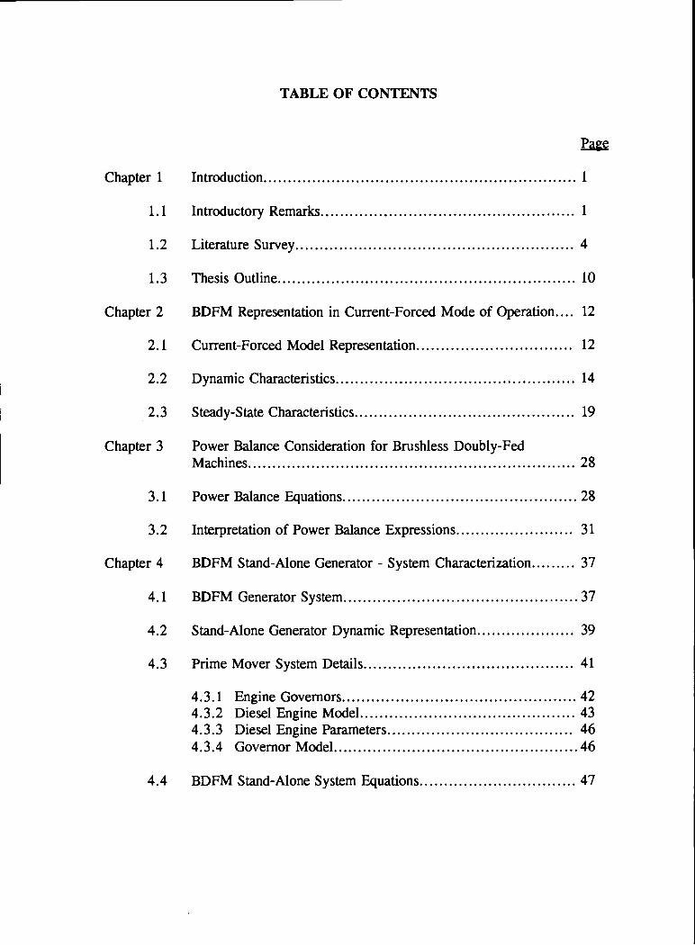
TABLE OF CONTENTS
Page
Chapter 1 Introduction ................................................................ 1
1.1 Introductory Remarks .................................................... 1
1.2 Literature Survey ......................................................... 4
1.3 Thesis Outline............................................................. 10
Chapter 2 BDFM Representation in Current-Forced Mode of Operation.... 12
2.1 Current-Forced Model Representation ................................ 12
2.2 Dynamic Characteristics................................................. 14
2.3 Steady-State Characteristics............................................. 19
Chapter 3 Power Balance Consideration for Brushless Doubly-FedMachines................................................................... 28
3.1 Power Balance Equations ................................................ 28
3.2 Interpretation of Power Balance Expressions........................ 31
Chapter 4 BDFM Stand-Alone Generator - System Characterization......... 37
4.1 BDFM Generator System ................................................ 37
4.2 Stand-Alone Generator Dynamic Representation.................... 39
4.3 Prime Mover System Details........................................... 41
4.3.1 Engine Governors................................................ 424.3.2 Diesel Engine Model ............................................ 434.3.3 Diesel Engine Parameters ...................................... 464.3.4 Governor Model .................................................. 46
4.4 BDFM Stand-Alone System Equations................................ 47

TABLE OF CONTENTS (Continued)
Page
Chapter 5 BDFM Stand-Alone Generator Steady-State Characteristics.... 50
5.1 Steady-State Representation ............................................. 50
5.2 System Characteristics ................................................... 51
5.2.1 Different Load Power Factors................................. 525.2.2 Different Operating Speeds..................................... 555.2.3 Simulated vs Experimental Results........................... 56
5.3 Issues of the System Sizing ............................................. 61
5.4 Case Study ................................................................. 62
Chapter 6 Linear Models and Stability Studies................................... 66
6.1 Linearized Models........................................................ 67
6.1.1 Complete Model .................................................. 676.1.2 Simplified Model ................................................. 736.1.3 Characteristic Equation ......................................... 75
6.2 Stability Studies ........................................................... 76
6.2.1 Comparing Simplified Model withCharacteristic Equation ......................................... 78
6.2.2 Changes in Eigenvalues with Load Current ................. 806.2.3 Changes in Eigenvalues with Load Power Factor .......... 81
Chapter 7 Stand-Alone Generator System Dynamic Characteristics........ 83
7.1 Open Loop Characteristics .............................................. 84
7.2 Closed Loop System Regulation using P1 Control.................. 87
7.2.1 Closed Loop Voltage Regulation Alone...................... 877.2.2 Closed Loop Voltage and Frequency Regulation ........... 92
7.3 Closed Loop System Regulation using Fuzzy Control ............. 93
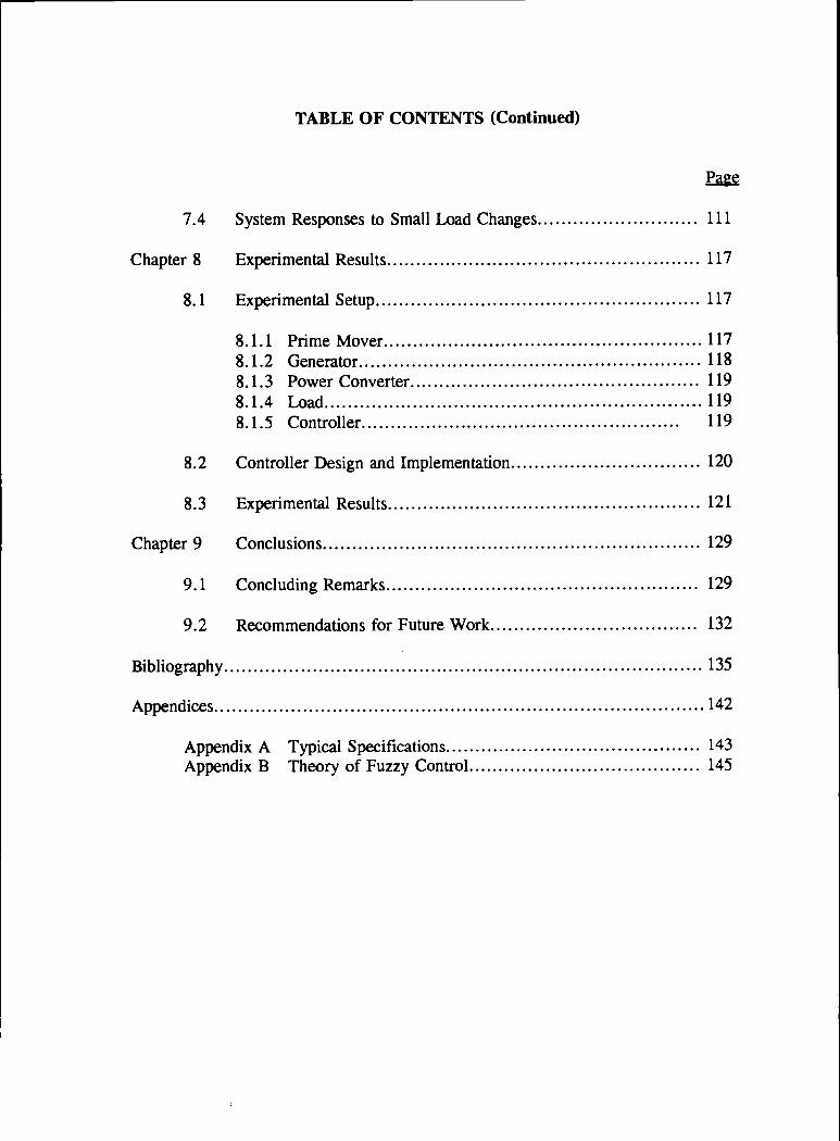
TABLE OF CONTENTS (Continued)
7.4 System Responses to Small Load Changes ........................... 111
Chapter 8 Experimental Results..................................................... 117
8.1 Experimental Setup....................................................... 117
8.1.1 Prime Mover ...................................................... 1178.1.2 Generator .......................................................... 1188.1.3 Power Converter................................................. 1198.1.4 Load ................................................................ 1198.1.5 Controller...................................................... 119
8.2 Controller Design and Implementation ................................ 120
8.3 Experimental Results..................................................... 121
Chapter 9 Conclusions................................................................ 129
9.1 Concluding Remarks ..................................................... 129
9.2 Recommendations for Future Work ................................... 132
Bibliography ................................................................................. 135
Appendices ................................................................................... 142
Appendix A Typical Specifications ........................................... 143Appendix B Theory of Fuzzy Control ....................................... 145

LIST OF FIGURES
Figure Page
1.1 Brushless Doubly-Fed Machine Drive System ................................ 3
1.2 Brushless Rotating Excitation System .......................................... 6
2.1 Equivalent Circuits for the Current-forced, Two-axis Modelin the Rotor Reference Frame ................................................... 15(a) q-axis Equivalent Circuit(b) d-axis Equivalent Circuit
2.2 Speed Response During Start-up and Synchronization ...................... 16
2.3 Power Winding q-axis Current Waveform During Start-upand Synchronization ............................................................... 17
2.4 Rotor q-axis Current Waveform During Start-up and Synchronization.. 18
2.5 Simulated Load Torque Profile .................................................. 19
2.6 Speed Responses During Sudden Load Changes ............................. 20(a) Voltage-Fed Mode Operation(b) Current-Fed Mode Operation
2.7 Torque Responses During Sudden Load Changes ............................ 21(a) Voltage-Fed Mode Operation(b) Current-Fed Mode Operation
2.8 BDFM Steady-state Equivalent Circuit (All Quantities at thePower Winding Frequency ....................................................... 24
2.9 Comparison of Power Winding Stator Currents .............................. 26
2.10 Comparison of Stator Power Factors ........................................... 27
3.1 Power Flow Diagrams ............................................................ 33(a) High-Speed Range, Generating Mode(b) Low-Speed Range, Motoring Mode
3.2 Power Balance in Motoring Mode at Constant Torque ..................... 35
4.1 BDFM Stand-Alone Generator System Block Diagram ..................... 38

LIST OF FIGURES (Continued)
Figure Page
4.2 Basic Engine-Governor System .................................................. 43
4.3 Engine-Governor System Speed-droop Profile................................ 48
5.1(a) Excitation Current Under Different Load Conditions ....................... 53
5.1(b) Excitation Voltage Under Different Load Conditions ....................... 53
5.2(a) Active Excitation Power Under Different Load Conditions ................ 54
5.2(b) Reactive Excitation Power Under Different Load Conditions............. 54
5.3 Mechanical Torque Required Under Different Load Conditions .......... 55
5.4 Mechanical Torque Required Under Different Speed Conditions......... 56
5.5(a) Excitation Current Under Different Speed Conditions...................... 57
5.5(b) Excitation Voltage Under Different Speed Conditions ...................... 57
5.6(a) Active Excitation Power Under Different Speed Conditions ............... 58
5.6(b) Reactive Excitation Power Under Different Speed Conditions ............ 58
5.7 Laboratory BDFM - Open Loop Magnetization Curve ..................... 60
5.8 Comparison of Experimental and Simulated Excitation Requirements 60
7. la,b Open Loop Characteristics Under Start-up .................................... 85
7. lc,d Open Loop Characteristics Under Load ....................................... 86
7.2 P1 Control Scheme in Block Diagram Form .................................. 88
7.3 Start-up Transients with Voltage Regulation Alone (PT Control) .......... 89
7.4 Transients Under Load with Voltage Regulation Alone (P1 Control).... 90
7.5 Changes in Frequency with Voltage Regulation Alone (P1 Control)..... 91

LIST OF FIGURES (Continued)
Figure Page
7.6 Voltage Transients Under Start-up (P1 Control) .............................. 94
7.7 Frequency Transients Under Start-up (PT Control) .......................... 95
7.8 (a) Q-axis Current ................................................................. 96(b) A-phase Current ............................................................... 96
7.9 Voltage Transients Under Load (P1 Control) ................................. 97
7.10 Frequency Transients Under Load (PT Control) .............................. 98
7.11 (a) Q-axis Current ................................................................. 99(b) A-phase Current ............................................................... 99
7.12 Voltage Regulation Fuzzy Membership Functions ......................... 103
7.13 Frequency Regulation Fuzzy membership Functions ...................... 104
7.14 Voltage Transients Under Start-up (Fuzzy Control) ......................... 106
7.15 Frequency Transients Under Start-up (Fuzzy Control) ...................... 107
7.16 Voltage Transients Under Load (Fuzzy Control) ............................ 108
7.17 Frequency Transients Under Load (Fuzzy Control) ......................... 109
7.18 Equivalent Phase-plane Plots at Start-up ....................................... 110
7.19 Simulated Load Profile ........................................................... 112
7.20 Voltage Transients for Small Load Disturbances (P1 Control) ............ 113
7.21 Frequency Transients for Small Load Disturbances (P1 Control) ......... 114
7.22 Voltage Transients for Small Load Disturbances (Fuzzy Control) ........ 115
7.23 Frequency Transients for Small Load Disturbances (Fuzzy Control).... 116
8.1 Experimental Setup Block Diagram.......................................... 118

LIST OF FIGURES (Continued)
Figure Page
8.2 Pulse to Analog Signal Conversion Circuitry................................. 121
8.3(a) Transient Responses of Voltage Regulation at Start-up (RMS Values).. 123
8.3(b) Transient Responses of Voltage Regulation at Start-up (Inst. Values)... 123
8.4 Transient Responses of Frequency Regulation at Start-up.................. 124
8.5 Terminal Voltage Waveform Under No-load Condition .................... 125
8.6(a) Transient Responses of Voltage Regulation Under Load (RMS Values). 126
8.6(b) Transient Responses of Voltage Regulation Under Load (Inst. Values). 126
8.7 Transient Responses of Frequency Regulation Under Load................ 128
8.8 Terminal Voltage & Current Waveforms Under Load Condition ......... 128
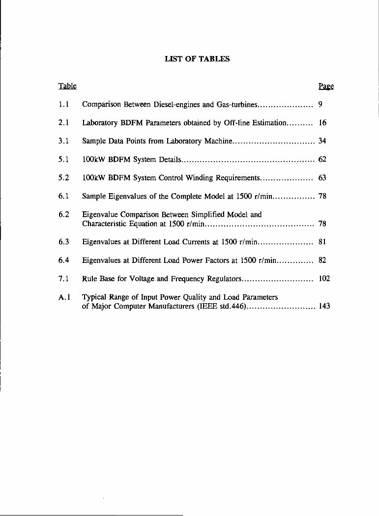
LIST OF TABLES
Table Page
1.1 Comparison Between Diesel-engines and Gas-turbines..................... 9
2.1 Laboratory BDFM Parameters obtained by Off-line Estimation.......... 16
3.1 Sample Data Points from Laboratory Machine............................... 34
5.1 100kW BDFM System Details.................................................. 62
5.2 100kW BDFM System Control Winding Requirements .................... 63
6.1 Sample Eigenvalues of the Complete Model at 1500 r/min ................ 78
6.2 Eigenvalue Comparison Between Simplified Model andCharacteristic Equation at 1500 r/min......................................... 78
6.3 Eigenvalues at Different Load Currents at 1500 r/min ..................... 81
6.4 Eigenvalues at Different Load Power Factors at 1500 r/min .............. 82
7.1 Rule Base for Voltage and Frequency Regulators........................... 102
A. 1 Typical Range of Input Power Quality and Load Parametersof Major Computer Manufacturers (IEEE std.446).......................... 143

LIST OF APPENDIX FIGURES
Figure Page
B. 1 (a) Normal Set ....................................................................... 146(b) Fuzzy Set....................................................................... 146
B.2 Max-Mm Composition in Graphical Form .................................... 149
B.3 Typical Fuzzy Control System .................................................. 149
Main Symbols
V,I
r
L
s,1,m
T
v,i
p,c,r
R
P
p
M
Re, Im
q, d
-
z
NOMENCLATURE
Voltage, Current Phasors
Resistance
Inductance
Subscripts for Self, Leakage and Magnetizing Terms
Electromagnetic Torque
Voltage, Current rms Quantities
Subscripts for Power winding, Control winding and Rotor
circuits
Subscript for Synchronous Frequency
Power
Pole Pairs
Angular Frequency
Mutual Inductance
Conjugate
Real, Imaginary Terms
Subscripts for Q-axis and D-axis Terms
Superscripts for Positive and Negative Sequence Terms
Impedance

Definitions
Power Winding Frequency
Control Winding Frequency
Rotor Angular Frequency
Rotor Electrical Frequency (Synchronous
Frequency)
P, = Re(V ) : Power Winding Electrical Power
p1 = . j2 Power Winding Copper Losses
P) = Re{jwpM.pIpIr Power Winding Air gap Power
= Re{V'I} : Control Winding Electrical Power
= ri2 : Control Winding Copper Losses
= Re(jwM0IIj : Control Winding Air-gap Power
Mechanical Power
P1.1 = r1.i2 : Rotor Circuit Copper Losses
= co,-p,1 = w+pc1 : Synchronous Frequency
= I : Slip with respect to Power Winding Field
S =I
: Slip with respect to Control Winding Field
S = : Total Slip in the Machine

Analysis of Brushless Doubly-Fed, Stand-Alone Generator Systems
Chapter 1
Introduction
The objective of this thesis is to introduce a novel, stand-alone generator system
which uses the Brushless Doubly-Fed Machine (BDFM). The main issues of interest
are the generator characteristics under steady state operating conditions, which in turn
gives an idea of the system component rating; and the stand-alone system dynamic
characteristics and control, under start-up and sudden load change conditions.
Specifically, the novelty of the system viz., generator terminal frequency control along
with the terminal voltage control, for varying prime mover operating speed, is to be
studied. Studies of BDFM modelling in the current-forced mode of operation and
analysis of the power balances in a BDFM pave the way for the stand-alone system
characterization and analysis.
1.1 Introductory Remarks
Stand-alone generator systems are used in a wide variety of situations e.g.,
lighting, transportation, mechanical utility systems, HVAC, industrial production, data
processing, life support and life safety systems, communication systems and signal
circuits.
In conventional stand-alone generator systems which use synchronous
generators, the output voltage is regulated by changing the dc field excitation and the
output frequency is controlled by maintaining the rated speed of the prime mover.

Thus, the generator output frequency regulation depends on the governor that is
connected to the prime mover. Even though simple mechanical governors are used in
some applications, expensive fixed-speed/electronic governors are commonly used to
maintain the speed of the prime mover in applications where frequency as well as
voltage needs to be tightly controlled under dynamically-changing load conditions.
Recent research has illustrated the advantages of the brushless doubly-fed
machine in adjustable-speed drive (ASD) and variable-speed generation (VSG)
applications and has shown the BDFM to be a viable alternative for selected
applications [1-4].
The BDFM operates in a mode similar to the doubly-fed, wound-rotor induction
machine, but has two stator windings on a single machine frame and a modified cage
rotor [5-6]. Fig. 1.1 shows the BDFM drive system configuration. The main stator
winding (power winding) has more pole pairs (Pr) than the auxiliary stator winding
(control winding) (Pa). When used in an ASD or a VSG, the BDFM realizes the
benefits of a conventional ac induction machine and has the advantages of reduced size,
rating, losses and cost of the power conversion unit which is used to excite the control
winding. The BDFM exhibits a synchronous operating mode in which two stator
excitations combine to produce a single rotor frequency at an intermediate mechanical
speed. In this mode, the BDFM operates as a synchronous machine with the control
winding providing the excitation. In the synchronous mode of operation, the amount
of power processed through the control winding is only a fraction of the total input
electrical power to the machine (output electrical power in the generator mode)

3
CONTROLLEDFREQUENCY
'IC
iCONVERTER
CONTROL WINDINGS
bidirectional
POWERFREQUENCY
-- - - pole-pairs
':'UTILITY I
POWE'I ROTOR
SUPPLY
.-P pole-pairs
-r- ,/(Pe+Pc) nests
---
Fig. 1.1. Brushless Doubly-Fed Machine Drive System
resulting in less converter loss than in a conventional ac drive and a substantial
reduction in capital costs.
In synchronous operation as an ASD or VSG connected to a power grid, the
shaft speed of the BDFM can be controlled by adjusting the frequency in the control
winding, while the power winding is connected to the utility supply (see Fig. 1.1). The
rotor mechanical frequency, is given by Eqn. 1.1; where f and f are the applied
stator frequencies. The positive and negative signs apply for positive and negative
sequences of the control winding excitation, with respect to the power winding
sequence.
f±f (1.1)r

4
The frequency and excitation levels of the control winding excitation, together
with the shaft velocity set by the prime mover dictate the output frequency and voltage
of the BDFM in the stand-alone generating mode of operation. This fact brings about
the novelty in using the BDFM as a stand-alone generator.
Since the output frequency can be controlled on the BDFM generator by using
control winding excitation, unlike conventional, non-electronic systems where the prime
mover system is responsible for frequency control, the proposed BDFM system can use
simple, inexpensive mechanical governors, resulting in reduced cost of the prime mover
system. The closed-loop control of the output frequency using the BDFM control
winding will be faster than in the case of a synchronous-machine system, where the
frequency depends on the shaft-speed dynamics of the prime mover system, which is
dominated by longer mechanical, rather than shorter electrical, time constants. Also,
by incorporating both the output voltage and frequency controls in a single unit on the
generator side, the generator system can be portable and can be used with a wide
variety of prime movers.
1.2 Literature Survey
IEEE std. 446-1980 (IEEE Orange Book) [7] defines a standby power system
as follows:
"An independent reserve source of electrical energy which, upon failure or outage of
the normal source, provides electrical power of acceptable quality and quantity so that
the user's facilities may continue in satisfactory operation".
[1
The same standards book defines an emergency power system as follows:
"An independent reserve source of electric energy which, upon failure or outage of the
normal source, automatically provides reliable electric power within a specified time
to critical devices and equipment whose failure to operate satisfactorily would
jeopardize the health and safety of personnel or result in damage to property".
One can also use the above-mentioned systems as the primary source of
electrical energy in remote operations.
There is very limited literature available on the topic of standby power systems,
which can be divided into two categories; viz., rotary and static standby systems. Most
of the literature on "rotary standby power systems" is focused on how to transfer the
load to the standby system when the normal source of power fails. The "static standby
power systems" consist of the batteries along with the power inverters that are required
to convert dc power to ac power. Because of their capability to operate continuously
on line, affording no break in power when the primary source fails, these static power
systems have been designated as Uninterruptible Power Supplies (UPS).
Combination of both rotary and static systems have been reported [8] and one
can classify them as "converter-based stand-alone power systems". The systems based
on synchronous generators often use the rotary converter (motor-generator set) as a post
conditioner for a simple, rugged inverter that can operate either from the rectified
utility power or batteries to provide regulated sinusoidal power. On the other hand,
systems based on cage-rotor induction generators use series-connected, ac-ac power
converters to generate the regulated sinusoidal power [9-10]. These systems cost higher
and have better dynamic regulation of the terminal quantities than the conventional,
synchronous-machine based systems.
Most of the standby or emergency systems use a synchronous generator as the
main electrical device. As mentioned earlier, the generator terminal voltage is regulated
by controlling the field excitation. There are various ways (with or without brushes)
of providing the dc excitation to the alternator field [11-12], but the most popular
excitation system is the brushless rotating excitation system with a solid state regulator.
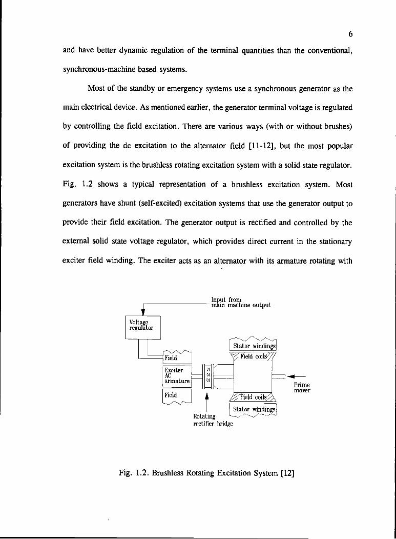
Fig. 1.2 shows a typical representation of a brushless excitation system. Most
generators have shunt (self-excited) excitation systems that use the generator output to
provide their field excitation. The generator output is rectified and controlled by the
external solid state voltage regulator, which provides direct current in the stationary
exciter field winding. The exciter acts as an alternator with its armature rotating with
Voltageregulator
Input frommain machme output
ield coi
Exciter
armature Primemover
Rotatingrectifier bridge
Fig. 1.2. Brushless Rotating Excitation System [12]
7
the main generator shaft. A shaft-mounted, full-wave rectifier bridge then converts the
exciter output to a dc supply, which supplies the main generator field winding.
The voltage regulator monitors the generator output voltage and accordingly
regulates the field excitation. In most of the cases, generator voltage alone is used as
the input to the excitation system. In order to obtain an improved response, some
excitation systems utilize the generator current signal as well. The current signal is
applied directly to the exciter without passing through the voltage regulator. This
provides fast response, especially under short-circuit or large motor starting conditions
when the voltage is low but the current is high.
Some of the voltage regulation methods result in an intentional voltage reduction
("browning out") when the load exceeds the prime mover output. Here a frequency-
sensing voltage regulator provides voltage reduction in proportion to frequency
decreases. This allows the system to regain rated frequency operation. This method
sometimes compromises the normal voltage regulation.
There are two main varieties of rotary standby systems from the point of view
of the prime movers engine-driven and turbine-driven.
Among the engine-driven systems, the diesel-engine is the most popular prime
mover. In reality, the diesel engine was the only prime mover used until the single-
shaft gas turbine (well known for its high-power output and small size) was developed
in 1961. Since then, gas-turbine generators are competing well with diesel-driven
systems, especially in the medium to high power range.
There are two varieties of turbine-driven generators; viz., steam-turbines and
gas/oil-turbines [7].

E1
Steam-turbines are used to drive generators which are larger than those which
can be driven by diesel engines. However, steam turbines are designed for continuous
operation. Also, steam turbines are expensive because they need a boiler with a fuel
supply and a source of water.
Most common turbine-driven electric generator units employed today for
standby systems use gas or oil for fuel. Kenney et aL, [13] discussed a 750kW gas
turbine-alternator system, which was designed for use as standby power in telephone
offices. The gas turbine is very sensitive to system disturbances while the diesel engine-
generator unit has a much slower dynamic response.
Table 1.1 compares the advantages and disadvantages between diesel-engines
and gas-turbines.
It was mentioned earlier that, in conventional standby systems, the generator
frequency response depends on the prime mover speed. A governor is used to maintain
a constant or nearly-constant engine speed (thereby, the generator frequency) by
automatically adjusting the engine fuel linkage under varying load conditions. There are
two varieties of governors and they are briefly discussed in Chapter 4. Diesel engine
and gas turbine governors are normally either hydraulic or electric. A hydraulic
governor senses speed with revolving flyweights and employs a hydraulic actuator to
operate the fuel linkage. An electric governor senses speed with either a frequency
sensor connected to the generator output or a rotating magnetic speed sensor. Load
sensing is available in some governors. Speed response is faster with this feature
because the load sensor, by monitoring current and voltage, senses load changes before
they have time to seriously affect system speed.
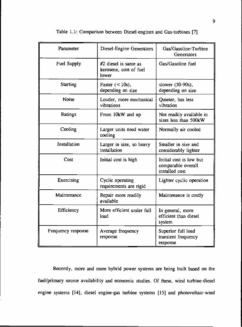
Table 1.1: Comparison between Diesel-engines and Gas-turbines [7]
Parameter Diesel-Engine Generators Gas/Gasoline-TurbineGenerators
Fuel Supply #2 diesel is same as Gas/Gasoline fuelkerosene, cost of fuellower
Starting Faster (<lOs), slower (30-90s),depending on size depending on size
Noise Louder, more mechanical Quieter, has lessvibrations vibration
Ratings From 10kW and up Not readily available insizes less than 500kW
Cooling Larger units need water Normally air cooledcooling
Installation Larger in size, so heavy Smaller in size andinstallation considerably lighter
Cost Initial cost is high Initial cost is low butcomparable overallinstalled cost
Exercising Cyclic operating Lighter cyclic operationrequirements are rigid
Maintenance Repair more readily Maintenance is costlyavailable
Efficiency More efficient under full In general, moreload efficient than diesel
system
Frequency response Average frequency Superior full loadresponse transient frequency
response
Recently, more and more hybrid power systems are being built based on the
fuel/primary source availability and economic studies. Of these, wind turbine-diesel
engine systems [14], diesel engine-gas turbine systems [15] and photovoltaic-wind

ID]
systems are important. In most of these studies, the primary issues are the transient
stability analysis and the dynamics of interaction between the two sources.
In a standby system, when there is a sudden load impact, the generator supplies
the initial power demand by using the energy stored in its magnetic field. This is
because the generator rotor angle does not change instantly with load demand; so
energy is not instantly recovered from that stored in the rotating masses. Thus, a
mechanical storage device (buffer), such as a fly-wheel, is usually required between
any critical load and the standby generators to compensate for any deviations in the
generator terminal quantities caused by sudden load changes. Once the rotor angle
changes due to the loading, the stored energy in rotating parts can be used for
supplying the power demand.
Appendix A lists a typical range of input power quality and load parameters
specified by computer manufacturers. These specifications are taken as the basis in
designing the system control requirements throughout this work.
1.3 Thesis Outline
The objective of this work is to introduce the BDFM as a stand-alone generator
system. Of particular interest are the studies on modeling and characteristics of the
proposed generator system.
Firstly, in Chapter 2, the current-forced model of the BDFM is introduced. The
model facilitates a simplified approach to system understanding and control. Chapter
3 briefly deals with the air-gap power balance analysis of the BDFM. This study is
done to better understand the BDFM system in the motoring and generating modes of
operation.

11
Chapter 4 introduces the stand-alone generator system characterization and
models, both for the BDFM and the diesel engine with a simple mechanical governor.
Chapter 5 consists of the steady state representation of the stand-alone system
and presents characteristics under different load conditions. Also, a case study has been
included to highlight the information which can be obtained from this representation.
Chapters 6 and 7 consist of the dynamic control and stability issues concerning
the stand-alone system. Linearized models, which are useful for small-signal stability
studies of non-linear systems, are developed.
Chapter 8 explains some of the experimental results obtained using the
laboratory prototype BDFM under start-up and sudden load changes and proves the
feasibility of the BDFM stand-alone generator system. Chapter 9 lists the conclusions
of this work and gives directions for some future work on the BDFM stand-alone
generator systems.

12
Chapter 2
BDFM Representationin Current-Forced Mode of Operation
This chapter discusses the development of a current-forced model for a brushless
doubly-fed machine (BDFM). The term "current-forced" refers to the BDFM operation
with a power converter operating in the current-command mode connected to the
control winding terminals.
2.1 Current-Forced Model Representation
It is well known that dynamic analysis of electric machinery can more readily
be carried out in the d-q axis reference frame. The initial dynamic equations for the
BDFM were first written in a rotor-reference frame in the d-q domain by Li [16]. The
rotor-reference frame is chosen in order to eliminate the time-varying terms in the
inductance matrix of the dynamic equations.
The dynamic and steady-state BDFM models were developed and analyzed by
Li et al., [16] and later modified by Boger et aL, [17]. In these BDFM model
representations, it was assumed that both stator windings are excited by voltage sources
as shown in Fig. 1.1. The zero-sequence variables of a balanced, 3-phase system are
zero. Using this assumption, the BDFM equations in the d-q domain are given by Eqn.
2.1. This voltage-forced system is a sixth order electrical system. Since the BDFM has
nested rotor bars short-circuited at an end-ring on one side, the rotor voltages Vqr and
Vd are equal to zero.
13
vqj, r+L,p PPLSp(*)r 0 0 MprP PM1co1 i
v, r+L,p 0 0 PpMprCir M1p i11,
v 0 0 r+Lp PcL,Wr -M1p PcMcr()r 1qc (2.1)0 0 r+L,p PcMcr(z)r M1p
Vqr MprP 0 McrP 0 rr+Lrp 'qr
Vdr 0 M1p 0 M 0 r1+L1p 1dr
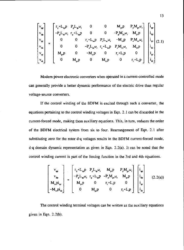
Modern power electronic converters when operated in a current-controlled mode
can generally provide a better dynamic performance of the electric drive than regular
voltage-source converters.
If the control winding of the BDFM is excited through such a converter, the
equations pertaining to the control winding voltages in Eqn. 2.1 can be discarded in the
current-forced mode, making them auxiliary equations. This, in turn, reduces the order
of the BDFM electrical system from six to four. Rearrangement of Eqn. 2.1 after
substituting zero for the rotor d-q voltages results in the BDFM current-forced mode,
d-q domain dynamic representation as given in Eqn. 2.2(a). It can be noted that the
control winding current is part of the forcing function in the 3rd and 4th equations.
vcii, [r+L,p PPLSpWr M p P M Wpr p prr
1
qp1
[dPIvI
PpMprWr MprPI
(2.2(a))McrPqc
I
M1p 0 rr+Lrp 0i
lqrI
L_MPLi [0 MprP 0 rr+Lrp j [idj
The control winding terminal voltages can be written as the auxiliary equations
given in Eqn. 2.2(b).

10 r+L,p PL,w1 McrP PCMCrCr
0 -PLo, r +Lp PM@ McrP
'dp
1qc
'dc
'qr
'dr
14
(2.2(b))
Figure 2.1 shows the two-axis diagram representation of the current-forced
BDFM in the rotor reference frame based on Eqn. 2.2. It can be noticed that the
control winding self inductance, L,, and resistance, r are not explicitly present in this
representation.
This current-forced model representation of the BDFM [18], while retaining all
the information pertaining to machine dynamics, is a reduced order model which
simplifies the analysis of machine characteristics, stability and control.
2.2 Dynamic Characteristics
In order to obtain the dynamic characteristics of the BDFM in the current-forced
mode, the BDFM electrical system equations as given in Eqn. 2.2 have to be solved
simultaneously with the mechanical system equations as given in Eqn. 2.3 [16].
P(Or) =P(°'r) = T TL ko, (2.3)
T, = Pp 'tpr (lqp 'dr 'dp q1) + p Mcr (qc 'dr + 'dc qr)
where J is the moment of inertia and k is the viscous damping coefficient.
Simulation studies are performed using Eqns. 2.2 and 2.3. For the sake of
continuity with respect to the earlier work, as well as to enable comparisons with the

15
PwM i PwLiprprdr prspdp
(a) q-axis Equivalent Circuit
PwM i PwLIprprqr prspqp
(b) d-axis Equivalent Circuit
Fig. 2.1. Equivalent Circuits for the Current-forced, Two-axis Model in the RotorReference Frame

16
Table. 2.1: Laboratory BDFM Parameters obtained by Off-line Estimation
Paia.ni R(0)
L(mH)
MJR(s)
R(0)
L(mH)
Mcr/Rr
(s)Lr/R.(s)
Value 0.7 0.049 0.0027 1.8 0.247 0.0338 0.194
experimental data, a BDFM with 6/2 stator pole combination is used. Table 2.1 gives
the prototype BDFM parameters obtained by off-line parameter estimation in the
laboratory [19]. The off-line estimation procedure estimates some of the parameters in
the form of ratios instead of absolute values. Thus, the value of the rotor resistance is
taken to be 0.000330 from theoretical calculations; and the mutual inductances and
rotor self inductance are calculated accordingly.
100
N80
60
I
0+-0.0 0.2 0.4 0.6 0.8 1.0
Thne (s)
Fig. 2.2. Speed Response During Start-up and Synchronization

17
Figure 2.2 shows the simulated BDFM start-up speed response to
synchronization under no-load conditions. At t = Os, a voltage of 230V at 60Hz is
applied to the power winding; and a nominal negative sequence current of 5A at 5Hz
is applied to the control winding for BDFM motoring operation. The machine reaches
a synchronous speed of 825 r/min (13.75Hz) as predicted by Eqn. 1.1.
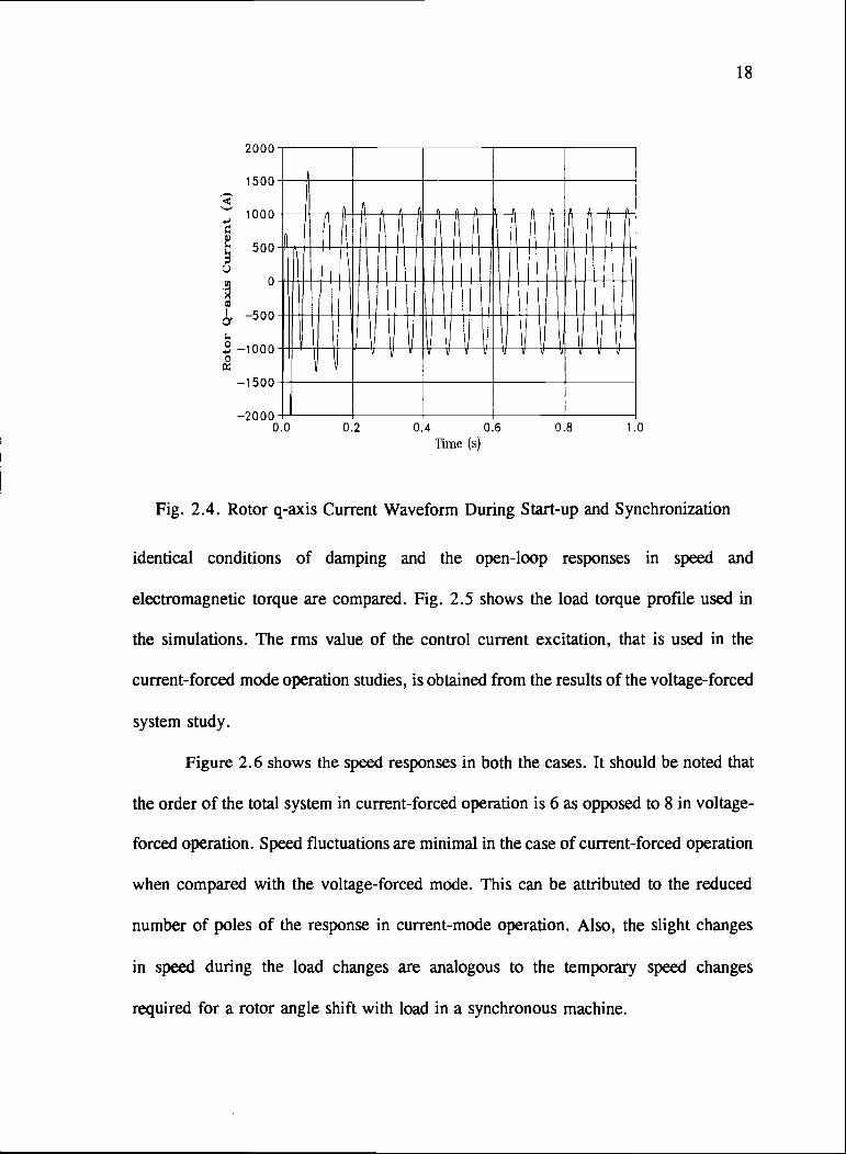
Figure 2.3 shows the simulated q-axis current in the power winding during start-
up and synchronization. Fig. 2.4 shows the rotor circuit q-axis current for the same
conditions.
In order to evaluate the advantages of current-forced operation, simulation
comparisons are made between the voltage-forced model and the current-forced model.
An identical load torque profile is applied to both the models, at t = 2.5s, under
60
40
20
I I
t.I
. 20
400.0 0.2 0.4 0.6 0.8 1.0
Time (s)
Fig. 2.3. Power Winding q-axis Current WaveformDuring Start-up and Synchronization
18
2000
1500
1000
500
10& 500
10000
1500
2000 -F-0.0 0.2 0.4 0.6 0.8 1.0
Time (s)
Fig. 2.4. Rotor q-axis Current Waveform During Start-up and Synchronization
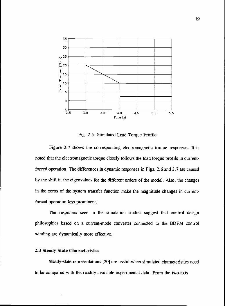
identical conditions of damping and the open-loop responses in speed and
electromagnetic torque are compared. Fig. 2.5 shows the load torque profile used in
the simulations. The rms value of the control current excitation, that is used in the
current-forced mode operation studies, is obtained from the results of the voltage-forced
system study.
Figure 2.6 shows the speed responses in both the cases. It should be noted that
the order of the total system in current-forced operation is 6 as opposed to 8 in voltage-
forced operation. Speed fluctuations are minimal in the case of current-forced operation
when compared with the voltage-forced mode. This can be attributed to the reduced
number of poles of the response in current-mode operation. Also, the slight changes
in speed during the load changes are analogous to the temporary speed changes
required for a rotor angle shift with load in a synchronous machine.
35
30
_. 25
20
0
10
5 -F--
2.5 3.0 3.5 4.0 4.5 5.0 5.5
Time (s)
Fig. 2.5. Simulated Load Torque Profile
19
Figure 2.7 shows the corresponding electromagnetic torque responses. It is
noted that the electromagnetic torque closely follows the load torque profile in current-
forced operation. The differences in dynamic responses in Figs. 2.6 and 2.7 are caused
by the shift in the eigenvalues for the different orders of the model. Also, the changes
in the zeros of the system transfer function make the magnitude changes in current-
forced operation less prominent.
The responses seen in the simulation studies suggest that control design
philosophies based on a current-mode converter connected to the BDFM control
winding are dynamically more effective.
2.3 Steady-State Characteristics
Steady-state representations [20] are useful when simulated characteristics need
to be compared with the readily available experimental data. From the two-axis

95
go
85
a)
80
0
75 +-2.5
95
90
a)
a)
C),
85
C)a)
80
0
0
75+-2.5
3.0 3.5 4.0 4.5 5.0 5.5
Time (s)
(a) Voltage-Fed Mode Operation
3.0 3.5 4.0 4.5 5.0 5.5
Time (s)
(b) Current-Fed Mode Operation
Fig. 2.6. Speed Responses During Sudden Load Changes
20

21
35
-30
''25
'20
. 15
5 +-2.5
35
30
Ei 25
a,
o 20I.-
0I-
15a,C
o 10E0I'-
a,w
0
5 -1---
2.5
3.0 3.5 4.0 4.5 5.0 5.5
Time (s)
(a) Voltage-Fed Mode Operation
3.0 3.5 4.0 4.5 5.0 5.5
Time (s)
(b) Current-Fed Mode Operation
Fig. 2.7. Torque Responses During Sudden Load Changes

22
dynamic equations, steady-state equations using the current-forced model are derived
by using the phasor notations suggested by P.C.Krause [21]. In the steady-state analysis
in the rotor reference frame, all the quantities are assumed to be at the induced rotor
frequency, 'R given by
= = (2.4)
where w is a radian frequency. R is the electrical frequency induced in the rotor
circuit. Rated synchronous speed of the BDFM is defined to be the speed with the
control winding excited at zero frequency (dc).
The symmetrical-component transformation [21] is used here to effectively treat
the issue of different excitation sequences in the stator windings in order to obtain the
phasor-domain, steady-state equations from the d-q domain expressions in Eqn. 2.2.
The d-q quantities are converted into positive and negative sequence quantities
by using the transformations
Fq = F + FFd = j(F F-)
(2.5)
where F can be a voltage(rms) or a current(rms). These symmetrical component
transformations lead to the following set of equations.
= (r+ic L )I + WpMpIrJ p sp p
i)RMCIC = jRMPI + (rf+jcoL)I (2.6)
T = 2 j(1 1 '-P 1) + 2PCMp p r p r C

23
The implication of the positive and negative sequences used in Eqn. 2.6 is that
the fundamental-frequency, air-gap MMF rotates in different directions in the two
different sequences. The control winding is represented by the negative sequence
quantities, because the negative sequence control winding direction of rotation is built
into the dynamic, d-q domain expressions that are used here.
Using the theory of symmetrical components, we can also write that, for
positive-sequence, balanced-stator excitation,
(2.7)
where represents the conjugate quantity. For negative-sequence, balanced-stator
excitation,
I- = ; P = 0 ; (2.8)
Substituting these values in Eqn. 2.6 and using the definition of the slip with respect
to the power winding field, we obtain the steady-state equations for the BDFM in
phasor-domain form as given below. It should be noted that these steady-state equations
are represented at the power winding frequency.
V, = (r +j I, + j CpVfpr
= iM1I + (.fL +JCApLr) I (2.9(a))
T = Re(ppMpjIp Ir)Similarly, Eqn. 2.2(b) results in the following steady-state equation representing
the control winding quantities.
* = (r +j I *+ j cMcrIr (2.9(b))

24
It should be noted that for balanced, poly-phase excitation, the per-phase,
equivalent circuit voltages and currents reduce to the actual rms phase voltages and
currents [22]. The per-phase equivalent circuit representation of the BDFM in the
steady-state condition, with all the quantities are at the power winding frequency, is
shown in Fig. 2.8, where
X4,,(L5, M);
X=
Xir' = (tp(Lr-Mpr); (2.10)= (J)pM,.
S =-.(J_,p
r iX;
IP
- - - -
JXI, I
r
VP
Fig. 2.8. BDFM Steady-state Equivalent Circuit (All Quantities at the PowerWinding Frequency)
25
It should be noted that current-forced excitation of the control winding is
reflected as a voltage-source in the circuit.
For steady-state analysis of the BDFM, the two phasor equations from the
equivalent circuit along with the torque expression should be considered. The set of
five non-linear equations in real algebraic form with the power winding voltage as the
reference are expressed in Eqn. 2.11.
= 0
rpi+pLspi+opMprin = 0
rn1.1 coLi. RMprhjp RMcrhic = 0 (2.11)
= 0
2P M (ii1.1.-i9,i11.)+2PM1(i i. -i. i )-T = 0IC II IC 11 Lp pr
This set of equations can be solved for the power winding current, rotor current
and the phase angle between power winding voltage and control winding current for
a given load and speed condition. All the voltages and currents are rms phase
quantities. In Eqn. 2.11, r and i used as first subscripts in the current terms refer to
the real and imaginary quantities.
Steady-state characteristics of the BDFM were simulated for the 6/2 stator pole
combination using the laboratory machine parameters and compared with the data
obtained from laboratory experiments. The machine was run at 825 r/min at a constant
torque of 11.3 Nm (100 lb/in). A series-resonant converter was used in the current-
source mode to provide the control winding current excitation.
Figure 2.9 shows the predicted and measured power winding current magnitude
with varying control winding current. This curve is analogous to the lagging section of
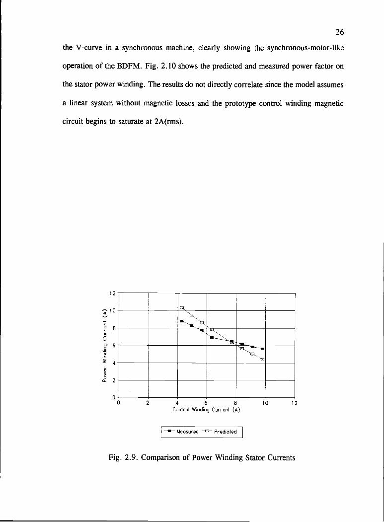
26
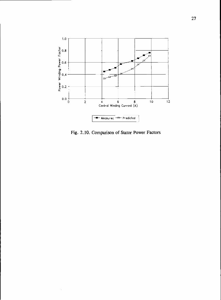
the V-curve in a synchronous machine, clearly showing the synchronous-motor-like
operation of the BDFM. Fig. 2.10 shows the predicted and measured power factor on
the stator power winding. The results do not directly correlate since the model assumes
a linear system without magnetic losses and the prototype control winding magnetic
circuit begins to saturate at 2A(rms).
12
'10
C
-uC
0-f0 2 4 6 8 10 12
Control Winding Current (A)
Measured Predicted
Fig. 2.9. Comparison of Power Winding Stator Currents
I00
CC
Fig.
°fltro wifld9 C(Jrreflt (A
/TII
Comparison °f Stat

28
Chapter 3
Power Balance Considerationsfor Brushless Doubly-Fed Machines
While the viability of the BDFM in selected applications is well established, it
is important to note the power distribution between the stator windings and the rotor
circuit to better understand the machine for various speed and load conditions. In
singly-fed and wound-rotor induction machines, the power flow between the stationary
and the rotating sections passes the air-gap only once in a given direction for a given
mode of operation; the expressions for the amount of power in each section are simple
and well understood [31-32].
In the case of the BDFM, power crossing the air gap is provided by two
separate sources, leading to a model with two terms, rather than one; so additional
analysis is necessary to obtain the power distribution between the stator windings and
the rotor circuit. This power distribution analysis will help, not only during the design
process of the machine, but also in deciding on the converter rating for a specific
application with a given speed range and load profile.
3.1 Power Balance Equations
For the sake of completeness in the analysis of the BDFM power balance, the
steady-state voltage equation corresponding to the control winding terminals as given
in Eqn. 2.9(b) is also considered along with the current-forced steady-state model as
described in Eqn. 2.9(a).
29
The following points are to be noted before deriving the power balance
expressions for the BDFM:
S The low-speed region is defined as the speed below the BDFM rated
synchronous speed;
The transition-speed region is defined as the speed above the BDFM rated
synchronous speed and below the synchronous speed of the power winding
field;
The high-speed region is defined as the speed above the synchronous speed of
the power winding field;
c is defined to be positive for speeds below the rated synchronous speed and
negative for speeds above;
All losses except copper losses are neglected
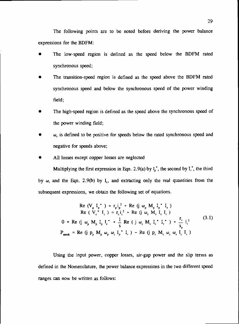
Multiplying the first expression in Eqn. 2.9(a) by J,, the second by Ir*, the third
by w, and the Eqn. 2.9(b) by I, and extracting only the real quantities from the
subsequent expressions, we obtain the following set of equations.
Re (\' I, ) = ri2 + Re (j M I I )Re ( V ) = r i2 + Re (j w M I Ir )
r (3.1)O=Re(jw MI 'r .Re(jwMI Ir)+_r2
S S
'incch = Re (j p M w1, r [p Ir ) Re (j PC M 'c 'r [c Ir )
Using the input power, copper losses, air-gap power and the slip terms as
defined in the Nomenclature, the power balance expressions in the two different speed
ranges can now be written as follows:

Low-Speed Range:
P = P1 + p(ag)p p
= 'c1 'c(ag) (3.2)= I I 'p(ag) Sc 'c(ag)
'mech = (1 Is I) 'p(a) (1 c(ag)
Transition-Speed Range:
High-Speed Range:
Pp = Ppi + Pp0g
= cl + "c(ag) (3.3)'ri = I Sp I 1'p(aS) c "c(ag)
'mech = (1 IsI) P + (1 + 'c(ag)p(ag)
= + 'p(ag)
= 'cl + 'c(ag) (3.4)Pr! = _ISpI P + S Pp(ag) c c(ag)
'mech = (1+ s,, I) P + (1 s) c(ag)p(as)
Combining equations 3.2 through 3.4 into a single representation, we obtain the
expressions which represent the power balance in a BDFM, either in the motoring or
generating modes and over the complete speed range of operation. These expressions
are given by
= + 'p(ag)
= cl + (3.5)'rl cp '3p(ag) F S 'c(ag)
'mch = (1 s) p(ag) (1 'c(ag)

31
The negative sign is used for speeds below the rated synchronous speed and the positive
sign for speeds above the rated synchronous speed.
In a wound rotor induction machine (WRIM), neglecting losses, the expressions
for the power balance are given by [31],
P, = s, Pg (3.6)'mech = (1 s) P
where P1 is the slip power, Pg is the air gap power and 5md is the slip in the induction
machine.
Comparing the expressions in 3.5 and 3.6, it is noted that the power flow
through the stator power and control windings with respect to the rotor in a BDFM is
represented by expressions similar to those in a wound rotor induction machine, with
additional complexity. A simple analysis of the power distribution is given in the next
section.
3.2 Interpretation of Power Balance Expressions
By considering proper sequences and proper definitions of the slip terms in
different speed regions, it can easily be shown that the control winding air gap power,
as defined in Nomenclature, has a negative value in the low-speed region and a positive
value in the high-speed region. This results in the control winding delivering power to
the supply line, through the power converter, during low-speed motoring and high-
speed generating modes of operation. These modes of operation are analogous to the
slip-power recovery of wound-rotor induction machines. Conversely, additional power

32
needs to be supplied to the machine through the control winding in low-speed
generating and high-speed motoring.
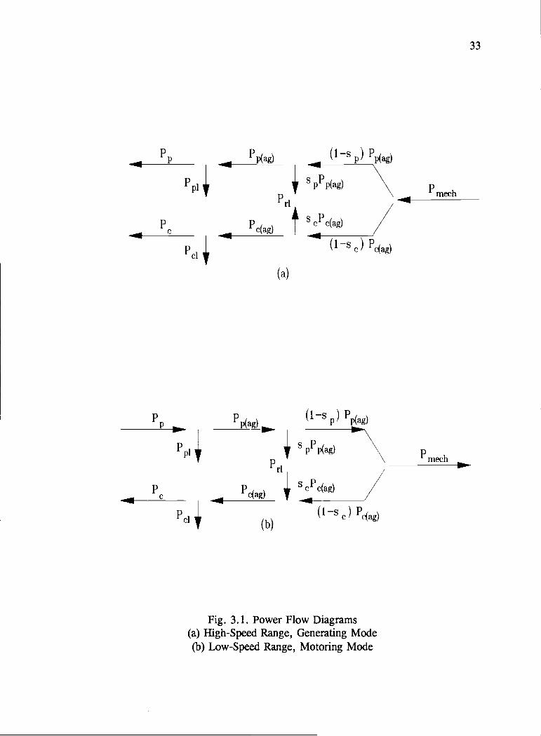
Fig. 3.1 shows the power flow diagrams of the BDFM in low-speed motoring
and high-speed generation considering only the resistive losses. For a given mode of
operation, the direction of power flow is represented based on the signs of the power
terms in Eqn. 3.5, after substituting the proper expressions for the slip terms. P1, P
and P.1 are the copper losses in the stator and the rotor circuits. In Fig. 3.1(a), the input
mechanical power, after accounting for the rotor losses, crosses the air gap as two
electrical power terms, corresponding to the power in the two stator windings.
Similarly, in Fig. 3.1(b), the input power from the stator main winding is divided
between the output mechanical power and the regenerative control winding electrical
power. The proportional amounts of power distribution and the amount of copper losses
in different circuits depend on the speed and the mode of operation of the machine.
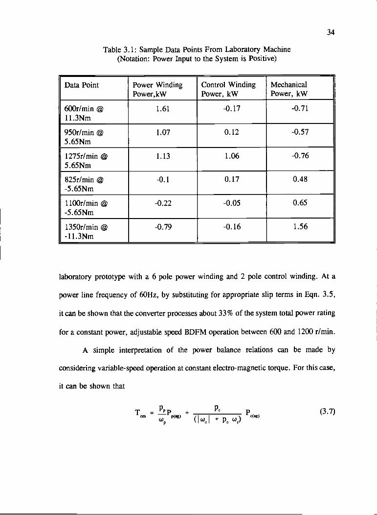
A 5kW laboratory prototype BDFM having a 3/1 stator pole pair combination
has been built and tested. Sample test data points obtained from the experiments are
given in Table 3.1. The negative torque (positive mechanical power with respect to the
BDFM power winding) values correspond to BDFM generator operation and the
positive torque (negative mechanical power) values indicate the motoring mode. The
rated synchronous speed of this machine is 900 r/min. Different terminal power data
points are presented for motoring and generating modes. The data points show that the
trend in power distribution is as expected from the expressions given in Eqn. 3.5.
The converter rating for a particular application can be obtained by substituting
proper terms in the set of expression given in Eqn. 3.5. For example, consider the
Pp
33
PC
P
pC
'p(ag) (1s ) Pp(g)p
r1
SpPp(ag)
c(ag)cc(ag)
(1se) c(ag)
(a)
mech
(1s ) 'p(ag)ag)
s'mech
r1
ag)cc(ag)
(1se) e(ag)(b)
Fig. 3.1. Power Flow Diagrams(a) High-Speed Range, Generating Mode(b) Low-Speed Range, Motoring Mode
34
Table 3.1: Sample Data Points From Laboratory Machine(Notation: Power Input to the System is Positive)
Data Point Power Winding Control Winding MechanicalPower,kW Power, kW Power, kW
600r/min@ 1.61 -0.17 -0.7111. 3Nm
950r/min 1.07 0.12 -0.575.65Nm
1275r/min @ 1.13 1.06 -0.765.65Nm
825r/min @ -0.1 0.17 0.48-5. 65Nm
ilOOr/min -0.22 -0.05 0.65-5. 65Nm
1350r/min c -0.79 -0.16 1.56-11.3Nm
laboratory prototype with a 6 pole power winding and 2 pole control winding. At a
power line frequency of 60Hz, by substituting for appropriate slip terms in Eqn. 3.5,
it can be shown that the converter processes about 33 % of the system total power rating
for a constant power, adjustable speed BDFM operation between 600 and 1200 r/min.
A simple interpretation of the power balance relations can be made by
considering variable-speed operation at constant electro-magnetic torque. For this case,
it can be shown that
ppP (3.7)T,,,p(ag) (kI + p ')

35
Fig. 3.2 shows the relationship between the different normalized power
components in the BDFM as a function of speed for constant-torque motoring operation
between standstill and 900 r/min. In this simple representation, all the rotor losses are
neglected; but, in a practical case, the power relations are not linear and depend on the
loading condition; i.e., control winding regeneration can be noticed only beyond a
certain band about the rated synchronous speed ( after accounting for the control
winding copper losses), while motoring or generating in the low or high band of
operation, respectively. This is due to two reasons: the control winding terminals also
supply the magnetizing power required under light load conditions of the machine to
compensate for its losses; and part of the control winding regenerative power
contributes towards the control winding copper losses. It can be observed that the
1
-1
PrATLr (r ii'
Fig. 3.2. Power Balance in Motoring Mode at Constant Torque
(r/min)
combination of the two air gap powers produce the mechanical output power (input
during generation). At rated synchronous speed, the control winding has a dc
excitation; so no air gap power is processed through the control winding terminals. A
similar representation can be obtained for BDFM generator operation. From the figure,
it can also be noted that, for a limited speed range of 600-900 r/min, the power through
the control winding has a maximum value of about 33% of the total system rating.
This, however, does not address reactive power requirement, which will slightly raise
the converter rating.
Despite the simplifying assumptions made in the formulation of the power
balance expressions, the resulting representation gives a good indication of machine
characteristics and is a good starting point for design and development studies.

37
Chapter 4
BDFM Stand-Alone Generator- System Characterization
This chapter describes the characterization of a BDFM, stand-alone generator
system. Although the study described in this thesis is valid with most of the
conventional prime movers, a diesel engine is considered as the prime mover in this
study, primarily because the diesel engine is the most popular and an extremely robust
prime mover. Other prime movers viz., steam, hydro, wind etc., whose models are
given in [14,36] can also be used with a BDFM generator system.
4.1 BDFM Generator System
Figure 4.1 shows the block diagram of a BDFM, stand-alone generator system.
Throughout this study, the prototype BDFM as described in Chapter 2, is used. When
the BDFM is operated as a stand-alone generator, the electrical load is supplied through
the power winding terminals. This power is supplied by the prime mover through the
common shaft.
The control winding is used to provide excitation to the BDFM generator. The
control winding is connected to the generator output and to a separate source (which
can be a battery) through a power electronic converter. An auxiliary power supply
should be used to initially supply power to the control winding terminals. Instead of
connecting to the power winding terminals, a separate source is assumed for the control
winding excitation in this study.
In Chapter 3, it was shown that, in high speed BDFM generation, energy can
be extracted from or supplied to the control winding circuit depending on the speed and

38
/'DFM N\ Power'Widing
calPrime ferator
ConWindingi
I
ac<--->dcI
I
dc<--->acPower I PowerConverter I Converter
PowerConverter
AuxiliatySource
Fig. 4.1. BDFM Stand-Alone Generator System Block Diagram
load condition. In light of this fact, apart from the supply from the generator terminals,
a separate excitation source (rated higher than a regular auxiliary source) for the
control winding can be beneficial for the following reasons:
S By using a separate source for control winding excitation, energy can be
supplied to the BDFM generator load on a short-term basis when the load
demands are higher than that provided by the prime mover; and energy can be
returned to the separate source under light load conditions. This operation is not
possible in conventional generators where all the active power comes from the
prime mover alone. This additional energy can be supplied to the load either
through the machine air-gap or directly through the power converter.
S It was mentioned that in a conventional, stand-alone generator system, the
prime mover takes a finite period before it responds to sudden load changes.

Even with fast acting voltage regulators, the dynamic responses of the terminal
quantities suffer due to the non-availability of energy to instantly supply the
demand. This drawback does not arise when a separate excitation method is
used in a BDFM generator; because the sudden demand in load can be
compensated by the control winding before the prime mover responds to the
load change. Thus the resultant transient responses of the terminal quantities in
a BDFM generator will be superior to those of conventional systems and qual
to that provided by the converter-based systems.
S Also, the reactive power to the load can be supplied directly through the
power converter stage connected to the power winding terminals, instead of
through the machine air-gap. This operation will increase the system efficiency.
4.2 Stand-Alone Generator Dynamic Representation
Equation 2.2 gives the BDFM dynamic equations in the current-forced mode of
operation. In this representation, since the BDFM is being used as a stand-alone
generator now, the voltages at the power winding terminals are to be taken as outputs
instead of forcing functions. Thus, the voltages need to be written in terms of the
currents and the operational load impedance [33].
Let the load impedance at power winding frequency in the Laplace domain be
ZL = RL + sLL (4.1)
where RL is the load resistance and LL is the load inductance.
By considering the terminal quantities, in the abc domain, the terminal voltage
can be represented as

40
[v] = LL [ + R [jb](4.2)
dt L
But, it was mentioned earlier that the BDFM dynamic representation, as given
in Eqn. 2.2, is in the rotor reference frame; so Eqn. 4.2 cannot be used direcfly for
substituting the power winding d-q voltage terms.
The transformation matrix used to transform the power winding a-b-c quantities
into d-q quantities is given by Li, et al. in [16].
obtain
cos(30r) COs(30 120°) cøs(30+ 120°)
[C1I = %/(2/3) sin(30r) sin(301-120°) sin(301+120°) (4.3)
V(112) I(1/2) 1(1/2)
By using this transformation, and by premultiplying the Eqn. 4.2 by [Cpr], we
di (4.4)[Cpr] [v] = RL [C,1] Uabc] + LL [Cr1] ]
The second term in Eqn. 4.4 can be modified by substituting the following
expression.
[_iqp
[Cr1] [.f][dlqdO]
3r I
dp I
(4.5)dt
LoJ
In the resultant expression, the term {LL(dqd,Idt)} is small when compared with
the term {3LLi} (except, perhaps, at light loads). Thus, for balanced source and

41
load conditions, after neglecting the term {LL(dqdjdt)}, the power winding d-q voltage
terms can be represented as follows:
[Vq = RL Uq + 3 LL H 1 (4.6)['dj
In the above equation, the negative sign is used; because the power winding terminals
are treated as load terminals instead of source terminals.
After substituting the above equations in Eqn. 2.2(a), the generator equations
in the stand-alone mode are given as follows:
[ o 1 Fr+R+L,p 3Lsp()r+XL MprP 3MprWrl [iqp1
I0 XL3Lsp(t)r r+R+LSp 3Mprr M1p (4.7)IMti.Pq
IMpi.P 0 r+Lp 0
I qr
L_Mci'jL
0 MprP 0 r1Lp] LU
It can be observed that the expression represents a fourth order system with two
forcing functions provided by the control winding currents.
4.3 Prime Mover System Details [7, 14,34-36J
Conventionally, different prime movers; viz., gas turbines, steam turbines,
water turbines, windmills, dual fuel and spark-ignited gas engines and diesel engines,
are used in stand-alone generator systems. Diesel-generator systems are well
investigated and are well established. This section considers a BDFM stand-alone
system with a diesel engine as the prime mover.
The diesel engine is a very complex device for which it is very difficult to write
a comprehensive mathematical model. However, the complex models are required

42
mostly for large-signal transient analysis. A small-signal model is sufficient for dealing
with small-to-moderate, sudden changes in load conditions.
4.3.1 Engine Governors
In a prime mover, a constant, or near constant, speed is achieved by using
speed regulators, popularly known as governors. Most of the prime movers, mentioned
above employ governors, often much the same units as used in diesel systems but each
has its own peculiarities and requirements. There are two important varieties of
governors:
(a) Permanent, Speed-Droop Governor: The speed droop is a measure of the
speed change necessary to cause the governor's control shaft to travel through its full
working range. Since an increase in fuel is required if the engine is to carry more load,
it follows that an increased load requires a decrease in speed. The typical allowable
speed droop is 3 to 5 percent of the rated engine speed.
In most of the systems with the permanent, droop-type governor, the engine's
speed is slightly higher at light loads than at heavy loads, within a desired nominal
speed at full load.
(b) Temporary Speed-Droop Governor: This governor is also known as an
'isochronous' governor. In the governor, the output shaft will always come to rest at
the same speed, so that the engine's final steady speed remains constant regardless of
load. Normally, under steady state, frequency tends to vary slightly above and below
the normal frequency setting of the governor. The extent of this variation is a measure
of the stability of the governor. An isochronous governor should maintain frequency
regulation within ±1/4 percent. When load is added or removed, speed (and frequency)
43
dips or rises momentarily. One to three seconds are usually required for the governor
to cause the engine to settle at a steady state at the new load. Expensive electronic
governors are used for this type of regulation.
Either of the aforementioned governors can be used for the BDFM stand-alone
systems. For the initial feasibility study of the BDFM stand-alone generator system and
to prove the economic viability of the proposed system, the permanent speed-droop
governor will be used.
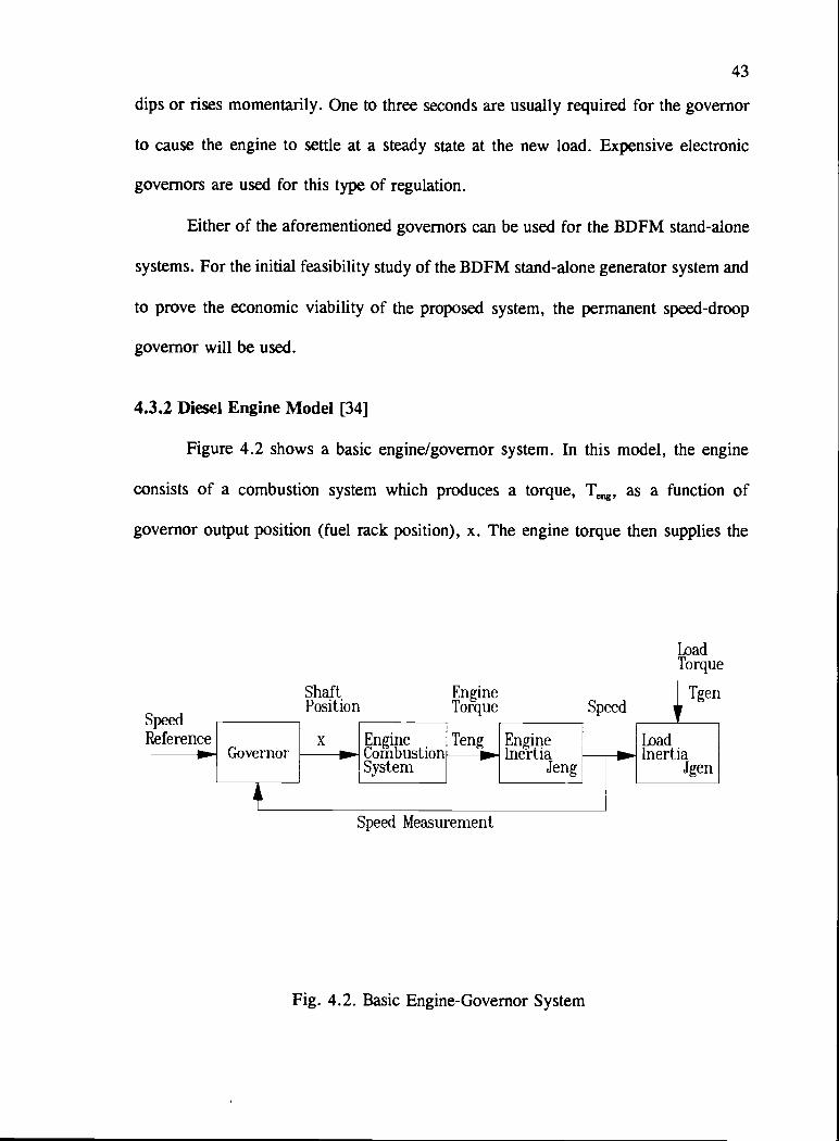
4.3.2 Diesel Engine Model [34]
Figure 4.2 shows a basic engine/governor system. In this model, the engine
consists of a combustion system which produces a torque, T, as a function of
governor output position (fuel rack position), x. The engine torque then supplies the
EnginePosition Torque Speed
SpeedReference x Engine Teng Engine
Governor Combustion inertiaSystem Jeng
Speed Measurement
Fig. 4.2. Basic Engine-Governor System
LoadTorque
Tgen
LoadInertia
Jgen

44
load torque, Tg, and any difference between these two torques will help accelerate or
retard the system.
If, when running at equilibrium, the load setting of the engine is changed by a
small amount Tg and the engine is governed such that the fueling rate and
subsequently the governor output position is changed by &, then the new equilibrium
point achieved is associated with a small speed change &.
and
Letting
then
The final, incremental changes in torque are given by:
For equilibrium
(aT) (3T) (4.8)eng 00
ôTgen = (4.9)
= (4.10)
(3Tgen)= A;
ÔT( = B; ( ) = k1 (4.11)
gen
(A B) = k1 ox LTgen (4.12)

45
This equation shows the steady state speed change resulting from small changes
in governor shaft position and generator loading condition.
Dynamically, during the transition between equilibrium points the torque
imbalance will act on the rotating inertia as described by:
Bow0 + k1Ox LTgen A&,0 = J._(&) (4.13)
which can be represented as
kOx= I gen (4.14)
° JD + (A-B)
where d/dt is represented as D. This is the simple basic transfer function for a
governed engine on load as given by [34].
Also, in a diesel engine, there is a time delay between the action of the
governor in demanding a change in fuelling rate and the response of the engine to that
change. The effective firing delay has been found empirically to be the actual time
between consecutive pistons arriving at the injection point plus approximately a quarter
of a revolution of the crankshaft.
The effective firing delay for the condition is given by
60s 60Tf (4.15)
where s is the number of strokes in an engine, N is the speed in r/min and n represents
the number of engine cylinders.

46
The complete transfer function of a governed engine on load, along with the
firing delay, is given by
k1 e -T Dox
JD + (A-B)(4.16)
4.3.3 Diesel Engine Parameters
The following parameters, obtained by scaling down the parameters of a 100KW
engine [34], are used for the diesel engine throughout the simulation studies:
Number of Cylinders : 4
Number of Strokes : 4
Total Inertia : 2 kg.m2
Full Load Power : 10 kW
Rated Speed : 1500 r/min (157.08 rad/s)
Governor Shaft Length : 5 mm
Firing Delay : 0.03 s
Full Load Torque : 63.662 Nm
Acceleration Rate : 20 %/s
Torque/Rack Gain : 21.221 Nm/mm
Torque/Speed Slope : -0.18 Nm/rad/s
4.3.4 Governor Model [34,36]
A simple mechanical governor with a permanent speed-droop characteristic is
used in this section. The objective is to show that, even with a simple governor, we can
obtain good dynamic response of the generator terminal voltage and frequencies.

47
In a simple mechanical governor, the centrifugal force on two or more weights
rotating about an axis driven by the engine is balanced against either gravity or a
spring. Any change in speed of rotation shifts the balance position of the mechanism
and the movement is transmitted via a linkage to the fuel valve of the engine; thus
effecting control of the speed of rotation. The discussion on the details of the governor
is out of the scope of this thesis, even though the author has used the transfer function
pertaining to the governor which is given by Eqn. 4.17 as shown below [34,35].
-0.48&; D2 2D +1 (4.17)
where x is the throttle position and w represents speed. The equation depends on
several parameters of the mechanical governor viz., total mass of the fly balls, friction,
spring stiffness etc., This governor system can be used in conjunction with the diesel
engine whose parameters are given in section 4.3.3.
The governor has a fixed speed setting of 1500 r/min; and is designed in such
a way that the speed droop is about 5.2% for a 20 Nm change in engine load.
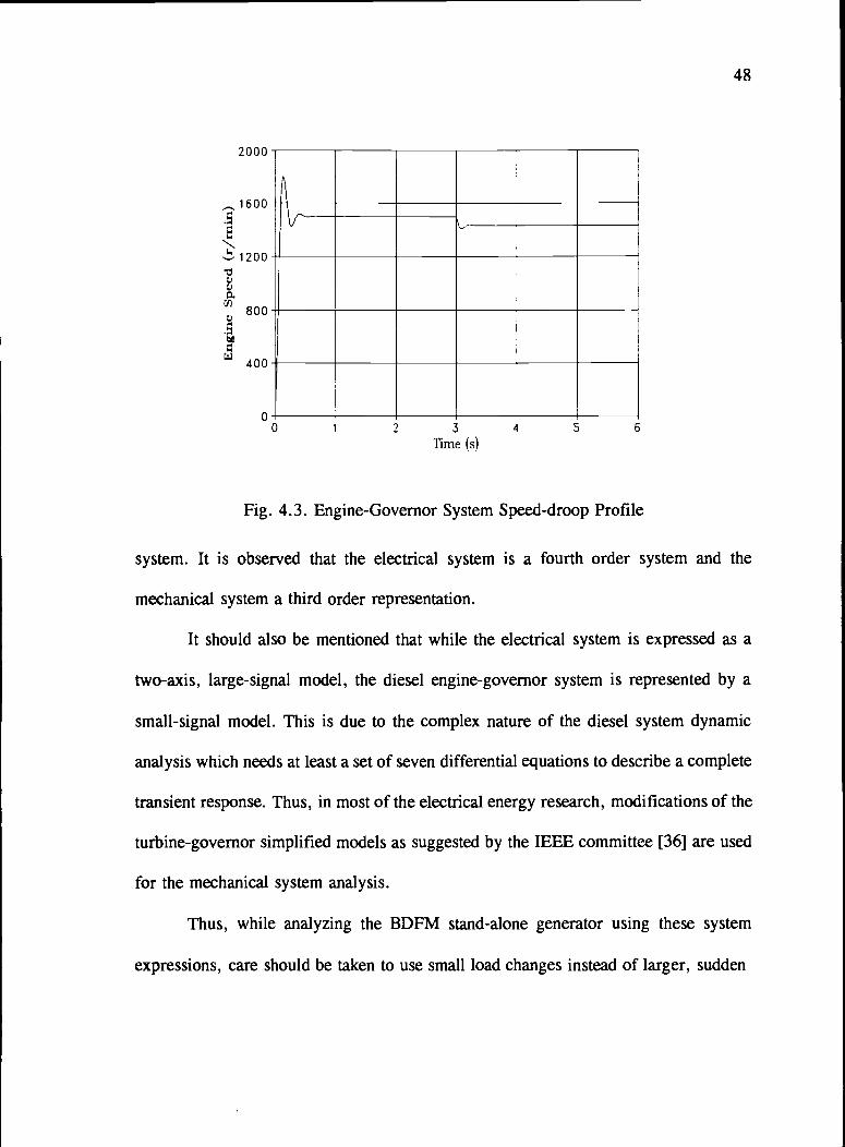
Figure 4.3 gives the speed-droop profile of the combined engine-governor
system defined in Section 4.2.2.1. Initially the engine is allowed to start under no-load
and the speed reaches the rated speed of the engine. At t = 3s, a sudden load of 20
Nm is applied to the mechanical system and the speed settles at 1422 r/min.
4.4 BDFM Stand-Alone System Equations
The BDFM stand alone generator system with a diesel engine as the prime
mover can be completely represented by Eqns. 4.7, 4.16 and 4.17. This is a 7th order
48
2000
1600
N1200
800
400
0+0 1 2 3 4 5 6
Time (s)
Fig. 4.3. Engine-Governor System Speed-droop Profile
system. It is observed that the electrical system is a fourth order system and the
mechanical system a third order representation.
It should also be mentioned that while the electrical system is expressed as a
two-axis, large-signal model, the diesel engine-governor system is represented by a
small-signal model. This is due to the complex nature of the diesel system dynamic
analysis which needs at least a set of seven differential equations to describe a complete
transient response. Thus, in most of the electrical energy research, modifications of the
turbine-governor simplified models as suggested by the IEEE committee [36] are used
for the mechanical system analysis.
Thus, while analyzing the BDFM stand-alone generator using these system
expressions, care should be taken to use small load changes instead of larger, sudden

49
load changes. Also, the analysis should always be done around some operating point
with the load changes resulting in small speed deviations.

50
Chapter 5
BDFM Stand-Alone Generator- Steady-State Characteristics
This section presents the steady state characteristics of the BDFM stand alone
generator system. The characteristics are analogous to those of a synchronous generator
driven by any prime mover (The nature of the prime mover is inconsequential during
the steady state studies). In a BDFM generator, the ac excitation requirements should
be carefully considered due to the converter rating dependence on the reactive
excitation power requirements.
5.1 Steady-State Representation
Section 4.1.1 describes the dynamic representation of the BDFM stand-alone
generator in the two-axis domain. From the stand-alone system equations given in Eqn.
4.7 and the torque expression given in Eqn. 2.3, by using the symmetrical component
transformation, the following phasor expressions can be obtained (in the process of
converting the instantaneous quantities to rms quantities, a factor of V'2 is used, which
changes the torque equation from Eqn. 2.3 to the form as shown below):
0 = (r + ZL + j cL,) I + j (*pMpI
iWRMcrIc = JC)RMprIp + (r + JR"rY'r (5.1)
2ppMprIm[I I 1 + 2pMIm[-II1J Tmc,h = 0pr-'
where a high-speed range BDFM generator operation is chosen. Tmh is considered
negative for generator operation.

51
The synchronous frequency induced in the rotor is given by
= Ppr = (5.2)
The auxiliary expression representing the control excitation voltages is given by
-V = (r jo,L) i J)cMcrIr (5.3)
The above equations can now be solved simultaneously to obtain the steady state
characteristics. By assuming the phase angle of the rated power winding voltage to be
zero at different load impedances for a given load power factor, we can obtain the load
current values. One can then solve Eqn. 5.1 for the following quantities: (1) excitation
current phasor, (2) rotor current phasorr; and (3) mechanical torque required to
supply power to the load, Tmh. The excitation voltages can then be calculated using
Eqn. 5.3; and subsequently, the excitation power requirements can be calculated in
deciding the converter rating. Also, the phase angle between V, and I, gives the
direction of power flow. In a high-speed BDFM generator, the value is more than 900,
indicating regenerative power through the control winding.
5.2 System Characteristics
Simulated BDFM steady-state characteristics were obtained in stand-alone mode
operation by using parameters of the laboratory machine as given in Chapter 2, Table
2.1. These characteristics will be helpful in obtaining the ratings of different
components of the stand-alone system under different operating conditions. Some of the
simulated results are compared with laboratory results.

52
5.2.1 Different Load Power Factors
The simulated load conditions assume a generator terminal voltage of 230V
(rms) at 60Hz under all load conditions. Results are obtained for different load current
values at different load power factors ranging from O.8(lead) to O.4(lag).
Figure 5.1 shows the excitation current and voltage requirements. As is the case
with a synchronous generator, for a similar load current, the required excitation current
increases while the load power factor deteriorates (from leading pf towards the lagging
pf loads). On the contrary, the excitation voltage requirement slightly goes up as the
load power factor improves towards the leading power factor conditions.
In a stand-alone system under normal operating conditions, the active load
power is supplied by the prime mover and the reactive power by the control excitation
system. Fig. 5.2 shows the active and reactive power requirements at the control
winding terminals. It can be seen that the reactive power requirements (Fig. 5.2(b))
decrease with improving load power factors since the required reactive compensation
from the control winding is decreased. Also, a slight increase is observed in active
power as load power factor improves from low lagging pf values to higher lagging pf
values. This active power is a regenerative power through the control winding.
It should be noted that as the load power factor decreases, the total power
output of the system decreases with a constant voltage at the generator terminals and
at a given load current condition. Fig. 5.3 gives the total mechanical power
requirement under different load conditions. With improving load power factor, the
system is delivering more active power at the rated voltage and at a fixed load current
and thus the required mechanical torque also increases in a linear fashion.
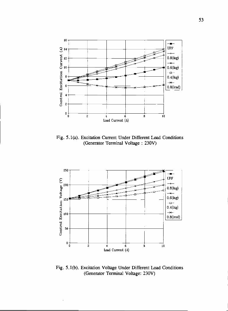
53
16
i4
12
o 10
C
C0
0 2 4 6 8 10
Load Current (A)
UPF-p-O.8(Iag)
0 .6 (lag)
0.4(lag)
0.8(Iead)
Fig. 5.1(a). Excitation Current Under Different Load Conditions(Generator Terminal Voltage: 230V)
250
200
150
0 100
50
C0
00
-UPF
0.8(lag)
0.6(Iag)-8-0. 4 (lag)
0.8(lead)
2 4 6 8 10
Load Current (A)
Fig. 5.1(b). Excitation Voltage Under Different Load Conditions(Generator Terminal Voltage: 230V)

54
1750
1500
1250
10000
750C)
500
250
00
-UPF
O1ag)
O1ag)
OA1ag)
ø;!1__->-----
- -44--
O.8(lead)
4 6 6 10
[i)ad Current (A)
Fig. 5.2(a). Active Excitation Power Under Different Load Conditions(Generator Terminal Voltage: 230V)
750
600
450
300
150
00
UPF
O.8(lag)
O.6(lag)
I
______-
OAlag)
O.8(Iead)
2 4 6 8 10
load Current (A)
Fig. 5.2(b). Reactive Excitation Power Under Different Load Conditions(Generator Terminal Voltage: 230V)
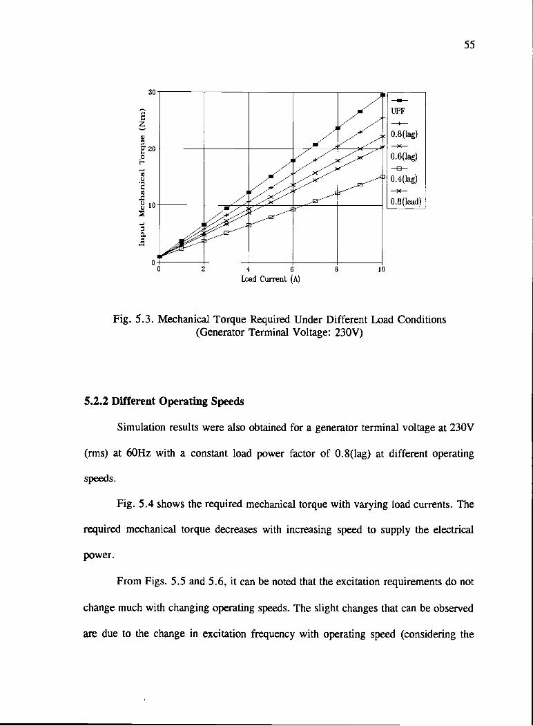
55
30
z
20
19
4.?
10
040 2 4 6 8 10
Load Current (A)
UPF
0 .8 (lag)--0 .6 (lag)-B-0. 4 (lag)
0.8(lead)
Fig. 5.3. Mechanical Torque Required Under Different Load Conditions(Generator Terminal Voltage: 230V)
5.2.2 Different Operating Speeds
Simulation results were also obtained for a generator terminal voltage at 230V
(rms) at 60Hz with a constant load power factor of O.8(Iag) at different operating
ss.Fig. 5.4 shows the required mechanical torque with varying load currents. The
required mechanical torque decreases with increasing speed to supply the electrical
power.
From Figs. 5.5 and 5.6, it can be noted that the excitation requirements do not
change much with changing operating speeds. The slight changes that can be observed
are due to the change in excitation frequency with operating speed (considering the

56
30
20
0
10
4,
00 2 4 6 8 10
load Current (A)
1500 r/min
1350 r/min
1850 r/min
Fig. 5.4. Mechanical Torque Required Under Different Speed Conditions(Generator Terminal Voltage: 230V; Load pf: 0. 8(lag))
terminal frequency constant at 60Hz), and the subsequent changes in the control
winding impedances.
5.2.3 Simulated vs Experimental Results
Test results were obtained by using the laboratory machine described in Chapter
1. As mentioned earlier, the laboratory prototype machine is not designed for any
specific application. The initial tests revealed that the excitation requirements for
obtaining rated generator terminal voltage, 230V are very high, as is predicted in the
simulation studies. It was noted that the control winding inductance begins to saturate
at a current magnitude of about 2.5 A. Thus, even a very high current magnitude
results in a marginal increase in the flux contributed by the control winding. Also, the
laboratory series resonant converter that is being used to excite the control winding has

57
El
+ 12
09C
C
0 2 4 6 8 10
Ii)ad Current (A)
1500 r/min--1350 r/min
1650 r/min
Fig. 5.5(a). Excitation Current Under Different Speed Conditions(Generator Terminal Voltage: 230V; Load pf: O.8(lag))
200
150
Q 100
50
-
0 2 4 6 8 10
Ioad Current (A)
1500 r/min
1350 r/min
1650 r/min
Fig. 5.5(b). Excitation Voltage Under Different Speed Conditions(Generator Terminal Voltage: 230V; Load pf: O.8(lag))

11
1750
1500
1250
C
1000C
' 7500
500
250
00 2 4 6 0 10
Load Current (A)
1500 r/min
1350 r/min
1650 r/min
Fig. 5.6(a). Active Excitation Power Under Different Speed Conditions(Generator Terminal Voltage: 230V; Load pf: O.8(Iag))
800
600
C;; 400
4-,
2004-,
0
0
Load Current (A)
-1500 r/mm
1350 r/min
1650 r/min
Fig. 5.6(b). Reactive Excitation Power Under Different Speed Conditions(Generator Terminal Voltage: 230V; Load pf: O.8(lag))
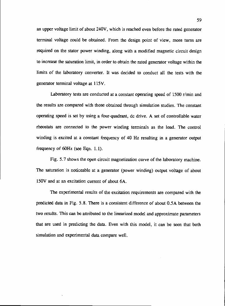
59
an upper voltage limit of about 240V, which is reached even before the rated generator
terminal voltage could be obtained. From the design point of view, more turns are
required on the stator power winding, along with a modified magnetic circuit design
to increase the saturation limit, in order to obtain the rated generator voltage within the
limits of the laboratory converter. It was decided to conduct all the tests with the
generator terminal voltage at 1 15V.
Laboratory tests are conducted at a constant operating speed of 1500 r/min and
the results are compared with those obtained through simulation studies. The constant
operating speed is set by using a four-quadrant, dc drive. A set of controllable water
rheostats are connected to the power winding terminals as the load. The control
winding is excited at a constant frequency of 40 Hz resulting in a generator output
frequency of 60Hz (see Eqn. 1.1).
Fig. 5.7 shows the open circuit magnetization curve of the laboratory machine.
The saturation is noticeable at a generator (power winding) output voltage of about
150V and at an excitation current of about 6A.
The experimental results of the excitation requirements are compared with the
predicted data in Fig. 5.8. There is a consistent difference of about 0.5A between the
two results. This can be attributed to the linearized model and approximate parameters
that are used in predicting the data. Even with this model, it can be seen that both
simulation and experimental data compare well.

200
150
4-,
100
E 50
0-F0 2 4 6 8 10
Excitation Current (A)
Fig. 5.7. Laboratory BDFM Open Loop Magnetization Curve
C..)
04-,
.1
0
12
8
4
0*0 4 8 12
Ioad Current (A)
-Experimental-F--
Simulated
Fig. 5.8. Comparison of Experimental and Simulated Excitation Requirements(Speed: 1500 r/min; Generator Terminal Voltage: 1 ISV)
61
5.3 Issues of the System Sizing [37]
In a BDFM stand-alone generator system, there are three major components,
namely, generator, prime mover and the power converter, that need to be chosen based
on the nature of the load.
While estimating the load, both the static as well as dynamic loads need to be
considered.
While considering the static loads, it is important to consider both the
power(kW) and kVAr rating of the loads because the prime mover is sensitive to power
or torque and the generator system is based on current or thermal effects.
Motor starting loads and any other loads which are suddenly applied for short
duration come under the category of dynamic loads. Unless such loads have very low
power factor values, the resulting thermal effect on the generator can be ignored.
Sizing for the transient load should be done on a worst case scenario and the auxiliary
components such as voltage and frequency regulators, governor system etc., should be
designed accordingly.
The active power (kW) demand of the system load should be met by the prime
mover, which in turn should be matched to the continuous maximum rating of the
generator. Also, the prime mover should be rated in such a way that the overload
capacity will not be exceeded as well as the transient speed droop is within the design
limits. In a diesel engine system, the short term output torque corresponds to the
fueling rate at the time of operation and maximum horsepower is limited by maximum
engine fueling because a diesel system does not have ability to store any energy beyond
the inertial energy.
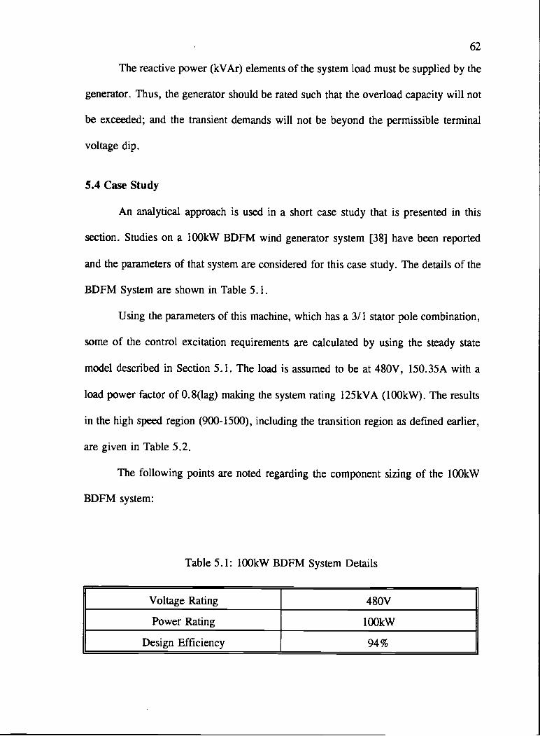
62
The reactive power (kVAr) elements of the system load must be supplied by the
generator. Thus, the generator should be rated such that the overload capacity will not
be exceeded; and the transient demands will not be beyond the permissible terminal
voltage dip.
5.4 Case Study
An analytical approach is used in a short case study that is presented in this
section. Studies on a 100kW BDFM wind generator system [38] have been reported
and the parameters of that system are considered for this case study. The details of the
BDFM System are shown in Table 5.1.
Using the parameters of this machine, which has a 3/1 stator pole combination,
some of the control excitation requirements are calculated by using the steady state
model described in Section 5.1. The load is assumed to be at 480V, 150.35A with a
load power factor of 0.8(lag) making the system rating 125kVA (100kW). The results
in the high speed region (900-1500), including the transition region as defined earlier,
are given in Table 5.2.
The following points are noted regarding the component sizing of the 100kW
BDFM system:
Table 5.1: 100kW BDFM System Details
Voltage Rating 480V
Power Rating 100kW
Design Efficiency 94%

63
Table 5.2: 100kW BDFM System Control Winding Requirements(Load: 100kW, 480V, 150.35A, 0.8pf lag)
Speed, r/min [_Control Current,A Control Voltage,V kVA Rating
975 294.09 82.15 24. 162
1050 294.42 155.56 45.801
1125 295.80 270.03 79.877
1275 293.83 418.17 122.87
1350 293.43 452.43 132.76
1425 293.43 520.57 152.75
1500 293.45 594.12 174.35
It should be noted that the prime mover is to be rated to deliver 100kW active
power and a short term additional active power. The power winding stator should be
designed to process the rated load active power. In any case, the engine and the
generator have widely varying characteristics and ratings are often matched differently
for different applications. From the system sizing point of view, the main issue that
should be focused on, in the case of a BDFM stand-alone generator system, is the
overall power converter rating.
The advantage of using the doubly-fed machine in reducing the cost of the prime
mover system (using a simple governor) has been mentioned previously. Depending on
the load demand requirements, the prime mover and the generator are chosen. From
Table 5.2, it is noted that as the operating speed increases in the high speed region, the
control winding excitation requirements go up. In this case study, it can be concluded
that it is economical to operate the BDFM generator just above it's synchronous speed.
Correspondingly, a prime mover with a rated speed about this operating point should
be chosen.
As the operating speed increases, the kVA rating of the required power
converter increases; and, beyond a certain operating speed, the BDFM stand-alone
system loses economic advantage over the synchronous or induction generator-converter
based systems. It can be concluded that by operating this system in a speed range of
900-1200 r/min, a maximum converter rating of approximately 75% of the total system
rating is required and this system compares favorably against any converter based
stand-alone systems. By using proper gear boxes with a given prime mover system or
by choosing a prime mover system with appropriate rated speed, a favorable BDFM
operational speed can be chosen to make BDFM operation competitive.
It can also be noted that the required excitation current remains constant with
changing speed and the excitation voltage increases with increasing impedance. It can
be observed that for a 480V system (assuming that the control winding is also rated at
480V), this system cannot be operated beyond about 1400 r/min. In order to operate
the system in its complete high-speed range, the number of turns on the control
winding needs to be increased so that we can maintain the converter rating with
reduced current (which will reduce the converter cost as well) and increased voltage
requirements. But this fact complicates the machine design process and may result in
a bigger machine frame than that which is obtained with a regular design. This
indicates that BDFM stand-alone generators need application-specific, modified machine
design techniques.

65
Considering that a BDFM uses more copper than a conventional machine of
similar rating, this BDFM system can be competitive if the converter rating is kept
within a certain maximum rating which is a fraction of the total system rating. It is
demonstrated in this case study that this system is most viable for operating speeds
nearer to the synchronous speed value.

Chapter 6
Linear Models and Stabifity Studies
In order to study the system behavior when small perturbations are applied, non-
linear systems are linearized (first-order approximations are made) around an operating
point. In such cases the new and the old equilibrium operating points are nearly equal
and the new linearized equations are valid only about the quiescent condition [33].
In Chapters 2 and 4, the BDFM, d-q domain, stand-alone system equations are
represented in the rotor reference frame. Two types of nonlinearities appear: product
nonlinearities and trigonometric functions. To study issues regarding system control and
stability, these equations need to be linearized. One way of obtaining the linearized
equations is by using Floquet theory and Li [39] has used this method for stability
studies of the BDFM using the voltage-forced dynamic equations. A different approach
has been used in this study in obtaining the linearized model of the BDFM stand-alone
system.
The dynamic response of a linear system is determined by its characteristic
equation. The roots of this characteristic equation give the necessary information
regarding the system dynamic characteristics. In particular, the free response gives an
indication of the system stability.
Two approaches are used in obtaining stand-alone dynamic characteristics:
small-signal analysis about an operating point and simulation studies of a prototype
BDFM generator.
I In this chapter, linearized models for the BDFM stand-alone system are
derived and some results pertaining to the dynamics and stability of the system

are given. The equations of the BDFM stand-alone system derived in Chapter
4 are differential equations that describe system behavior as a function of time.
When the system operates in a steady-state condition, differential equations are
not necessary since all the variables are either constants or (in the case of
BDFM system) sinusoidal variations with time. One can assume all the variables
to be in a steady-state condition prior to a disturbance. The so-called small-
signal stability study deals with the system behavior following the disturbance.
The results from the BDFM system steady-state equations can be used as the
initial conditions that exist prior to the disturbance and then the small-signal
model can be used to obtain the information about system stability.
I Chapter 7 describes the system dynamics through simulation studies using a
prototype machine.
6.1 Linearized Models
The current-forced mode dynamic equations, along with the diesel engine
expressions, as given in Chapter 4, are considered in obtaining the system linearized
equations.
6.1.1 Complete Model
From Eqn. 4.7, the state space model of the BDFM stand-alone generator can
be obtained and is shown in Eqn. 6.1 (on next page) along with the electro-magnetic
torque equation, where k is given by
k = L, Lr Mpr2 (6.2)

!qp
'dpi1qr
'dr
Lr(rp +R1)
3L1(L +LL) r
M(r +RL)
3M1,(L1, L)r
L1
10I+-k
Mpr
0
3Lr(Lsp +L) (i)
Lr(rp +RL)
3M1(1, +LL)
M1,(r +R1)
oM1,1
C
Lr 0 -
oL1,
Mpr0
rM
3rLrMpr
30
0Pt
0 MJqc
L1, M!dC
3
3üM2
r1L,
Tern = p, M1 (qp ir
-ip qr) + Pc M1 (qc th + i i)
qp
'dp
'qr
'dr
(6.1)

Let us assume w is a state in the state-space representation. At the occurrence
of a small disturbance, let the state change by w from the initial equilibrium point w0.
Thus
w = + w4 (6.3)
Note that w0 need not be fixed, but should be a known value for the analysis of the
linearized model.
The state-space model in Eqn. 6.1, which is in the form
reduces to
when Eqn. 6.3 is applied.
w = f(w , t) (6.4)
*0 + * = f(w0-+-w , t) (6.5)
The states in the current-forced model of a BDFM generator can be written as
'qpo + 'qp
'dp = 'dpo +
1 1 (6.6)qr qro qr
'dr = 'ciro + dr4
= ro+
By substituting the expressions shown in Eqn. 6.6 in Eqn 6.1 and after
neglecting the second-order perturbation terms, one can now obtain the linearized
model of a BDFM generator as represented by the set of expressions in Eqn. 6.7 (P.
71).
70
The linearized representation of the diesel engine can be obtained directly from
the previous chapters. In Chapter 4, the 10kW diesel engine model along with the
mechanical governor model was represented in transfer function form. A state-space
model can easily be obtained from the transfer function form and is shown in Eqn. 6.8,
= z
+ 82 z + 1681 x = -42025 (6.8)
where z is the rate of change of piston linear position.
The disturbance in the electrical load, in this equation can be obtained by
substituting the proper expressions of Eqn. 6.6 in the electrical torque expression as
shown in Eqn. 6.1, and is given in Eqn. 6.9.
The complete model is a seventh order system, and is given in Eqn. 6.10, with
four of the states from the electrical subsystem and three from the mechanical
subsystem. The perturbation terms corresponding to speed(c,), which is a time varying
quantity in the original A matrix, are now represented in the last column of the new
A' matrix corresponding to the small-signal model state variable Or. Thus, the
original, time-varying A matrix has now been represented by A' matrix which has
constant coefficients depending on the system steady-state operating point. The time
constant terms in Eqn. 6.10 are defined as follows:
L Mpr Mer(6.11)- , =Tr=___; "pr
rr rr
'-4
oby 4bI
qAPi)- -
Js
-i-
4drc
'1
*
-qdb1
rip$ds1_4t1
bO'I41
--
*
Ad*
bi'0pid
odbI(11k1'1
(L.9
44
14
-
±4
-T(r+R.) -3T(L,+L) M 0 0 -3T+Ji+M]3T(L+L)ø -T(r+R1) 3TrM M1 0 0 L)i+M1LJ Ijp4l
T1,(r+L) 3T(L,+L.J 3TM1 0 0 3T +LI)1%IO+M,IidJ
3TF(Lw+L& T(r+R) -L, 0 0J
o 0 0 0 0 k- 0I.I1lI
Tr I
14o 0 0 0 -1681 -81- -42O25-
T r Tr I
-3T- 3TFi)E [3TTaij [3ToTai]k kkl 1T1 [jj
k0 0 0 0
00 0 .!& 0 0 [ 01k lol
00 o 0 0 0MciJqJk
I+
I00 0 -k
0 0 01.I I
00 0 0 0 0 oIi&400 0 0 0 0 0 j
00 0 0k k
(6.10)

73
Eqn. 6.10 is in the form
SA = A(s) s + B(s0) u (6.12)
The elements of the A matrix depend upon the initial values of the state vector
s0 and for a specific study, this matrix is assumed constant. The dynamic properties as
well as stability of the system can be obtained by considering the eigenvalues of the A
matrix or a characteristic equation obtained from the A matrix.
Note that the first four equations in Eqn. 6.10 which represent the electrical
system can be used with any prime mover system model, apart from the diesel engine
model that is used in this study.
6.1.2 Simplified Model
The complete model of the BDFM stand-alone generator system with diesel
engine as the prime mover is a seventh order system as shown in Eqn. 6.10. In order
to facilitate an easier approach to dynamic analysis, a simpler model will be more
useful than the complete model. From Eqn. 6.10, it is observed that two of the three
mechanical states; i.e., x and z (the piston linear position and rate of change of piston
position in the diesel engine) are of not much interest to this study of the generator
system dynamics due to their indirect coupling with the electrical system. Thus these
two states can be eliminated resulting in a simplified model.
By using nodal reduction through row elimination technique, the 5th and 6th
expressions in Eqn. 6.10 are eliminated and the resultant A matrix is given by Eqn.
6.13.
T1(r +R1)
3T(L+L.Jø
T1(r+R1)
3T1,(L +L)()
3.-kTr1dro
3T(L+L Mir
T1(r+R1) 3TM
3T+L.) L3TM1
kTpriqro 4T-4TIIA.ICJ
3TrMprCi)
Mpr
3T1M1,
L,
kI4Tpriqpo+ 4Tc:U
3T1[(L +L.JidpO +Mi,ri]
3Tr[(Lp +LL)Iqpo +MiqJ
3T1[(L +LI)idPO +Mi]
3T1,[(L, +L.)i+MFiLlJ
(AB)kktr rr
(6.13)
75
It is noted that the effect of eliminating two rows is reflected in the modification
of just one term [(5,5) element in the A' matrix] and that the electrical system remains
unchanged. The term Y in the new A matrix is a combination of the mechanical system
elements and is given by
kY = - (1681)*(42025) = 73.5
6.1.3 Characteristic Equation
For a given A' matrix, the characteristic equation in the s-domain is obtained
by solving for
IsI A'I = 0 (6.14)
It is noted that the A' matrix is a full matrix, and it is cumbersome to write all
the expanded terms in Eqn. 6.14. Based on the knowledge of the parameters and the
corresponding time constants in a BDFM generator, some of the terms are eliminated
prior to expanding the characteristic equation. In doing so, terms involving the
electrical load parameters should not be considered for elimination because those are
specific to an operating point.
From the general details of the parameters of a BDFM representation in d-q
domain, it is observed that
Ter> Tpr > T(6.15)
i >1 ;i >1qro qpo dro dpo

76
Based on the above knowledge, the first 4 elements in the last row and the first
4 elements in the last column are assumed zero in Eqn. 6.13. After expanding, the
following characteristic equation is obtained:
a5 s5 + a4 s4 + a3 s3 + + a1 s + a0 = 0 (6.16)
where a0 through a5 are defined in Eqn. 6.17.
So, the characteristic equation is a result of further simplification of the
simplified model. Either the A' matrix from the simplified model or the characteristic
equation can be used for dynamic analysis and stability studies.
6.2 Stabifity Studies
Results of stability studies are presented in this section using the simplified
model and the characteristic equation that were derived in the previous section. The
parameters of the laboratory, prototype BDFM are used in this study along with the
10kW diesel system parameters.
For stability studies, the electrical quantities at the operating point; i.e.,
currents, voltages etc., are calculated from the steady state model described in Chapter
5. Then those values are used in obtaining the eigenvalues using one of the models
described in Section 6.1. Results of stability studies are obtained for different load
current and power-factor values.
Eqn. 6.18 shows representative matrix elements for a load current of 5A at
0.8pf(lag). The matrix can be seen to be an ill-conditioned matrix. The eigenvalues of
this system are given in Table 6.1. The spread in the eigenvalues is significant, making
the task of identifying the dominant poles difficult. This is to be expected in a non

a5 = 1a4 = 2(Lap+TrR) + Y1(-)
Fr
a3 = (L+TrR)2 + 2R(-) + 1sro2(4.LLTr) + Y1()2(L54TRFr Tr
a2 = 2R(L, +TrR)() + 18Lro2(_L)(iL +LiTr) + Y1(_kL)((L,, +TrR)2 + 2R(-) + 18G)ro2(_ +L1Tr))Fr Fr F Fr Fr
a1 = (R2+3 L2) + Y1()(2R(Lsp+TrR)(_) + +LLTF))Fr r rrrr
a0 = Yl (k) ((k)2(R2 + (3 roL)2)Fr Fr
R = rPRLL = L+LL
BYl =Y+J
(6.17)
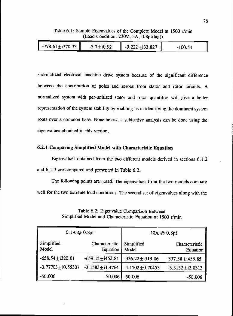
78
Table 6.1: Sample Eigenvalues of the Complete Model at 1500 r/min(Load Condition: 230V, 5A, 0.8pf(lag))
1-778.61±i370.33 ii -5.7±iO.92
H-9.222±i33.827
II
-100.54I
-normalized electrical machine drive system because of the significant difference
between the contribution of poles and zeroes from stator and rotor circuits. A
normalized system with per-unitized stator and rotor quantities will give a better
representation of the system stability by enabling us in identifying the dominant system
roots over a common base. Nonetheless, a subjective analysis can be done using the
eigenvalues obtained in this section.
6.2.1 Comparing Simplified Model with Characteristic Equation
Eigenvalues obtained from the two different models derived in sections 6.1.2
and 6.1.3 are compared and presented in Table 6.2.
The following points are noted: The eigenvaiues from the two models compare
well for the two extreme load conditions. The second set of eigenvalues along with the
Table 6.2: Eigenvalue Comparison BetweenSimplified Model and Characteristic Equation at 1500 r/min
0.1A @ 0.8pf
Simplified CharacteristicModel Equation
1OA 0.8pf
Simplified CharacteristicModel Equation
-658.54±i320.0l -659.15 ±i453.84 -336.22±i3 19.86 -337.58±i453. 85
-3.77703±iO.55307 -3.1583±il.4764 -4.1702±0.70453 -3.3132±i2.0313-50.006 -50.006 -50.006 -50.006

-6.574 -15.21 0.000944 -0.0863 0 0 0.2014
15.21 -6.574 0.0863 0.000944 0 0 0.589
96.56 223.363 -0.049 1.2672 0 0 4.266
-223.363 96.56 -1.2627 -0.049 0 0 -5.4863
0 0 0 0 0 0.0068 0
0 0 0 0 -11.436 -0.551 -285.896
-0.003702 0.001517 -0.0000575 -0.0000081 0.02 -0.000374 -0.00068
(6.18)

real pole of the last eigenvalue are the most dominant poles in the system. The real
eigenvalue can be attributed to the mechanical subsystem because it does not change
with the model simplifications (most of the terms that were neglected during the
simplification process are in the electrical subsystem).
The first set of eigenvalues have frequencies of about 50Hz to 70Hz, closer to
the generator rated frequency and the second set about 0.1Hz to 0.3Hz. Also it is noted
that the first set of poles are damped at a much slower rate than the second set of
poles. The mechanical system is approximately damped at a time constant of about
0.02s.
6.2.2 Changes in Eigenvalues with Load Current
Stability analysis at different load currents is done using the eigenvalues
calculated from the simplified model. The terminal voltage is fixed at 230V and the
load power factor is assumed to be at 0.8(lag). The load current is varied from 1A to
1OA and the corresponding eigenvalues are calculated. Table 6.3 gives the eigenvalues
at different load currents.
It is noted that the real parts of all the eigenvalues are negative, indicating that
the system is stable. The first set of eigenvalues has a natural frequency of about 51Hz
and a damping time constant which increases with increasing load current. The second
set has a much slower damping rate than the first set and a natural frequency variation
of 0.02Hz to 0.12Hz. The real pole corresponding to the mechanical subsystem remains
constant.
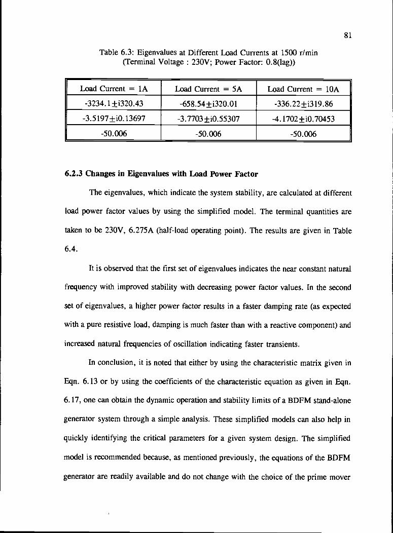
81
Table 6.3: Eigenvalues at Different Load Currents at 1500 r/min(Terminal Voltage: 230V; Power Factor: 0.8(lag))
Load Current = 1A Load Current = 5A Load Current = 1OA
-3234.1 ±i320.43 -658.54 ±i320.01 -336.22 ±i3 19.86
-3.5197±iO. 13697 -3.7703±iO.55307 -4. 1702±iO.70453
-50.006 -50.006 -50.006
6.2.3 Changes in Eigenvalues with Load Power Factor
The eigenvalues, which indicate the system stability, are calculated at different
load power factor values by using the simplified model. The terminal quantities are
taken to be 230V, 6.275A (half-load operating point). The results are given in Table
6.4.
It is observed that the first set of eigenvalues indicates the near constant natural
frequency with improved stability with decreasing power factor values. In the second
set of eigenvalues, a higher power factor results in a faster damping rate (as expected
with a pure resistive load, damping is much faster than with a reactive component) and
increased natural frequencies of oscillation indicating faster transients.
In conclusion, it is noted that either by using the characteristic matrix given in
Eqn. 6.13 or by using the coefficients of the characteristic equation as given in Eqn.
6.17, one can obtain the dynamic operation and stability limits of a BDFM stand-alone
generator system through a simple analysis. These simplified models can also help in
quickly identifying the critical parameters for a given system design. The simplified
model is recommended because, as mentioned previously, the equations of the BDFM
generator are readily available and do not change with the choice of the prime mover
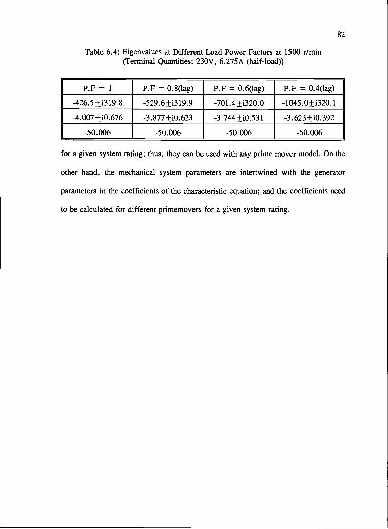
82
Table 6.4: Eigenvalues at Different Load Power Factors at 1500 r/min(Terminal Quantities: 230V, 6.275A (half-load))
P.F = 1 P.F = 0.8(lag) P.F = 0.6(lag) P.F = 0.4(lag)-426.5 ±i319.8 -529.6±i3 19.9 -701 .4±i320.0 -1045.0±i320. 1
-4.007±iO.676 -3.877±iO.623 -3.744±iO.53 1 -3.623 ±iO.392
-50.006 -50.006 -50.006 -50.006
for a given system rating; thus, they can be used with any prime mover model. On the
other hand, the mechanical system parameters are intertwined with the generator
parameters in the coefficients of the characteristic equation; and the coefficients need
to be calculated for different primemovers for a given system rating.

83
Chapter 7
Stand-Alone Generator System- Dynamic Characteristics
After presenting the system characterization and the steady-state characteristics,
this section describes the simulated dynamic characteristics of the BDFM stand-alone
generator system. The BDFM system equations and the 10kW diesel engine along with
a permanent speed-droop governor, as described in Chapter 4, are used in these
studies. All the system results are obtained with the prime mover rated speed at 1500
r/min and with about 5% speed droop for a 2ONm equivalent load.
The generator rated quantities are taken to be 230V and 60Hz. The parameters
of the laboratory prototype machine, as described in Chapter 2, are used. The closed
loop control methods of the generator terminal quantities are designed and studied
taking the IEEE-446 standards from Appendix A as the base values.
The system equations described in Chapter 4 are used in simulating the dynamic
characteristics. In all the simulation runs, the prime mover is assumed to be initially
running at a speed of 1500 r/min.
The frequency regulation in a BDFM stand-alone generator system can be
obtained in two ways:
(1) By tracking the speed signal and adjusting the control excitation
frequency to obtain the rated generator output frequency. Almost all the
prime movers have some kind of speed signal available to their
governors and the same signal can be used for the frequency regulation,
without any additional hardware.
(2) By directly sensing the generator output frequency using a frequency-to-
voltage converter (FTVC). The problem with it is that the response
times of the FTVC are very long for low frequency signals and the
dynamic response based on this signal will not be satisfactory.
It was decided to use the first method for frequency regulation.
7.1 Open Loop Characteristics
The simulated results of the system under open loop condition (with no control
of the terminal quantities) are presented. The control excitation is initially set at a
current excitation of 2.6A, corresponding to the generator terminal voltage of 230V;
and at a frequency of 40Hz, which when combined with the shaft speed of 1500r/min
will result in a generator terminal frequency of 60Hz. The load is represented in terms
of resistive values, with higher load resistance resulting in lower load current and vice
versa. A nominal resistive load of 50011 is set at the generator terminals (true open
circuit is difficult to simulate).
Figure 7.1 shows the system open loop results under start-up and sudden load
conditions. At start-up, the prime mover rotational speed is assumed to be 1500r/min.
The system results are obtained from t = 0.0 is. It can be noted that the terminal
voltage reaches 230V after the initial oscillations. The terminal frequency drops down
to about 59.75Hz due to the slight drop in the prime mover speed caused by the
nominal load (0.25A load current) assumed at start-up.
Figures 7.1(c) and 7.1(d) show the terminal quantities after a sudden electrical
load change (terminal load resistance changed from 50012 to 5012, thus increasing the
load current) applied at t = 1.5 is. it is observed that the terminal quantities further

85
300
250
200
150
100
50
0-Il-
0.0
61.0
60.5
0
60.0
59.5
59.0-I-
0.0
0.3 0.6 0.9 1.2 1.5
Thne (s)
0.3 0.6 0.9 1.2 1.5
Thie (s)
(b)
Fig. 7.1. Open Loop Characteristics Under Start-up

250
225
200
175
150
125
100-1-1.5
60.0
59.5
0
59.0
58.5
58.0-4--
1.5
1.8 2.1 2.4 2.7 3.0
Thne (s)
(c)
1.8 2.1 2.4 2.7 3.0
me (s)
(d)
Fig. 7.1. Open Loop Characteristics Under Load

87
reduce, away from the rated quantities. The terminal voltage decreases to 170V and the
frequency to 58.75Hz.
These base values obtained through the open-loop studies indicate the system
dynamics with no controller on the generator. The following sections describe the
results of closed loop control methods applied for stand-alone system regulation.
Conventional proportional-integral method as well as modern fuzzy control methods are
used in arriving at the results.
7.2 Closed Loop System Regulation using P1 Control
7.2.1 Closed Loop Voltage Regulation Alone
The rationale behind presenting the results of this subsection is to show the
analogy with conventional, synchronous-machine based, stand-alone generators. In the
conventional systems with speed-droop governors and synchronous generators, only the
voltage regulation is implemented and the terminal frequency is left alone (frequency
changes with the prime mover speed droop). Similar conditions were simulated with
the BDFM stand-alone generator system.
Figure 7.2 gives the PT control scheme in block diagram form. The PT gains
used are: 0.5 and 0.1 for the voltage-regulation; and 0.1 and 0.01 for the frequency-
regulation.
Figure 7.3 shows the start-up transients and Fig. 7.4 gives the sudden load
transients of the effects of the voltage regulation using a simple P1 control scheme. In
both the cases, the terminal voltage settles at the rated value of 230V and the excitation

2*lt
fc
i2*3Voltage Regulation
\ + vdp"2
- *
230V '_________ Ic BDFM System Eqns.I_____ (Eqns.4.6and47)
andDiesel System Eqns.
*
P1fc (Eqn. 68)
Frequen' Reation
Fig. 7.2. P1 Control Scheme in Block Diagram Form
(Or
current changes to control the terminal voltage. The terminal voltage is calculated using
the d-q axes quantities as shown below:
Vtcri = I- * 2 + V 2'dp qp/
(7.1)
Figure 7.5 shows the changes in the frequency when voltage regulation alone
is considered. The frequency drops to 59.75Hz from an initial value of 60Hz for a near
open circuit condition and further drops to about 57.7Hz after a sudden load change.
Most of the electronic-equipment loads operate with narrow input frequency limits,
combined with strict limits on the volt-time rating. This makes the response of the
system with voltage regulation alone unacceptable in many applications. This is the
reason the advanced, electronic governors are designed and used with most of the
prime movers to achieve the 'isochronous' operation, maintaining the rated terminal

300
250
200
C150
100
6
CS.)
U
1II
04L
0.0
01L0.0
0.3 0.6 0.9 1.2 1.5
Thue (s)
(a)
0.3 0.6 0.9 1.2 1.5
Time (s)
(b)
Fig. 7.3. Start-up Transients with Voltage Regulation Alone (PT Control)

250
225
4)
4-,
C4)4)C.)
200
175+-1.5
6
0+-1.5
1.8 2.1 2.4 2.7 3.0
Time (s)
(a)
1.8 2.1 2.4 2.7 3.0
Time (s)
(b)
Fig. 7.4. Transients Under Load with Voltage Regulation Alone (P1 Control)
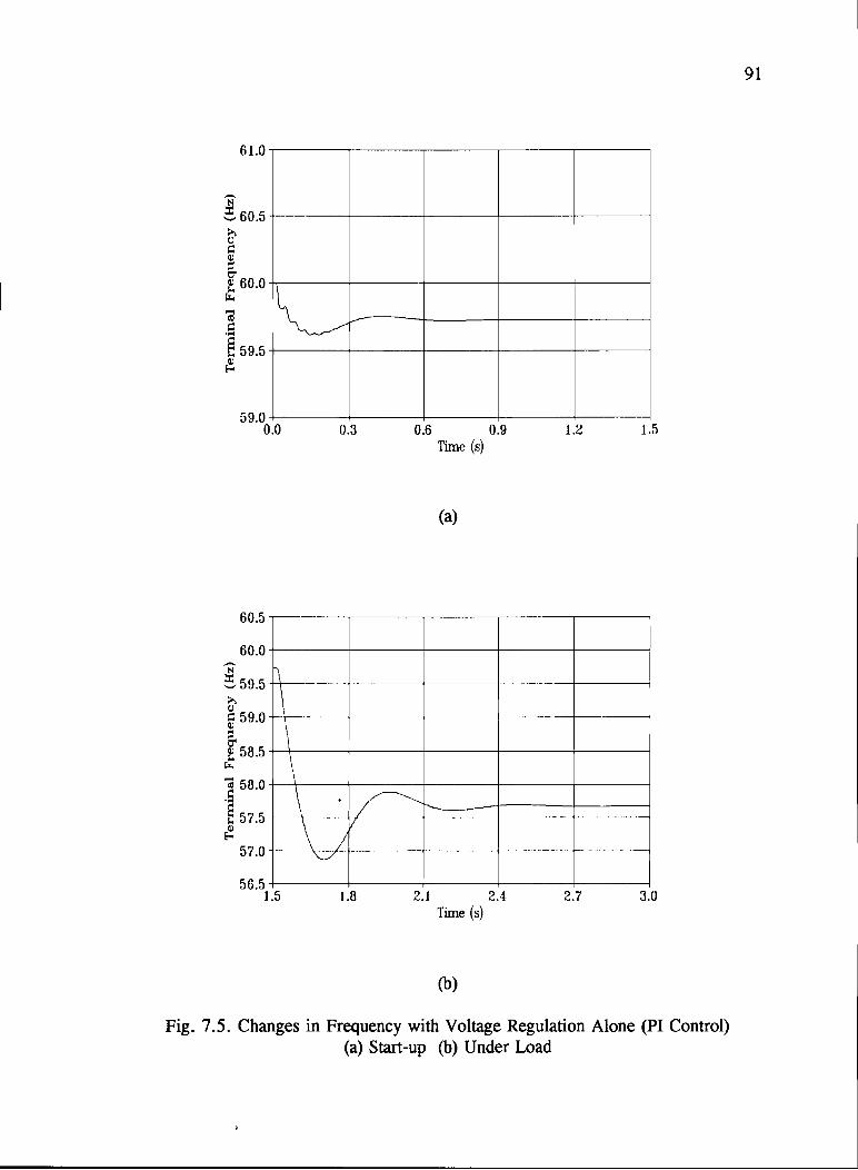
91
61.0
60.5
C)
60.0
59.5
59.0-i-0.0
60.5
60.0
,59.5
59.0
58.5
58.0
57.5
57.0
56.5+-1.5
0.3 0.6 0.9 1.2 1.5
The (s)
(a)
1.8 2.! 2.4 2.7 3.0
Time (s)
(b)
Fig. 7.5. Changes in Frequency with Voltage Regulation Alone (P1 Control)(a) Start-up (b) Under Load

frequency. The one major advantage of using the BDFM generator system is that even
with simple, speed-droop governors, terminal frequency regulation can be achieved by
controlling the excitation frequency. This novel aspect of the BDFM generator is the
focus of the next section.
7.2.2 Closed Loop Voltage and Frequency Regulation
A conventional P1 control method is used for the terminal voltage and frequency
regulation. Figs. 7.6 to 7.8 show the start-up transients under closed loop control with
the control applied at t = 0.0 is. Fig. 7.7 shows the transients of frequency response.
The control winding frequency tracks the droop in speed (Eqn. i. i) to maintain a
constant generator terminal frequency at 60Hz after the initial transients. The terminal
voltage reaches the rated steady state reference value in about 0.4s and the terminal
frequency in 0.6s. Fig. 7.8 shows the generator power winding Q-axis and A-phase
currents, respectively. It is observed that the Q-axis current has a frequency equal to
the synchronous frequency and that the A-phase current has a frequency value of 60Hz.
The load current resulting from the nominal load resistance is 0.25A.
A sudden load change is applied at t 1.5 is, by changing the load resistance
from 5000 to 500. Figs. 7.9 to 7.11 show the system voltage and frequency transients.
The voltage momentarily dips to 1 80V (about 21 % under-voltage) and after some
oscillations, settles back at the rated value. During this process, the power demand is
first delivered by the prime mover inertial system as well as the increase in control
winding excitation, before the prime mover slows down as per Fig. 4.3 to deliver more
power. The changes in control excitation during this voltage regulation can be noted
in Fig. 7.9(b). As expected, the required control excitation increases with the increased
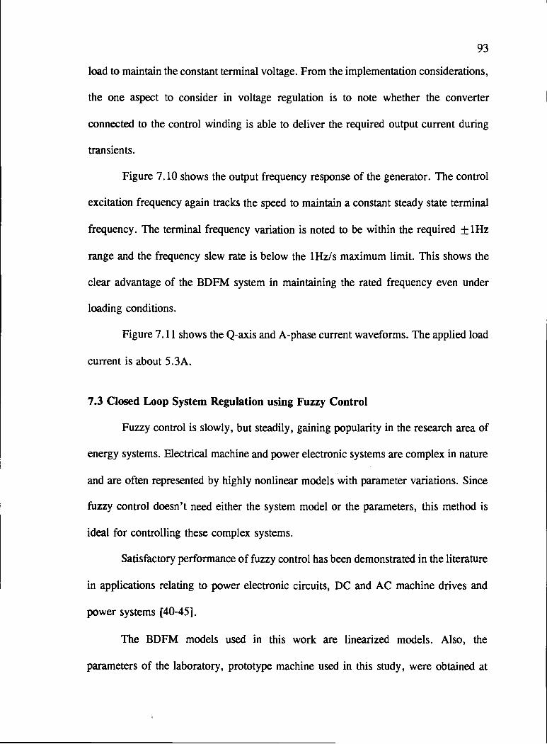
93
load to maintain the constant terminal voltage. From the implementation considerations,
the one aspect to consider in voltage regulation is to note whether the converter
connected to the control winding is able to deliver the required output current during
transients.
Figure 7.10 shows the output frequency response of the generator. The control
excitation frequency again tracks the speed to maintain a constant steady state terminal
frequency. The terminal frequency variation is noted to be within the required ±1Hz
range and the frequency slew rate is below the 1Hz/s maximum limit. This shows the
clear advantage of the BDFM system in maintaining the rated frequency even under
loading conditions.
Figure 7.11 shows the Q-axis and A-phase current waveforms. The applied load
current is about 5.3A.
7.3 Closed Loop System Regulation using Fuzzy Control
Fuzzy control is slowly, but steadily, gaining popularity in the research area of
energy systems. Electrical machine and power electronic systems are complex in nature
and are often represented by highly nonlinear models with parameter variations. Since
fuzzy control doesn't need either the system model or the parameters, this method is
ideal for controlling these complex systems.
Satisfactory performance of fuzzy control has been demonstrated in the literature
in applications relating to power electronic circuits, DC and AC machine drives and
power systems [40-45].
The BDFM models used in this work are linearized models. Also, the
parameters of the laboratory, prototype machine used in this study, were obtained at
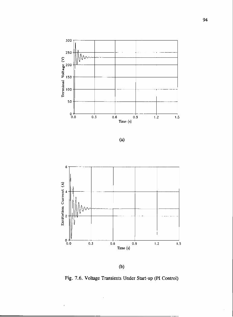
300
250
200
0150
100
50
C)
C
C)
04'-0.0
6
0-1'-
0.0
0.3 0.6 0.9 1.2 1.5
Tüe (s)
(a)
0.3 0.6 0.9 1.2 1.5
Thiie (s)
(b)
Fig. 7.6. Voltage Transients Under Start-up (P1 Control)
94

60.25
60.15
C)
60.05
59.95
E59.85
59.75+-0.0
40.5
40.0
03.s
39.0 +-0.0
0.3 0.6 0.9 1.2 1.5
Thue (s)
(a)
0.3 0.6 0.9 1.2 1.5
Time (s)
(b)
Fig. 7.7. Frequency Transients Under Start-up (PT Control)
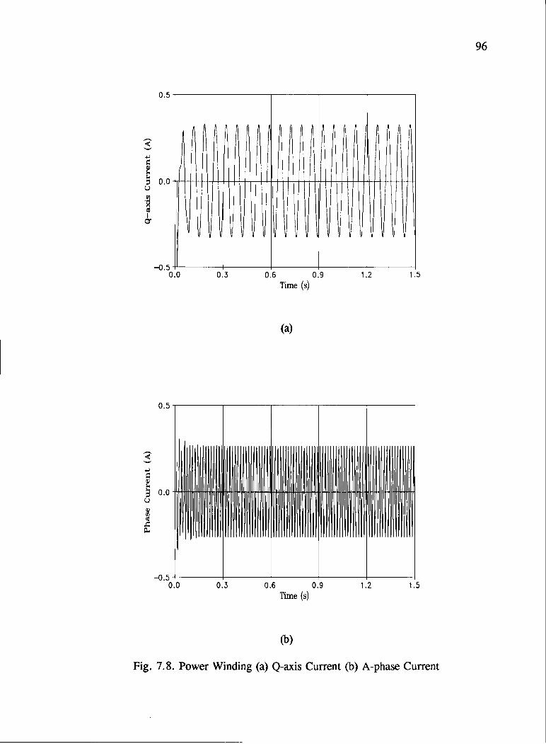
0.5
0.00
-0.50.0
0.5
0.00
-0.50.0
0.3 0.6 0.9 1.2 1.5
The (s)
(a)
0.3 0.6 0.9 1.2 1.5
Thne (s)
(b)
Fig. 7.8. Power Winding (a) Q-axis Current (b) A-phase Current

97
300
275
a)
250
225
200
175+-1.5
6
4-,
04-)
C)40
2 +-1.5
1.8 2.1 2.4 2.7 3.0
Time (s)
(a)
1.8 2.1 2.4 2.7 3.0
Time (s)
(b)
Fig. 7.9. Voltage Transients Under Load (PT Control)

60.5
N
60.0
0)
C.0)
. 59.5
0)
59.0+-1.5
40.0
39.5N
39.00
0)
38.5
38.0
0
37.0
36.5 +-1.5
1.8 2.1 2.4 2.7 3.0
Thne (s)
(a)
1.8 2.1 2.4 2.7 3.0
Time (s)
(b)
Fig. 7.10. Frequency Transients Under Load (P1 Control)
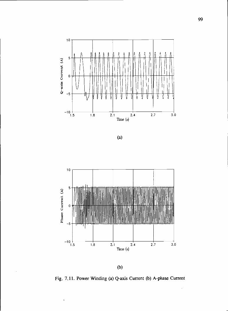
ii'
4.)
0U
-10 -f-1.5
10
'-5
0U
-5
-10 -i---
1.5
1.8 2.1 2.4 2.7 3.0
Tune (s)
(a)
1.8 2.1 2.4 2.7 3.0
Time (s)
(b)
Fig. 7.11. Power Winding (a) Q-axis Current (b) A-phase Current

two operating points in the low-speed region and may not be completely true in the
high-speed region. This is an ideal situation for considering the fuzzy control method.
The fuzzy control method is applied to the BDFM, stand-alone generator system
control, and the results are presented in this section.
Appendix B gives a brief introduction to the theory of fuzzy control.
Eventhough, equivalent PD-like and PID-like fuzzy control schemes are also feasible,
a P1-like control scheme is considered in this section to enable comparison with the
results of the previous section. A fuzzy control implementation of the conventional PT
control is given in Appendix B. The calculation of the change in control variable (du)
based on the information of output error (e) and change in output error (de) is
considered equivalent to implementing a conventional PT control scheme. The
equivalent integration in the fuzzy control scheme is provided by the change in the
control variable, which is due to the accumulation of the error in the corresponding
output variable (such as in the conventional P1 control) and thus, can be positive or
negative depending on the signs of the output error and change in output error.
While designing a fuzzy controller, the following points need to be noted:
(1) in a fuzzy logic controller, the number of primary fuzzy sets determine the
granularity of the control; (2) the number of quantization levels should be large enough
to provide an adequate approximation and yet be small to save memory storage; (3)
most often, the fuzzy sets are uniform in resolution, but coarse resolution can be used
for large errors and fine resolution for small errors to obtain a better control as well
as to obtain as small a steady state error as possible; (4) if the measurable data is noise
101
prone, the membership functions should be chosen as wide as possible. Membership
functions can be of any shape which can be mathematically analyzed.
Figure 7.12 shows the membership functions of the fuzzy variables for the
generator terminal voltage regulation. The input variables are the error in voltage (ev)
from the set point of 230V and the change in error (cev). The output variable which
represents the change in control excitation current is shown as di2.
A triangular fuzzy membership function is chosen in this study along with a
50% overlap between the membership functions. This gives only two fuzzy rules per
input variable, resulting in a total of four fuzzy rules per operating point. The chosen
quantization levels are 5V for error in voltage, 0.5V for change in error and 0. 1A for
the change in control effort. There are 9 membership functions for each input variable
and 11 for the output variable. The fuzzy sets are linguistically represented as NVB
(negative very big), NB (negative big), NM (negative medium), NS (negative small),
Z (zero), PS (positive small), PM (positive medium), PB (positive big) and PVB
(positive very big).
Table 7.1 gives the rule base for calculating the change in control excitation
based on the terminal voltage error. The output is selected as follows:
Suppose the error in terminal voltage is 7V and the change in error is -1 .2V.
From the input membership functions, we gather that the two fuzzy sets, PS and
PM corresponding to voltage error, and the two fuzzy sets, NM and NB
corresponding to the change in error will be activated. The degree of
membership (weighage) is calculated for each of these four sets by solving for
the equation of a straight line where the straight lines are the part of the
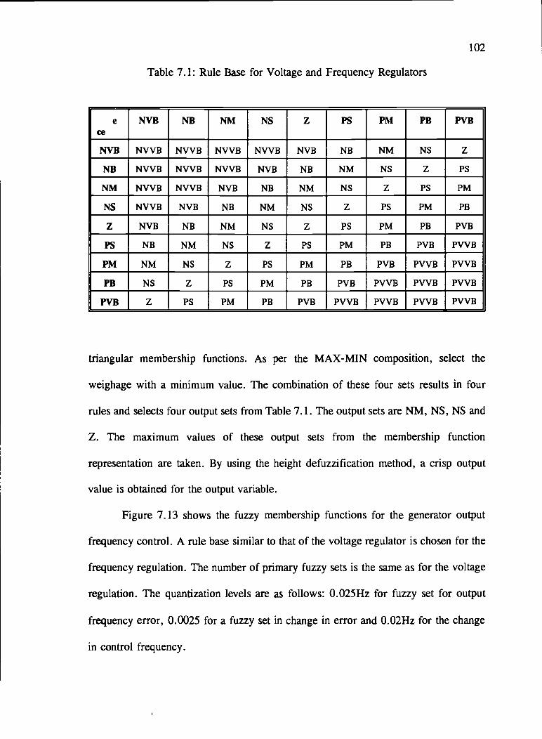
102
Table 7.1: Rule Base for Voltage and Frequency Regulators
ceNVB NB NM NS Z PS PM PB PVB
NVB NVVB NVVB NVVB NVVB NVB NB NM NS Z
NB NVVB NVVB NVVB NVB NB NM NS Z PS
NM NVVB NVVB NVB NB NM NS Z Ps PM
NS NVVB NVB NB NM NS Z Ps PM PB
Z NVB NB NM NS Z PS PM PB PVB
PS NB NM NS Z PS PM PB PVB PVVB
PM NM NS Z PS PM PB PVB PVVB PVVB
PB NS Z PS PM PB PVB PVVB PVVB PVVB
PVB Z PS PM PB PVB PVVB PVVB PVVB PVVB
triangular membership functions. As per the MAX-MIN composition, select the
weighage with a minimum value. The combination of these four sets results in four
rules and selects four output sets from Table 7.1. The output sets are NM, NS, NS and
Z. The maximum values of these output sets from the membership function
representation are taken. By using the height defuzzification method, a crisp output
value is obtained for the output variable.
Figure 7.13 shows the fuzzy membership functions for the generator output
frequency control. A rule base similar to that of the voltage regulator is chosen for the
frequency regulation. The number of primary fuzzy sets is the same as for the voltage
regulation. The quantization levels are as follows: 0.025Hz for fuzzy set for output
frequency error, 0.0025 for a fuzzy set in change in error and 0.02Hz for the change
in control frequency.
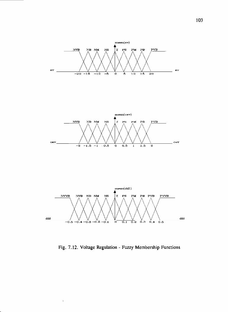
ev
oev
103
rnern(ev)
20 15 10 5 0 5 10 15 20
nierr(cev)
2 1.5 1 0.5 0 05 1 1.5 2
mem(di2)
NVVB NVB NB NM NS TZ PS PM PB PVB PVVI3
UI- yyyyryyyy
ev
cev
Fig. 7.12. Voltage Regulation Fuzzy Membership Functions

mem(ef)
ef ef0.075 0.025 0 0.025 0.075
0.1 0.05 0.05 0.1
cef
dt2
mem( cef)
0.01 0.005 0 0.005 0.010.0075 0.0025 0.0025 0.0075
mem(df2)
NVVB NVB NB NM NS I Z PS PM PB PVB PVVB
0.1 0.06 0.02 0 0.02 0.06 0.10.08 0.04 0.04 0.08
cef
r.r
Fig. 7.13. Frequency Regulation Fuzzy Membership Functions
104

105
The dynamic responses of the stand-alone system using closed-loop fuzzy
control are obtained under similar conditions as used with the closed-loop PT control
in the previous section. Fig. 7.14 shows the start-up response of the generator terminal
voltage. The response has less overshoot as well as a faster settling time than the case
with the P1 control. It is noted that this response is possible due to the fuzzy control
method exerting more control effort for a larger error in the controllable quantity. This
can be seen in the response of the control excitation current which has a large value
initially in bringing the terminal voltage towards the set point faster. However, in
reality, the system response will be dictated by either a current-limiter or the dv/dt
capability of the converter switches, both of which can limit the control current
excitation. Fig. 7.15 shows the output frequency response and it is noted that the
frequency almost stays constant with the control frequency tracking the system speed
changes.
The generator output response for a sudden load change, with load resistance
decreased from 500t) to 5011, is shown in Figs. 7.16 and 7.17. It can again be observed
that the responses are superior to those of the previous section using the PT control. It
should be noted that while obtaining the responses, the P1 parameters were tuned to
obtain best responses in the previous section, but no such tuning was done while testing
the fuzzy control method. This indicates the fact that implementing a fuzzy control
algorithm is much easier than using a conventional method.
Fig. 7.18 shows an interesting result pertaining to the stability of the system.
The figure shows the membership functions selected by the algorithm under the start-up
condition. In these figures, 0 corresponds to the membership set NVB and 8
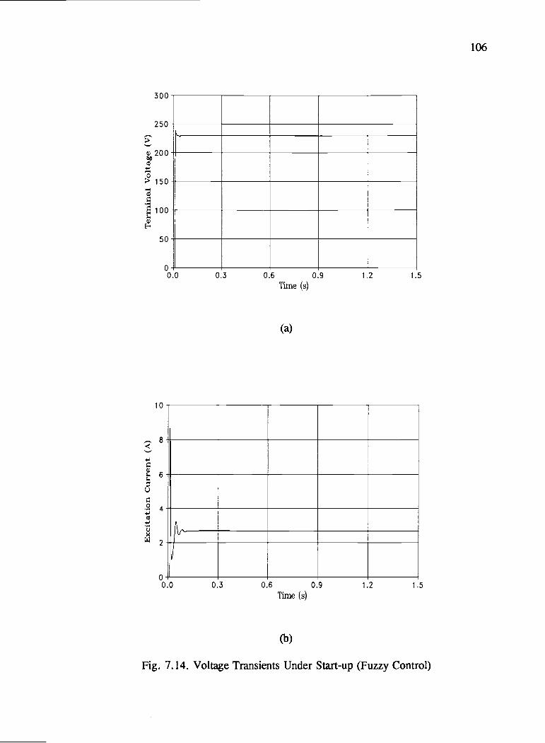
300
250
200
150
100
50
0-I'-
0.0
L)
0
0-Il--
0.0
0.3 0.6 0.9 1.2 1.5
Thne (s)
(a)
0.3 0.6 0.9 1.2 1.5
Time (s)
(b)
Fig. 7.14. Voltage Transients Under Start-up (Fuzzy Control)

60.3
60.1
V
a)
059.9
59.7 +-0.0
40.5
40.0a)
039.5
39.0 +-0.0
0.3 0.6 0.9 1.2 1.5
Time (s)
(a)
0.3 0.6 0.9 1.2 1.5
Time (s)
(b)
Fig. 7.15. Frequency Transients Under Start-up (Fuzzy Control)

108
250
225
200
175+-1.5
8
L)4
0
Q
0+-1.5
1.8 2.1 2.4 2.7 3.0
Time (s)
(a)
1.8 2.1 2.4 2.7 3.0
Time (s)
(b)
Fig. 7.16. Voltage Transients Under Load (Fuzzy Control)

60.5
60.2
C)
59.9
59.6
I..
59.0+-1.5
40
39
038
C)
37+-1.5
1.8 2.1 2.4 2.7 3.0
Thne (s)
(a)
1.8 2.1 2.4 2.7 3.0
Time (s)
(b)
Fig. 7.17. Frequency Transients Under Load (Fuzzy Control)
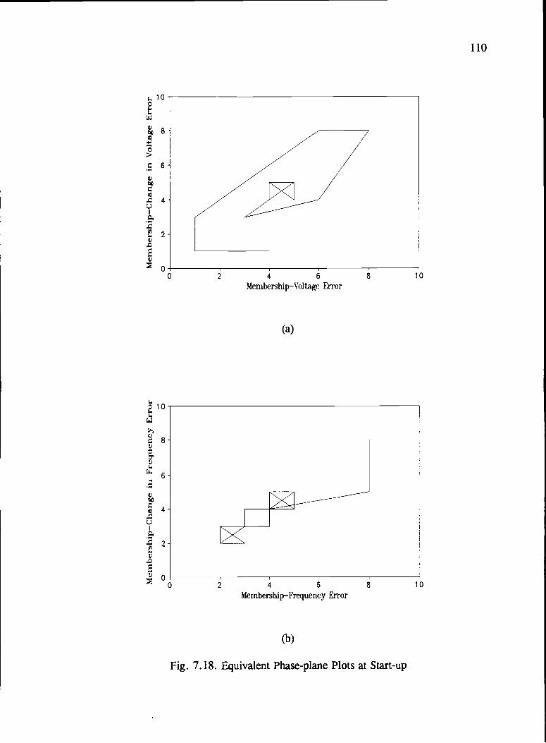
100
0
0
10
0
0
0
E
0 2 4 6 8 10
Membership-Voltage Error
(a)
ol0 2 4 6 8 10
Membership-Frequency Error
(b)
Fig. 7.18. Equivalent Phase-plane Plots at Start-up
110
111
corresponds to the membership set PVB. The trajectory shows the membership of
"change in error" plotted against the membership of "error". It can be observed that
the plot settles about the membership function 5, indicating that the error as well as the
change in error have reached zero or oscillating about zero. The result of these
oscillations can be noted in the responses presented earlier, indicating the fact that a
direct fuzzy control alone cannot guarantee a zero steady state error. This is a
limitation of the direct fuzzy control. The remedy for this problem is to choose finer
fuzzy sets about the zero membership set. Alternatively, a P1 method can be used along
with the fuzzy scheme, whereby a fuzzy algorithm is used for larger errors and a P1
loop can be activated near the set point. This is called "hybrid fuzzy-PI" (nearby-
faraway) control.
Also, from the Fig. 7.18, it can be seen how certain areas of the quantization
do not relate to the system trajectory. From the design point of view, this trajectory
provides interesting guidelines for the system analysis. One can easily modify the rules
that are not selected in this trajectory. Although most of the discussion above is
qualitative, it is enough to characterize the dynamic behavior of the fuzzy feedback
system.
7.4 System Responses to Small Load Changes
In the previous section, it was concluded that a direct fuzzy control alone cannot
result in a zero steady state error of the controllable quantity. A PT loop can be added
to achieve the required steady state value. Simulation results are obtained as to how the
fuzzy control compares with a conventional control if very small load changes occur
at regular, short intervals. A simulated load, as shown in Fig. 7.19, is applied to the
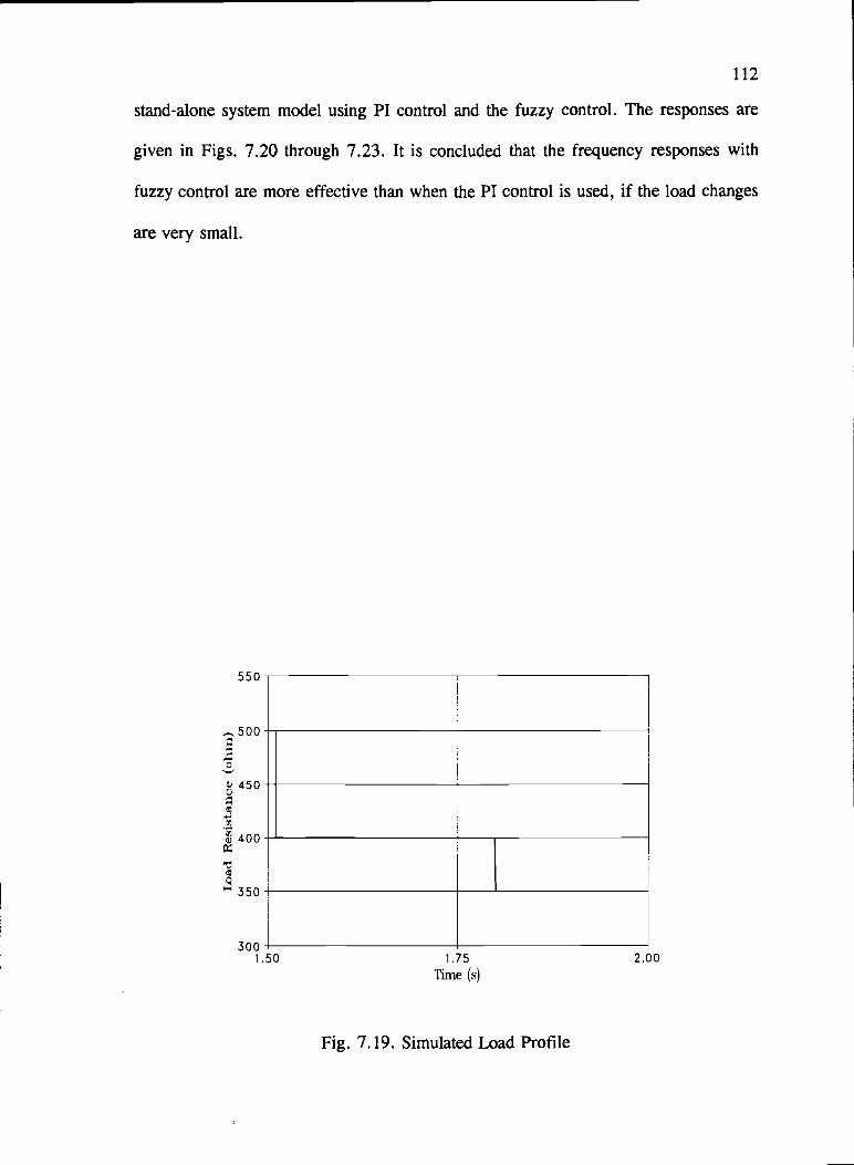
112
stand-alone system model using P1 control and the fuzzy control. The responses are
given in Figs. 7.20 through 7.23. It is concluded that the frequency responses with
fuzzy control are more effective than when the P1 control is used, if the load changes
are very small.
550
500
0
450
400
350
300 +-1.50 1.75
Thne (s)
Fig. 7.19. Simulated Load Profile
2.00

113
0
C)
300
250
200 +-1.50
1+-1.50
1.75 2.00Time (s)
(a)
1.75 2.00
Time (s)
(b)
Fig. 7.20. Voltage Transients for Small Load Disturbances (PT Control)

114
60.2
N
60.1
41
60.0
C)
0
C)N
59.9 +-1.50
40.00
39.75
39.50
1.75 2.00
Time (s)
(a)
50 1.75 2.00
Time (s)
(b)
Fig. 7.21. Frequency Transients for Small Load Disturbances (PT Control)
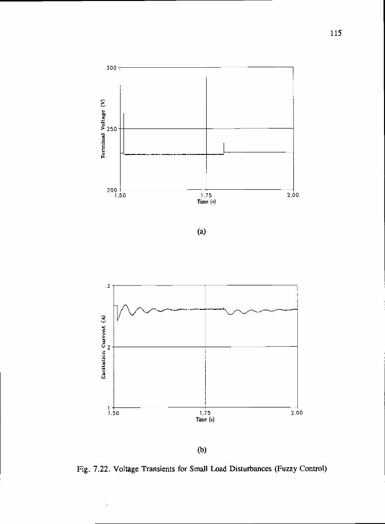
115
300
250
200
V
0*.,
C)
x
H-1.50
50 1.75 2.00
Time (s)
(a)
1.75 2.00
me (s)
(b)
Fig. 7.22. Voltage Transients for Small Load Disturbances (Fuzzy Control)

116
60.15
60.05
V
g59.95
59.85
0
0
C)
59.75 -I---
1.50
40.00
39.75
39.50 +-1.50
1.75 2.001me (s)
(a)
1.75 2.00Time (s)
(b)
Fig. 7.23. Frequency Regulation for Small Load Disturbances (Fuzzy Control)
117
Chapter 8
Experimental Results
Previous chapters have introduced the BDFM as a stand-alone generator system
and the feasibility and characteristics are discussed with a diesel engine as the prime
mover. Using simulation studies, it was shown that the dynamic responses of a stand-
alone system based on a BDFM generator are satisfactory. This chapter presents some
experimental results obtained by using the laboratory prototype machine, which was
described in Chapter 2. The idea behind this exercise is to show the feasibility of a
BDFM stand-alone generator system in the laboratory. It was mentioned in Chapter 5
that the rated terminal voltage of 230V is not obtainable using the prototype machine
because of limitations of the laboratory converter as well as the saturation of the BDFM
control winding above low current levels. The tests are conducted assuming the
generator rated quantities to be 1 iSV, 60Hz. Both the terminal voltage and the terminal
frequency of the generator are regulated.
8.1 Experimental Setup
Figure 8.1 shows the experimental system in block diagram form. The details
of all the major components are described below:
8.1.1 Prime Mover
It was previously mentioned that this study would prove that a diesel engine
even with a governor having speed-droop characteristics is enough for a BDFM stand-
alone system. The results presented in Chapter 7 show that indeed is the case. Instead
of a diesel engine, a commercially available, four-quadrant, 15kW DC drive is used

118
PowerEEEs_Transducer /
ControlWinding
PowerConverter
i*$ 4F*
SignalConversionCircuitry
80196Eval Board
Controller
VoltageTransducer(rms)
Fig. 8.1. Experimental Setup - Block Diagram
as the prime mover. It is well known that a shunt connected DC machine has a natural
speed droop characteristics under increasing load torque. The tests on the DC drive
have shown that for a constant armature voltage setting, the DC drive has a speed
droop of 4 percent for 3kW (20% of the rated DC drive load), at a speed of 1500
r/min. Thus the DC drive with a fixed armature voltage setting is used to drive the
laboratory BDFM.
8.1.2 Generator
The laboratory prototype BDFM having a 6/2 stator pole combination is used.
The rated synchronous speed of this machine is 900 r/min and in this study, to maintain
consistency with the theoretical study, the rated operating speed is taken to be 1500
119
rimin. It should be noted that from the conclusions from Chapter 5, this machine is
best operated slightly above a speed of 900 r/min.
8.1.3 Power Converter
An experimental, 15kVA Series Resonant Converter (SRC) with a maximum
output voltage limit of 240V is connected to the control winding terminals in this study.
This converter can be operated manually as well as remotely. Remote operation in the
current-control mode is chosen for the experiments. The converter accepts analog
signals as commands for setting the output current and frequency. During the
experiments, the converter is connected to the power grid where as in a practical stand-
alone system, the input power is supplied from the generator output (power winding
terminals).
8.1.4 Load
Water rheostat boxes, connected in parallel, are used as load to the power
winding terminals; so the test results presented in this chapter are based on unity power
factor loads. From the point of dynamics, pure resistance loads create worst case
system transients due to the absence of reactance elements; so, the experimental results
should give a good indication of BDFM stand-alone system operation.
8.1.5 Controller
An 80196 microcontroller based [46-48] control is designed to implement the
control algorithm. The details of the controller design and hardware implementation is
the focus of the next section.
120
8.2 Controller Design and Implementation
Voltage regulation is implemented by directly sensing the rms terminal voltage
using an rms transducer (bandwidth of dc to 5kHz) and adjusting the control current
accordingly. The frequency regulation, as discussed earlier, can be accomplished either
by direct sensing of the generator frequency or by sensing the speed signal and then
commanding the appropriate control frequency to obtain the rated generator frequency.
Speed sensing is used in the experiments.
The hardware design utilizes the built-in Analog-to-Digital Conversion (ADC)
and High-Speed-Output (HSO) modules in the 80196 microcontroller. While the ADC
module has 10-bit resolution, the HSO module can be used in implementing a highly
accurate 8-bit digital-to-analog conversion. Two of the channels in the ADC module
are used in sensing the terminal voltage and speed signals. Two of the pins in the HSO
Module are used in commanding the required converter output.
The fuzzy control algorithm, as discussed in Chapter 7 is implemented with
proper scaling to suit the 1 15V operation. A fixed-point microprocessor like the 80196
(or even an 8-bit processor) is enough to implement this algorithm.
Upon the start-up of the system, the ADC module starts sensing the terminal
voltage signal from the rms voltage transducer and the speed signal from a shaft-
mounted speed transducer. In the control algorithm, the microcontroller outputs the
resultant control commands in the form of a rectangular pulse train that varies in duty
cycle with a fixed period. The pulse trains from the HSO pins dictate the average value
of the analog command, that needs to be supplied to the power converter, to obtain the
appropriate waveform at the control winding terminals.

121
Figure 8.2 shows the signal conversion circuit. A buffer is used to make the
command output swing rail to rail. A low pass filter (cut-off frequency of 1Hz) in the
form of a simple R-C circuit (1.5k(, 100.tF) is used to obtain a smooth analog signal
from the pulse train. Operational amplifier circuits with appropriate gains are used to
provide the analog commands to the power converter. The power converter accepts the
analog signals in the range of 0-5V or 0-bY. A O-1OV range is used for better
resolution.
An 80196 microcontroller evaluation board [49] is used to implement the
algorithm.
8.3 Experimental Results
The tests are performed about a nominal speed of 1500 r/min. Initially the DC
machine alone is started and run at a speed of 1500 r/min and the armature voltage
80196
Pulse Train1150 Pin
Buffer 1.owpass AmplifierFilter
Analog0utpu1
Fig. 8.2. Pulse to Analog Signal Conversion Circuitry

122
setting is fixed for the rest of the experiments. This condition simulates the prime
mover running at the rated speed in a stand-alone generator system with a speed-droop
governor. Then, a command for start-up is supplied to the BDFM generator controller
with open-circuited power winding terminals. This test condition is similar to the start-
up condition used in the simulation studies.
Figure 8.3(a) shows the transient responses of the rms quantities of the terminal
voltage and control currents. Initially the terminal voltage is zero and upon start-up,
the voltage ramps up with the increasing control current. The initial steep increase in
control current is in line with the fuzzy algorithm philosophy of larger correction for
larger errors. The control current quickly ramps up to about l7A before dropping back
to its steady state value of 4.2A. The maximum value of control current is designed in
order not to trip the over-voltage relay in the converter. After a quick ramp, the
terminal voltage settles at 1 15V in about 350ms. One drawback that was noted is that
the resolution in converter current control is in steps of O.3A (at an internal update rate
of about 3Oms) which results in significant changes in the generator terminal voltage
even for a one step change in control current. But it can be observed that the terminal
voltage is reasonably well settled. Fig. 8.3(b) gives the instantaneous responses of the
generator voltage and control current quantities. The steep change in control current
at the time of start-up can be observed. Also, initially the control winding rotational
frequency is lower than the rotational speed of the prime mover. This results in control
winding generating power and thus, the initial negative current thatcan be observed in
Fig. 8.3(b).

123
/p .t000ed
-.00000 L50000 4.00000 ;
I ,t
Fig. 8.3(a). Transient Responses of Voltage Regulation at Start-up (RMS Values)(Top Trace: Terminal Voltage 150 V/div)(Bottom Trace: Control Current 10 A/div)
#p topcied
-eo,0000 p20,000 1.9200020C' tidiv
Fig. 8.3(b). Transient Responses of Voltage Regulation at Start-up (Inst. Values)(Top Trace: Terminal Voltage 100 V/div)(Bottom Trace: Control Current 20 A/div)

124
Figure 8.4 shows the speed and control frequency responses. Upon start-up, the
control frequency increases to 40Hz resulting in a 60Hz terminal voltage waveform and
starts tracking the speed. Meanwhile, the speed drops down temporarily under the
initial generating torque applied from the control winding, before regaining its no-load
value. The high value of torque as well as the speed change can be attributed to the
control current magnitude at startup, which indicates that the membership functions at
the extremes need to be modified.
Figure 8.5 gives the resultant terminal voltage waveform under no-load
conditions. One can observe the effect of the slot harmonics in the waveform. These
slot harmonics can be observed even when the power winding is supplied from the
/p .topped
- .00000 1.50000 4,00000 ;
500 /iii
Fig. 8.4. Transient Responses of Frequency Regulation at Start-up(Top Trace: Speed 80 r/min/div)
(Bottom Trace: Control Frequency Command 18 Hz/div)
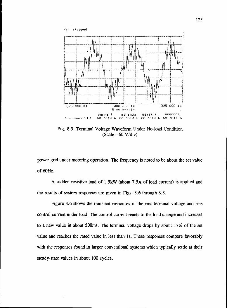
125
/p stopped
675.000 rn 900.000 rn 925.000 m5.00 Jdiv
current minimum me,imum overagefroni,oriru( I 'f 14 I4 P(iIJ14 F4, 0.3614 b 60.3614 H
Fig. 8.5. Terminal Voltage Waveform Under No-load Condition(Scale 60 V/div)
power grid under motoring operation. The frequency is noted to be about the set value
of 60Hz.
A sudden resistive load of 1.5kW (about 7.5A of load current) is applied and
the results of system responses are given in Figs. 8.6 through 8.8.
Figure 8.6 shows the transient responses of the rms terminal voltage and rms
control current under load. The control current reacts to the load change and increases
to a new value in about 500ms. The terminal voltage drops by about 17% of the set
value and reaches the rated value in less than is. These responses compare favorably
with the responses found in larger conventional systems which typically settle at their
steady-state values in about 100 cycles.
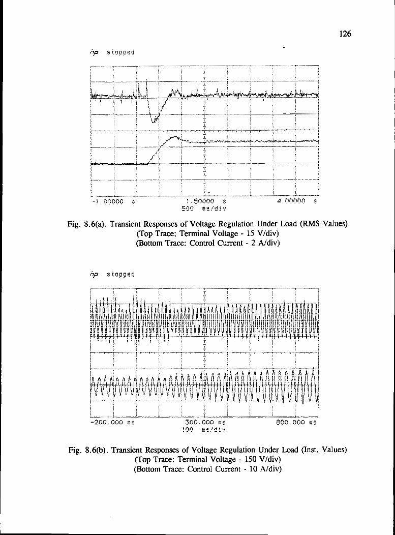
fp s.oppe']
126
1.500OC) 4.00000,,.I *
Fig. 8.6(a). Transient Responses of Voltage Regulation Under Load (RMS Values)(Top Trace: Terminal Voltage - 15 V/div)(Bottom Trace: Control Current 2 A/div)
ip stc'ppd
r' , A IY fi f fl UJ i') J H f. S1.! R..... ,....t ...............
2flfl.flOU OO.00fl i ROO.()C)O uc
M. 1,44(1
Fig. 8.6(b). Transient Responses of Voltage Regulation Under Load (Inst. Values)(Top Trace: Terminal Voltage - 150 V/div)(Bottom Trace: Control Current 10 A/div)

127
Figure 8.7 shows the drop in speed with application of a sudden load and the
control frequency follows almost instantaneously. The speed drops by about 60 r/min
and it is noted that the frequency regulation is attained in about is. The waveforms of
the generator terminal quantities(V and Ib) are given in Fig. 8.8 and it can be
observed that the frequency of these sinusoidal waveforms is about 60Hz.
This work uses the responses of the system speed and control frequencies in
arriving at the generator output frequency. Integrated circuits like the AD650 (FTVC)
can be used in sensing or measuring the terminal frequency. In a system where speed
signals are already available, this cost can be avoided. Otherwise, the F-to-V
conversion ICs can be used to sense the output frequency for the frequency regulation,
except that these ICs are prohibitively expensive. A digital method of measuring the
pulse widths based on the generator voltage waveform zero crossing and thus adjusting
the control frequency can also be considered; but this method has the drawback of
requiring good design of the analog circuitry which is used to preprocess the signals,
along with safety against drift caused by temperature and noise.
In conclusion, the idea behind this laboratory exercise viz., feasibility of the
BDFM stand-alone generator system, is demonstrated. A simple fuzzy algorithm is
chosen as the control algorithm in arriving at the results. The results shown in this
chapter do not reflect the best transient responses that can be obtained using a BDFM
stand-alone generator but proves that this application is worth some further
investigation.

128
cppp
.00OOO 1.50000 400000500
Fig. 8.7. Transient Responses of Frequency Regulation Under Load(Top Trace: Speed 80 r/min/div)
(Bottom Trace: Control Frequency Command 8 Hz/div)
/p stooped
3Q5. 000 ; 420.000 445.000c
current minimum maximum 'vere1rqunc.i( I ' E0.3Ei4 Hi 5.9412 Hi E0.7273 Hi 0.009 Hi
Fig. 8.8. Terminal Voltage & Current Waveforms Under Load Condition(Top Trace: Voltage Waveform 75 V/div)
(Bottom Trace: Current Waveform 20 A/div)
Chapter 9
Conclusions
9.1 Concluding Remarks
129
The work described in this thesis consists of two parts. The first part deals with
the studies on BDFM modelling and power balance analysis. The later part describes
the development of a BDFM stand-alone generator system and its analysis.
I. First, studies are done to further the understanding of the BDFM drive
system. The BDFM is modeled in a current-forced mode of operation by eliminating
the equations pertaining to the control winding voltage. This results in a reduced order
model with the currents in the control winding represented as forcing functions. This
current-forced model representation of BDFM, while retaining all the information
pertaining to the machine dynamics in a reduced order model, simplifies the analysis
aspects of machine characteristics, stability and control design. Steady state, per-phase
expressions are obtained by using the symmetrical component transformation in
effectively treating the different magnetic field directions of rotation in a BDFM. The
dynamic studies prove the current-forced model having better dynamic responses than
the voltage-forced model. The predictions using the steady state model compare well
with experimental data, not withstanding the deviations due to the linearized model.
Also, a direct analogy between BDFM and the synchronous machine is shown.
The BDFM power balance expressions in the two stator windings and the rotor
circuit, showing the distribution of electrical and mechanical powers in the air gap, are
obtained in three different speed ranges of BDFM synchronous operation. These
equations are analogous to the slip-power recovery-scheme representation of a wound-

130
rotor induction machine. A brief discussion is presented on the analysis of the power
distribution along with a simple graphical representation. It was shown that the BDFM
only requires a converter of fractional rating for a wide range of operation. It should
be noted that the analysis only considers real power. This analysis is useful while
selecting the converter rating for a particular BDFM application, given the power and
speed ranges of operation.
II. A BDFM stand-alone generator system is introduced. In conventional
stand-alone systems which use synchronous generators, the transient response of the
frequency is dictated by the prime mover, which necessitates a fast acting governor.
This drawback can be eliminated by using a AC doubly-fed generator viz., wound-rotor
induction generator or a BDFM generator, which offer additional degree of control
freedom to adjust the generator output frequency. The absence of brushes make a
BDFM system more attractive than a WRJM generator system. When comparing with
converter based stand-alone generator systems, which offer satisfactory transient
responses of the system terminal quantities, care should be taken in designing the
BDFM system in such a way that the resultant converter rating makes the BDFM
system competitive.
A 10kW BDFM generator system characterization is presented, assuming a
diesel engine as the prime mover. The diesel engine is considered the most popular and
most robust prime mover. The BDFM generator expressions in stand-alone operation
are obtained, along with a simplified model of the diesel engine with a permanent speed
droop governor. The complete system is shown to be of order seven.

131
Steady state results show that the characteristics are analogous to the
conventional diesel generator systems with synchronous machine acting as the
generator. A case study of a 100kW BDFM generator system concludes that the BDFM
system should be operated nearer to the rated synchronous speed, for fractional
converter rating and economic viability. A brief discussion is presented on the system
sizing issues.
The BDFM stand-alone system is a non-linear system and dynamic analysis and
stability studies cannot directly be realized by using this model representation. The
stand-alone system is linearized about an operating point and linear models are
presented which will enable the dynamic analysis. A simplified linearized model is
presented along with an approximate characteristic equation. The results from the
stability studies are included and the effect of load on the eigenvalues of the system are
discussed. The linear model of the BDFM generator can be used with any other prime
mover in studying the stand-alone system dynamics and stability.
Dynamic characteristics of a diesel-driven BDFM stand-alone system are
presented using the d-q domain dynamic equations. The effectiveness of using BDFM
with frequency as well as voltage regulations is demonstrated. Conventional P1 and
modern fuzzy control methods are used in arriving at the dynamic characteristics. By
showing that the frequency regulation can be obtained electrically, it is proved that one
can use a BDFM generator with even a primitive governor system on the prime mover.
Finally, experimental results using the laboratory prototype machine are given
proving the feasibility of the BDFM stand-alone generator.

132
9.2 Recommendations for Future Work
The contribution of this work is two fold: Better understanding of the BDFM
through modeling and power distribution analysis; and introduction of a BDFM stand-
alone generator system. The following issues are identified as useful in furthering the
understanding of the BDFM and its application in stand-alone generator systems.
1. The BDFM power balance analysis considers air gap real power distribution
alone, along with some assumptions. A detailed study of the converter requirements
needs to consider reactive power balances as well. Also, even though it was concluded
that the control winding generates real power in the low speed motor and high speed
generator modes of operation, laboratory studies show that trend only under certain
load and speed conditions. Thus, additional analysis needs to be done to account for
the losses in the control winding that were neglected in this work.
2. The analysis of stand-alone generator systems is done with a diesel engine
as the prime mover primarily due to the availability of the diesel system model. Other
prime mover systems [14,36] should also be studied as the prime movers to the BDFM
stand-alone generator. In doing so, the linearized model of the BDFM electrical system,
that is developed in this study, can be directly used.
3. The studies in this work are for a 10kW BDFM system, whose details and
parameters are readily available. The ratings of a stand-alone generator system can be
much higher and feasibility studies of larger systems with different prime mover
systems will help in furthering this BDFM application.
4. In this thesis, a linearized model of the BDFM with passive load is
developed. In remote locations, where there is a necessity to transmit power over long

133
distances, transmission line models should be used between the generator terminals and
the load.
5. Direct Control of Stand-alone Generator Systems: The dynamic control
studies in this work as well as the experimental study assume a prime mover with
permanent speed-droop governor characteristics. This is done primarily to make a point
about the versatility of using a doubly-fed system in stand-alone applications. Other
control methods are also possible and one of them is discussed below:
One advantage of using doubly-fed systems (WRIM or BDFM generators) in
stand-alone systems is that the prime mover need not be operated about a fixed
operating speed. This is the case with the converter-based systems as well. Since the
generator frequency no longer depends on the prime mover speed alone, a direct
control of the prime mover is possible which can result in a better transient
performance. e.g., in a diesel-driven BDFM generator system, this can be
accomplished by increasing the throttle linear position (ox in Eqn. 4.16) with increasing
electrical load. This, in turn, increases the fuel supply to the prime mover and thus the
rotational speed of the system, and instantaneously supplies more power to the load.
The control winding frequency can accordingly be adjusted by tracking either the speed
or the output frequency in maintaining a constant generator output frequency. However,
while using this control, care should be taken to operate the prime mover system in its
stable power-speed region.
6. Recent research in power electronics brought forth new devices and circuit
topologies. As a result, converter-based, stand-alone generator systems are on the rise
where the ac-ac power converters are connected between the generator terminals and

134
the load. The dynamic characteristics of BDFM generator system terminal quantities
can potentially match those of the converter-based systems. Investigations regarding
where the BDFM systems could be advantageous, when compared with the converter-
based systems, are useful.
7. While discussing the issues of system sizing, it was mentioned that the
laboratory machine needs more turns on the control winding. An application specific
design approach is required for BDFM stand-alone generators. Such a design should
be able to provide the rated generator voltage at rated system load, without the control
winding entering the saturation mode.
8. This work considered a quasi-steady-state control approach for the generator
terminal quantity regulation. Over the years, researchers have developed dynamic
control schemes for doubly-fed machines. The feasibility of using the available dynamic
control schemes with the BDFM stand-alone generator system should be investigated.
135
Bibliography
[1] H.K. Lauw, "Characteristics and Analysis of the Brushless Doubly-FedMachine," U.S. Department of Energy, Final Report Contract No. 79-85BP24332, 1989.
[2] A.K. Wallace, R. Spée and G.C. Alexander, "The Brushless Doubly-Fed Motoras a Limited-Speed-Range Pump Drive," Proc. IEEE ISlE, 1993, pp. 33-37.
[3] A.K. Wallace, R. Spée and H.K. Lauw, "The Potential of Brushless Doubly-Fed Machines for Adjustable Speed Drives," IEEE lAS Pulp and PaperTechnical Conference Record, 1990, pp. 45-50.
[4] B.V. Gorti, D. Zhou, R. Spée, G.C. Alexander and A.K. Wallace,"Development of a Brushless Doubly-Fed Machine for a Limited-Speed PumpDrive in a Wastewater Treatment Plant," IEEE lAS Annual Meeting ConferenceRecord, 1994, pp. 523-529.
[5] P. Rochelle, R. Spec and A.K. Wallace, "The Effect of Stator WindingConfiguration on the Performance of Brushless Doubly-Fed Machines inAdjustable Speed Drives," IEEE lAS Annual Meeting Conference Record,1990, pp. 33 1-337.
[6] A.K. Wallace, R. Spec and P. Rochelle, "Rotor Modelling and Developmentfor Brushless Doubly-Fed Machines," ICEM, 1990, pp. 54-59.
[7] IEEE Std. 446-1980: "IEEE Recommended Practice For Emergency andStandby Power Systems for Industrial and Commercial Applications".
[8] A. Windhorn, "A Hybrid Static/Rotary UPS System," IEEE Trans. on IndustryApplications, Vol. 28, No. 3, 1992.
[9] E. Muljadi and T.A. Lipo, "Series Compensated PWM Inverter with BatterySupply Applied to an Isolated Induction Generator," IEEE Trans. on IndustryApplications, Vol. 30, No. 4, 1994.

136
[10] Control of a Polyphase Induction Generator/Induction Motor Power ConversionSystem Completely Isolated from the Utility," IEEE Trans. on IndustryApplications, Vol. 30, No. 3, 1994.
[11] H.O. Nash, "The truth about Standby Generator Excitation Support Systems,"IEEE Trans. on Industry Applications, Vol. 26, No. 4, 1990.
[12] M.S. Griffith, "Modern AC Generator Control Systems: Some Plain andPainless Facts," IEEE Trans. on Industry Applications, Vol. 14, No. 6, 1978,pp. 481-491.
[13] R.W. Kenney, M.J. McGovern and P.J. Torpey, "Development of a GasTurbine Alternator System for Emergency Power Applications," IEEE Trans.on Industry and General Applications, Vol.1, 1965, pp. 3-8.
[14] G.S. Stavrakakis and G.N. Kariniotakis, "A General Simulation Algorithm forthe Accurate Assessment of Isolated Diesel-Wind Turbines SystemsInteraction," IEEE Trans. on Energy Conversion, Vol. 10, No. 3, 1995, pp.577-583.
[15] W.T. Hoan and M. Chow, "Transient Stability Analysis for Sohio Prudhoe BayEmergency Power System," IEEE Trans. on Industry Applications, Vol. 22,No. 3, 1986, pp. 430-434.
[16] R. Li, A.K. wallace, R. Spec and Y. Wang, "Two-axis Model Development ofCage-Rotor Brushless Doubly-Fed Machines," IEEE Trans. on EnergyConversion, Vol. 6, No. 3, 1991, pp. 453-460.
[17] M.S. Boger, A.K. Wallace, R. Spec and R. Li, "General Pole Number Modelof the Brushless doubly-Fed Machines," IEEE Industry Applications SocietyConference Record, 1994, pp. 67-73.
[18] B.V. Gorti, G.C. Alexander, R. Spec and A.K. Wallace, "Characteristics of aBrushless Doubly-Fed Machine in Current-Fed Mode of Operation," Proc.IEEE lAS International Conference on Industrial Automation and Control,1995, pp. 143-148.

137
[19] A. Ramchandran and G.C. Alexander, "Frequency Domain ParameterEstimation for the Brushless Doubly-Fed Machine," IEEJ/IEEE PowerConversion Conference, 1993.
[20] R. Li, R. Spée, A.K. Wallace and G.C. Alexander, "Synchronous DrivePerformance of Brushless Doubly-Fed Motors," IEEE Trans. on IndustryApplications, Vol. 30, No. 4, 1994, PP. 963-970.
[21] P.0 Krause, "Analysis of Electric Machinery," McGraw Hill, 1986.
[22] M. Agha-Mirsalim, "The Doubly-Excited Generator and its Utilization inVariable-Speed Generating System," Ph.D. Thesis, Oregon State University,1986.
[23] D.G. Holmes, "A New Modulation Algorithm for Voltage and Current SourceInverters, based on AC-AC Matrix Converter Theory", IEEE lAS ConferenceRecord, pp. 1190-1195, 1990.
[24] P.N. Enjeti, P.D. Ziogas and J.F. Lindsay, "A Current Source PWM InverterWith Instantaneous Current Control Capability", IEEE lAS Conference Record,pp. 927-933, 1988.
[25] D.M. Divan, "The Resonant DC Link Converter A New Concept in StaticPower Conversion", IEEE Trans. on Industry Applications, Vol. 25, No. 2,March/April 1989.
[26] Y. Mural and T.A. Lipo, "High Frequency Series Resonant DC Link PowerConversion", IEEE lAS Conference Record, pp. 772-779, 1988.
[27] D.M. Bred and D. Novotny, "Current Control of VSI-PWM Inverters", IEEETrans. on Industry Applications, Vol. 21, No. 4, May/June 1985.
[28] H.K. Lauw, J.B. Klaassens, N.B. Butler and D.B. Seely, "Variable-speedGeneration with the series Resonant Converter", IEEE Trans. on EnergyConversion, Dec 1988.

138
[29] N. Mohan, T. Undeland and W. Roggins, "Power Electronics: Converters,Applications and Design", Wiley, 1989.
[30] S. Bhowmik, "System Optimization Studies Related to Stator Design andAC/AC Converter Selection for Brushless Doubly-Fed Machines", M.S. Thesis,Oregon State University, 1992.
[31] B.K. Bose, "Power Electronics and AC Drives," Prentice-Hall, 1986.
[32] S. Krebs, "New Method to Control Cascaded Doubly-Fed Machines in the StateSpace," ETEP, Vol. 5, No. 1, 1995, pp. 55-61.
[33] P.M. Anderson and A.A. Fouad, "Power System Control and Stability," IEEEPress, 1994.
[34] S.D. Haddad and N. Watson, "Principles and Performance in DieselEngineering," John Wiley & Sons Inc., 1984.
[35] L.L.J. Mahon, "Diesel Generator Handbook," Butterworth-Heinemann Ltd.,1992.
[36] IEEE Committee Report, "Dynamic Models for Steam and Hydro Turbines inPower System Studies," IEEE Trans. on Power Apparatus and Systems, Vol.92, No. 6, 1973, Pp. 1904-1915.
[37] H.O. Nash, "An Analytical Look at Standby Diesel Engine/Generator Loading,"IEEE Trans. on Industry Applications, Vol. 18, No. 5, 1982, pp. 457-470.
[38] R. Spée, S. Bhowmik and J.H.R. Enslin, "Adaptive Control Strategies forVariable-Speed Doubly-Fed Wind Power Generation Systems", IEEE lASConference Record, 1994.
[39] R. Li, A.K. Wallace and R. Spec, "Determination of Converter ControlAlgorithms for Stable Brushless Doubly-Fed Drives using Floquet andLyapunov Techniques," Proc. IEEE Power Electronics Specialists Conference,1991, pp. 571-577.

139
[40] G.C.D. Sousa and B.K. Bose, "A Fuzzy Set Theory Based Control of a Phase-controlled Converter DC Machine Drive", IEEE Trans. Industry Applications,Vol. 30, No. 1, 1994, pp. 34-44.
[41] Y. Dote and B.K. Bose, "Fuzzy CAD for Variable Structure P1(D) Controller",Proc. IEEE IECON, 1989, pp. 705-708.
[42] M.A.M. Hassan, O.P. Malik and G.S. Hope, "A Fuzzy Logic Based Stabilizerfor a Synchronous Machine", IEEE Trans. on Energy Conversion, Vol. 6, No.3, 1991, pp. 407-413.
[43] Y. Tang and L. Xu, "A Flexible Active and Reactive Power Control Strategyfor a Variable Speed Constant Frequency Generating System", Proc. IEEEPESC, 1993, pp. 568-573.
[44] P. Kosc, V. Fedak and F. Profumo, "AC Drives for High PerformanceApplications using Fuzzy Logic Controllers", Proc. PCC-Yokohama, 1993, pp.695-701.
[45] S.A. Mir, D.S. Zinger and M.E. Elbuluk, "Fuzzy Controller for Inverter FedInduction Machines", IEEE Trans. Industry Applications, Vol. 30, No. 1, 1994,pp. 78-84.
[46] 8x196 KC/KD User's Manual, Intel Corporation, 1992.
[47] C-96 Compiler User's Guide for DOS Systems, Intel Corporation, 1992.
[48] MCS-96 MAcro Assembler User's Guide for DOS Systems, Intel Corporation,1992.
[49] 80196 Development Kit, Intel Corporation, 1992.
[50] L.A. Zadeh, "Outline of a New Approach to the Analysis of Systems andDecision Processes", IEEE Trans. Systems, Man and Cybernetics, Vol. SMC-3-1, 1973, pp. 28-44.
140
[51] L.A. Zadeh, "Fuzzy Sets", Information and Control, Vol. 8, 1965, pp. 338-353.
[52] R.M. Tong, "A Control Engineering Review of Fuzzy Systems", Automatica,Vol. 13, 1977, pp. 559-569.
[53] C.C. Lee, "Fuzzy Logic in Control Systems: Fuzzy Logic Controller Part I",IEEE Trans. Systems, Man and Cybernetics, Vol. SMC-20-2, 1990, 404-418.
[54] M. Jamshidi, N. Vadiee and T.J. Ross, "Fuzzy Logic and Control Softwareand Hardware Applications," Prentice-Hall Inc., 1993.
[55] E.H. Mamdani, "Application of Fuzzy Algorithms for Control of a SimpleDynamic Plant", Proc. lEE, Vol. 121, No. 12, 1974, pp. 1585-1588.
[56] J. MacVicar-Whelan, "Fuzzy Sets for Man-Machine Interaction", Intl'. Journalof Man-Machine Studies, Vol. 8, 1976, pp. 687-697.
[57] D. Driankov, H. Hellendoorn and M. Reinfrank, "An Introduction to FuzzyControl," Springer-Verlag, 1993.
[58] W. Pedrycz, "Fuzzy Control and Fuzzy Systems", John Wiley & Sons Inc.,1993.
[59] K.S. Ray and D.D. Majumdar, "Application of Circle Criteria for StabilityAnalysis of Linear SISO and MIMO Systems Associated with Fuzzy LogicController", IEEE Trans. Systems, Man and Cybernetics, SMC-14-2, 1984, pp.345-349.
[60] "Industrial Applications of Fuzzy Control", Edited by M. Sugeno, North-Holland, 1985.
[61] P.J. King and Mamdani, "The Application of Fuzzy Control Systems toIndustrial Processes", Automatica, Vol. 13, 1977, pp. 235-242.

141
[62] K.L. Tang and R.J. Muiholland, "Comparing Fuzzy Logic with ClassicalController Designs", IEEE Trans. on Systems, Man and Cybernetics, Vol.SMC-17-6, 1987, PP. 1085-1087.

142
Appendices
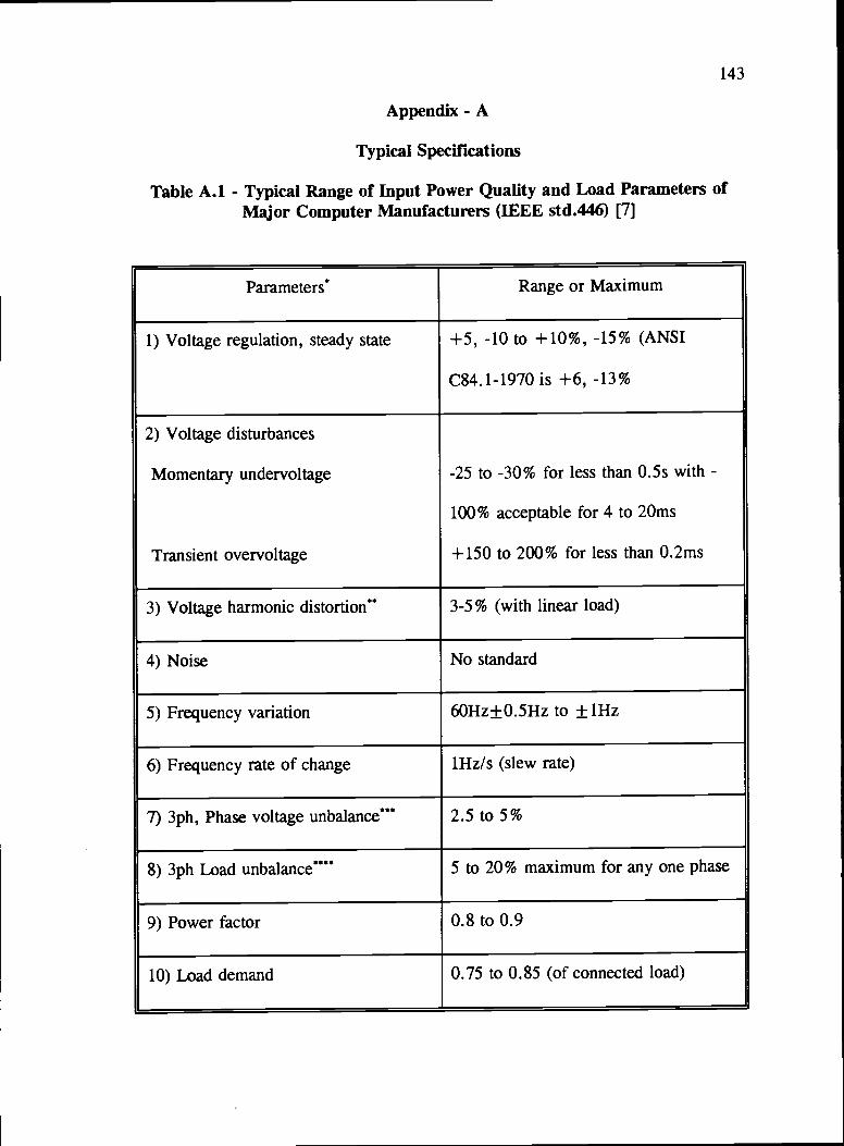
143
Appendix - A
Typical Specifications
Table A.1 - Typical Range of Input Power Quality and Load Parameters ofMajor Computer Manufacturers (IEEE std.446) [7]
Range or Maximum
1) Voltage regulation, steady state +5, -10 to + 10%, -15% (ANSI
C84.1-1970 is +6, -13%
2) Voltage disturbances
Momentary undervoltage
Transient overvoltage
-25 to -30% for less than 0.5s with
100% acceptable for 4 to 2Oms
+ 150 to 200% for less than 0.2ms
3) Voltage harmonic distortion 3-5% (with linear load)
4) Noise No standard
5) Frequency variation 6OHz±0.5Hz to ± 1Hz
6) Frequency rate of change 1Hz/s (slew rate)
7) 3ph, Phase voltage 2.5 to 5%
8) 3ph Load 5 to 20% maximum for any one phase
9) Power factor 0.8 to 0.9
10) Load demand 0.75 to 0.85 (of connected load)
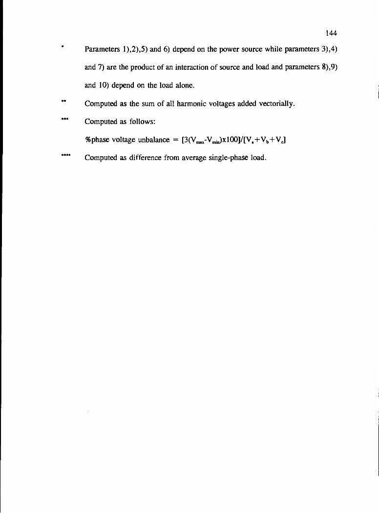
144
Parameters 1),2),5) and 6) depend on the power source while parameters 3),4)
and 7) are the product of an interaction of source and load and parameters 8),9)
and 10) depend on the load alone.
Computed as the sum of all harmonic voltages added vectorially.
Computed as follows:
%phase voltage unbalance = [3(VV)X100]/[Va+Vb+Vc]
Computed as difference from average single-phase load.

145
Appendix - B
Theory of Fuzzy Control [50-62]
Fuzzy logic, introduced by Zadeh [50], is gaining popularity in wide
applications mostly in socio-economics and process control systems. More recently,
researchers started using this concept in applications involving the electhcal machine
and power electronic circuits.
Zadeh, based on his work on fuzzy sets [51], has outlined a new approach to
the analysis of complex systems and decision processes with the following three
distinguishing features:
[1] Use of so-called 'linguistic' variables in place of or in addition to
numerical variables
[2] Characterization of simple relations between variables by fuzzy
conditional statements
[3] Characterization of complex relations by fuzzy algorithms.
A complex system often is difficult to model, but can be characterized by having
a considerable amount of essential a priori information in a qualitative form and by
having performance criteria which are specified linguistically. A fuzzy control
algorithm is used to implement this kind of linguistically expressed and poorly-defined
control policies. The fuzzy control is basically nonlinear. The adaptive nature of this
control results in nullifying the effect of the parameter or load variations.
Figure B. 1 shows the difference between an ordinary set and a fuzzy set [52].
Suppose it is necessary to specify linguistic measures of temperatures on the closed
interval [100°F,200°F] (This numerical interval, that is relevant for the description of
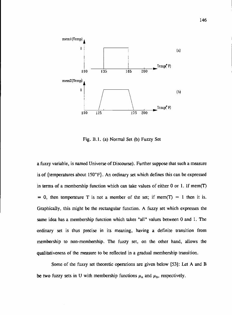
memi (Temp)
100 135 165 200
mem2(Temp)
100 125 175 200
Femp F)
rem(° F)
Fig. B. 1. (a) Normal Set (b) Fuzzy Set
(a)
(b)
146
a fuzzy variable, is named Universe of Discourse). Further suppose that such a measure
is of {temperatures about 150 °F}. An ordinary set which defines this can be expressed
in terms of a membership function which can take values of either 0 or 1. If mem(T)
= 0, then temperature T is not a member of the set; if mem(T) = 1 then it is.
Graphically, this might be the rectangular function. A fuzzy set which expresses the
same idea has a membership function which takes "all" values between 0 and 1. The
ordinary set is thus precise in its meaning, having a definite transition from
membership to non-membership. The fuzzy set, on the other hand, allows the
qualitativeness of the measure to be reflected in a gradual membership transition.
Some of the fuzzy set theoretic operations are given below [53]: Let A and B
be two fuzzy sets in U with membership functions A and /L, respectively.

147
Complement: The membership function of the fuzzy set A is pointwise defined for all
uEU by
A(u) = 1 4LL(U) (B.!)
Union: The membership function fA of the union A U B is pointwise defined
for all uEU by
(u) = max (jz(u),(u)) (13.2)
Intersection: The membership function ILAflB of the intersection A fl B is pointwise
defined for all u E U by
= mm (A(u),B(u)) (B.3)
A few more fuzzy concepts like fuzzy implication (defining fuzzy rules) and
fuzzy composition (fuzzy inference) are also required for fuzzy control algorithms.
In a fuzzy implication, the rules are generally defined in the format of IF-THEN
statements such as "If (x is A and y is B) THEN (z is C)". In most of the applications
related to machine drives and power electronics, the fuzzy variables are the error(e)
and the change in error(ce) of the output variable of a system; and the change in the
control signal(du). A given numerical value can be a member of more than one fuzzy
set and thus for a given input, more than one rule can be considered. To get a
meaningful control action out of the fuzzy controller, individual rules have to combined
and this action is defined as fuzzy composition. There are several composition methods
available but the most popular one seems to be MAX-MIN composition which is
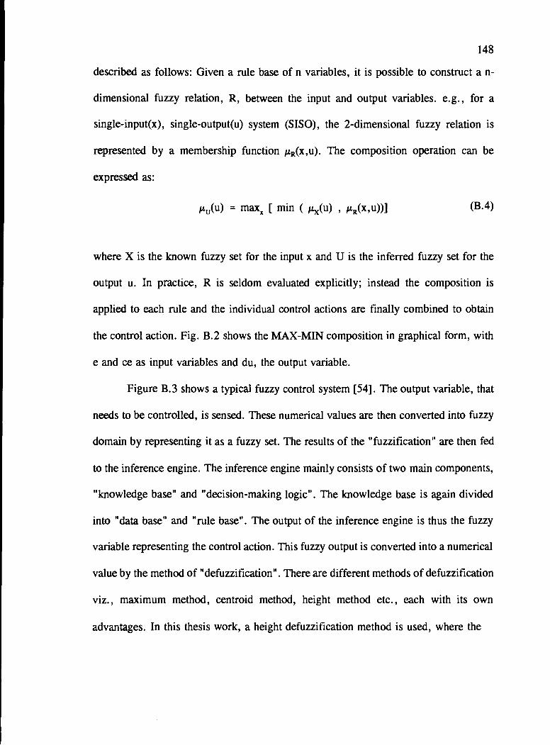
148
described as follows: Given a rule base of n variables, it is possible to construct a n-
dimensional fuzzy relation, R, between the input and output variables. e.g., for a
single-input(x), single-output(u) system (SISO), the 2-dimensional fuzzy relation is
represented by a membership function R(x,u). The composition operation can be
expressed as:
= max [ mm ( (u) , (x,u))] (B.4)
where X is the known fuzzy set for the input x and U is the inferred fuzzy set for the
output u. In practice, R is seldom evaluated explicitly; instead the composition is
applied to each rule and the individual control actions are finally combined to obtain
the control action. Fig. B.2 shows the MAX-MIN composition in graphical form, with
e and ce as input variables and du, the output variable.
Figure B.3 shows a typical fuzzy control system [54]. The output variable, that
needs to be controlled, is sensed. These numerical values are then converted into fuzzy
domain by representing it as a fuzzy set. The results of the "fuzzification" are then fed
to the inference engine. The inference engine mainly consists of two main components,
"knowledge base" and "decision-making logic". The knowledge base is again divided
into "data base" and "rule base". The output of the inference engine is thus the fuzzy
variable representing the control action. This fuzzy output is converted into a numerical
value by the method of "defuzzification". There are different methods of defuzzification
viz., maximum method, centroid method, height method etc., each with its own
advantages. In this thesis work, a height defuzzification method is used, where the
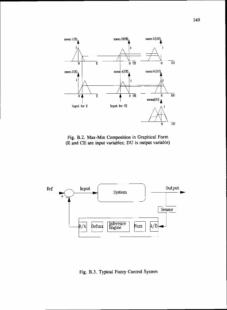
149
E L
mem
DU
mem2(E) mei 4(CE) mem6(DU)
OE DU
meni(DU)
Inpul for E Input for CE
DU
Fig. B.2. Max-Mm Composition in Graphical Form(E and CE are input variables; DU is output variable)
p
Sensor
/A uz Inferenc /D
Fig. B.3. Typical Fuzzy Control System

150
weighted (membership value) average of all the individual corrective control actions is
taken as the most typical crisp value of the fuzzy quantity.
Manidani [55] has for the first time applied the concept of fuzzy control to an
industrial process. The pressure and temperature of a steam engine (dynamic plant)
were controlled based on the concept of fuzzy logic and using maximum defuzzification
resulting in a satisfactory operation.
In a process control application, many a time the fuzzy controller is
implemented by forming a look-up table of the input variables, e and Ce, with the
output variable, du making up the matrix elements. MacVicar-Whelan [56] has shown
that in the limit as quantization levels of the control and measurement of fuzzy
variables become infinitely fine, this fuzzy controller approaches a deterministic P1
controller. Three meta-rules of representing the rule base, based on a required dynamic
response for a regulatory control, is as follows:
[1] If both e and cc are zero, then maintain the present control setting.
[2] If conditions are such that e will go to zero at a satisfactory rate, then
maintain present control setting.
[3] If e is not self correcting, then control action du is not zero and depends
on the sign and magnitude (small, medium, large etc.) of e and cc.
Although the above control objectives are typical of most industrial applications,
a conventional controller can not handle all three of them unless extended by some
additional heuristic logic. On the other hand, an experienced process operator can
easily meet all three control objectives [57].

151
A conventional P1-controller uses an analytical expression of the following form
to compute the control action
u = K e + K1 Je dt (B.5)
Differentiating this equation with respect to time,
(B.6)dt dt
Discrete time version of this equation is,
iu(k) = Kze(k) + K1e (B.7)
where
u(k) is the change of control output, where u(k) is the control output, and we
have that
u(k) = u(k) u(k-1)
e(k) is the error and we have that
e(k) = y1f y(k)
where y(k) is system output and y is the set point
e(k) is the change of error and we have that
ie(k) = e(k) e(k-1)
k is the kth sampling time.
The control objectives listed earlier would require variable gains near the set
point i.e., small K near the y and a very large K, near the constraint. Thus a simple
P1-controller is inherently incapable of achieving all of the above control objectives and

152
has to be implemented with the help of additional heuristic logic which would allow the
desired gain adaptations.
More recently, stability issues of fuzzy feedback control methods are being
looked into using such methods as state-space approach, robustness indices, input-
output stability and circle criterion [58]. Also, stability studies using nyquist criterion
is reported [59].
Apart from the points enumerated above, from an implementation point of view,
the strength of fuzzy control is that the number of rules required to express the fuzzy
relation is fairly small and thus the memory requirement is low compared to large look-
up tables needed in conventional methods. In spite of the advantages in fuzzy control,
the following limitations/difficulties are noted [40]:
[1] Lack of systematic design procedure and difficulty in analysis.
[2] Lack of completeness of rule base, because the controller needs to
output a reasonable value for every input operating condition of the
process.
[3] No definite criteria for selection of the shape of membership functions,
degree of overlapping of fuzzy sets and the quantization levels.


![[d], [o] If one doctor doctors another doctor does the doctor who doctors the doctor doctor the doctor the way the doctor he is doctoring doctors? Or](https://img.dokumen.tips/doc/110x75/56649e995503460f94b9c732/d-o-if-one-doctor-doctors-another-doctor-does-the-doctor-who-doctors-the.jpg)