UNIVERISTY OF TARTU

FACULTY OF MATHEMATICS AND COMPUTER SCIENCE

Institute of Computer ScienceInformation Technology Curriculum

Martin Loginov

Beyond decoding: representational similarityanalysis on fMRI data

Master’s Thesis (30 EAP)

Supervisor: Raul Vicente Zafra, PhD

Tartu 2015

Beyond decoding: representational similarity analysis on fMRIdata

Abstract:Representational similarity analysis is a novel data analysis technique in neurosciencefirst proposed by Kriegeskorte et al. in [KMB08]. It aims to connect different branchesof neuroscience by providing a framework for comparing activity patterns in the brainthat represent some cognitive processes. These activity patterns can come from varioussources, like different subjects, species or modalities like electroencephalography (EEG)or functional magnetic resonance imaging (fMRI). The central concept of RSA lies inmeasuring the similarity between these activity patterns. One of the open questionsregarding RSA is what distance measures are best suited for measuring the similaritybetween activation patterns in neuronal or fMRI data.

In this thesis RSA is implemented on a well known fMRI dataset in neuroscience,that was produced by a studying the categorical representations of objects in the ventraltemporal cortex of human subjects [HGF+01]. We carry out RSA on this dataset usingdifferent notions of distance and give an overview of how the end results of the analysis areaffected by each distance notion. In total 9 different distance measures were evaluated forcalculating the similarity between activation patterns in fMRI data. The results providedin this thesis can be used by researchers leveraging RSA to select distance measures fortheir studies that are most relevant to their particular research questions at hand. Inaddition to the comparison of distance notions, we also present a novel use case for RSAas a tool to visualize the global effects different transformations can have on the inputdataset.

Keywords: representational similarity analysis, fMRI, ventral temporal cortex, distancemeasures

2

Dekodeerimise tagamaad: fMRI andmete esituste sarnasuse analuus

Luhikokkuvote:Andmeesituste sarnasuse analuus on uudne andmeanaluusimeetod neuroteaduste kon-tekstis, mis pakuti valja Kriegeskorte et al. poolt artiklis [KMB08]. Selle eesmargikson uhendada erinevaid neuroteaduste harusid, luues uhtne raamistik erinevaid kognitiiv-seid protsesse esindavate aktiivsusmustrite omavaheliseks vordlemiseks ajus. Raamistikvoimaldab omavahel vorrelda tegevusmustreid, mis parinevad erinevatest allikatest, naguerinevatelt katsealustelt, liikidelt voi on moodetud kasutades erinevaid tehnoloogiaid naguelektroentsefalograafia (EEG) voi funktsionaalse magnetresonantstomograafi (fMRI) abi.Andmeesituste sarnasuse analuusi keskne idee seisneb nende mustrite omavahelise sar-nasuse vordlemises. Uks lahtisi kusimusi selles valdkonnas seisneb sobivate moodikuteleidmises funktsionaalse magnetresonantstomograafi poolt moodetud aktiivsusmustriteomavahelise sarnasue hindamiseks.

Kaesolev magistritoo viib labi andmeesituste sarnanuse analuusi uhe neuroteadustesteada tuntud fMRI andmestiku peal [HGF+01]. Analuusi kaigus uuritakse erinevate kau-gusmoodikute moju andmeesituste sarnasuse analuusi lopptulemustele ja antakse sellestpohjalik ulevaade. Kokku on uurimise all 9 erinevat kaugusmoodikut. Kaesoleva tootulemusena valmib pohjalik ulevaade erinevate kaugusmoodikute mojust andmeesitustesarnasuse analuusile, mida on voimalik kasutada edasistes neuroteaduse alastes uurnguteshindamaks erinevate kaugusmoodikute sobivust mone konkreetse uurimustoo kontekstis.Lisaks kaugusmoodikute vordlemisele pakub kaesolev too valja ka uhe uudse kasutusjuhuandmeesituste sarnasuse analuusile. Nimelt on voimalik konealust meetodit kasutada kaerinevate lahteandmetele rakendatavate teisenduste moju visuaalseks hindamiseks.

Votmesonad: admeesituste sarnasuse analuus, funktsionaalne magnetresonantstomo-graafia, kaugusmoodikud

3

Contents

1 Introduction 5

2 Background information 72.1 What is MRI . . . . . . . . . . . . . . . . . . . . . . . . . . . . . . . . . 72.2 fMRI . . . . . . . . . . . . . . . . . . . . . . . . . . . . . . . . . . . . . . 8

3 Methods 93.1 Obtaining the data . . . . . . . . . . . . . . . . . . . . . . . . . . . . . . 93.2 The dataset: neural responses to grayscale images . . . . . . . . . . . . . 93.3 Software used for processing the data . . . . . . . . . . . . . . . . . . . . 113.4 Preparing the fMRI data for analysis . . . . . . . . . . . . . . . . . . . . 123.5 Region of interest - ventral temporal cortex . . . . . . . . . . . . . . . . . 143.6 Classification analysis . . . . . . . . . . . . . . . . . . . . . . . . . . . . . 163.7 Representational similarity analysis . . . . . . . . . . . . . . . . . . . . . 193.8 Ordering representational dissimilarity matrices using hierarchical clustering 223.9 Dimensionality reduction using multidimensional scaling . . . . . . . . . 233.10 Different notions of distance . . . . . . . . . . . . . . . . . . . . . . . . . 26

3.10.1 Bray-Curtis distance . . . . . . . . . . . . . . . . . . . . . . . . . 263.10.2 Canberra distance . . . . . . . . . . . . . . . . . . . . . . . . . . . 263.10.3 Chebyshev distance . . . . . . . . . . . . . . . . . . . . . . . . . . 263.10.4 Cityblock distance . . . . . . . . . . . . . . . . . . . . . . . . . . 263.10.5 Correlation distance . . . . . . . . . . . . . . . . . . . . . . . . . 263.10.6 Cosine distance . . . . . . . . . . . . . . . . . . . . . . . . . . . . 273.10.7 Euclidean distance . . . . . . . . . . . . . . . . . . . . . . . . . . 273.10.8 Hamming distance . . . . . . . . . . . . . . . . . . . . . . . . . . 273.10.9 Mahalanobis distance . . . . . . . . . . . . . . . . . . . . . . . . . 273.10.10 Kendall’s tau . . . . . . . . . . . . . . . . . . . . . . . . . . . . . 27

4 Results 294.1 Validating the region of interest . . . . . . . . . . . . . . . . . . . . . . . 294.2 Classical representational similarity analysis . . . . . . . . . . . . . . . . 304.3 The effect of distance on RSA . . . . . . . . . . . . . . . . . . . . . . . . 364.4 RSA as a tool for assessing data quality . . . . . . . . . . . . . . . . . . . 43

5 Discussion 45

6 Conclusions 47

4

1 Introduction

The human brain is one of the most complex biological structures in existence. Theinner workings of this incredible organ, that is responsible for every single thought orcomplex cognitive process in humans and animals alike, have for long been the subjectof scientific study in many different fields. One on the key questions in neuroscience isdetermining how the brain represents different types of information. Studies have shownthat different areas in the brain are associated with different types of information. Thereare specific regions associated with the processing of low level visual information (Vu etal. [VRN+11]), while other areas process information on a more abstract level, dealingwith the categorization of objects (O’Toole et al. [OJAH05]; Haxby et al. [HGF+01]).

While it is known that information processing differs between brain regions, little isknown about the exact nature of information representation in these different regions orhow a set or neurons maintain information. To alleviate some of the shortcomings ofexisting analysis techniques in neuroscience, a novel method was proposed in a paper byKriegeskorte et al. called representational similarity analysis [KMB08]. RSA provides arobust framework for studying how different stimuli or cognitive processes are representedin the brain. It has since been used to study how the categorical representation of objectsdiffers between humans and monkeys for example [KMR+08].

While RSA is showing great promise in connecting different branches of neuroscience,there are also numerous questions still open. The central concept of RSA lies in measuringthe similarity between activity patterns in the brain. These activity patterns can bemeasured using different technologies, for example by directly measuring the electricalactivity from the brain using electroencephalography (EEG) or by indirectly measuringblood flow using functional magnetic resonance imaging (fMRI). In both cases the activitypatterns themselves are composed of information coming from different channels (in thecase of EEG) or different voxels (for fMRI) - they are multivariate. One of the corequestions raised in a recent review article by Kriegeskorte et al. is: ”What multivariatedistance is best suited for measuring representational dissimilarities in neuronal or fMRIdata?” [KK13]

This thesis aims to study the effects of different notions of distance in measuring thesimilarity between activity patterns that make up neural representations in the context offMRI data. Our goal is to assess how the different distance measures influence the resultsof representational similarity analysis for activation patterns in fMRI data. In total weevaluate nine different notions of distance by implementing representational similarityanalysis with each of them on a well known fMRI dataset in neuroscience [HGF+01].The results presented here can be used to enhance the utility of RSA as a analysistechnique in neuroscience. By providing a thorough overview of the effects resulting fromdifferent distance measures we provide researchers the ability to select for their analysisthe distance measures that are most relevant to their particular research questions.

The bulk of this thesis is organized very coarsely into four core chapters:

• Chapter 2 provides some background to readers completely unfamiliar with neu-roimaging techniques. This is done to provide a better understanding of the datasetused in this thesis.

• Chapter 3 gives a thorough overview of all the different steps involved in the anal-ysis for this thesis. It starts with the description of the dataset and preprocessingsteps, familiarizes the reader with the concepts of classification analysis and rep-

5

resentational similarity analysis and ends with the description of all the differentnotions of distance we evaluated in this thesis.

• Chapter 4 contains all the results obtained from different analysis stages. Thereader is presented with the results from classification analysis, followed an examplerepresentational similarity analysis. The bulk of this chapter consists of the resultswe obtained testing different notions of distance. In the end we also present a noveluse case for representational similarity analysis we discovered while doing researchfor the thesis.

• Chapter 5 tries to present some possible interpretations for the results obtained inthis thesis and the reasoning behind them. Some ideas for further research are alsoproposed.

6

2 Background information

This section tries to provide some background information to a reader completely unfa-miliar with brain imaging techniques. The main goal here is not to provide a thoroughtechnical overview, but rather convey some intuition about what can be accomplishedwith different brain imaging techniques and how they can be used for measuring brainactivity.

2.1 What is MRI

MRI stands for magnetic resonance imaging and is a technique for creating detailedimages of organs and other types of soft tissue inside an organism. An MRI scannerworks by applying a very strong magnetic field to the atoms making up the differenttissues. ”The magnetic field inside the scanner affects the magnetic nuclei of atoms.Normally atomic nuclei are randomly oriented but under the influence of a magneticfield the nuclei become aligned with the direction of the field. The stronger the field thegreater the degree of alignment. When pointing in the same direction, the tiny magneticsignals from individual nuclei add up coherently resulting in a signal that is large enoughto measure.” [Dev07]

The magnitude of this summary signal varies between different types of tissue - this isthe key concept behind MRI technology that facilitates the creation of detailed anatomicalimages. When used for brain scans, this variability in signal strength makes it possibleto differentiate between between gray matter, white matter and cerebral spinal fluid instructural images of the brain. You can see what an MRI scan looks like on Figure 1.

Figure 1: Single slice from a brain MRI scan [Slo13]

The image obtained as a result of a scan is actually 3-dimensional. This point is

7

illustrated on Figure 1 as it shows only a single slice cut through the brain and there aremany such slices on different levels.

The entire image is made up of tiny units called voxels 1. Depending on the scannerand scan type the size of a voxel can vary from less than a cubic millimetre to a coupleof cubic millimetres, therefore encompassing brain tissue consisting of millions of cells.The size of a voxel effectively determines the resolution of the resulting image. Thehigher the resolution, the more time it takes for the scanner to create a full brain image.This limitation becomes important when taking functional images (see Section 2.2) andis usually the reason why functional images are created with a lower resolution thananatomical images.

2.2 fMRI

While MRI facilitates the creation of detailed images of brain anatomy, fMRI (functionalmagnetic resonance imaging) provides the ability to indirectly measure brain activity.Functional imaging is an enhancement to the regular MRI technique to account for bloodflow inside the brain.

The underpinnings of modern fMRI were first discovered by Seiji Ogawa. Whileconducting research on rat brains, he was trying out various different settings on hisMRI scanner and discovered a contrast mechanism reflecting the blood oxygen level ofdifferent brain tissue [Log03]. Today, Ogawa’s discovery is known as blood oxygen level-dependent signal (BOLD). It is also known that BOLD contrast depends not only onblood oxygenation but also on cerebral blood flow and volume.

These changes in blood flow, volume and oxygenation, that are linked to some neuralactivity are known as the hemodynamic signal. Cognitive processes in the brain consistof millions of neurons firing. Unlike electroencephalography (EEG) which measures elec-trical activity from the neurons more or less directly, the hemodynamic BOLD signal isa indirect measure of neural activity. This thesis does not concern itself with the exactneuroscientific semantics of the link between the BOLD signal and brain activity. Forour intents and purposes we just consider the BOLD signal to be influenced by neuralactivity in a way that a change in the signal in interpreted as a change in neural activity.

The data from fMRI experiments is a set of 3D volumes consisting of voxels. Eachvoxel has an intensity value that represents the BOLD signal in that particular area of thebrain. During a scan session hundreds of such 3D volumes are recorded, usually while thesubject is performing some task. These volumes together form a timeseries and representthe change in the hemodynamic signal in time and are the subject for analysis in thisthesis.

1A voxel or volumetric pixel can be thought of as the 3-dimensional equivalent to a 2-dimensionalpixel.

8

3 Methods

This chapter provides a detailed overview of all the data analysis techniques used inthis thesis. For starters we describe how the data was obtained, the experiment thatproduced it, followed by a detailed description of preprocessing steps to make it viable forstatistical analysis. Before describing the core concepts behind classification analysis andrepresentational similarity analysis, we also give an overview how and why we localizedthe core analysis steps to a particular region in the brain. The chapter ends with thedescriptions of all the different notions of distances we evaluated for this thesis.

Readers not particularly interested in all the technical details can skip this chapterand go straight to chapter 4 that contains all the results from the different analysis stepsdescribed in this chapter. Relevant details from this chapter are also referenced fromthere.

3.1 Obtaining the data

The data used in this thesis was acquired from the OpenfMRI project [PBM+13] database.OpenfMRI aims to provide researchers a common platform and infrastructure to maketheir neuroimaging data freely available to any interested party.

The project tries to solve some of the big challenges with sharing fMRI datasets exist-ing today, like the large size of datasets and lack of standardization in data organizationand preprocessing steps. By providing a common format to organize different types ofdata (imaging data, experimental task descriptions, behavioural data) and tools for pre-processing the data, they are greatly simplifying the process of obtaining datasets forneuroscientific studies.

3.2 The dataset: neural responses to grayscale images

The specific dataset we used was produced for a study by Haxby et al. [HGF+01], wherethey studied the representations of faces and objects in the ventral temporal cortex ofhuman subjects. This section will give a thorough overview of their experiment and thedata produced.

During the experiment neural responses were collected from six subjects (five femaleand one male) using a General Electric 3T fMRI scanner while they were performing a one-back repetition detection task. In essence subjects were presented with different stimuliconsisting of gray-scale images that depicted objects belonging to different categories (seeFigure 2) and for each stimulus image the subjects had to indicate whether the imagewas the same or different as the previous image.

By design the experiment was a block design experiment. This is one of the twocommon types of experiments used to gather fMRI data (the other being event-relateddesign) [AB06]. In a block design experiment two or more conditions are being presentedto the subject in alternating blocks and in each block only one condition is active. Duringeach block a certain number of fMRI scans are taken and these scan volumes will representthe neural responses for the condition at hand. The blocks are usually separated by aperiod of rest to allow the hemodynamic signal to return to a baseline. This makes iteasier and more robust to distinguish the signals representing different conditions.

In this specific experiment the condition for a block was the category of a stimulusimage. Stimuli were gray-scale images of faces, houses, cats, bottles, scissors, shoes,

9

Figure 2: Examples of stimuli. Subjects performed a one-back repetition detection taskin which repetitions of meaningful pictures were different views of the same face or object.[HGF+01]

chairs and nonsense patterns - eight different categories in total. Twelve time serieswere obtained for each subject. Each time series began and ended with 12s of rest andcontained eight stimulus blocks of 24-s duration, one for each category, separated by 12-sintervals of rest. An illustration of a single time series (a singe run of the experiment) isshown on Figure 3.

Stimuli were presented for 500 ms with and interstimulus interval of 1500 ms. Rep-etitions of meaningful stimuli were pictures of the same face or object photographedfrom different angles. Stimuli for each meaningful category were four images each of 12different exemplars.

For each timeseries 121 3-dimensional fMRI volumes were obtained with dimensionsof 40 x 64 x 64 voxels. With the scan parameters used2 each voxel represents the neural

2repetition time (TR)=2500 ms, 0 3.5-mm-thick sagittal images, field of view (FOV) = 24 cm, echotime (TE) = 30 ms, flip angle = 90

10

Figure 3: Depiction of the different stimulus blocks in a single time series of the experi-ment. Time is shown on the horizontal axis from the start of the run.

activity in an area of brain tissue the size of 3.5 x 3.75 x 3.75 mm. The count of volumesfor each series (121) comes from the fact that under these scan parameters (specificallythe repetition time (TR) = 2500 ms) it takes 2.5 seconds to carry out a full brain scan.The last scan is initiated after the final 12s of rest in each timeseries (after timepoint300s).

Each of the scan volumes is a representation of either one of the active experimentconditions (category of a stimulus) or the resting state and is labeled accordingly. Thevoxel values in these scan volumes together with the labels serve as input to analysis inthis thesis.

It might seem surprising to the reader that nothing is done with the results of theone-back repetition detection task - in fact this kind of behavioural data is not evenincluded in the OpenfMRI database for this dataset. The main goal of the one-backtask is actually to trick the subjects into concentrating on the individual images whichwould allow them also to perceive the category of the image. Without this kind of taskat hand the attention of the subjects would likely dissipate at least once during the fiveminute test run and this kind of background activity from wandering thoughts would addadditional noise to the scan results.

3.3 Software used for processing the data

Right from the beginning of this project we decided to use IPython Notebooks as ourmain analysis platform [PG07]. Having the ability to run arbitrary Python code onremote servers conveniently through a web browser proved invaluable to us when thememory and computation requirements of the analysis exceeded the capacity of a singlelaptop. Python’s large ecosystem of 3rd party libraries coupled with IPython Notebook’sability to visualize plots in-line with the actual code and notes make it a very productiveand accessible environment for exploratory data analysis.

The other main reason besides accessibility for choosing this analysis platform wasthe existence of the PyMVPA toolbox (MultiVariate Pattern Analysis in Python). Theauthors describe it as: ”a Python package intended to ease statistical learning analysesof large datasets. It offers an extensible framework with a high-level interface to a broadrange of algorithms for classification, regression, feature selection, data import and export.” [HHS+09]

PyMVPA abstracts away much of the complexities associated with analyzing neu-roimaging data. It provides functions for directly loading in datasets that are structuredaccording to the OpenfMRI specification [PBM+13] and provides numerous means for

11

preprocessing them. Scaffolding for running cross-validated classification and representa-tional similarity analysis is also provided, which is leveraged extensively by the analysissteps in this thesis.

A similar toolbox to PyMVPA exists that is targeted specifically to carrying out repre-sentation similarity analyses in Matlab, as described in a paper by Nili et al. [NWW+14a].Although the paper describes it to be somewhat similar with respect to RSA functional-ity, it lacks the additional features and flexibility of PyMVPA. In addition, Matlab is aproprietary platform which would have required us to deal with licensing issues.

Besides PyMVPA another notable piece of software in our analysis pipeline is theScikit-Learn machine learning library for Python [PVG+11]. It is a library that pro-vides simple and efficient tools for data mining and data analysis. Besides the fact thatPyMVPA uses it internally for classification analyses for example, we also use it directlyto carry out dimensionality reduction leveraging the results of representational similarityanalysis.

For visualizing the raw fMRI data the MRIcron toolkit was used [RKB12]. Thistoolkit was used to visualize region of interest maps and the results of our experimentswith searchlight analysis (see Section 3.5).

3.4 Preparing the fMRI data for analysis

The output of most fMRI experiments is a number of 3D scan volumes (images from nowon) for each run of the experiment. Each image just contains the raw BOLD intensitiesfor each voxel and represents the neural activity for the entire scan area (usually thewhole brain) at a particular timepoint. To make any meaningful statistical analysis onthese images viable, a number of preprocessing steps need to occur to transform the rawdata.

This section gives an overview of the preprocessing steps carried out on the dataset toprepare it for analysis. We divide the steps into two: some are ”standard” preprocessingtechniques, that are performed on most fMRI datasets before analysis and are in factalready applied for all datasets in the OpenfMRI database, the other steps we appliedourselves with respect to our particular analysis. As the technical details for the formerare beyond the scope of this thesis, we only give a list of the more important steps for thesake of completeness and describe each step briefly in terms of its input and output, formore thorough explanations refer to [Str06]. Some of the more important preprocessingsteps in the order they are implemented:

1. Conversion of file formats: as data can come from different scanners that usedifferent formats, everything is converted into a common format - NIfTI (Neu-roimaging Informatics Technology Initiative file format [CAB+04]). This is done tofacilitate inter-operation of different functional MRI data analysis software.

2. Motion correction: subjects inevitably make small movements during experi-ments. This causes the signal-to-noise ratio of the resulting scan images to drop.Motion correction is used to calculate a set of rigid body transformations for eachimage to counteract this.

3. Brain extraction: the scanner itself has no means to distinguish between thebrain and other tissue types. Brain extraction is later used as a preprocessing stepto extract from the images an image mask representing only the voxels that containactual brain tissue.

12

The above list is not meant to be a comprehensive enumeration of all the steps thatwent into preprocessing the raw data, it is merely there to give the reader a glimpse ofdifferent types of methods that need to be used before any higher level analysis can occur.Preprocessing fMRI data is a complex field - entire university courses are taught on thesubject. Next we describe a set of steps taken during the analysis of this thesis and addsome reasoning for each step.

Since the spacial structure of images is not really needed in any parts of the analysis(after applying region of interest masks as described in Section 3.5) all the images areconverted into vectors of voxel intensities by simply concatenating all the voxel values ina volume:

image = [v1, v2...vn]

Here v1 through vn are the individual voxel intensities. Representing the images like thismakes working with the data much simpler because it is much clearer to reason in termsof vectors for most data analysis algorithms, than it would be for 3D volumes.

Even after motion correction, the data can still contain some global effects, like lowfrequency signal intensity drift in the intensity values of voxels throughout a timeseries.This phenomenon is described in a technical paper by Tanabe et al. where they say thattwo known sources of drift are noise from the MR scanner and aliasing of physiologicalpulsations [TMT+02]. The paper centers around the issue that there is not yet a clearconsensus on which algorithm should be used for removing these sorts of drifts andpresents the comparison of a few methods.

In this thesis we used a technique called detrending, provided by the PyMVPAtoolkit [HHS+09]. The main idea behind detrending is modeling the drifts in intensi-ties as polynomial trends. It basically transforms the data by fitting polynomials to thetimeseries of each voxel, leaving only information that is not explained by the polynomi-als. In the simple case of linear detrending, a straight line is fit through the timeseriesof a voxel using linear regression and the voxel initensity values are replaced with theresiduals from the regression.

After detrending we would like to increase the signal to noise ratio for the data evenmore by trying to focus on the parts of the signal that are related to the stimuli. For thiswe transform the timeseries of each voxel so that it no longer contains the raw BOLDsignal intensities, but a deviation from a baseline signal. The idea behind this is that weonly want to focus on activity elicited by a stimulus, not on activity that is there all thetime. In our case, the resting state will serve as the baseline. This technique is calledz-scoring, although the classical version differs from the variation presented here:

1. The timeseries of each voxel is considered separately from all the others. A time-series for a voxel is composed of all the values for this single voxel for a specific runof the experiment.

2. Calculate the mean intensity value of the voxels for resting state only.

3. Calculate the standard deviation of intensity values of the voxels for resting stateonly.

4. For all the voxels in a timeseries, calculate the deviation from the mean calculatedin step 2 in units of standard deviation, step 3.

After z-scoring, we remove all images for resting state from the dataset. This is donebecause resting state images are not interesting (nor particularly useful after z-scoring has

13

been carried out), since all subsequent analysis stages deal only with the representationsof the different stimuli.

The final output from the preprocessing stage for a single subject comprises of 864image vectors each containing the the voxel intensities of about 500 voxels, as defined bythe region of interest. This number of images takes into account images from all the 12time series with resting state images removed.

3.5 Region of interest - ventral temporal cortex

In our dataset each fMRI volume in a timeseries contains over 160 000 voxels that makeup the neural representation of the entire brain at a single point in time. Processingthis amount of data is not actually a problem with the computational resources readilyavailable today, although some types of analysis using these full brain images can still takea long time, for example classification analysis. Still we confine all subsequent analysisimplemented in this thesis to only a particular region in the brain, for reasons that willbe explained in the following paragraphs.

At all times, even during seemingly restful periods, there are always some backgroundcognitive processes happening in the brain that cause the firing of millions of neurons.These firings cause changes in the hemodynamic BOLD signal that is measured by thefMRI scanner. Some of these cognitive processes can be localized to specific areas inthe brain [PPFR88] while others seem to occur globally. In addition it is known thatthe representation of the same information can differ greatly between different brainregions[NPDH06]. As we are interested in only the representations of categories of visualobjects, activity from all these other processes become noise in the dataset with respectto our goals. Therefore we would like to localize our analysis to a region in the brain thatwe know contains the neural representations of the particular conditions or phenomenathat are of interest to us - this is known as a region of interest in neuroscience. This sortof localization is important because the data coming from the fMRI scanner is inherentlynoisy, distinguishing our signal from all the other processes in the entire brain would bevery difficult if not impossible.

A ROI can be defined either anatomically or functionally. An anatomically definedregion is an area in the brain that is known from previous studies or research to containthe neural representation of interest. In practice for fMRI datasets, regions of interestare defined by masks. A mask represents the notion that from all the voxels in the brain,we select only the ones belonging to our ROI and mask the others. Masks are carefullydrawn for each subject (as each brain is unique to a certain extent) by neuroscientistsusing landmarks in the brain that are common to all animals in a species. In this thesisthe region of interest was also chosen anatomically to be the ventral temporal cortex inthe brain, shown on Figure 4.

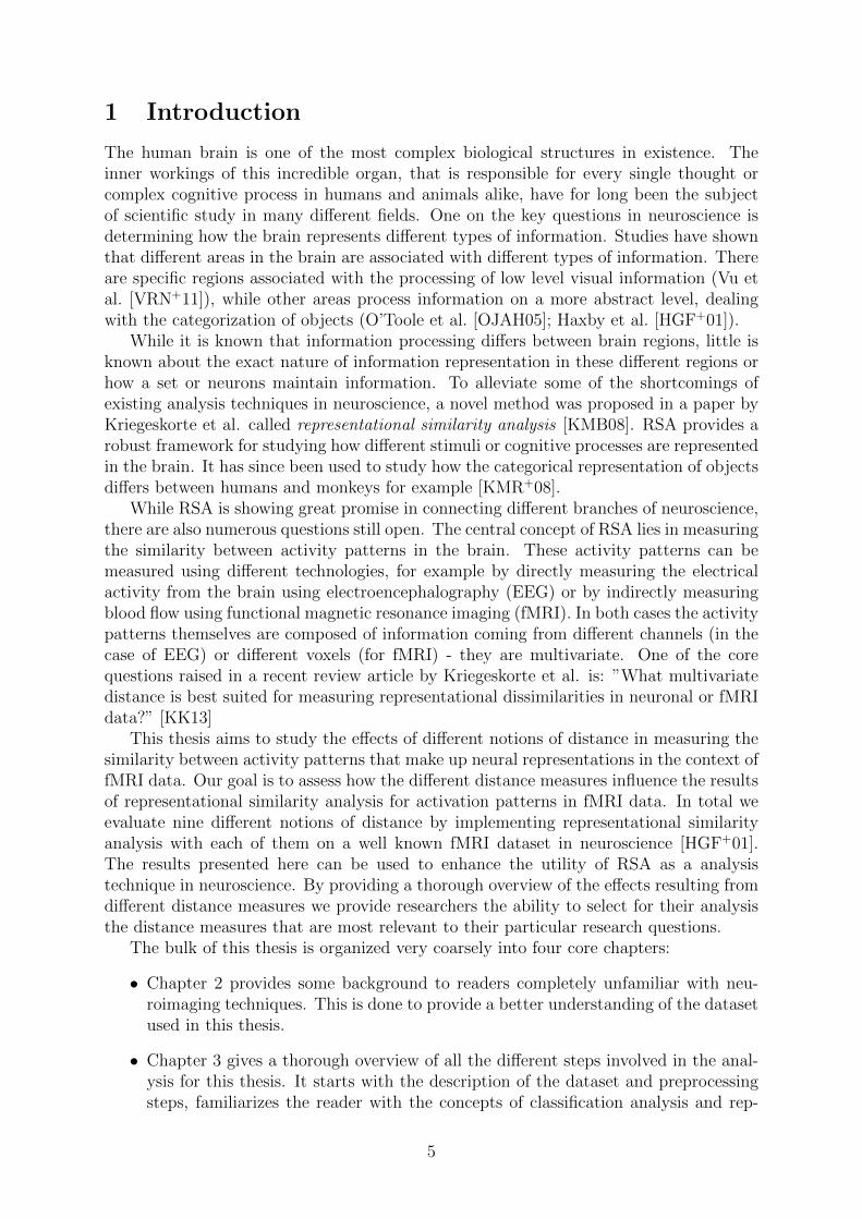
The ventral temporal cortex in humans has been extensively studied and is known torepresent visual stimuli in an abstract manner that allows these stimuli to be groupedinto different categories. Some studies that have shown this categorical organization ofrepresentations include [OJAH05] and [HMH04] among others. For the dataset used inthis thesis the ventral temporal cortex consists of 577 voxels.

During research for this thesis we also tried to define our region of interest function-ally. This begins by first hypothesising that there is a specific area in the brain wherethe information of interest (categories of objects) is represented in a way that is relevantto our analysis. In our case we would like that the representations of different cate-

14

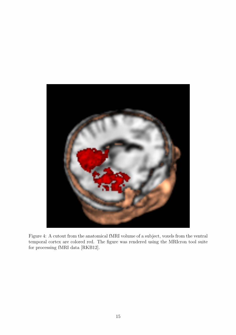
Figure 4: A cutout from the anatomical fMRI volume of a subject, voxels from the ventraltemporal cortex are colored red. The figure was rendered using the MRIcron tool suitefor processing fMRI data [RKB12].

15

gories are clearly separable from each other. To find this region we used a techniquecalled searchlight analysis, as proposed by Nikolaus Kriegeskorte and Peter Bandettiniin [KB07]. Searchlight analysis takes into account the spacial structure of fMRI volumesand is composed of the following steps:

1. Define a radius as a number of voxels. This radius will determine the size ofthe area (in voxels) that is considered for each iteration in the analysis.

2. Iterate over all the voxels in the dataset. In our case we have 40 ∗ 64 ∗ 64 =163840 for a single fMRI volume. On each iteration we only consider voxels thatare in the immediate vicinity of the current voxel at hand, as defined by the radiusin step 1. This essentially allows us to move through the entire brain and localizeall our processing to a small area in each iteration. In fact the term searchlightanalysis originates from the notion that in essence we are looking for somethingin the brain by casting a figurative searchlight (our region defined by the radius)around the entire brain and examining things we can observe in the light.

3. Calculate a metric for each region to assess the relevancy of this partic-ular area for the research question at hand. In our case we ran classificationanalysis as described in Section 3.6 to determine how well the representations ofdifferent categories are separated in a specific region. A high classification accuracyin identifying fMRI volumes that contain the representation of a particular stimuluscategory would indicate the suitability for further analysis of this region.

As a result of searchlight analysis, the region we found (with the highest overallclassification accuracy in identifying different categories) was to a large extent overlappingwith the ventral temporal cortex defined anatomically. Since the average classificationaccuracy in this functional region was only marginally higher than in the ventral temporalcortex, we opted to use the anatomically defined region for all subsequent analysis instead.

This decision in favor of using the anatomical region was influenced by two factors.First there are numerous pitfalls and limitations in interpreting the results from regionsdefined by searchlight analysis in a neuroscientifically meaningful way. The discussionof these limitations is beyond the scope of this thesis, but is covered by Etzel et al.in [EZB13]. Second, since data from the ventral temporal cortex in the same datasetwe used is already extensively studied, as mentioned above, we wanted our results to bedirectly comparable with the previous studies. Defining a different region would havemade direct comparisons more difficult while at the same time giving us no additionalbenefits.

3.6 Classification analysis

As a result from the preprocessing stage we obtained 864 vectors with fMRI image data.These vectors each contain the neural representation of a particular stimulus categoryand are labeled accordingly. Before we can go on to study the representations directly, wehave to make sure that this dataset contains enough information to distinguish betweenrepresentations of different categories in the experiment. In other words we would like toknow if images for different categories would still be distinguishable from each other ifthey were not labeled.

For this purpose we train a classifier. From a very high level perspective a classifieris a function that is trained to identify samples from a dataset based on some features.

16

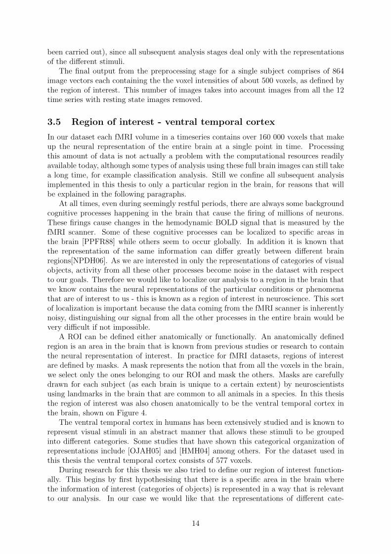
In our particular case the samples are the images and the features are individual voxelvalues. A set of samples together with their label are used as input to train the classifier(Figure 5).

Figure 5: Depiction of a dataset consisting of samples used for the training procedure ofa classfier. Figure adapted from [PMB09].

There are many different types of classifiers and they all work differently, but theirgeneral concept of operation is similar. They contain some internal parameters whichare tuned according to the training dataset. These parameters are supposed to capturethe underlying structure of the data based on the features. The idea is that if a classifiermanages to capture the underlying structure in the data, then it can use it to predictlabels for samples it has never seen before. Given a sample x = [x1...xn] the classifier fwould predict it’s label y:

y = f(x)

To assess the quality of a classifier, it needs to be tested on a different set of samplesfrom the ones used to train it. ”The typical assumption for classifier learning algorithmsis that the training (and testing) examples are independently drawn from an ‘exampledistribution’; when judging a classifier on a test set we are obtaining an estimate of itsperformance on any test set from the same distribution [PMB09].” The process of trainingand evaluation of a classifier is depicted on Figure 6.

Figure 6: Classifier training and evaluation [PMB09].

To actually measure the quality of a classifier function we calculate a metric calledclassification accuracy :

n∑i=1

I(f(xi), yi)

n(1)

17

Here n is the number of samples in the test set, xi and yi are the ith sample vectorand label from the test set respectively and I is a function returning 1 if f(xi) = yiand 0 otherwise. In other words classification accuracy is the ratio of correctly classifiedsamples from the test set to all the samples in the test set.

Partitioning data samples into training and test sets for validation can be done ina multitude of ways. Ideally we would like to have as many samples as possible fortraining the classifier to make it more accurate, while still having a test set that is agood representative sample of the entire dataset. In order to achieve this we opted for atraining/test procedure called cross-validation.

The idea behind cross-validation (also sometimes called n-fold cross-validation) is topartition the entire dataset into n folds. It is imperative that each fold contains the sameproportion of samples from all the different classes, to help the classifier capture thestructure of the different samples as equally as possible. After partitioning the followingprocedure is implemented, which is also illustrated on Figure 7:

1. Leave one of the folds out and train the classifier using samples from all the othern− 1 folds. Use the data from the left out fold for testing.

2. Repeat step 1 for each fold in turn.

3. Calculate the accuracy for each of the folds used in testing.

Figure 7: Illustration of the n-fold cross-validation procedure, depicting the partitioningof an input dataset into separate folds and one fold on each run being used for testing.

After this the average accuracy across all folds can be calculated by:

nfolds∑i=1

Ci

nfolds

(2)

Here Ci is the accuracy of each individual run in the cross-validation procedure ascalculated by equation (1). This average accuracy is a good indication of the overallexpected classifier performance on all samples taken from the same distribution as theinput dataset.

In our particular case partitioning our 864 sample images into folds turns out to betrivial. As we gather from the description of the experiment (Section 3.2) the data isalready partitioned into different runs with each of the runs containing every stimulusblock exactly once. Therefore when taking each run to be a fold in the cross-validation

18

procedure, we have to make no additional effort in making sure that each fold containsthe correct proportion of examples from each class.

All classification analyses in this thesis were carried out using a C-SVM classifier witha linear kernel. The choice of classifier was based on no particular reason other that beingreadily available in the PyMVPA toolkit. For a more thorough discussion regarding linearSVM classifiers refer to [HDO+98].

All 864 images for a subject were used as input for the cross-validation procedure, noblock-wise or category-wise averaging was carried out on the sample images (as is com-mon for block-design fMRI experiments). The reasoning behind this was that averagingwould reduce the number of samples in the training dataset and reasonable classifictionperformance cannot be expected when the training dataset contains less samples thanthere are features per sample. Even after extracting only voxels from a specific region ofinterest (see Section 3.5) the sample image vectors would still contain hundreds of voxels.

We did not spend any time tuning classifier parameters as classifiers in the context ofthis thesis are used only as a sort of litmus test for a particular set of fMRI images (consid-ering data from only a specific region of interest). Good classifier accuracy at identifyingthe stimulus category that each image represents is a precondition for representationalsimilarity analysis as it validates our assumption about different neural representationsbeing distinguishable.

3.7 Representational similarity analysis

Representational similarity analysis is a novel data analysis framework in the context ofneuroscience, first proposed by Kriegeskorte et al. in [KMB08]. In this section a thoroughoverview of RSA will be given, first describing some background by drawing comparisonto other data analysis techniques in neuroscience. Then we elaborate on the differentsteps involved in RSA and finally describe the scope within which RSA is used in thisthesis.

Classical analysis techniques in functional neuroimaging can very broadly be dividedinto two: univariate and multivariate analysis. In the context of fMRI univariate anal-ysis deals with individual voxels, determining voxels that react maximally to a certainexperimental condition for example. This is used to localize cognitive processes in thebrain and also to determine whether some cognitive process correlates with a predefinedmodel. Training classifiers on fMRI images is an example of multivariate analysis. Herecognitive states in the brain are modeled as a set of voxel activations usually in reactionto an experimental condition. This type of analysis is also known as decoding and can beused determine whether different experimental conditions are differentiable in a specificregion of interest in the brain.

Both univariate and multivariate methods process some kind of measured activitypatterns in the brain that represent cognitive states. These activity patterns can beeither voxel intensities in the case of fMRI or voltage spikes from neuronal cell recordingsin the case of electroencephalography (EEG). If we devised an experiment where for eachexperimental condition both fMRI and EEG data were recorded, then direct comparisonof activity patterns between these two different modalities would likely be so difficult asto make it infeasible. Indeed it would require us to devise a correspondence mapping froma timeseries of voxel intensities to a timeseries of voltage spikes. The same problem existseven when comparing activity patterns from the same modality: fMRI recordings fromdifferent subjects are also not directly comparable, as the structure of each individual

19

brain differs enough that there is not a one to one correspondence between the voxels intwo different brains.

RSA alleviates this problem with direct correspondence mapping by abstracting dataaway from different activity patterns into a representational space. The central notion inRSA is a representational dissimilarity matrix (RDM). This matrix encodes the similaritystructure between different activity patterns which in turn represent different experimen-tal conditions. By comparing RDMs instead of activity patterns directly, we are ableto compare the representations of cognitive states not only between different subjects orspecies, but also between different modalities and even between experimental measuresand computational models. This powerful concept is illustrated on Figure 8.

Figure 8: Depiction of how representational dissimilarity matrices facilitate the compari-son of congnitive states between different subjects, species, modalities and regions in thebrain [KMB08].

RSA as proposed in [KMB08] consists of five steps. In the following all the steps arepresented together with descriptions and examples on how they are implemented in thecontext of the this thesis.

1. Estimating the activity patterns. The analysis starts by estimation of activitypatterns for each experimental condition. In our case the activity patterns are voxelintensities from the ventral temporal cortex (see Section 3.5) as 864 image vectors.

Since the experiment that produced the patterns was of block-design, there aresome implications regarding how we can input our data for RSA. In a block-designexperiment there exists a one to one correspondence between all the data from

20

a stimulus block and an experimental condition, but not for individual samples.What this means is that individual image vectors from a block do not contain allthe information for representing the neural state for a given experimental condition(the category of a stimulus image in our case)3.

We counteract this issue by averaging all the individual image vectors from onestimulus block together to act as a representation of this entire block. Recall thatthe experiment contained 12 runs for each subject and each run contained 8 blocks,therefore after averaging, instead of 864, we obtain 96 image vectors that eachcontain the neural representation of a single expermental condition.

2. Measuring activity-pattern dissimilarity. In this step we actually calculatethe dissimilarities between the activity patterns representing different conditions.Between each pair of activity patterns a dissimilarity measure is calculated and to-gether these values form a representational dissimilarity matrix (RDM). The RDMis a square matrix with the row and column length equaling the number of differentexperimental conditions. The matrix is symmetrical around a diagonal of zeroes(the dissimilarity between each condition and itself is 0).

In this thesis we use nine different methods to assess the similarity of activitypatterns. All these different notions of distance are described in Section 3.10.

3. Predicting representational similarity with a range of models. Suppose weconvert measured activity patterns from different regions in the brain (or differentbrains) into representational space by calculating RDMs. Although we are nowable compare these representations to each other directly, we could still only assesswhether the brains, that could even belong to different species, represented thesame set of stimuli similarly or differently.

While this is already an achievement, the real utility of RSA lies in the fact thatwe are now able to relate representations from models to actual representations inthe brain - this could give new insight into the inner workings of different areas inthe brain.

As an example consider a computational model consisting of artificial neurons con-structed specifically to mimic the proposed information processing occuring in somebrain region. We can now feed the same set of stimuli to both the model and actualhuman subjects. Using RSA to compare the representations in both the real brainand inside the model, we can make reasonable assumptions about the informa-tion processing structure in the brain, if there is a high correlation between actualrepresentations and model representations.

Models used for RSA do not have to be as complex as the hypothetical one describedabove. Models can also be constructed from behavioral data, for example reactiontimes to certain stimuli - basically anything that can be converted to RDM form,can act as a model in the context of RSA. In this thesis we use an even simplertype of model - a conceptual model, differentiating between animate and inanimateobjects (see Section 4.2).

3This problem did not arise during classification analysis in Section 3.6, when we used the individualimage vectors for training the classifier function. This comes from the fact that during training theclassifier function accumulates information from the individual samples into internal parameters andbecause it eventually sees all the samples from a stimulus block we can reason that it therefore has theability to ”learn” the entire neural representation corresponding to an experimental condition.

21

4. Comparing dissimilarity matrices

After calculating RDMs that encode the representation of different experimentalconditions in either different regions of interest or models, they can be visually orquantitatively compared. For such comparisons we could measure the similarity ofthe RDMs themselves by calculating a dissimilarity matrix of dissimilarity matrices.We use this method in Section 4.3 for comparing RDMs obtained from the activationpatterns with different notions of distance.

To assess the similarity between two RDMs, we employ a measure called Kendall’stau (τ): it represents the proportion of pairs of values that are consistently orderedin both RDMs under comparison (see Section 3.10.10).

5. Visualizing the similarity structure of representational dissimilarity ma-trices by MDS

To visualize the similarity structure contained in the RDMs, we can leverage multi-dimensional scaling. MDS is a general purpose dimensionality reduction algorithmfor transforming datapoints inhabiting a high dimensional space to a much lowerdimensional space (usually 2D or 3D) while at the same time trying to preserve theproportional distances between points.

We use MDS to visualize the similarity between the representations of activitypatterns estimated in step 1 and also to visualize the similarity between the RDMsof different distance notions in Section 4.3.

As we can witness from the description above, representational similarity analysisprovides a powerful framework that allows us to represent the description of cognitivestates in a more abstract space, providing much more flexibility compared to classicalanalysis methods and enabling new opportunities for relating datasets originating fromdifferent species, modalities and models.

3.8 Ordering representational dissimilarity matrices using hier-archical clustering

Gaining any meaningful insights about the data by the visualization of representationaldissimilarity matrices alone is rather unlikely. This is especially true if the rows andcolumns of the RDM are randomly ordered. Different orderings of the rows and columnscan be quite revealing however, but coming up with any kind of meaningful orderingrequires some sort of a priori knowledge about the underlying similarity structure presentin the dataset. In our case we could order rows and columns in the RDMs by thestimulus categories or by the experiment run number. In the first case it would grouptogether all representations belonging to the same category and in the second case allthe representations from the same experiment run. This would make sense, because weexpect the representations of the same stimulus category to be more similar to each otherthan to representations of other categories. The reasoning is the same behind groupingby experiment run numbers.

The issue with this approach is that it would only facilitate the testing of existinghypotheses. In order to visualize the real similarity structure between representations,we reordered the rows and columns of RDMs using hierarchical clustering. The goal is togroup together representations that are naturally similar to each other, without makingassumptions about the underlying similarity structure of the activity patterns.

22

In general hierarchical clustering is used to identify clusters in datasets based on somedistance notion between the points. In our case the datapoints are fMRI activity patternsrepresenting the category of a stimulus image and we already have all the pairwise dis-tances between our datapoints encapsulated in the representational dissimilarity matrix.The algorithm starts by finding the two closest points (with the smallest dissimilarityvalue in the RDM) and grouping them together. This group is now considered a singlepoint in the dataset. On the next iteration all the pairwise distances between points areonce again considered to find the next closest points. Depending on how the distancesbetween groups of points are calculated the algorithm is said to perform either single,average or complete linkage clustering. In total n−1 such iterations are performed, wheren is the number of points in the dataset.

While a thorough description of hierarchical clustering is not in the scope of this thesis,we refer the reader to chapter 7 of the book [Gre07]. The entire chapter centers aroundhierarchical clustering analysis and provides a worked example through the algorithmalong with a discussion about different variations.

The output of hierarchical clustering is a dendrogram where the leaf nodes are ouractivity patterns and they are grouped together based on their similarity. The branches ofthe dendrogram leave a hierarchical trail of when in the process two nodes were connected.We used this ordering of the leaf nodes to reorder the rows and columns of the dissimilaritymatrix. Figure 9 shows the RDM for the visualization of the similarity between differentstimulus categories as calculated by the Mahalanobis distance (Section 3.10.9). Thedendrogram is also visualized on the sides of the RDM to illustrate the process.

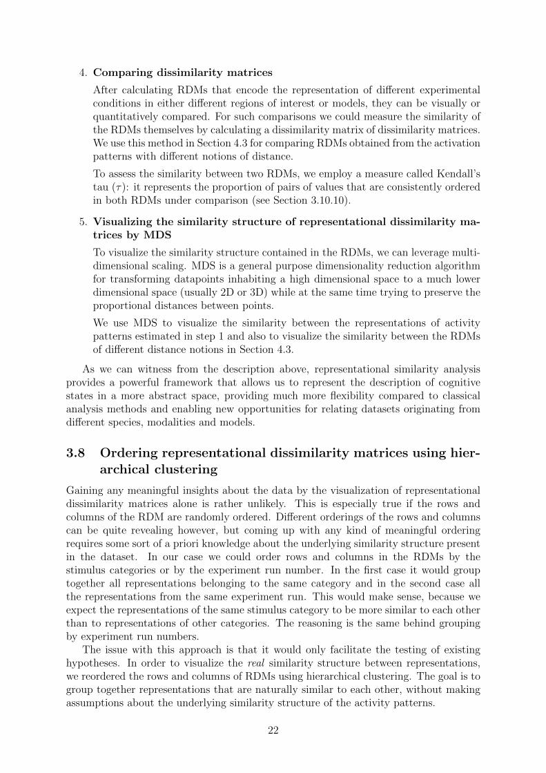
Just for comparison, the same RDM is shown on Figure 10, but there the rows andcolumns are randomly ordered. Clearly we can get more intuition about the underlyingsimilarity structure between the stimulus categories from the visualization in Figure 9.We can immediately observe that small objects like shoes, bottles and scissors seem tohave more similar representations than objects from other categories. This observationis not obvious by looking at Figure 10.

3.9 Dimensionality reduction using multidimensional scaling

Although we showed in Section 3.8 that representational dissimilarity matrices can betransformed to visualize the information they contain in a more meaningful way, they arein general not the best tool for visualizing the similarity structure between representationsof cognitive states. A more useful technique for creating this kind of visualization is calledmultidimensional scaling. MDS is a general dimensionality reduction technique first pro-posed by Joseph Kruskal in a 1964 paper [Kru64]. Since then multiple variations of thisclassical version have been developed [BG05]. In this thesis we used the MDS implemen-tation provided by the Scikit-Learn machine learning toolkit exclusively [PVG+11].

In general MDS is used to reduce the dimensionality of datapoints residing in a highdimensional space and project these points into a space of much lower dimensions. Thereal utility of MDS lies in the fact that this projection is carried out in such a waythat distances between the points in the high dimensional space are preserved as much aspossible in the lower dimensional space. The dimensionality of the space to project pointsonto is usually chosen to be either two or three dimensions to facilitate visualization.

We use MDS extensively to construct 2D scatterplots in order to visualize the sim-ilarity between representations of different stimulus categories in the brain. The repre-sentations are activation patterns consisting of voxel intensities and their dimensionality

23

Figure 9: Representational dissimilarity matrix for the stimulus categories as calculatedusing the Mahalanobis distance. The rows and columns are ordered based on the orderingof the leaf nodes in the dendrogram resulting from hierarchical clustering.

24

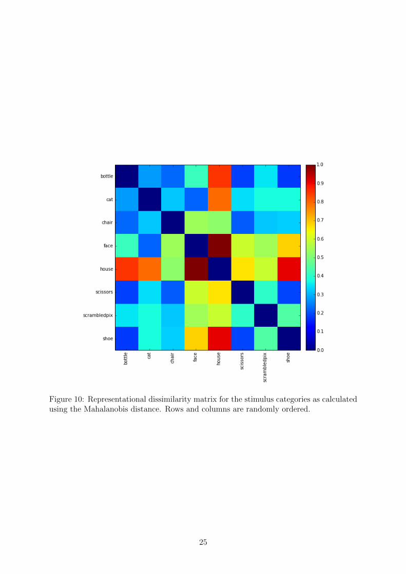
Figure 10: Representational dissimilarity matrix for the stimulus categories as calculatedusing the Mahalanobis distance. Rows and columns are randomly ordered.

25

is defined by the region of interest. Since the region of interest used in this thesis (theventral temporal cortex 3.5) is the size of about 500 voxels in our scan data, we essen-tially perform dimensionality reduction using MDS from a 500-dimensional space into a2-dimensional space. The distances between activation patterns, that MDS operates on,are defined by the representational dissimilarity matrix calculated during the process ofrepresentational similarity analysis.

3.10 Different notions of distance

This section presents the description of all the different notions of distance evaluatedin this thesis. Almost all of the distance measures presented here are defined betweentwo vectors u and v. These two vectors represent the activity patterns in our fMRIdata, elicited by different stimulus categories. The vectors are of length n, which is thenumber of voxels in the particular region of interest the vectors were obtained from.The individual components of the vectors ui and vi are the voxels intensity values. Thedescriptions were obtained from [Cha07] and are presented in alphabetical order.

3.10.1 Bray-Curtis distance

n∑i=1

|ui − vi|n∑

i=1

(ui + vi)

(3)

3.10.2 Canberra distancen∑

i=1

|ui − vi|ui + vi

(4)

3.10.3 Chebyshev distance

maxi|ui − vi| (5)

3.10.4 Cityblock distance

n∑i=1

|ui − vi| (6)

3.10.5 Correlation distancen∑

i=1

(ui − u)(vi − v)√√√√ n∑i=1

(ui − u)2n∑

i=1

(vi − v)2(7)

Where u and v are the means of vectors u and v respectively.

26

3.10.6 Cosine distanceu · v√√√√ n∑

i=1

u2i

√√√√ n∑i=1

v2i

(8)

Where u · v is the dot product between vectors u and v.

3.10.7 Euclidean distance √√√√ n∑i=1

(ui − vi)2 (9)

3.10.8 Hamming distance

The Hamming distance between two vectors is defined as the proportion of componentsthat differ between the vectors:

n∑i=1

I(ui, vi)

n(10)

where I is a function returning 0 if ui = vi and 1 otherwise.

3.10.9 Mahalanobis distance

While most of the metrics presented in this thesis measure the similarity between twovectors, the Mahalanobis distance measures the similarity between two groups of ob-jects [DMJRM00]. In our case this means the overall similarity between all the represen-tations of stimuli from different categories (not between two single instances of activitypatterns representing stimuli from different categories). We will call this concept similar-ity between categories.

For starters let us define the mean elements for two different stimulus categories asu and v. These are obtained by averaging all the individual activity patterns for aparticular stimulus category component-wize. Essentially u and v represent the averageactivity patterns for two different stimulus categories. The Mahalanobis distance usingthese is defined as: √

(u− v)TS−1(u− v) (11)

Here S−1 is the inverse of the pooled covariance matrix for the two categories:

S =cov(U) + cov(V)

2(12)

U and V are matrices containing all the activity patterns from the two differentstimulus categories under consideration.

3.10.10 Kendall’s tau

This metric is used for the comparison of two representational dissimilarity matricesin this thesis. It essentially describes the correlation (or more specifically agreementof the ordering of values) between the two RDMs, but in a way that is different fromSpearman correlation for example. It was chosen on the basis that it was the suggested

27

measure for comparing RDMs in a recent review article on representational similartyanalysis [NWW+14b]. In this thesis we use the implementation of Kendall’s τ providedby the SciPy (Open source scientific tools for Python) package [JOP14]. Their manualdescribes Kendall’s τ between two rankings X and Y (the RDMs in our case) as:

P −Q√(P +Q+ T )(P +Q+ U)

(13)

where P is the number of concordant pairs, Q the number of discordant pairs, T thenumber of ties only in X, and U the number of ties only in Y. If a tie occurs for thesame pair in both X and Y, it is not added to either T or U.

28

4 Results

This chapter summarizes all the results from the research carried out for this thesis.It starts by presenting the results from classification analysis described in Section 3.6,followed by a thorough example of the representational analysis pipeline used throughoutthis chapter. Then results from the comparison of different distance notions described in3.10 are shown, together with their interpretation. Finally we finish off this chapter byintroducing a novel use case for RSA as a technique for exploratory data analysis.

4.1 Validating the region of interest

Since the results of representational similarity analysis for a specific region of interest inthe brain are not always straightforward to interpret, it would good to have a methodfor validating the ROI beforehand. By validation we want to determine if we can expectmeaningful results from a ROI in the first place.

Since we would like to know how are objects belonging to different categories repre-sented in different parts of the brain, the obvious starting point would be to check howwell we can separate the samples in our dataset with respect to the categories.

To verify the fact that our ROI does indeed contain the necessary information todistinguish between different stimulus categories in the experiment, we trained a linearSVM classifier using data from only this region. The training procedure used fMRIactivation patterns from all the experiment runs of a single subject and also included anN-fold cross-validation procedure (for a detailed description see Section 3.6). As a resultof this analysis we obtained an average classification accuracy of 0.81 across all subjects.This was calculated by averaging the results across all the folds for a single subject.Clearly the accuracy is well above chance level for eight different categories (0.125) andshows that our region of interest definitely contains information about the categories ofdifferent stimuli presented to the subjects.

Figure 11 shows the classifier accuracy for a single subject represented as a confusionmatrix. The confusion matrix helps us visualize classification accuracy for the differentactivation patterns by category and helps us identify the categories where instances aremislabeled more often. The strong diagonal in Figure 11 is an indication of a good overallclassification accuracy. The categories with the highest identification accuracy are faces,houses, scrambled pictures, cats and chairs while small objects like bottles, scissors andshoes are mislabeled more often. Our results are in direct correlation with the resultsobtained by Haxby et al. [HGF+01] for the same dataset.

29

Figure 11: Confusion matrix of classifier results for subject 1. The color represents theproportion of instances for each category.

4.2 Classical representational similarity analysis

After validating our region of interest for the necessary information, we proceed to carryout classical representational similarity analysis on data from this brain region. All thesteps implemented here are described in full detail in Section 3.7 together with reasoningbehind each step. In this section we only describe the inputs for each step and makesome remarks about the results. The analysis implemented here will serve as a templatefor the following sections where we run the same analysis, but with different notions ofdistance.

For step one we estimated the activity patterns that represent our experimental condi-tions, each pattern represents one of the eight categories for a stimulus image. Altogetherwe have 96 of these activity patterns each consisting of 577 voxels.

Next we calculate the Euclidean distance between each pair of activity patterns andassemble the results into a representational dissimilarity matrix, shown on Figure 12. Thematrix is symmetrical around a diagonal of zeroes (the distance between each activitypattern and itself is zero) and is ordered by stimulus category, grouping together activitypatterns elicited by stimuli belonging to the same category.

Visualizing the RDM as in Figure 12 is not very informative by itself. We can witnesssome distinctive square patterns formed mostly around the diagonal for some categories(indicating a close similarity between all the activity patterns comprising these particularcategories) and we can also observe that some activity patterns are very dissimilar to all

30

Figure 12: 96 x 96 Representational dissimilarity matrix. Represents the similarity struc-ture between each pair of 96 different activity patterns (grouped by the stimulus categorythat ellicited them). Distance values are scaled to be between 0 and 1, the latter repre-senting the maximum distance calculated between any two representations.

31

other activity patterns not belonging to their particular category. Still this does not giveus a clear way to visualize the relation of representations of different stimulus categories.

To try to visualize the relationship between representations of different stimulus cat-egories more clearly, we reordered the rows and columns of the representational dissim-ilarity matrix. The new ordering was generated by clustering the distances of activitypatterns in the RDM using hierarchical clustering. This process is described in moredetail in Section3.8. The output of hierarchical clustering is a dendrogram where the leafnodes are our activity patterns and they are ordered based on their similarity. We usedthis ordering for the rows and columns of the dissimilarity matrix. The main idea forthis sort of reordering of the RDM is to visualize ”natural” clusters of activity patternsin the dataset. The results are shown on Figure 13.

Figure 13: Representational dissimilarity matrix with rows and columns reordered toplace similar activity patterns together.

In this new matrix we see more distinctive rectangular patterns and not all of themare around the diagonal anymore either. This is a clear indication that our dataset con-tains some structure with respect to our chosen distance metric (the Euclidean distance).We would expect that representations of activity patterns caused by the same stimulus

32

category would be close together, but as we see from Figure 13 this is not always thecase. Although there is some clustering in that respect, like houses, the overall similaritystructure seems to be more complex.

The third step in our analysis involves the creation of a model. For this we chose aconceptual model inspired by one described in [KMB08]. Our model describes a hypo-thetical region of the brain where representations of animate and inanimate objects arevery dissimilar. If we presented our model with the exact same stimuli as were presentedto the subjects in the experiment and carried out the first two steps of RSA, the resultingRDM from the model would look like the one depicted on Figure 14.

Figure 14: Representational dissimilarity matrix from a model distinguishing perfectlybetween animate and inanimate objects.

The RDM from the model depicts representations of stimulus categories of animateobjects (cats and faces) being maximally similar to each other while at the same timemaximally dissimilar to representations of inanimate objects (bottles, chairs, houses,scissors, scrambled pictures and shoes). This model is of course very simplistic as itdoes not model any noise or other variables except our conceptual notion of animateand inanimate objects being very distinguishable. In fact we do not have any reasonable

33

neuroscientific justification for believing that our experimental region of interest (theventral temporal cortex) is able to distinguish between animate and inanimate objectsat all. Still for the purposes of this thesis, the model will serve well for comparison withRDMs based on actual activity patterns as our goal is not to prove the validity of thismodel for the experimental region of interest.

The Kendall’s τ coefficient between the RDM on Figure 12 and our model is 0.16.The interpretation behind this is that the correlation between representations of cognitivestates within the model and actual measured activity patterns is very weak. This impliesthat the actual information processing occurring in the ROI interest under study is verydifferent from the assumptions of our simplified model (as was expected) and that thisparticular area in the brain does not make a very clearly identifiable distinction betweenanimate and inanimate objects.

For the final step we visualize the similarity structure of the representations of cog-nitive states contained in the RDMs by multidimensional scaling. Figure 15 shows twoplots, both based on the RDM in Figure 12. The distances of individual points in theplots represent the actual distances of the different neural representations (voxel acti-vation patterns) for each experiment block (as measured by Euclidean distance). Themotivation behinds using two plots instead of one, is to both visualize the variance insimilarity between representations of the same stimulus category and the distance be-tween representations of different categories more clearly at the same time.

Figure 15: Multidimensional scaling of the representations of cognitive states ellicited bythe stimulus images. On the left: each dot is the neural representation of a stimulusblock in the experiment (the representation of the category of a stimulus). On the right:centroids for the individual points in the left plot averaged by category.

From Figure 15 we can gather that representations of houses and faces seem to exhibita relative high within category similarity between instances (tighter grouping), while therepresentations of smaller objects like shoes, bottles and scissors have a not so clearlydefined similarity structure and are therefore more difficult to distinguish, as individualrepresentations from these categories are intermingled with each other. Although the re-sults are not directly comparable, intuitively we could argue that they coincide somewhatwith the results of the classifier analysis implemented in Section 4.1, where small objectswere mislabeled more often, while houses and faces had a much higher accuracy.

34

For visual comparisons we also ran MDS on our model that distinguishes only betweenanimate and inanimate objects, the results are shown on Figure 16.

Figure 16: MDS results from a conceptual model distinguishing perfectly between animateand inanimate objects.

Purely by visual comparison we are able to draw additional verification for the lowKendall coefficient calculated earlier. As in the model we see the centroids for the facesand cats category very close together and at the same time very far apart from all therest of the categories, while in the plots of the actual representations, we cannot reallysay that cats are more closer to faces than for example bottles or shoes.

35

4.3 The effect of distance on RSA

The main goal of this thesis is to study different notions of distance between the activitypatterns measured in the subjects and the effect they have in the context of representa-tional similarity analysis. This section summarizes the results we obtained by comparing9 different distance notions (described in Section 3.10).

In order to compare the effects of different distance functions, we first carried outRSA as described in Section 4.2 substituting the Euclidean distance used in that sectionwith all the different notions of distance in turn. The results from multidimensionalscaling for each different notion of distance are shown on Figures 17 - 24, visualizing foreach distance the similarity structure between representations of all the different stimulusblocks on the left and the similarity between stimulus categories on the right. The rightplots visualize the centroids of individual points on the left by category.

The multidimensional scaling plots are useful to visualize general tendencies in thedata and how stable these tendencies are in the face of changing distance functions. Asthe whole idea of RSA is to abstract away from individual activation patterns, we wouldlike to know if the distance functions used to estimate the representational similaritystructures of activity patterns have any effect on this higher level of abstraction. For thiswe compared the RDMs constructed with different distance functions to the RDM of ouranimate-inanimate model via the Kendall’s τ coefficient (Table 1).

Figure 17: MDS results using Bray-Curtis distance

Some distinctive patterns emerge from the plots on Figures 17 - 24. For almost alldifferent distance notions, representations from the ”face” and ”house” categories exhibitthe greatest within category similarity (tight grouping on most of the plots). Repre-sentations from all the other categories do not exhibit such a clearly defined similaritystructure within their category. Representations of faces and houses are also consistentlymost dissimilar to each other as indicated by the centroid plots on the right. Some dis-tance notions like Chebyshev and Correlation distance seem to exhibit a tighter groupingalso in the ”cat” category, but the results are far from conclusive.

Both the MDS plots and model correlation coefficients on Table 1 show Hammingdistance as the odd ball out. Recall from Section 3.10 that Hamming distance between twovectors represents the proportion of those vector elements between the two n-dimensional

36

Figure 18: MDS results using Canberra distance

Figure 19: MDS results using Chebyshev distance

Table 1: Comparison of activity pattern RDMs to the model RDMDistance notion Kendall’s τ coefficientBray-Curtis 0.22Canberra 0.21Chebyshev 0.18Cityblock 0.16Correlation 0.22Cosine 0.25Euclidean 0.17Hamming 0.08Mahalanobis 0.34

37

Figure 20: MDS results using Cityblock distance

Figure 21: MDS results using Correlation distance

38

Figure 22: MDS results using cosine distance

Figure 23: MDS results using Hamming distance

39

vectors u and v which disagree. As such it is only meant to be used for vectors of discreteelements. Since our fMRI image vectors contain continuous values, it really makes nosense whatsoever in using the Hamming distance to assess the similarity between them.In fact the only reason Hamming distance was added to this comparison in the firstplace, was to serve as an example that not all distance metrics between any two vectorsare appropriate in the domain of fMRI data analysis. Adding such a nonsensical metricin this context can also serve as a sort of additional validation of the analysis pipeline inthe sense of determining how easily we can detect the uselessness of this metric from theresults.

As for the comparison with the model, when we look at Table 1 (excluding the Ham-ming distance), indeed there exist some differences in the correlation between the differentRDMs and the model RDM. Especially representations estimated using the Mahalanobisdistance do seem to correlate more with the model than representations from any otherdistance notion. This might have something to do with the way we generated the RDMfor Mahalanobis distance. Since the Mahalanobis distance metric measures the similar-ity between stimulus categories not between the representations of individual stimulusblocks as all the other metrics, we had to interpolate the RDM for Mahalanobis distancein order to compare it with the model. As the model RDM is a 96 x 96 matrix andthe initial result from Mahalanobis was a 8 x 8 matrix (similarity between each of the 8categories), we used nearest neighbor interpolation to construct a 96 x 96 matrix fromthe original 8 x 8 matrix. This essentially means that all the individual representationsin the interpolated matrix for a single category are identical and represent the average ofall the individual samples in some sense.

For a better comparison of the results from multidimensional scaling, we calculated the

Figure 24: MDS results using Mahalanobis distance

40

pairwise distances of all the centroids from the right plots and ordered them by distancefrom smallest to largest. Since in essence the distances between centroids represent theaverage similarity between stimuli from different categories, we wanted to see how thisranking of pairwise distances changed with respect to the distance notion used. Thisdifference in the rankings is visualized on Figure 25. Since this visualization is justanother technique for representing the results from all the MDS plots in a more conciseway, we can draw the exact same conclusions as before. The overall tendencies for allthe different distance notions are largely the same - the distance between faces andhouses is the greatest with all the meaningful distance functions used, while there arealso considerable similarities in the pairwise distances for the small objects. Neverthelessthere are specific differences, for example the distance between scrambled pictures andfaces is estimated very differently between the Euclidean distance (13th in the ranking)and a group consisting of cosine, Canberra and Bray-Curtis distances (second largestdistance).

Figure 25: The ranking of pairwise distances between average representations of differentstimulus categories for each notion of distance used. The pairs of categories are orderedand colored according to their ranking in the Euclidean distance, from smallest pair-wise distance (purple) to largest pairwise distance (red). This allows us to visualize thedifferences of ranking, by taking Euclidean distance as a reference

For a final comparison of the different distance functions, we calculated the secondorder similarity between their results (the similarity between each pair of RDMs which inturn represent the similarity structures estimated from the underlying activity patternswith different notions of distance). Figure 26 depicts the relative similarity of the differentdistance notions under consideration.

41

Figure 26: MDS visualization of second order similarity between all the RDMs calculatedwith different distance notions. 1 − Kendall′sτ is used to calculate the dissimilaritybetween RDMs.

42

4.4 RSA as a tool for assessing data quality

While doing research for this thesis and analysis tests, we ended up visualizing many dif-ferent configurations of representational distance matrices and multidimensional scalingplots. This constant visual feedback led us to discover a bug in our data preprocessingpipeline which would have been very difficult to detect by other means. Therefore wepropose the notion that several steps from the representational similarity analysis pipelinecould also be used for assessing the effects of different data preprocessing techniques andother transformations.

Our dataset is a timeseries of fMRI volumes each consisting of hundreds of voxelsrecorded at different timepoints. When dealing with multivariate data such as this, itcan be very difficult to visualize what effect a particular transformation (like detrending)has on the dataset as a whole. Possibilities include visualizing raw voxel intensities, whichis not very informative. Another sometimes useful technique is to visualize the timeseriesof one or a couple of individual voxels, but still this is lacking a global point of view.Combine these problems with the inherently low signal to noise ratio of fMRI data andthe situation looks pretty bleak.

It turns out that we can actually leverage RSA to help alleviate the lack of globallyeffective visualization options. Since RSA handles the individual data samples (fMRIvolumes) on a more abstract level, we are able to observe changes caused by transforma-tions of the original samples in a more meaningful way. As an example consider the tworepresetational dissimilarity matrices on Figure 27.

Figure 27: Two RDMs representing the similarity structure between individual fMRIvolumes of the ”faces” category.

They both represent the similarity structure of individual fMRI volumes from only the”faces” category. Our underlying assumption here is that since the representations arecaused by the same stimulus category, they should be pretty similar to each other. Thedistinguishing block texture we can observe on them stems from the fact that samples arerecorded on different experiment runs and recordings from on different runs are boundto be more dissimilar. Still we notice that even samples from the same run show up asbeing very dissimilar in the left RDM. This led us to believe that some of the samples inthe dataset vere mislabeled, which upon the revising of our preprocessing pipeline turned

43

out to be correct. The right RDM represents the same data, but with correct processingof the labels of individual fMRI volumes.

This example also illustrates the fact that it can be beneficial at times to visualizeonly slices from the entire RDM to focus on specific questions related to only some ofthe conditions. Visualizing the entire RDM can be useful for detecting areas that can beinteresting for more detailed study.

Altough we did validate our data with a classification analysis (Section 4.1), even withthe mislabeled samples, the average classification accuracy was way beyond chance level.The implication here are that by relying on the accuracy metric alone, this discoverywould never have been made. With the corrected pipeline, we managed to improveclassification accuracy by another 12%.

The above is just one example of how RSA can be leveraged to provide a view intothe data from a different angle. This is somewhat analogous to how a Fourier transformis used in signal processing to convert a time domain signal into frequency domain, inorder to study different aspects of the same signal [Bra65]. We think that RSA can alsobe used to visualize the effects of other preprocessing steps like detrending, normalizationand z-scoring.

44

5 Discussion

As far as we know, we are the first to conduct a systematic study into the effects of differ-ent distance notions in the context of representational similarity analysis. Most literatureabout RSA seems to prefer the use of Correlation distance to assess the similarity betweenactivation patterns ([KMB08], [KMR+08]), because it normalizes for both the mean levelof activity and the variability in the activation patterns. Although there is also mention-ing of Euclidean and Mahalanobis distances in the context of RSA ( [NWW+14a]), wehave not seen any thorough comparisons between them.

As we evaluated 9 different notions of distance, we did so with no particular neuro-scientific research question to optimize for. In other words, we were not trying to findthe ”best” notion of distance, as the utility of a particular distance measure would onlybecome apparent in the context of some specific research goals. An example of this wouldbe a study where in addition to the neural representations, the reaction times of a subjectfor experimental stimuli would also be recorded. In this case RSA could be used to relatethe neural representations of specific stimuli to the reaction times corresponding to thosesame stimuli. Here a useful metric would be one that maximises the correlation betweenthe neural representations and the reaction times. Since we did not have a dataset withsuch behavioral data at hand, we evaluated the distance measures against a conceptualmodel instead.

We showed that although there are differences in the final results of RSA dependingon the distance measure used to estimate the similarity between initial activity patterns,the differences in our case did not change the most prevalent trends in the results - allthe distance measures exhibited noticeable grouping for the representations of housesand faces. What is more interesting however is that there exist considerable similari-ties between some distance notions. For example the Bray-Curtis, Canberra and Cosinemeasures produce different but very similar pairwise distance rankings of the representa-tions of stimuli. The same can be said for Euclidean and Cityblock distances, which areeven more similar. Being aware of this kind of grouping among the measures can saveresearchers some time when they are evaluating different distance notions for a particularuse case. They can then only focus on measures that are from different groups. Based onour results the optimal set of distances to evaluate for a research problem would containMahalanobis, Correlation, Euclidean, Chebyshev and Cosine metrics.

This kind of grouping of measures demonstrated by our analysis is not surprisinghowever. From a mathematical perspective, the notions of distance are not fully inde-pendent and one could have expected similar behavior for a few of them as indicated bythe grouping. As we implemented only experimental comparisons of the distance mea-sures, we refer the reader to a general overview paper where the semantic and syntacticsimilarity is also taken into account when doing comparisons [Cha07].

Next we will propose some additional ideas and variations to the techniques used inthis thesis for further research in the future:

• In Section 4.4 we presented another use case for RSA as a tool to visualize theeffects different transformations on the input dataset have on a global level. Wepostulated that RSA might be useful to assess the effects different preprocessingsteps like detrending, intensity normalization or z-scoring have on the data visually.Another direction would be to try to automate the process for finding optimalpreprocessing steps. We could try different ranks of polynomials for the detrendingprocess, carry out RSA for each of them and define some metric to assess the quality

45

of the resulting RDMs (for example the average similarity between representationsof the same category). This is a tricky proposition, as we know now that the resultswould depend not only on the metric defined for the RDMs, but also from the notionof distance used to estimate the similarity between activity patterns themselves.

• The list of notions evaluated for this thesis is by no means comprehensive. Wetried to select a good subset of known distance measures and the main goal was toshow whether they have any difference at all in the context of RSA. The obvioussuggestion here would be to continue the research with more distance measures.It would be especially interesting to see how modality specific distance measurescompared with our results. By that we mean measures that are specifically adaptedto take into account also the spacial structure of fMRI images for example. A setof such novel measures is proposed by Novatnack et al. [NCS+08].

• All analysis in this thesis was carried out on data coming only from a single subject.Since the dataset contained the neural responses for six different subjects, compar-isons could be made by carrying out the same analysis for different subjects.

• We described the concept of defining a region of interest in the brain functionallyin Section 3.5. One possible area of interest would be to use some functionallydefined regions in determining if there are some regions where the overall similaritiesbetween distances as illustrated on Figure 26 differ significantly.

• Multidimensional scaling is extensively used in this thesis to visualize similaritystructures contained in representational similarity matrices. In a review articleon RSA [NWW+14b] another method besides MDS is also suggested for the samepurpose, called t-SNE [VdMH08]. We actually evaluated t-SNE for visualizing thedistances between representations in this thesis. In some cases it would yield moreaesthetically pleasing results than MDS, but that required careful tuning of theinput parameters. MDS was chosen over t-SNE mainly because the results weobtained with the latter were inconclusive. Still t-SNE could prove to be a viablealternative for MDS, but this needs more research.

46

6 Conclusions

In this thesis we presented a thorough overview of how to implement representationalsimilarity analysis on fMRI data using a well known dataset in neuroscience as the basis.We demonstrated all the steps in a typical RSA pipeline starting from the preprocessingof data and ending with the interpretation of the results. We also showed how thevisualizations of representational dissimilarity matrices can be improved by hierarchicalclustering.

The main goal of this thesis was to evaluate 9 different notions of distance to be usedfor estimating the similarity between representations of different stimuli in the brain andthe effect these distance notions have on the overall result of RSA. We concluded that theresults of RSA indeed differ with respect to the distance measures used between activitypatterns and that there exist considerable similarities between different groups of distancemeasures.

In addition to the comparison of distance metrics, we also proposed a novel use casefor representational similarity analysis as a tool for visualizing the effects of differenttransformations on the input data on a global level.

47

References

[AB06] Edson Amaro and Gareth J Barker. Study design in fmri: basic principles.Brain and cognition, 60(3):220–232, 2006.

[BG05] Ingwer Borg and Patrick JF Groenen. Modern multidimensional scaling:Theory and applications. Springer Science & Business Media, 2005.

[Bra65] Ron Bracewell. The fourier transform and iis applications. New York, 1965.

[CAB+04] Robert W Cox, John Ashburner, Hester Breman, Kate Fissell, ChristianHaselgrove, Colin J Holmes, Jack L Lancaster, David E Rex, Stephen MSmith, Jeffrey B Woodward, et al. A (sort of) new image data formatstandard: Nifti-1. Human Brain Mapping, 25:33, 2004.

[Cha07] Sung-Hyuk Cha. Comprehensive survey on distance/similarity measuresbetween probability density functions. City, 1(2):1, 2007.

[Dev07] H Devlin. What is functional magnetic resonance imaging(fmri)? Psych Central, 2007. http://psychcentral.com/lib/

what-is-functional-magnetic-resonance-imaging-fmri/0001056.

[DMJRM00] Roy De Maesschalck, Delphine Jouan-Rimbaud, and Desire L Massart. Themahalanobis distance. Chemometrics and intelligent laboratory systems,50(1):1–18, 2000.

[EZB13] Joset A Etzel, Jeffrey M Zacks, and Todd S Braver. Searchlight analysis:promise, pitfalls, and potential. Neuroimage, 78:261–269, 2013.

[Gre07] Michael Greenacre. Correspondence analysis in practice. CRC Press, 2007.

[HDO+98] Marti A. Hearst, Susan T Dumais, Edgar Osman, John Platt, and Bern-hard Scholkopf. Support vector machines. Intelligent Systems and theirApplications, IEEE, 13(4):18–28, 1998.

[HGF+01] James V Haxby, M Ida Gobbini, Maura L Furey, Alumit Ishai, Jennifer LSchouten, and Pietro Pietrini. Distributed and overlapping representationsof faces and objects in ventral temporal cortex. Science, 293(5539):2425–2430, 2001.

[HHS+09] Michael Hanke, Yaroslav O Halchenko, Per B Sederberg, Stephen Jose Han-son, James V Haxby, and Stefan Pollmann. Pymvpa: A python toolbox formultivariate pattern analysis of fmri data. Neuroinformatics, 7(1):37–53,2009.

[HMH04] Stephen Jose Hanson, Toshihiko Matsuka, and James V Haxby. Combina-torial codes in ventral temporal lobe for object recognition: Haxby (2001)revisited: is there a “face” area? Neuroimage, 23(1):156–166, 2004.

[JOP14] Eric Jones, Travis Oliphant, and Pearu Peterson. {SciPy}: Open sourcescientific tools for {Python}. 2014.

48

[KB07] Nikolaus Kriegeskorte and Peter Bandettini. Analyzing for information,not activation, to exploit high-resolution fmri. Neuroimage, 38(4):649–662,2007.

[KK13] Nikolaus Kriegeskorte and Rogier A Kievit. Representational geometry:integrating cognition, computation, and the brain. Trends in cognitive sci-ences, 17(8):401–412, 2013.

[KMB08] Nikolaus Kriegeskorte, Marieke Mur, and Peter Bandettini. Representa-tional similarity analysis–connecting the branches of systems neuroscience.Frontiers in systems neuroscience, 2, 2008.

[KMR+08] Nikolaus Kriegeskorte, Marieke Mur, Douglas A Ruff, Roozbeh Kiani, JerzyBodurka, Hossein Esteky, Keiji Tanaka, and Peter A Bandettini. Matchingcategorical object representations in inferior temporal cortex of man andmonkey. Neuron, 60(6):1126–1141, 2008.

[Kru64] Joseph B Kruskal. Multidimensional scaling by optimizing goodness of fitto a nonmetric hypothesis. Psychometrika, 29(1):1–27, 1964.

[Log03] Nikos K Logothetis. The underpinnings of the bold functional magneticresonance imaging signal. The Journal of Neuroscience, 23(10):3963–3971,2003.

[NCS+08] John Novatnack, Nicu Cornea, Ali Shokoufandeh, Deborah Silver, SvenDickinson, Paul Kantor, and Bing Bai. A generalized family of fixed-radiusdistribution-based distance measures for content-based fmri image retrieval.Pattern Recognition Letters, 29(12):1726–1732, 2008.

[NPDH06] Kenneth A Norman, Sean M Polyn, Greg J Detre, and James V Haxby.Beyond mind-reading: multi-voxel pattern analysis of fmri data. Trends incognitive sciences, 10(9):424–430, 2006.

[NWW+14a] Hamed Nili, Cai Wingfield, Alexander Walther, Li Su, William Marslen-Wilson, and Nikolaus Kriegeskorte. A toolbox for representational similar-ity analysis. PLoS computational biology, 10(4):e1003553, 2014.

[NWW+14b] Hamed Nili, Cai Wingfield, Alexander Walther, Li Su, William Marslen-Wilson, and Nikolaus Kriegeskorte. A toolbox for representational similar-ity analysis. PLoS computational biology, 10(4):e1003553, 2014.

[OJAH05] A O’toole, Fang Jiang, Herve Abdi, and J Haxby. Partially distributedrepresentations of objects and faces in ventral temporal cortex. CognitiveNeuroscience, Journal of, 17(4):580–590, 2005.

[PBM+13] Russell A Poldrack, Deanna M Barch, Jason P Mitchell, Tor D Wager,Anthony D Wagner, Joseph T Devlin, Chad Cumba, Oluwasanmi Koyejo,and Michael P Milham. Toward open sharing of task-based fmri data: theopenfmri project. Frontiers in neuroinformatics, 7, 2013.

[PG07] Fernando Perez and Brian E. Granger. IPython: a system for interactivescientific computing. Computing in Science and Engineering, 9(3):21–29,May 2007.

49

[PMB09] Francisco Pereira, Tom Mitchell, and Matthew Botvinick. Machine learningclassifiers and fmri: a tutorial overview. Neuroimage, 45(1):S199–S209,2009.

[PPFR88] Michael I Posner, Steven E Petersen, Peter T Fox, and Marcus ERaichle. Localization of cognitive operations in the human brain. Science,240(4859):1627–1631, 1988.

[PVG+11] Fabian Pedregosa, Gael Varoquaux, Alexandre Gramfort, Vincent Michel,Bertrand Thirion, Olivier Grisel, Mathieu Blondel, Peter Prettenhofer, RonWeiss, Vincent Dubourg, et al. Scikit-learn: Machine learning in python.The Journal of Machine Learning Research, 12:2825–2830, 2011.

[RKB12] C Rorden, HO Karnath, and L Bonilha. Mricron dicom to nifti converter.Neuroimaging Informatics Tools and Resources Clearinghouse (NITRC),2012.

[Slo13] Guy Slowik. What is magnetic resonance imaging (mri)?, 2013. http:

//ehealthmd.com/content/what-magnetic-resonance-imaging-mri.

[Str06] Stephen C Strother. Evaluating fmri preprocessing pipelines. Engineeringin Medicine and Biology Magazine, IEEE, 25(2):27–41, 2006.

[TMT+02] Jody Tanabe, David Miller, Jason Tregellas, Robert Freedman, and Fran-cois G Meyer. Comparison of detrending methods for optimal fmri prepro-cessing. NeuroImage, 15(4):902–907, 2002.

[VdMH08] Laurens Van der Maaten and Geoffrey Hinton. Visualizing data using t-sne.Journal of Machine Learning Research, 9(2579-2605):85, 2008.

[VRN+11] Vincent Q Vu, Pradeep Ravikumar, Thomas Naselaris, Kendrick N Kay,Jack L Gallant, and Bin Yu. Encoding and decoding v1 fmri responses tonatural images with sparse nonparametric models. The annals of appliedstatistics, 5(2B):1159, 2011.

50

Non-exclusive licence to reproduce thesis and make thesis public

I, Martin Loginov (date of birth: 14th of July 1987),

1. herewith grant the University of Tartu a free permit (non-exclusive licence) to:

1.1 reproduce, for the purpose of preservation and making available to the public,including for addition to the DSpace digital archives until expiry of the term ofvalidity of the copyright, and

1.2 make available to the public via the web environment of the University ofTartu, including via the DSpace digital archives until expiry of the term ofvalidity of the copyright,

Beyond decoding: representational similarity analysis on fMRI data

supervised by Raul Vicente Zafra

2. I am aware of the fact that the author retains these rights.

3. I certify that granting the non-exclusive licence does not infringe the intellectualproperty rights or rights arising from the Personal Data Protection Act.

Tartu, 20.05.2015

51