Embed Size (px)
Citation preview

1
VIII-4 Hydrologic Systems Risk
Best Practices in Dam and Levee Safety Risk Analysis
26 February 2015
2
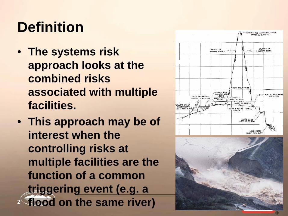
Definition • The systems risk
approach looks at the combined risks associated with multiple facilities.
• This approach may be of interest when the controlling risks at multiple facilities are the function of a common triggering event (e.g. a flood on the same river)

3
Applicability
• Corrective action studies involving hydrologic PFMs whose estimated risks are tied to the ability to pass or not pass a flood (i.e. overtopping PFMs)
• Note that the decision to move to corrective action would be based on the risks associated with an individual facility

4
Basic Motivation
• To develop a more cost effective fix for the facility that is the primary focus of the corrective action study by distributing some of the modification work (and on paper, some of the risk) to other dams in the system
• To lower the overall risk associated with the system of dams

5
Is this something I can do?
• The team must have a working understanding of basic probability theory concepts (ME and CE events, intersection probability, conditional probability, Venn diagram)
• For higher level studies, the expertise of a hydrologist or loadings specialist may be needed

6
Individual versus system risks • For an individual facility, the
risk is estimated in terms of potential failure modes. The PFMs are often treated as ME events or transformed via the common cause adjustment (CCA)
• For ME PFMs, the occurrence probabilities of the individual PFMs (the AFPs) can be summed to obtain the total probability of dam failure

7
Individual versus system risks • In the hydrologic systems
approach, the “PFMs” of the system are the individual dam failure events (e.g. “Dam A fails”, “Dam B fails”)
• Unlike in the case of the individual dam approach, these “PFMs” are not considered to be ME, and the probability of the intersection event cannot be ignored

8
Individual versus system risks • Considered individually, a
pair of dams has a total of two fail outcomes, A (Dam A fails) and B (Dam B fails). In contrast, a system of two dams has three fail outcomes
• Note that the system failure probability is not equal to the sum of the probabilities of the individual-dam fail outcomes
)BP(AP(AB)B)AP()P(FailSYS ++=P(B)P(A))P(FailSYS +≠

9
Precedence and causality • Consider a pair of dams A
and B, with Dam A located upstream of B. All major floods are thought to originate upstream of A
• Note that whereas the Venn diagram intersection event AB describes the failure of both dams, the occurrence of the AB event does not imply that upstream dam fails 1st

10
Precedence and causality • In contrast, the following event tree assumes
that if both dams fail, A fails first • Can lead to confusion if the Dam B individual-
dam risk estimates are not premised on non-failure of A
Flood Loadings (PFL)
Dam A - Fails
Dam B - Fails
Dam B - Fails
Dam A – Non-Failure
Dam B – Non-Failure
Dam B – Non-Failure
PA
1-PA
PB|A
1-PB|A
PB|Ā
1- PB|Ā
Response to hydrographs (Dam A inflow)
Response to hydrographs (Dam A breach outflow)
Response to hydrographs (Dam A outflow + intervening flows)
A|BAFL xPxPPP(AB) =
( )A|BAFL P-1xxPP)BP(A =
( ) A|BAFL xPP-1xPB)AP( =
( ) ( )A|BAFL P-1xP-1xP)BAP( =

11
Precedence and causality • In order to help allocate risk,
better understand where the risk is coming from, or help quantify the probability of both dams failing, it is often convenient to subdivide AB
• For example, the event AB can be decomposed into the ME events AB1 (Dam A fails before Dam B) and AB2 (Dam B fails before Dam A).

12
Assigning “Blame” • The total system AFP is
equal to the occurrence probability of the three system fail events (four if P[AB] is subdivided)
• This total AFP can be reallocated to the indivi- dual dams that make up the system
• Helps identify which dam is really “above guidelines” (in AFP or ALL sense)
)BP(AP(AB)B)AP(P(SYS) ++=
)BP(AP(AB)P(AB)B)AP(P(SYS) 21 +++=

13
Assigning “Blame” • If both dams fail, but B fails before the breach
hydrograph reaches it, A may not be “to blame”
Plot is from perspective of Dam B 0
10,000
20,000
30,000
40,000
50,000
60,000
70,000
80,000
90,000
0 12 24 36 48 60 72 84 96 108 120
Time (hours)
Disc
harg
e (ft
3 /s)
Dam A Breach Hydrograph (capable of failing Dam B, but due to lag time between Dam A breach hydrograph and Dam B operations hydrograph, Dam B may have already failed by the time that Dam A breach hydrograph reaches Dam B).
Dam B Operations Hydrograph, which is a combination of Dam A operation releases + intervening flows (capable of failing Dam B before or at the same time Dam A fails).
Lag Time between Hydrograph Peaks

14
Assigning “Blame” • In this case, the following sub-AFPs can be
summed to obtain P(B)
Response to hydrographs (Dam A outflow + intervening flows)
Flood Loadings (PFL)
Dam A - Fails
Dam B - Fails
Dam B - Fails
Dam A – Non-Failure
Dam B – Non-Failure
Dam B – Non-Failure
PA
1-PA
PB|A
1-PB|A
PB|Ā
1-PB|Ā
Response to hydrographs (Dam A inflow)
Response to hydrographs (Dam A breach outflow)
Response to hydrographs (Dam A outflow + intervening flows before or at same time as Dam A failure)
P1B|A
P2B|A=1- P1B|A
(AB)P(AB)PP(AB) 21 +=
A|1BA|BAFL1 xPxPxPP(AB)P =
A|2BA|BAFL2 xPxPxPP(AB)P =
( )A|BAFL P-1xxPP)BP(A =
( ) A|BAFL xPP-1xPB)AP( =
( ) ( )A|BAFL P-1xP-1xP)BAP( =

15
Hydrologic Loadings • For the hydrologic risk systems approach, it
is important to understand the meaning of the available loadings
• The following types of loadings may be available or needed – For upstream dam:
• Operation hydrographs (frequency flood hydrographs, based on hydrologic hazard data).
– For downstream dam(s): • Non-failure (Operation) hydrographs (upstream dam
outflow + intervening flow). • Failure (Breach) hydrographs (upstream dam breach
outflow + upstream dam outflow + intervening flow).

16
Hydrologic Loadings • Case 1:
– High degree of confidence that upstream dam breach hydrograph (rather than the operation hydrograph) will cause failure of downstream dam(s)
• Typically the case when the dams are close together and the intervening flows are limited
• Simple hydraulic model (e.g. SMPDBK) can be used to estimate breach outflow, approxi- mate downstream attenuation and approxi-mate inflow hydrograph to downstream point of interest (such as reservoir formed by the downstream dam).
• Or, empirical equations can be applied to estimate breach outflow.

17
Hydrologic Loadings • Empirical breach equations:
– For embankment dams, Froehlich regression equations
– For concrete gravity and arch
dams, NWS simplified equation
1.24w
0.295woP h40.1VQQ +=
3
wf
oP
hCt
C3.1WQQ
++=

18
Hydrologic Loadings • Case 2:
– Uncertain which hydrograph (operational vs breach) will cause failure of downstream dam(s)
• Often the case when the dams are far apart and/or there are major tributaries entering the river between the dams
• May require distinct operational and breach hydrographs to be generated
• Consult with your Flood Hydrology or H&H group, which may be able to provide hydrographs developed using a
» simple hydraulic model (e.g. SMPDBK)
» fully dynamic hydraulic model (e.g. MIKE21)
0
10,000
20,000
30,000
40,000
50,000
60,000
70,000
80,000
90,000
0 12 24 36 48 60 72 84 96 108 120
Time (hours)
Disc
harg
e (ft
3 /s)
Dam A Breach Hydrograph (capable of failing Dam B, but due to lag time between Dam A breach hydrograph and Dam B operations hydrograph, Dam B may have already failed by the time that Dam A breach hydrograph reaches Dam B).
Dam B Operations Hydrograph, which is a combination of Dam A operation releases + intervening flows (capable of failing Dam B before or at the same time Dam A fails).
Lag Time between Hydrograph Peaks

19
Flood Routings • Once hydrographs have been developed,
they must be routed in order to determine whether the floods can be passed or whether (and how much) overtopping will occur – Options:
• Static (one-dimensional) flood routing (e.g. FLROUT) – Assumes non-failure of dam. Refer e.g. to BOR DS14, Chapter 3 (General Spillway Design Considerations).
• Dynamic flood routing (e.g. SMPDBK) – Assumes failure of dam. For flood routing procedure, refer to SMPDBK guidance document or consult a hydrologist
• Fully dynamic flood routing (e.g. MIKE21) – Assumes failure of dam. For flood routing procedures, consult with your hydrology group

20
Systems Risk: Basic Process 1. Determine which hydrographs are available
and which are needed 2. Review or perform flood routings of the
available hydrographs 3. Review the existing individual-dam risk
estimates or independently develop new system risk estimates
4. Adjust the existing or new AFP estimates as needed (e.g. common cause) and using the appropriate life loss ranges, estimate the Annualized Life Loss

21
Systems Risk: Basic Process 5. Allocate risk to determine whether one or
more dams require action to reduce risk 6. If action to reduce risk is needed, develop
risk reduction alternatives involving both individual dams and the system as a whole
7. For each alternative, update hydrographs as needed and estimate risk reduction
8. Compare the alternatives based both on potential risk reduction and overall modification cost

22
Simple Example • A Comprehensive Review was
recently performed for two dams on the Big River, Glissade Dam and Gunbarrel Dam. Glissade is located 10 mi. upstream of Gunbarrel
• At Glissade, the risk of overtopping was found to be high, and an Issue Evaluation recommended
• At Gunbarrel, the risk of overtopping was estimated to be low, thanks in part to a very large spillway

23
Simple Example • The Glissade IE team confirmed that
the risk (AFP) of overtopping failure was high, and recommended a CAS
• The CAS team thought a systems approach might be useful, but did not wish to re-estimate risks until they could be sure (facilitator busy)
• Accordingly, the CAS team decided to try a screening level pass using the existing individual-dam risk estimates

24
Simple Example • The following risk estimates were available
– The total AFP for Glissade Dam (1.2e-3) – The total AFP for Gunbarrel Dam (8.9 e-5) – The AFP for the OT PFM at Glissade (1.1 e-3) – The AFP for the OT PFM at Gunbarrel (7.9 e-5) – The conditional probability of overtopping breach, given a
1000-year flood or greater originating upstream of Glissade, for Glissade Dam (0.99)
– The conditional probability of overtopping breach, given a 1000-year flood or greater originating upstream of Glissade, for Gunbarrel Dam (0.05)
• Note that the hydrologic risks at both Glissade and Gunbarrel are apparently controlled by 1000-year plus floods

25
Simple Example • In order to estimate the system risk
of hydrologic failure, the following risk estimates were required: – The probability of Glissade Dam failing and
Gunbarrel Dam not failing given a 1000-year or greater flood
– The probability of Glissade Dam not failing and Gunbarrel Dam failing given a 1000-year or greater flood
– The probability of Glissade Dam failing and Gunbarrel Dam failing given a 1000-year or greater flood
– The probability of neither dam failing given a 1000-year or greater flood (to ensure that the outcomes are collectively exhaustive)

26
Simple Example Have: Need:
Note: Gu = Gunbarrel fails, Gl = Glissade fails; the overbar indicates the complementary event (e.g. Glissade does not fail)

27
Simple Example • Step 1: Match up the indivi-
dual dam fail outcomes with the system fail outcomes – The CAS team assumed that the
flood routings used for Gunbarrel Dam were based on operational releases from Glissade
– Since the estimated probability of failure at Gunbarrel is thus premised on the non-failure of Glissade, so is the probability of non-failure at Gunbarrel
– The CAS team assumed that if Glissade were to fail, Gunbarrel would likely also fail

28
Simple Example • Step 2: Adjust numbers
– A basic axiom of probability theory is that the total probability of something happening (i.e. the size of the sample space) cannot be greater than 1.0
– The same holds true in a reconditioned sample space, such as the one implied by the statement “given a 1000-year or greater flood”
– Since the four system outcomes (given the 1000-year flood) are CE, something must be done to ensure that their sum is equal to one (i.e. to resolve intersection)
– One option would be to apply the CCA. However, in this case, there is a simpler and better option…

29
Simple Example • Step 2 cont’d
– According to the intersection probability formula, the probability of the inter-section of two events A and B is given by P(AB) = P(A)*P(B|A)
– Since the CAS team has assumed that that the failure probability estimated for Gunbarrel is premised on the non-failure of Glissade, the non-failure of Glissade can be used as the conditioning event
– The probability of Glissade not failing in a 1000-year or greater flood is 0.01
– Applying the intersection probability formula, the numbers in the lower branches become 0.0005 and 0.0095, and the sum becomes 1.0 as required
0.01*0.05
0.01*0.95

30
Simple Example • Once the probabilities of the system
outcomes have been adjusted, the next step would be to estimate the life loss for each system outcome, and to calculate the baseline (pre-mod) annualized life loss
• The team could also elect to subdivide the event of both dams failing (GuGl) into a pair of sub-events with different orders of failure. This could be useful in refining the consequence estimates, or in identifying which of the dams is more “risky” from the systems perspective

31
More Complicated Example • Based on its first pass, the Glissade
Dam CAS team concluded that the systems approach had promise. As a result, the decision was made to re-baseline the system risks
• The team sought out the services of John, an experienced hydrologist, who was able to develop hydrographs associated with the different system breach and operational conditions
• The team then routed John’s hydrographs, and developed new OT fragility curves for each dam

32
More Complicated Example • Based on the flood routings, the team once
again decided to focus on the 1000-year flood • Based on the availability of multiple routings,
the team subdivided the Gunbarrel failure event into two sub-events, GuO and GuB, where O indicates failure by the Glissade Dam operational hydrograph and B by the Glissade Dam breach hydrograph
• Using the routed floods and updated fragility curves, the following risks were estimated: – P(GuO) = 0.35; P(GuB) = 0.85; P(Gl) = 0.99
33
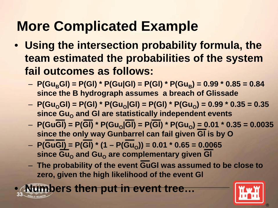
More Complicated Example • Using the intersection probability formula, the
team estimated the probabilities of the system fail outcomes as follows: – P(GuBGl) = P(Gl) * P(Gu|Gl) = P(Gl) * P(GuB) = 0.99 * 0.85 = 0.84
since the B hydrograph assumes a breach of Glissade – P(GuOGl) = P(Gl) * P(GuO|Gl) = P(Gl) * P(GuO) = 0.99 * 0.35 = 0.35
since GuO and Gl are statistically independent events – P(GuGl) = P(Gl) * P(GuO|Gl) = P(Gl) * P(GuO) = 0.01 * 0.35 = 0.0035
since the only way Gunbarrel can fail given Gl is by O – P(GuGl) = P(Gl) * (1 – P(GuO)) = 0.01 * 0.65 = 0.0065
since GuO and GuO are complementary given Gl – The probability of the event GuGl was assumed to be close to
zero, given the high likelihood of the event Gl
• Numbers then put in event tree…

34
More Complicated Example • Given the 1000-year flood, the five system
outcomes should be ME and CE: • The fact that their conditional probabilities sum
to 1.2 indicates that there is still intersection • Intersection a result of the way that the system
probabilities were estimated (but best we can do without a time-dependent fragility curve)
• Solution: apply CCA

35
More Complicated Example • Common Cause Adjustment
(CCA) resolves the intersection by adjusting the “sizes” of the individual events
• Total probability of the union (in this case 1.0) remains the same
• Not an exact solution, but better than double counting the intersection in risk estimates
• For a set of ME and CE outcomes, simply divide each probability by the apparent total (1.20)

36
More Complicated Example • Once the probabilities of the system outcomes
have been adjusted, the next step would be to estimate the life loss for each system outcome, calculate the annualized life loss, and “reallocate” risk back to the individual dams
• After doing that, the team would be ready to start developing corrective action alternatives for the system

37
Most complicated example • Given:
– 2 dam system, both embankments. - • Dam A (upstream). • Dam B (downstream).
Dam A (embankment)
Dam B (embankment)
Flood u/s of Dam A.Flood between Dam A and Dam B - Hydrograph could be Dam A releases + intervening flows; Dam A breach hydrograph w/ or w/o intervening flows. Flood d/s of Dam B -
Hydrograph could be Dam B releases; Dam B breach hydrograph as a result of Dam A failing or not failing.
Illustration - Existing Dam System

38
Most complicated example System Description
Dam A: Dam B: • Reservoir – 1,000,000 ac-ft. • Reservoir – 45,000 ac-ft.
• Zoned embankment – HSTR = 200 ft., LCREST = 1,400 ft.
• Zoned embankment – HSTR = 90 ft., LCREST = 2,500 ft.
• Spillway – Location – reservoir rim, controlled (gated), QDESIGN = 75,000 ft3/s.
• Spillway – Location – right abutment, uncontrolled (ogee), QDESIGN = 25,000 ft3/s.
• Outlet Works – Location – right abutment tunnel, QDESIGN = 7,500 ft3/s.
• Outlet Works – Location – left abutment tunnel, QDESIGN = 3,000 ft3/s.
• Powerplant – Location – Wyes off of OW near d/s portal, QDESIGN
= 3,000 ft3/s.

39
Most complicated example
• Individual Dams Approach - Hydrology and Flood Routing: – Both Dam A and B periodically evaluated as part
of the Dam Safety Program. – Seasonal frequency floods and PMFs have been
developed. • Rain-on-snow (Feb through mid-Jun). • Thunderstorm (mid-Jun through Aug).
– Basic flood routings available for both dams. • Frequency flood routings through Dam A over a range of
starting RWSs. • Operation flood (Dam A releases + intervening flows w/o
Dam A failing) routings through Dam B over a range of starting RWSs.

40
Most complicated example
• Individual Dams Approach - Consequences: – Incremental consequences for hydrologic PFMs –
difference between life loss due to breach outflows (dam failure) and max. operation outflows (non-dam failure).
– Available inundation data/maps may not fit exact situation being evaluated.
• Inundation studies for both max. operation releases and breach outflows for Dam A and B were available.
• Incremental consequences summary includes: – Dam A (includes Dam B breach) – Life loss = 100. – Dam B only – Life loss = 60.

41
Most complicated example
• Individual Dams Approach - Baseline RA: – Overtopping fragility curves developed for each dam. – Overtopping PFM event trees were developed for
each dam, which included initial RWS ranges, flood loading ranges, and conditional breach probabilities based on fragility curves.
• For Dam A: AFP = 7.35E-6, ALL = 7.35E-4. • For Dam B: AFP = 6.46E-5, ALL = 3.87E-3.
– Based on risk estimates • For Dam A, no further action taken. • For Dam B, SOD recommendation made, that led to IE and
CAS to reduce risks.
Unadjusted non-system (individual dam) estimates

42
Most complicated example • Individual Dams Approach - Risk Reduction
for Dam B: – Ability to pass at least a 500,000-yr rain-on-snow
flood would reduce risks to acceptable levels and so this flood was identified as the IDF.
– Both non-structural and structural alternatives were evaluated. The recommended alternative cost estimate was $45,000,000 and included
• 20-ft dam raise. • Replace existing uncontrolled spillway w/ controlled
(top-seal radial gate) spillway w/ larger discharge capacity.
• Relocate/modify existing infrastructure located along the reservoir rim.

43
Most complicated example
• Individual Dams Approach- Risk Reduction for Dam B (cont’d): – Incremental consequences for both Dam A and
Dam B remained unchanged from the consequences associated w/ the existing conditions.
– Overtopping fragility curves developed for Dam A were unchanged, but revised for Dam B mod.
– Overtopping PFM event trees were developed for each dam, which included initial RWS ranges, flood loading ranges, and conditional probabilities based on fragility curves.
• For Dam A: Same as existing conditions. • For Dam B: AFP = 1.88E-6, ALL = 1.13E-4.
Unadjusted non-system (individual dam) estimates

44
Most complicated example
• Individual Dams Approach - Risk Reduction for Dam B (cont’d): – Although risk reduction can be achieved via the
proposed alternative, costs were considered very significant (due primarily to relocating/modifying existing infrastructure).
– To determine if there was a more cost-effective alternative, the risk reduction efforts were broadened to a system evaluation.

45
Most complicated example
• Dam System - Hydrology: – Seasonal frequency floods
and PMFs were developed for both dams (rain-on-snow controls).
– Breach floods were developed as part of a fully dynamic hydraulic model (MIKE21).

46
Most complicated example
• Dam System - Flood Routings: – Flood routings through both dams.
• Frequency flood routings through Dam A over a range of starting RWSs were performed.
• Operation flood (Dam A releases + intervening flows w/o Dam A failing) and breach hydrograph routed d/s to Dam B, then through Dam B over a range of starting RWSs.
• Due to lag time estimates, multiple-peak hydrographs (time separation between operation flood and breach flood) were determined to be most likely.
0
10,000
20,000
30,000
40,000
50,000
60,000
70,000
80,000
90,000
012
2436
4860
7284
96108
120
Time (hours)
Discharge (ft3/s)
Dam
A B
reach Hydrograph (capable of failing
Dam
B, but due to lag tim
e between D
am A
breach hydrograph and D
am B
operations hydrograph, D
am B
may have already failed
by the time that D
am A
breach hydrograph reaches D
am B
).
Dam
B O
perations Hydrograph, w
hich is a com
bination of Dam
A operation
releases + intervening flows (capable of
failing Dam
B before or at the sam
e tim
e Dam
A fails).
Lag T
ime betw
een H
ydrograph Peaks

47
Most complicated example
• Dam System - Consequences: – Incremental consequences varied from the
individual dams evaluations for Dam A and Dam B.
– Changes resulted from outcome associated with Dam A failing and Dam B not failing and due to the multiple-peak hydrographs.
– Incremental consequences summary: • Dam A (includes Dam B breach) – Life loss = 100. • Dam A (without Dam B breach) – Life loss = 80. • Dam B (multiple-peak hydrograph) – Life loss = 60.

48
Most complicated example
• Dam Systems - Existing (baseline) RA: – Overtopping fragility curves developed for the
individual dams evaluation were used for the system evaluation.
– Overtopping PFM event tree was developed for dam system, which included initial RWS ranges, flood loading ranges, and conditional breach probabilities based on fragility curves.
• For Dam System: AFP = 6.87E-5, ALL = 4.15E-3. • For Dam A: AFP = 7.86E-7, ALL = 7.85E-5. • For Dam B: AFP = 6.82E-5, ALL = 4.09E-3.
– Outcome from risk estimates. • Based on Dam A and B risks for Dam System A-B, SOD
recommendation made, that led to IE and CAS to reduce system risks.
Adjusted system individual dam estimates

49
Most complicated example
• Dam Systems - Risk Reduction Dam A-B: – Three dam system structural modifications were
considered, including (reported risks are for the entire system).
• Modify Dam B only. – Same modification as noted for the individual dams evaluation. Summary includes: $45,000,000 cost, AFP = 7.36E-6, and ALL = 4.71E-4.
• Modify Dam A only. – 8-ft dam raise and increased releases through existing controlled (top-seal radial gate) spillway. Summary includes: $28,000,000 cost, AFP = 1.39E-5, and ALL = 8.38E-4.
• Modify Dam A only with Re-operation. – 10-ft dam raise and limit releases through existing controlled spillway. Summary includes: $30,000,000 cost, AFP = 2.00E-5, and ALL = 1.27E-4.
50
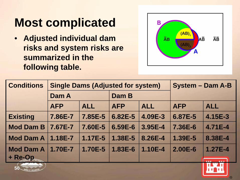
Most complicated • Adjusted individual dam
risks and system risks are summarized in the following table.
Conditions Single Dams (Adjusted for system) System – Dam A-B
Dam A Dam B AFP ALL AFP ALL AFP ALL
Existing 7.86E-7 7.85E-5 6.82E-5 4.09E-3 6.87E-5 4.15E-3 Mod Dam B 7.67E-7 7.60E-5 6.59E-6 3.95E-4 7.36E-6 4.71E-4 Mod Dam A 1.18E-7 1.17E-5 1.38E-5 8.26E-4 1.39E-5 8.38E-4 Mod Dam A + Re-Op
1.70E-7 1.70E-5 1.83E-6 1.10E-4 2.00E-6 1.27E-4

51
Most complicated example
• Dam Systems - Risk Reduction – Adjusted individual
dam and dam system risks (pre- and post-mod) as depicted in the Reclamation f-N Chart.
Existing Conditions
Modified Dam B
Modified Dam A
Modified Dam A+

52
Most complicated example
• Conclusions: • Modify Dam B only option – very expensive system fix,
and so was not pursued. • Modify Dam A only option – least cost system fix, but
transfers some risk downstream to Dam B due to increased Dam A discharges. This alternative was not pursed.
• Modify Dam A only with re-operation – although a bit more expensive than the “modify Dam A only” alternative, considerably more risk reduction results. It was decided that the added system risk reduction was well worth the additional cost.

53
The End