Best Practices for Pressure Transient Tests Using Surface Based Measurements

Dieter Becker and Jim McCoy, Echometer Company

A. L. Podio, University of Texas

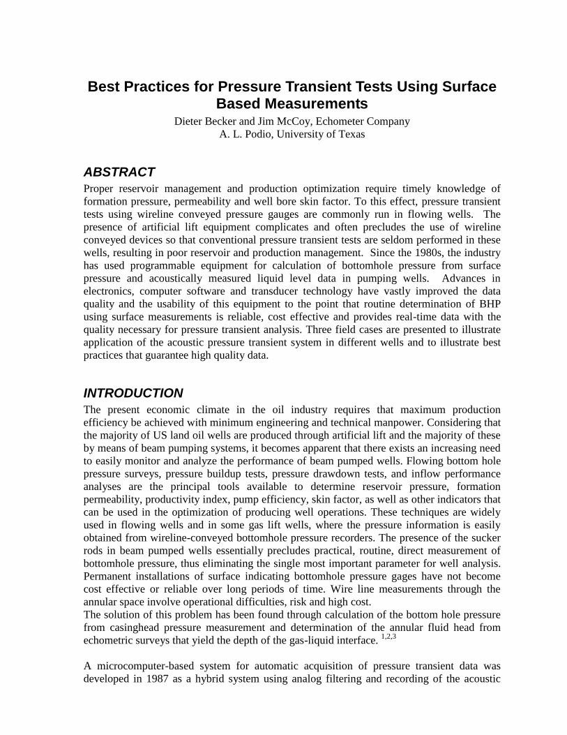
ABSTRACT

Proper reservoir management and production optimization require timely knowledge of

formation pressure, permeability and well bore skin factor. To this effect, pressure transient

tests using wireline conveyed pressure gauges are commonly run in flowing wells. The

presence of artificial lift equipment complicates and often precludes the use of wireline

conveyed devices so that conventional pressure transient tests are seldom performed in these

wells, resulting in poor reservoir and production management. Since the 1980s, the industry

has used programmable equipment for calculation of bottomhole pressure from surface

pressure and acoustically measured liquid level data in pumping wells. Advances in

electronics, computer software and transducer technology have vastly improved the data

quality and the usability of this equipment to the point that routine determination of BHP

using surface measurements is reliable, cost effective and provides real-time data with the

quality necessary for pressure transient analysis. Three field cases are presented to illustrate

application of the acoustic pressure transient system in different wells and to illustrate best

practices that guarantee high quality data.

INTRODUCTION

The present economic climate in the oil industry requires that maximum production

efficiency be achieved with minimum engineering and technical manpower. Considering that

the majority of US land oil wells are produced through artificial lift and the majority of these

by means of beam pumping systems, it becomes apparent that there exists an increasing need

to easily monitor and analyze the performance of beam pumped wells. Flowing bottom hole

pressure surveys, pressure buildup tests, pressure drawdown tests, and inflow performance

analyses are the principal tools available to determine reservoir pressure, formation

permeability, productivity index, pump efficiency, skin factor, as well as other indicators that

can be used in the optimization of producing well operations. These techniques are widely

used in flowing wells and in some gas lift wells, where the pressure information is easily

obtained from wireline-conveyed bottomhole pressure recorders. The presence of the sucker

rods in beam pumped wells essentially precludes practical, routine, direct measurement of

bottomhole pressure, thus eliminating the single most important parameter for well analysis.

Permanent installations of surface indicating bottomhole pressure gages have not become

cost effective or reliable over long periods of time. Wire line measurements through the

annular space involve operational difficulties, risk and high cost.

The solution of this problem has been found through calculation of the bottom hole pressure

from casinghead pressure measurement and determination of the annular fluid head from

echometric surveys that yield the depth of the gas-liquid interface. 1,2,3

A microcomputer-based system for automatic acquisition of pressure transient data was

developed in 1987 as a hybrid system using analog filtering and recording of the acoustic

signal4, 5

. Such system still depended in some measure on the operator’s interpretation of the

acoustic chart recordings to determine the average acoustic velocity in the annular gas.

The present system is a fully digital data acquisition and processing package which

automatically determines the position in time of the gas-liquid interface, digitally filters the

acoustic data to enhance collar reflections and calculates the depth to the liquid level from

the acoustic velocity obtained from a count of collar reflections. Operation is pre

programmed by the user.

DESCRIPTION OF THE DIGITAL ACOUSTIC PRESSURE TRANSIENT SYSTEM

The Automatic Acoustic Pressure Transient system is based on the Digital Well Analyzer1

configured for long term unattended operation and controlled by software specially

developed for pressure transient data recording and analysis. Figure (1) depicts a schematic

diagram illustrating the various components of the system. The equipment consists of an

electronic package that includes a computer, analog to digital converter, amplifying and

conditioning circuits. This is connected to the wellhead assembly with interconnecting

cables. A 12-volt battery and a large gas supply container are the needed power sources.

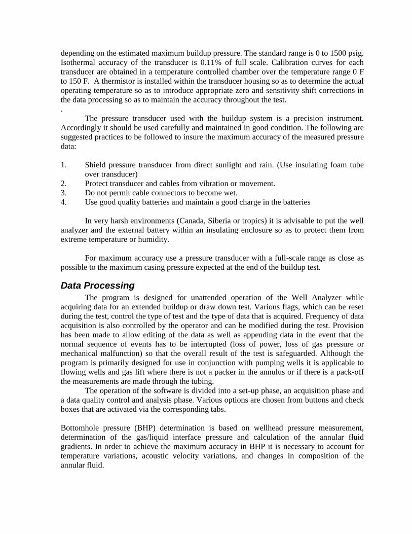
Figure (2) illustrates the functional relationships between these elements. Note that the data

acquisition and processing package can be also used in conjunction with dynamometer and

other sensors if desired.

The Acoustic Source / Detector

This wellhead assembly consists of a microphone, solenoid gas valve, pressure transducer

and volume chamber. Nitrogen gas is readily available and commonly used.

Signal Acquisition, Processing and Recording

A good 100 amp-hour, 12 volt, deep-cycle battery should be used. A battery that is

fully charged will last two or three days at normal temperatures. The Well Analyzer will

drain the battery approximately 0.007 volts per hour or 0.17 volts/day. The initial A/D

battery voltage when beginning pressure transient testing is approximately 11.6 volts. This

battery voltage is indicated on the main analysis screen that is displayed during the test. A

record of A/D battery voltage vs. time is available in the plotting routines. The battery

voltage vs. time display screen can be used to estimate the remaining battery life. The voltage

drops linearly to 10.2 volts and then drops rapidly. The estimated remaining battery life is

calculated by utilizing the battery drain rate, the last voltage reading and then predicting

when the voltage will drop to 10.2 volts. Data acquisition ceases when the voltage drops to

10.0 volts. Please use this analysis procedure to verify that the computer, A/D battery and

external 12 volt deep-cycle battery are all operating normally and in good condition. The

amplifier, A/D converter are not allowed to acquire data when the battery voltage is less than

10 volts.

Transducers

A high accuracy strain gage pressure transducer provides a signal proportional to pressure.

Direct connection to the wellhead assembly is through a quick-connector so that casinghead

pressure can be monitored continuously during the test. Various pressure ranges can be used

depending on the estimated maximum buildup pressure. The standard range is 0 to 1500 psig.

Isothermal accuracy of the transducer is 0.11% of full scale. Calibration curves for each

transducer are obtained in a temperature controlled chamber over the temperature range 0 F

to 150 F. A thermistor is installed within the transducer housing so as to determine the actual

operating temperature so as to introduce appropriate zero and sensitivity shift corrections in

the data processing so as to maintain the accuracy throughout the test.

.

The pressure transducer used with the buildup system is a precision instrument.

Accordingly it should be used carefully and maintained in good condition. The following are

suggested practices to be followed to insure the maximum accuracy of the measured pressure

data:

1. Shield pressure transducer from direct sunlight and rain. (Use insulating foam tube

over transducer)

2. Protect transducer and cables from vibration or movement.

3. Do not permit cable connectors to become wet.

4. Use good quality batteries and maintain a good charge in the batteries

In very harsh environments (Canada, Siberia or tropics) it is advisable to put the well

analyzer and the external battery within an insulating enclosure so as to protect them from

extreme temperature or humidity.

For maximum accuracy use a pressure transducer with a full-scale range as close as

possible to the maximum casing pressure expected at the end of the buildup test.

Data Processing

The program is designed for unattended operation of the Well Analyzer while

acquiring data for an extended buildup or draw down test. Various flags, which can be reset

during the test, control the type of test and the type of data that is acquired. Frequency of data

acquisition is also controlled by the operator and can be modified during the test. Provision

has been made to allow editing of the data as well as appending data in the event that the

normal sequence of events has to be interrupted (loss of power, loss of gas pressure or

mechanical malfunction) so that the overall result of the test is safeguarded. Although the

program is primarily designed for use in conjunction with pumping wells it is applicable to

flowing wells and gas lift where there is not a packer in the annulus or if there is a pack-off

the measurements are made through the tubing.

The operation of the software is divided into a set-up phase, an acquisition phase and

a data quality control and analysis phase. Various options are chosen from buttons and check

boxes that are activated via the corresponding tabs.

Bottomhole pressure (BHP) determination is based on wellhead pressure measurement,

determination of the gas/liquid interface pressure and calculation of the annular fluid

gradients. In order to achieve the maximum accuracy in BHP it is necessary to account for

temperature variations, acoustic velocity variations, and changes in composition of the

annular fluid.

Temperature Correction

During the several days of the typical well test, the transducer’s sensing element may

undergo temperature variations of over 60 degrees F. Even though the transducer is built with

integral temperature compensation this temperature change can cause considerable (+/- 2%)

variations in the measurement of casing head pressure that are reflected in the BHP record.

Additional correction is applied, by measuring the transducer temperature with a thermistor

and computing the corresponding pressure deviation from calibration curves obtained for

each individual transducer, to eliminate most of the interfering pressure oscillations.

Acoustic Velocity Variation

During the well test (buildup or drawdown) the pressure, temperature and component

distribution of the gas in the annulus will undergo significant changes. These in turn will

cause variations in the acoustic velocity of the gas. At any given time the average acoustic

velocity is obtained from an automatic count of filtered collar reflections, when available,

and the average joint length. For wells where the acoustic record does not show collar

reflections, the variation of acoustic velocity is computed from the known gas gravity the

average temperature and the measured pressure.

Experience indicates that pressure-dependent velocity variations occur gradually and

continuously, as shown in Figure (3). The data reduction program interpolates between these

points to calculate the depth to the gas/liquid interface from the measurement of the travel

time of the liquid echo. If this variation were not taken into account and a single value for

acoustic velocity were used in interpreting the travel time data a significant error in

calculated BHP would be made.

Annular Fluid Composition

Several papers have been presented on the correct methods for calculation of bottomhole

pressure from acoustic determination of annular liquid levels. The BHP is the sum of the

casing head pressure and the hydrostatic column pressures due to the annular gas and liquid.

The gas column gradient is calculated as a function of pressure, temperature and gas gravity.

The liquid column pressure is a function of the composition of the liquids, and the in-situ

water/oil ratio and gas/liquid ratio. Flowing conditions and well geometry determine the fluid

distributions. For example for steady state pumping conditions the liquid above the pump

intake is oil due to gravity segregation occurring in the annulus. When the well is shut in for

a buildup the water cut remains essentially constant during the after flow period and a

moving oil/water interface develops during the test. These factors are taken into

consideration by the program in calculation of the bottomhole pressure. In-situ oil and water

densities are calculated as a function of pressure and temperature using conventional

correlations.6

When the producing bottomhole pressure is below the bubble point, free gas is produced

from the reservoir and is generally vented from the annulus. This annular gas production

reduces the liquid column gradient and thus has to be taken in consideration in the BHP

calculation. Experience indicates that a gaseous liquid column can extend for a significant

period of time after the well is shut in. A correlation derived from a multitude of field

measurements of gaseous liquid column gradients3 is used to account for this effect. When a

long annular gaseous liquid column is present in a pumping well, to obtain the most accurate

results, it is recommended that before the initiation of the buildup test the liquid level be

depressed to a few joints above the pump by increasing the casing head back pressure while

maintaining a steady pumping rate. This is easily achieved by means of an adjustable

backpressure regulator installed on the casing head valve that will maintain the casing

pressure constant during the process of liquid level depression until stabilization. The result

will be that at the end of the after flow period the height of the liquid column will be

minimized and a major portion of the BHP will be provided by the surface casing pressure

(that is measured very accurately) and the gas column pressure.

Best Practices

Running a pressure buildup test involves a major commitment of time and manpower as well

as temporary loss of income while the well is shut-in. Therefore every effort should be made

to guarantee that the final data is of sufficient good quality to yield an accurate representation

of the formation permeability, skin and static reservoir pressure. The following

recommended procedures provide guidelines to help reach that objective. Although the

procedure makes reference to the Well Analyzer, it is understood that it is applicable to tests

undertaken with other acoustic fluid level instruments.

Beam Pumped Wells

1- Obtain all necessary data for acquisition and pressure transient analysis. Review and

update base well file. Obtain or draw a well bore diagram to identify all changes in annular

cross section that could be used as down hole markers or that could interfere with automatic

liquid level selection (liners, tubing cross-overs, etc.)

2- Prior to date of well test, perform acoustic measurements to determine normal

producing conditions, acoustic velocity, casing pressure and existence of a gaseous liquid

column. Perform dynamometer test to determine pump fillage and effective pump

displacement.

3- If height of gaseous liquid column is significant perform a short duration (1hour)

liquid level depression test (by closing the casing to flow line valve) to estimate the time

required to depress the liquid level to the pump intake.

4- Inspect all well connections to flow lines, casing head, tubing head, stuffing box,

condition of valves, leaks etc. and report any problems to the operator so that they may be

fixed before date of well test. It is important that the SV is holding otherwise there will be

excessive back flow of liquid from the tubing, during the early stages of the buildup and this

will show up as additional after-flow.

5- Shortly before (24-48 hours) date of test put the well on a production test in order to

determine the average 24-hour production rate, water cut and GOR.

6- Review and update all data and prepare test procedure and check list.

7- If gaseous liquid column depression is to be performed, install back pressure

regulator on casing to flow line outlet (if possible) and start increasing casing head pressure

while monitoring liquid level. Use the pressure transient module to monitor depression test).

This may take several hours or days as estimated in step 3. This should continue until the

fluid level is indicated to be about 60 feet above the pump intake. When this is reached the

casing pressure should be stabilized to a constant value (+/- 5% of the measured value)

8- Make sure all batteries are charged before starting the test. On the day of the test after

setting up the equipment take a fluid level to verify that all is normal. Take a dynamometer

and verify that the pump fillage and operation is the same as was established in step 2 and

agrees with the well test information. If the difference is more than 10% continue monitoring

the dynamometer during 30 minutes to detect any abnormalities. If the pump operation is

erratic, then postpone the test until the problem is fixed since it would be impossible to

determine an accurate well flow rate that is needed for pressure buildup interpretation.

9- Verify that all connections between the gas bottle and the remote fire gun do not have

any leaks. Check all electrical connectors for tightness and protect them from rain. Place a

thermal insulating tube on the pressure transducer. Check connection to external battery and

verify that the Well Analyzer (EXT BAT) light is on and the charger cable is connected to

the laptop.

10- Start the TWM program and go through the Set Up procedure to get the zero offset of

the pressure transducer. Select the Transient Test module and complete the test set up

procedure. Use Logarithmic schedule unless there is a reason for selecting otherwise. Take a

Pre-Shot and verify that the program is picking the fluid level correctly (adjust the signal

window if necessary) and that the acoustic velocity and fluid level depth are computed

correctly as established earlier (steps 7 and 8)

11- Start the buildup acquisition (START acoustic transient test) while the well is still

pumping (first pressure value corresponds to PBHP). As soon as the program completes the

processing of the first shot STOP the pump. Set brake and lock out the motor switch. Close

tubing flow valve to prevent the well to flow as the pressure builds up during the test.

12- Monitor the progress of the test at least for 30 minutes and check that the fluid level

is picked correctly and all the data is consistent (fluid level may rise or fall depending on

well conditions) especially the casing pressure should show a consistent trend. Make any

adjustments to obtain accurate time to liquid level as described in the TWM manual.

13- Determine the rate of casing pressure increase (psi/hour) to estimate the likely casing

pressure for the time when you will return to the well to check the test progress. Set the

regulator pressure to 200 psi above the estimated future casing pressure to insure that fluid

level shots will be taken at that time.

14- Check that the EXT. POWER indicator is lit, check all connections before leaving the

well. Check that the laptop power management has been set to NEVER turn off the laptop

and that the laptop will stay ON even when closing the lid. Close well analyzer case and

protect from the environment. Wait until a shot is taken automatically before leaving the

site.

15- When returning to the well, open the Well Analyzer and the laptop. Check the

Progress screen and verify when the last shot was taken, when the next shot is due, the

presence of soft shots (S), the casing pressure, time to liquid, etc. Take a MANUAL shot and

observe the liquid level pick and depth calculation. Check a time plot of Casing Pressure vs.

time and observe if there are any anomalies (step changes of pressure or abrupt changes of

slope) that may indicate the presence of leaks at the wellhead or transducer problems.

16- Make necessary adjustments to obtain accurate fluid level and depth values in

subsequent shots.

17- Determine casing pressure increase rate and adjust regulator pressure. Check the

pressure in Nitrogen bottle and battery voltage and replace them as necessary.

18- Copy all the data recorded to this point to a diskette, CD or USB removable memory

as appropriate to the laptop in use. The objective is to transfer the data to an office computer

for further analysis to determine if the test has run sufficiently for meaningful buildup

interpretation or if the test should be continued.

19- If the test continues go back to step 14.

20- If the test is terminated, take a MANUAL shot and when the computer finishes

processing the data select END Transient Test and exit the Pressure Transient Module.

21- Select the Acoustic Test module, select ―shut-in‖ to indicate the well status ad take an

acoustic record to establish the present value of Static Bottom Hole Pressure in the well base

file.

22- Select Dynamometer Test. Connect the PRT to the polished rod. Open the tubing

valve to the flowline, release the brake and start pumping unit.

23- Make dynamometer measurements to determine that the pump is operating normally.

24- Open slowly the casing valve to the flowline to SLOWLY reduce the casing pressure

to its normal operating value. See NOTE below for ESP wells.

25- After the casing pressure has stabilized, repeat dynamometer measurements to verify

that the pump is operating normally. If not then notify the operator of the problems that may

be indicated.

26- If all is normal, stop the pumping unit, disconnect dynamometer and remote fire gun.

Transfer all data to external storage.

27- Start unit and verify that all is normal before leaving well site.

ESP and PCP Wells

For wells produced with ESPs or PCPs the steps related to dynamometer measurements are

not relevant. For ESP wells it is very important to reduce the casing pressure very slowly

since gas will dissolve in the down-hole cable’s insulation as the pressure in the annulus

increases during the buildup test. A rapid reduction of casing pressure will cause the

insulation to swell and possibly damage the cable. A slow decrease in casing pressure allows

the dissolved gas to evolve gradually without causing swelling of the insulation.

Gas-Lift Wells

Fluid level measurements are made through the tubing. Annular fluid level is monitored

before shut-in and then periodically to observe any changes in pressure or fluid level during

the transient test. After completing the fluid level test the remote fired gas gun is installed on

the tubing, preferably above the swab valve (when present) after removing any needle valve

and replacing it with a fully opening ball valve. Injection of the gas into the casing is stopped

and the valve from the tubing to the flow line is closed. Acoustic single shots are taken

manually at 3 to 5 minutes intervals until a clear fluid level echo is observed. Then the

pressure transient module is used to set up automatic acquisition of the data from that point

onwards.

Gas Wells

Wells that are producing gas through tubing with no packer in the annulus

Pressure transient measurements should be done in the annulus since there will be a

minimum of liquid accumulated above the tubing intake. Fluid level measurements should be

taken before stopping the flow from the tubing to establish the position of the liquid level in

the annulus and to observe any variations during normal flowing conditions.

Wells that are producing gas through tubing with a packed-off annulus

Procedure is similar to that described above for Gas-Lift wells.

Wells that are producing gas through the annulus and dewatered through tubing

Procedure is similar to that recommended for pumping wells

Wells that are producing gas through both tubing and annulus

Preferred method is to undertake the pressure transient measurements through the annulus.

These wells will exhibit a longer after flow and well bore storage effect that those wells

producing through tubing and have a packed-off annulus.

Presentation of Results

At any time during and/or after the test it is possible to obtain graphical and tabular

presentation of the data and the calculated results.

The type of presentation is selected from options in the data presentation menu. These

include:

Casing head pressure vs. time

Bottomhole pressure vs. time

Liquid level vs. time

Transducer temperature vs. time

Acoustic round trip time (seconds) vs. time

Acoustic Frequency (Jts/sec) vs. time

MDH—BHP vs. Log(time)

Horner

Log-Log analysis

Liquid after flow vs. time

Gas after flow vs. time

Smoothed velocity vs time

Battery voltage vs time

In all the transient plots, utilities are made available to aid in the interpretation. These include

least square line fits of selectable portions of the data, unit slope and half slope trend lines,

zooming to portions of the data and calculation of time derivatives.

The purpose of the pressure transient interpretation graphs is to provide a real time analysis

to determine whether the test has been carried long enough to the point when interpretation

of the data will yield accurate values of skin, permeability and reservoir pressure.

RESULTS OF FIELD TESTS

The Automatic Acoustic Bottomhole Pressure System has been used for many years and for a

variety of situations and environmental conditions. Following are presented a selection of

field data with the purpose to illustrate the variety and quality of the data that has been

obtained.

Well A

Figures 4 (a-e) illustrate the data obtained during a seven-day pressure buildup test in a 4900-

ft beam pumping well. Production prior to shut-in was 226 water, 36 oil in Bbl/D and 24

MSCF of gas. A total of 197 fluid level measurements were recorded. Data was appended

one time. Figure 4a shows the measured casing head pressure increasing throughout the test

caused by continued influx of gas. The pressure transducer temperature exhibits daily

variations as large as 40 degrees F but temperature compensation and calibration eliminates

any effect on the pressure data. Figure 4b shows the rise in liquid level of about 3000 feet

experienced during the liquid after flow period that seems to end at about 5000 minutes

where the liquid level stabilizes at about 1900 feet. Figure 4c shows the computed BHP that

is used to generate the Log-Log plot shown in Figure 4d where the unit slope line and the

derivative indicate that the well bore storage effect ends at about 20 hours. The

corresponding Horner plot shown in Figure 4e shows a small skin of 0.8 and a P* = 2018 psi.

Well B

Figures 5 (a-d) illustrate results of a 4-1/2 day buildup test in a PC pumped oil well

producing 80 Bbl/D oil from a depth of 3150 feet. Data was appended 6 times due to poor

external battery quality and a total of 136 fluid level shots were taken. Figure 5a shows that

liquid level increased by about 2600 feet and casing head pressure built by 380 psi during the

test. The x points in the figure correspond to bad data due to occasional misfiring of the

remote fire gas gun for lack of sufficient gas supply pressure or other problems. They are not

included in the calculations but are a part of the permanent record and are shown for data

quality control. The computed BHP and liquid after flow are plotted in Figure 5b that shows

the leveling off of the after flow at about 48 hours and the corresponding near-stabilization of

the BHP. The Log-Log plot in Figure 5c shows by the end of the test the radial flow period is

just beginning and that probably the test was ended prematurely. The Horner plot in Figure

5d is characteristic of a severely damaged well with a skin near 9 and a P*=1306 psi.

Well C

Figures 6a through 6c show the results of a buildup test extending 25 days and 17 hours. A

total of 831 shots were taken and the data set was appended 61 times. The pumping well is

completed with 7 inch casing and 2-7/8 inch tubing and was producing 16 Bbls/day oil from

a 12 ft pay zone at a formation depth of 5379 feet. Figure 6b shows a very smooth decrease

of the round trip travel time as the depth to the liquid level rises from 4998 feet at shut-in to

1916 feet at the end of the test. The bottom hole pressure increases from 168 to 1607 psi

during the same time period. Figure 6c shows the Log-Log plot of the BHP data and

indicates that the test was terminated prematurely since the derivative is changing and the

radial flow period has not been reached in spite of the lengthy test.

Well D

Figures 7a through 7c show the results of a buildup lasting 3 days and 13 hours in a well

producing 4 bbl of oil and 4 Mcf of gas per day from a 56 ft thick formation. A total of 235

shots were taken and the data was appended 4 times.

Well bore storage effects are overcome and the radial flow period is reached after about 8

hours of shut-in but then there is an increase of the derivative as seen in Figure 7b, that

indicates the presence of a boundary effect. Figure 7c shows that using the radial flow section

of the data the skin is estimated at S= 2 and P* yields 102 psia.

Well E

In this well 13 MSCF/D of gas are being produced by flow through the casing annulus while

24 Bbl/day of water is pumped via the tubing. Figure 8a shows that the gas flow appears to

continue throughout the test since the casing pressure continues to increase from 53 at the

start to 252 psia at the end while the liquid level rises only 25 feet. The net result is that the

computed BHP essentially mirrors the increase in casing pressure as seen in figure 8b. The

noise from the gas flow and the fact that the liquid level stayed below the upper required

manual analysis of several shots and the rejection of several points as indicated by the x’s in

Figure 8a. The resulting bottom hole pressure vs. time is shown in Figure 8b and the Log-

Log plot in Figure 8c shows that the test was carried out past the end of the well bore storage

effects and into the radial flow region.

Figure 8d shows the corresponding Horner plot that yields a skin = -0.5 and a P* = 330 psia.

This data set required some manual interpretation of the liquid level data due to the noise and

interference from echoes generated by the perforations since the liquid level was primarily

below the top perforations. Figure 8e is a plot of the RTTT to the liquid level as a function of

time. It shows that several data points do not follow the decreasing trend corresponding to the

rise in liquid level. The software allows manual interpretation of the acoustic record that is

reproduced in Figure 8f and that corresponds to the data point flagged by the dashed vertical

marker in Figure 8e. The record shows that the liquid level is not properly selected

automatically by the software due to the presence of a signal (caused by the perforations) that

precedes the arrival of the echo from the liquid level. Figure 8g shows how the liquid level

marker is adjusted to the correct first break of the liquid level echo. After the correction is

made, the data point in question now follows the expected RTTT trend as shown in Figure

8h. Similar corrections were carried out for the other outlying points prior to recomputing the

final values of BHP.

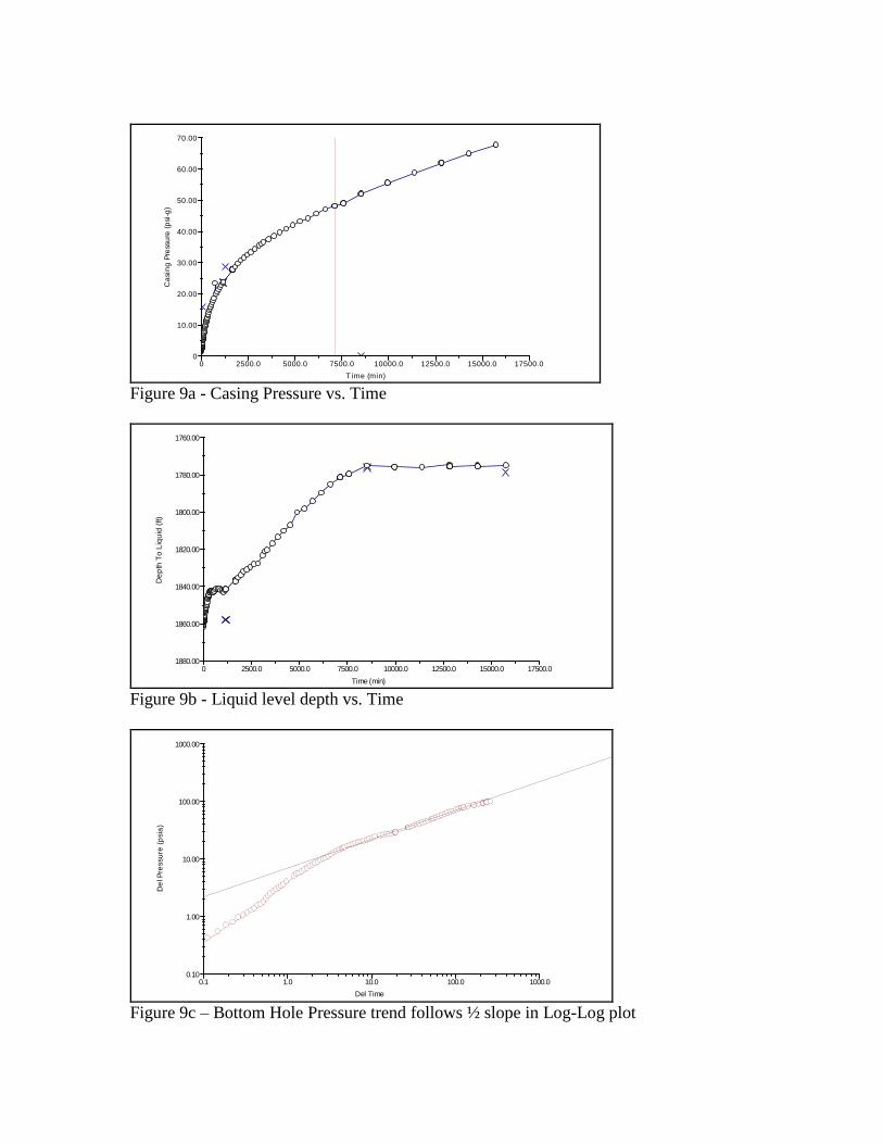
Well F

This well is a low production well (4 bbl/day oil) from a shallow formation (1800 feet) with

perforations over a 66 ft interval. The buildup test was carried out over 10 days and 22 hours.

A total of 116 shots were taken and the data was appended 17 times since the Well Analyzer

had to be used for dynamometer and fluid level measurements in other wells. Figure 9a

shows a very smooth increase of casing pressure from 1.5 psig to over 65 psig during the

buildup. The increase corresponds to continued gas after flow. Figure 9b shows a rapid

increase in fluid level at the beginning of the test followed by a constant rate of liquid inflow

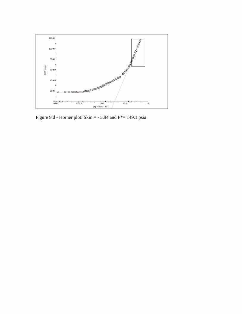
that stops after about 5 days into the buildup. The resulting Log-Log plot shown in Figure 9c

indicates a unit slope trend corresponding to a fractured reservoir. This is confirmed by the

Horner plot shown in Figure 9d that gives a negative skin near –6 and a P* = 149.1 psia.

Well G

This well is being produced with an ESP pump at a rate of 2211 Bbl/day water and 9 Bbl/day

oil from a depth pf 2900 feet completed with 5-1/2 inch casing and 2-7/8 tubing. The

producing interval covers 400 feet. A total of 90 shots were taken and the data was appended

once during the 26-hour buildup test. Figure 10a shows the variation of casing pressure

(circles) and liquid level (triangles) that show a relatively rapid increase in liquid level from

2800 to 800 feet in depth. The Log-Log plot in Figure 10b shows a decreasing derivative that

follows a brief radial flow period indicating the there is a constant pressure boundary. The

result of the Horner plot shown in Figure 10c indicates significant well bore damage with a

skin S= 8.44 and a P* = 1040 psia.

Well H

The buildup in this well is an example where the liquid level dropped to a deeper depth while

the casing pressure increased during the test. The well was producing 1 Bbl/day oil, 18

Bbl/day water and 50 MCF/D gas from a depth of 5020 feet. A rod pump is set at the bottom

of the producing interval at 5770 feet and initially the top of the gaseous liquid column is

observed at 4800 feet corresponding to the relatively high flow of gas from the annulus. The

collapse of the fluid column as the casing pressure increases is shown in Figure 11a. The

corresponding BHP computed at 5020 feet is seen to mirror the increase of casing pressure in

Figure 11b. The Log-Log plot in Figure 11c shows that the radial flow period may be just

beginning. As such the test should have been continued. The Horner plot shown in Figure

11d indicates that there may be significant skin but it is not possible to quantify with the

available data.

Well I

Figure 12 a shows the variation in casing pressure and liquid level in a water well producing

at a rate of 550 Bbl/day from a 10 ft formation at a depth of 1456 feet. Note the very rapid

700 ft increase of liquid level during the first hour accompanied by an increase in casing

pressure from 0.1 to about 20 psi. The corresponding BHP mirrors the increase of liquid level

as seen in Figure 12b. The resulting Log-Log plot shows that well bore storage effects are

overcome after 2-1/2 hours of shut-in. The dip in the derivative indicates the possibility of a

dual porosity formation. The Horner plot in figure 12d indicates a very large skin S=41 and a

P* = 434 psia.

SUMMARY

A digital pressure buildup data acquisition and processing system has been developed which

uses an acoustic liquid level instrument to determine the annular or tubular fluid distribution

while measuring the wellhead pressure. Unattended operation is made possible by the laptop

computer that controls the progress of the test according to a predefined schedule, records

and interprets the data and presents the information to the operator, in real time during the

test. The advanced electronics and pressure sensors used in the hardware result in a very

stable data acquisition system that operates reliably over extended periods of time. The

software that controls the acquisition and monitors the test progress offers the option of

interrupting data acquisition when the system is required for testing at other wells and

provides a reliable means of appending new data to the saved test while maintaining the time

relation to the beginning of the test.

The system has the overwhelming advantage over wireline-conveyed measurements that it

does not require entering the well bore but is totally based on surface measurements. Real-

time information regarding the progress of the pressure transient allows the operator to

decide on the best course of action to insure that the test will yield accurate and complete

data. Preliminary analysis of the data done at the well site can be followed up with detailed

transient analysis by exporting the BHP data vs. time to other analysis software.

REFERENCES

1. McCoy J. N., Podio A. L. and Dieter Becker: ―Pressure Transient Digital Data

Acquisition and Analysis From Acoustic Echometric Surveys in Pumping Wells‖

SPE 23980, Permian Basin Oil and Gas Recovery Conference, Midland, Texas,

March 18-20. 1992.

2. Mc Coy, J. N., Podio, A. L., Huddleston, K. L. and B. Drake:‖ Acoustic Static

Bottomhole Pressures,‖ SPE 13810, Production Operations Symposium, Oklahoma

City, OK, March 10-12, 1985.

3. Mc Coy, J. N., Podio, A. L., and K. L. Huddleston:‖Acoustic Producing Bottomhole

Pressures, SPE 14254, Annual Technical Conference and Exhibition, Las Vegas NV,

September 22-25, 1985.

4. Podio, A. L., McCoy, J. N. and Huddleston, K.L.: ‖Automatic Pressure Buildup Data

Acquisition and Interpretation Using a Microcomputer-based Acoustic Liquid Level

Instrument‖, SPE 16228 Presented at the SPE Production Operations Symposium,

Oklahoma City, OK, March8-10, 1987.

5. Podio, A. L. and J. N. McCoy: ―Computerized Well Analysis,‖ SPE 21174 presented

at the SPE Latin American Petroleum Engineering Conference, Rio de Janeiro,

October 14-19, 1990.

6. Hasan, A. R. and C. S. Kabir:‖ Determining Bottomhole Pressures in Pumping

Wells,‖ SPE 11580, Production Operations Symposium, Oklahoma City, OK,

February 27-March 1, 1983.

Figures

Figure 1 – Acoustic liquid level set-up for programmed automatic operation

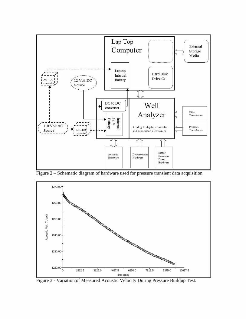
Figure 2 – Schematic diagram of hardware used for pressure transient data acquisition.

0 1562.5 3125.0 4687.5 6250.0 7812.5 9375.0 10937.51220.00

1230.00

1240.00

1250.00

1260.00

1270.00

Time (min)

Acoustic V

el. (

ft/s

ec)

Figure 3 - Variation of Measured Acoustic Velocity During Pressure Buildup Test.

0 1562.5 3125.0 4687.5 6250.0 7812.5 9375.0 10937.50

50.00

100.00

150.00

200.00

250.00

300.00

350.00

Time (min)

Casin

g P

ressure

(psi-g)

40.00

50.00

60.00

70.00

80.00

90.00

Pre

s. T

ransducer T

em

p. (D

eg F

)

Figure 4a – Long Term Pressure Buildup Test Showing Casing Pressure (circles) and

Transducer Temperature (triangles) as a function of elapsed time.

0 1562.5 3125.0 4687.5 6250.0 7812.5 9375.0 10937.50

50.00

100.00

150.00

200.00

250.00

300.00

350.00

T ime (min)

Ca

sin

g P

ress

ure

(p

si-g

)

1000.00

2000.00

3000.00

4000.00

5000.00

6000.00

De

pth

To

Liq

uid

(ft)

Figure 4b – Depth to Liquid level (triangles) and Casing head pressure (circles) vs. Time

0 1562.5 3125.0 4687.5 6250.0 7812.5 9375.0 10937.50

50.00

100.00

150.00

200.00

250.00

300.00

350.00

Time (min)

Casin

g P

ressure

(psi-g)

0

312.50

625.00

937.50

1250.00

1562.50

1875.00

BH

P (p

si-a

)

Figure 4c –Computed BHP (triangles) and Measured Casing head Pressure (circles) vs time

0.1 1.0 10.0 100.0 1000.010.00

100.00

1000.00

10000.00

Del Time

Del P

ressure

(psia

)

Figure 4d -Resulting Log-Log plot of Delta Pressure with Derivative vs. Delta time in hours

1.010.0100.01000.010000.00

250.00

500.00

750.00

1000.00

1250.00

1500.00

1750.00

(T p + del t) / del t

BH

P (

psi

a)

Figure 4e – Horner plot yields Skin= 0.8 and P*= 2018 psi

0 1250.0 2500.0 3750.0 5000.0 6250.0-100.00

0

100.00

200.00

300.00

400.00

500.00

Time (min)

Ca

sin

g P

ressu

re (

psi-

g)

1000.00

1500.00

2000.00

2500.00

3000.00

3500.00

4000.00

De

pth

To

Liq

uid

(ft)

Figure 5a - Liquid level (triangles) increases 2600 feet and Casing pressure (circles) builds

up 378 psi during 4-1/2 days test.

0 1250.0 2500.0 3750.0 5000.0 6250.00

250.00

500.00

750.00

1000.00

1250.00

1500.00

Time (min)

BH

P (

psi-

a)

-62.50

0

62.50

125.00

187.50

250.00

312.50

Liq

uid

Afte

rflow

(BB

L/D

)

Figure 5b -BHP(circles)levels off and Liquid after flow (triangles) tends to zero after about

48 hours

1.0 10.0 100.0 1000.01.00

10.00

100.00

1000.00

10000.00

Del Time

Del P

ressure

(psia

)

Figure 5c - Resulting Log-Log plot of Delta Pressure with Derivative vs. Delta time in hours

1.010.0100.01000.010000.00

250.00

500.00

750.00

1000.00

1250.00

1500.00

(Tp + del t) / del t

BH

P (

psia

)

Figure 5d - Horner plot shows skin of 8.9 and P*=1306 psi

0 6250.0 12500.0 18750.0 25000.0 31250.0 37500.00

62.50

125.00

187.50

250.00

312.50

375.00

437.50

Time (min)

Ca

sin

g P

ressu

re (

psi-

g)

60.00

70.00

80.00

90.00

100.00

110.00

Pre

s. T

ran

sd

uce

r Te

mp

. (De

g F

)

Figure 6 a –Variation of casing pressure and transducer temperature (triangles) during a 25

days and 17 hours buildup test.

0 6250.0 12500.0 18750.0 25000.0 31250.0 37500.00

250.00

500.00

750.00

1000.00

1250.00

1500.00

1750.00

Time (min)

BH

P (

psi-

a)

2.50

3.75

5.00

6.25

7.50

8.75

10.00

Tim

e T

o L

iqu

id (s

ec)

Figure 6b – Computed BHP (circles) increases as RTT to liquid decreases when liquid rises.

1.0 10.0 100.0 1000.01.00

10.00

100.00

1000.00

10000.00

Del Time

De

l P

ressu

re (

psia

)

Figure 6c - Well bore storage is just beginning to be overcome and radial flow period start

but test was terminated prematurely.

0 1000.0 2000.0 3000.0 4000.0 5000.0 6000.010.00

20.00

30.00

40.00

50.00

60.00

70.00

Time (min)

Ca

sin

g P

ressu

re (

psi-

g)

20.00

40.00

60.00

80.00

100.00

120.00

BH

P (p

si-a

)

Figure 7a - Casing Pressure (circles) and BHP (triangles) during 3 days and 13 hours.

0.0 0.1 1.0 10.0 100.00.10

1.00

10.00

100.00

Del Time

De

l P

ressu

re (

psia

)

Figure 7b – Log-Log plot shows boundary effect after radial flow period

1.010.0100.01000.010000.0100000.025.00

37.50

50.00

62.50

75.00

87.50

100.00

112.50

(Tp + del t) / del t

BH

P (

psia

)

Figure 7c - Horner plot: skin= 1.7 and P* = 102 psia

0 1000.0 2000.0 3000.0 4000.0 5000.0 6000.0

995.00

1000.00

1005.00

1010.00

1015.00

1020.00

1025.00

1030.00

Time (min)

De

pth

To

Liq

uid

(ft)

50.00

100.00

150.00

200.00

250.00

300.00

Ca

sin

g P

ressu

re (p

si-g

)

Figure 8a – Casing pressure (triangles) and liquid level depth (circles) during

3 days- 21 hours buildup test

0 1000.0 2000.0 3000.0 4000.0 5000.0 6000.050.00

100.00

150.00

200.00

250.00

300.00

Time (min)

BH

P (

psi-

a)

Figure 8b - BHP vs. time

0.1 1.0 10.0 100.00.10

1.00

10.00

100.00

1000.00

Del Time

De

l P

ressu

re (

psia

)

Figure 8c - Log-Log plot showing end of storage effects

1.010.0100.01000.010000.0100000.050.00

100.00

150.00

200.00

250.00

300.00

(Tp + del t) / del t

BH

P (

psia

)

Figure 8 d - Horner Plot estimates a Skin = -0.5 and P* = 330 psia

0 250.0 500.0 750.0 1000.0 1250.0 1500.0 1750.00

10.00

20.00

30.00

40.00

50.00

60.00

70.00

Time (min)

Ca

sin

g P

ressu

re (

psi-

g)

2.56

2.63

2.69

2.75

2.81

2.88

2.94

Tim

e T

o L

iqu

id (s

ec)

Figure 8e - LL selection Correction Example

0 1 2 3 4 5Sec

100.0

mV

Figure 8f – Acoustic record for the data point flagged in Figure 8e

Before After

Figure 8g – Manual selection of liquid level echo

0 250.0 500.0 750.0 1000.0 1250.0 1500.0 1750.00

10.00

20.00

30.00

40.00

50.00

60.00

70.00

Time (min)

Ca

sin

g P

ressu

re (

psi-

g)

2.56

2.63

2.69

2.75

2.81

2.88

2.94T

ime

To

Liq

uid

(se

c)

Figure 8h – Corrected RTTT now falls within the expected trend

0 2500.0 5000.0 7500.0 10000.0 12500.0 15000.0 17500.00

10.00

20.00

30.00

40.00

50.00

60.00

70.00

T ime (min)

Ca

sin

g P

ress

ure

(p

si-g

)

Figure 9a - Casing Pressure vs. Time

0 2500.0 5000.0 7500.0 10000.0 12500.0 15000.0 17500.0

1760.00

1780.00

1800.00

1820.00

1840.00

1860.00

1880.00

Time (min)

De

pth

To

Liq

uid

(ft)

Figure 9b - Liquid level depth vs. Time

0.1 1.0 10.0 100.0 1000.00.10

1.00

10.00

100.00

1000.00

Del Time

De

l P

ressu

re (

psia

)

Figure 9c – Bottom Hole Pressure trend follows ½ slope in Log-Log plot

1.010.0100.01000.010000.00

20.00

40.00

60.00

80.00

100.00

120.00

(Tp + del t) / del t

BH

P (

psia

)

Figure 9 d - Horner plot: Skin = - 5.94 and P*= 149.1 psia

0 15.6 31.3 46.9 62.5 78.1 93.8 109.40

5.00

10.00

15.00

20.00

25.00

Time (min)

Ca

sin

g P

ressu

re (

psi-

g)

500.00

1000.00

1500.00

2000.00

2500.00

3000.00

De

pth

To

Liq

uid

(ft)

Figure 10a - Casing pressure (circles) and liquid level (triangles) vs. time

0 0.0 0.1 1.0 10.010.00

100.00

1000.00

Del Time

De

l P

ressu

re (

psia

)

Figure 10b - Log-Log plot with unit slope and decreasing derivative

10.0100.01000.010000.0100000.00

200.00

400.00

600.00

800.00

1000.00

(Tp + del t) / del t

BH

P (

psia

)

Figure 10c - Horner plot P*=1040 psia S= 8.44

0 1250.0 2500.0 3750.0 5000.0 6250.0 7500.0 8750.00

50.00

100.00

150.00

200.00

250.00

300.00

350.00

Time (min)

Ca

sin

g P

ressu

re (

psi-

g)

4750.00

5000.00

5250.00

5500.00

5750.00

6000.00

De

pth

To

Liq

uid

(ft)

Figure 11a - Liquid Level (triangles) drops as casing pressure increases

0 1250.0 2500.0 3750.0 5000.0 6250.0 7500.0 8750.00

50.00

100.00

150.00

200.00

250.00

300.00

350.00

Time (min)

Casin

g P

ressure

(psi-g)

62.50

125.00

187.50

250.00

312.50

375.00

437.50

BH

P (p

si-a

)

Figure 11b – Casing Pressure (circles) and BHP (triangles) vs. time

1.0 10.0 100.0 1000.00.10

1.00

10.00

100.00

1000.00

Del Time

De

l P

ressu

re (

psia

)

Figure 11 c - Log –Log plot shows beginning of radial flow period.

1.010.0100.01000.010000.062.50

125.00

187.50

250.00

312.50

375.00

437.50

(Tp + del t) / del t

BH

P (

psia

)

Figure 11d – Horner plot seems to indicate significant skin.

0 500.0 1000.0 1500.0 2000.0 2500.0 3000.00

5.00

10.00

15.00

20.00

Time (min)

Ca

sin

g P

ressu

re (

psi-

g)

400.00

600.00

800.00

1000.00

1200.00

1400.00

De

pth

To

Liq

uid

(ft)

Figure 12a - Liquid level (triangles) rises 700 feet in 1 hour

0 500.0 1000.0 1500.0 2000.0 2500.0 3000.062.50

125.00

187.50

250.00

312.50

375.00

437.50

Time (min)

BH

P (

psi-a)

Figure 12 b – Bottom hole pressure vs. time

0.1 1.0 10.0 100.00.10

1.00

10.00

100.00

1000.00

Del Time

De

l P

ressu

re (

psia

)

Figure 12c - Log-Log shows very short well bore storage effect

1.010.0100.01000.010000.0100.00

150.00

200.00

250.00

300.00

350.00

400.00

450.00

(Tp + del t) / del t

BH

P (

psia

)

Figure 12d- Horner plot: P*=434 psia S=41