Embed Size (px)
Citation preview

DRAFT MAY 23, 2013
Best Practices for Addressing Induced Seismicity Associated With Enhanced
Geothermal Systems (EGS)
By
Ernie Majer, Lawrence Berkeley National Laboratory, Berkeley, CA 94720 James Nelson, Wilson Ihrig & Associates, Emeryville, CA 94608 Ann Robertson-Tait, GeothermEx, Inc., Richmond, CA 94806
Jean Savy, Savy Risk Consulting, Oakland, CA 94610 Ivan Wong, URS Corporation, Oakland, CA 94612

TABLE OF CONTENTS
C:\DOCUMENTS AND SETTINGS\HSTROHMEIER\DESKTOP\BEST PRACTICES EGS INDUCED SEISMICITY DRAFT MAY 1, 2013.DOCX\24-MAY-13\\ ii
Abbreviations .............................................................................................................................................. vi
Glossary .................................................................................................................................................... viii
Units........................................................................................................................................................... xiv
Foreword .................................................................................................................................................... xv
Section 1 ONE Step 1: Preliminary Screening Evaluation .................................................................... 1-1
1.1 Purpose ..................................................................................................... 1-1 1.2 Guiding Principles for Site Screening...................................................... 1-1 1.3 Evaluate Risks With Simple Bounding Methods..................................... 1-2
1.3.1 Local, State, and Federal Governments’ Acceptance Criteria ......................................................................................... 1-3
1.3.2 Impact On Local Community ...................................................... 1-3 1.3.3 Natural Seismicity and Associated Long-Term Seismic
Risk .............................................................................................. 1-4 1.3.4 Magnitude and Location of Worst Case Induced
Earthquake and Associated Risk .................................................. 1-4 1.3.5 Assessing the Overall Risk of the Planned EGS .......................... 1-5 1.3.6 Identify Main Possible Risk-Associated Reasons for Not
Completing a Project.................................................................... 1-5 1.4 EGS Project Benefits ............................................................................... 1-6 1.5 Documentation for Initial Project Phase Decision Making ..................... 1-6
1.5.1 Full Technical Documentation ..................................................... 1-6 1.5.2 Summary Evaluation of the Risk ................................................. 1-6
1.6 Case Studies ............................................................................................. 1-7
Section 2 TWO Step 2: Outreach and Communications ........................................................................ 2-1
2.1 Purpose ..................................................................................................... 2-1 2.2 Main Elements ......................................................................................... 2-1 2.3 Examples .................................................................................................. 2-2
2.3.1 Other Industrial Projects .............................................................. 2-2 2.3.2 EGS Projects ................................................................................ 2-6 2.3.3 Project Near a Community........................................................... 2-6 2.3.4 Project Distant From a Community ............................................. 2-8
2.4 Recommended Approach ......................................................................... 2-9 2.5 Summary ................................................................................................ 2-11
Section 3 THREE Step 3: Criteria for Damage, Vibration, and Noise ....................................................... 3-1
3.1 Purpose ..................................................................................................... 3-1 3.2 Building Damage Criteria ........................................................................ 3-2
3.2.1 Threshold Cracking ...................................................................... 3-3 3.2.2 Minor and Major Damage .......................................................... 3-10
3.3 Damage Criteria for Civil Structures ..................................................... 3-10

TABLE OF CONTENTS
C:\DOCUMENTS AND SETTINGS\HSTROHMEIER\DESKTOP\BEST PRACTICES EGS INDUCED SEISMICITY DRAFT MAY 1, 2013.DOCX\24-MAY-13\\ iii
3.4 Damage Criteria for Buried Structures .................................................. 3-11 3.4.1 Wells .......................................................................................... 3-11 3.4.2 Pipelines ..................................................................................... 3-11 3.4.3 Basement Walls ......................................................................... 3-12 3.4.4 Tunnels ....................................................................................... 3-12
3.5 Landslide and Rockslide ........................................................................ 3-13 3.6 Human Response ................................................................................... 3-13
3.6.1 Third Octave Filters ................................................................... 3-13 3.6.2 Vibration .................................................................................... 3-14 3.6.3 Ground-Borne Noise .................................................................. 3-25
3.7 Laboratory and Manufacturing Facilities............................................... 3-27 3.7.1 Criteria ....................................................................................... 3-27
3.8 Summary ................................................................................................ 3-30 3.9 Suggested Reading ................................................................................. 3-31
Section 4 FOUR Step 4: Collection of Seismicity Data............................................................................ 4-1
4.1 Purpose ..................................................................................................... 4-1 4.2 Gathering Data to Establish Background/Historical Seismicity
Levels: Regional ...................................................................................... 4-1 4.2.1 Possible Sources of Background Data ......................................... 4-2 4.2.2 Data Requirements ....................................................................... 4-2
4.3 Local Seismic Monitoring........................................................................ 4-4 4.3.1 Basic Requirements ..................................................................... 4-4 4.3.2 Instrumentation Needs and Data Coverage.................................. 4-5 4.3.3 Instrumentation and Deployment ................................................. 4-6 4.3.4 Data Archiving and Processing Requirements ............................ 4-9
4.4 Summary ................................................................................................ 4-11 4.5 Suggested Reading ................................................................................. 4-11
Section 5 FIVE Step 5: Hazard Evaluation of Natural and Induced Seismic Events ........................... 5-1
5.1 Purpose ..................................................................................................... 5-1 5.2 Overview of Approach ............................................................................. 5-2
5.2.1 Estimate the Baseline Hazard From Natural Seismicity .............. 5-2 5.2.2 Estimate the Hazard From Induced Seismicity ............................ 5-2
5.3 PSHA Methodology and Computer Programs ......................................... 5-3 5.3.1 Evaluate Historical Seismicity ..................................................... 5-3 5.3.2 Characterize Seismic Sources ...................................................... 5-5 5.3.3 Areal Sources ............................................................................... 5-8 5.3.4 Characterize Site Conditions........................................................ 5-8 5.3.5 Select Ground Motion Prediction Models ................................... 5-9 5.3.6 PSHA Products ............................................................................ 5-9
5.4 Additional Steps In Characterizing EGS for PSHA .............................. 5-10 5.4.1 Characterize Local and Regional Stress Field ........................... 5-11 5.4.2 Develop 3D Geologic Model ..................................................... 5-11 5.4.3 Review of Relevant EGS Case Histories ................................... 5-11

TABLE OF CONTENTS
C:\DOCUMENTS AND SETTINGS\HSTROHMEIER\DESKTOP\BEST PRACTICES EGS INDUCED SEISMICITY DRAFT MAY 1, 2013.DOCX\24-MAY-13\\ iv
5.4.4 Develop Induced Seismicity Model ........................................... 5-11 5.4.5 Select Ground Motion Prediction Models for Induced
Seismicity ................................................................................... 5-13 5.4.6 Products...................................................................................... 5-13
5.5 Summary ................................................................................................ 5-13 5.6 Suggested Reading ................................................................................. 5-13
Section 6 SIX Step 6: Risk Informed Decision Analysis and Tools for Design and Operation of EGS ............................................................................................................................. 6-1
6.1 Purpose ..................................................................................................... 6-1 6.2 Overview of Best Practice Approach ....................................................... 6-1
6.2.1 Hazard, Vulnerability and Exposure ............................................ 6-1 6.2.2 General Framework of a Best-Practice Risk Analysis for
EGS .............................................................................................. 6-2 6.3 Seismic Hazard Characterization for Risk Assessment ........................... 6-4
6.3.1 Probabilistic and Scenario Hazard ............................................... 6-4 6.3.2 Size of the Assessment Area ........................................................ 6-4 6.3.3 Minimum Magnitude of Interest .................................................. 6-5 6.3.4 Time Dependence ........................................................................ 6-5
6.4 Vulnerability and Damage Characterization of Elements Contributing to the Seismic Risk ............................................................. 6-5 6.4.1 General Development of Vulnerability Functions ....................... 6-7 6.4.2 Residential and Community Facility Building Stock .................. 6-7 6.4.3 Industrial, Commercial, Research and Medical Facilities ........... 6-7 6.4.4 Infrastructure ................................................................................ 6-8 6.4.5 Socioeconomic Impact, and Operation Interference In
Business and Industrial Facilities................................................. 6-8 6.4.6 Nuisance ....................................................................................... 6-8
6.5 Available Tools, Needed Data and Available Resources ........................ 6-9 6.5.1 HAZUS ........................................................................................ 6-9 6.5.2 SELENA .................................................................................... 6-10 6.5.3 RiskScape ................................................................................... 6-10 6.5.4 CRISIS ....................................................................................... 6-10 6.5.5 OpenRisk.................................................................................... 6-11 6.5.6 QLARM ..................................................................................... 6-11
6.6 Presentation of Results Needed for Risk-Informed EGS Decision-Making ................................................................................................... 6-11 6.6.1 Seismic Risk Associated With Natural Seismicity .................... 6-12 6.6.2 Seismic Risk Associated With EGS Operation ......................... 6-12
6.7 Summary ................................................................................................ 6-12 6.8 Suggested Reading ................................................................................. 6-12
Section 7 SEVEN Step 7: Risk-Based Mitigation Plan ............................................................................... 7-1
7.1 Purpose ..................................................................................................... 7-1 7.2 Recommended Approach ......................................................................... 7-1

TABLE OF CONTENTS
C:\DOCUMENTS AND SETTINGS\HSTROHMEIER\DESKTOP\BEST PRACTICES EGS INDUCED SEISMICITY DRAFT MAY 1, 2013.DOCX\24-MAY-13\\ v
7.2.1 Direct Mitigation .......................................................................... 7-1 7.2.2 Indirect Mitigation ....................................................................... 7-3 7.2.3 Receiver Mitigation ..................................................................... 7-4 7.2.4 Liability ........................................................................................ 7-5 7.2.5 Insurance ...................................................................................... 7-5
7.3 Summary .................................................................................................. 7-6
Section 8 EIGHT Acknowledgements ........................................................................................................ 8-1
Section 9 NINE References ...................................................................................................................... 9-1

C:\DOCUMENTS AND SETTINGS\HSTROHMEIER\DESKTOP\BEST PRACTICES EGS INDUCED SEISMICITY DRAFT MAY 1, 2013.DOCX\24-MAY-13\\ vi
ABBREVIATIONS 1-D one-dimensional
3-D three-dimensional
ANSI American National Standards Institute
ATC Applied Technology Council
BLM Bureau of Land Management
BRGM Bureau de Recherches Geologiques et Minières
CCS Carbon capture and sequestration
DC direct current
DOE/NETL Department of Energy/ National Energy Technology Laboratory
DSHA deterministic seismic hazard analysis
EGS enhanced geothermal system
FEMA Federal Emergency Management Agency
GIS geographic information systems
GPL GNU Public License
GPS global positioning system
HAZUS-MH HAZUS-Multi-Hazard
IES Institute of Environmental Sciences
ISO International Standard Organization
KML Keyhole Markup Language
M (earthquake) moment magnitude
MDR mean damage ratio
MRI magnetic resonance imaging – machine or picture
NEPA National Environmental Policy Act
NIBS National Institute of Building Sciences
NRC Nuclear Regulatory Commission
Pa Pascal (unit of pressure or stress)
PEER Pacific Earthquake Engineering Research
PGA peak ground acceleration
PGV peak ground velocity
PPV peak particle velocity
PSHA probabilistic seismic hazard analysis
C:\DOCUMENTS AND SETTINGS\HSTROHMEIER\DESKTOP\BEST PRACTICES EGS INDUCED SEISMICITY DRAFT MAY 1, 2013.DOCX\24-MAY-13\\ vii
RMS root-mean-square
SCEC Southern California Earthquake Center
SEM scanning electron microscope
SERIANEX Trinational SEismic RIsk ANalysis EXpert Group
SPL sound pressure level –decibels ( dB) relative 20x10-6Pascal RMS
SRA seismic risk analysis
STEM scanning transmission electron microscopes
TEM transmission electron microscope
USBM U.S. Bureau of Mines
USGS U.S. Geological Survey
VEL velocity level – decibels (dB) relative to one micron/second
V-L, L, M, H very-low, low, medium, high
VS shear-wave (S-wave) velocity
VP compression-wave (P-wave) velocity

C:\DOCUMENTS AND SETTINGS\HSTROHMEIER\DESKTOP\BEST PRACTICES EGS INDUCED SEISMICITY DRAFT MAY 1, 2013.DOCX\24-MAY-13\\ viii
GLOSSARY Acceleration level – dB The level of acceleration is twenty times the common
logarithm (i.e., base ten) of the ratio of the acceleration amplitude to the reference acceleration amplitude,.
Amplitude Half the peak-to-peak amplitude associated with a seismic wave or vibration (e.g., displacement, velocity, etc.); usually refers to the level or intensity of ground shaking or vibration.
Average annual value The amount of damage per causative event multiplied by the annual probability of occurrence of event, summed over all possible events (i.e., earthquakes) and all possible consequences of each event .
Corner frequency The frequency of an electronic filter (i.e.,the system) that characterizes the transition between high-frequncy energy which loses energy when flowing through the system compared to lower frequency energy passing unaltered through (bandpass) the system.
Deterministic seismic hazard analysis The characterization of the hazard from a selected scenario earthquake or seismic event (DSHA).
Earthquake or event The result of slip or other discontinuous displacement (i.e., “rupture”) across a geologic fault resulting in the sudden release of seismic energy. Some earthquakes can be “induced or triggered” as a result of a man-made activity, e.g., fluid injection.
Enhanced Geothermal Systems (EGS) Activities undertaken to increase the permeability in a targeted subsurface volume (i.e., rock formations) via injecting into and withdrawing fluids from the rock formations with the intent of increasing the ability to extract energy from a subsurface heat source.
Fault mechanism The description of the rupture process of an earthquake, ,includes the forces or displacement history of the slip across the activated geologic fault.
Focal mechanism A graphic representation of the faulting mechanism of an earthquake used by seismologists.
Ground-borne noise Noise due to vibration of room surfaces (walls and floors).
Ground motion prediction model A relationship usually based on strong motion data (i.e., motion recorded near an earthquake) that predicts the amplitude of a specified or desired ground motion parameter (e.g., peak ground acceleration (PGA)) as a function of magnitude, distance, and site conditions.

C:\DOCUMENTS AND SETTINGS\HSTROHMEIER\DESKTOP\BEST PRACTICES EGS INDUCED SEISMICITY DRAFT MAY 1, 2013.DOCX\24-MAY-13\\ ix
Human response curves A graphic representation of human sensitivity and human response to ground vibration as a function of frequency, as provided in ISO 2631 and derivative standards.
Hydraulic fracturing Sometimes called “frac’ing” in the oil industry and “fracking” in the news media, the technique consists of injecting high-pressure fluids below the surface into a rock targeted mass through a borehole causing new fractures and displacing native fluids. The fractures increase the permeability of the rock, which aids in the extraction of natural gas and/or crude oil.
Induced seismic event A seismic event, (e.g., an earthquake) that is induced by man-made activities such as fluid injection, retention dam reservoir impoundment, mining, quarrying, and other activities. The term “induced” has been used to include “triggered seismic events”, and so sometimes the terms are used interchangeably. See “triggered seismic events” below and Section 1 of this report.
Inter-event interval The time interval between earthquake events. Same as recurrence interval.
Modified Mercalli Intensity (MMI) A 12-class categorization of earthquake ground shaking based on the observed effects of the event on the Earth’s surface, humans, objects of nature, and man-made structures. Class I is the lowest (e.g., no damage) and XII the highest category (i.e.,total destruction).
Moment magnitude (M) The preferred metric for the size or magnitude of an earthquake or seismic event based on its seismic moment. Seismologists regard moment magnitude as a more accurate estimate of the size of an earthquake than earlier scales such as Richter local magnitude. Moment magnitude and Richter local magnitude are roughly equivalent at magnitudes less than M7.0.
Peak ground acceleration (PGA) The maximum instantaneous absolute value of the acceleration of the ground.
Peak ground velocity (PGV) The maximum instantaneous absolute value of the velocity of the ground.
Peak particle velocity (PPV) The maximum instantaneous absolute value of the velocity of an object or surface.
Poisson process A stochastic process where the occurrence of an event has no effect on the probability of an occurrence of any earlier or later event, (i.e., all events are random and independent of each other.

C:\DOCUMENTS AND SETTINGS\HSTROHMEIER\DESKTOP\BEST PRACTICES EGS INDUCED SEISMICITY DRAFT MAY 1, 2013.DOCX\24-MAY-13\\ x
Probabilistic seismic hazard analysis
(PSHA) The probabilistic estimation of the ground motions that are expected to occur or be exceeded given a specified annual frequency or return period of events.
Probability of exceedance The probability that the value of a specified parameter is equaled or exceeded within a given time period. In the PSHA it is interpreted as the frequency of exceedance.
Quad A unit of energy equal to 1015 BTU = 1.055 x 10¹⁸ Joule = 293.07 Terrawatt-hours.
Rate of occurrence Number of events per unit of time. Usually expressed as the annual rate of occurrence (units/year).
Recurrence interval The average time period between individual earthquakes.
Return period It is the inverse of the annual probability of exceedance. Commonly used in place of the annual probability of exceedance.
Rock permeability The measure of transmissivity of fluids (oil, water, natural gas, etc.) through a rock mass.
rms vibration The square root of the integral of the square of the vibration amplitude with respect to time, divided by the integration time. The root-mean-square vibration is often measured over a period of one second for transient phenomena, such as short-period seismic motion. The integration time must be indicated for nonstationary events. The vibration may be displacement, velocity or acceleration units, but the units must be indicated.
Scenario earthquake A projected earthquake that is constructed for the purposes of defining a set of actions.
Seismic hazard curve The result of a probabilistic seismic hazard analysis. The probabilistic hazard is expressed as the relationship between some ground motion parameter (e.g., PGA) and annual exceedance probability (frequency) or its inverse, the return period
Seismic hazard The effect of an earthquake that can result in loss or damage. Examples include ground shaking, liquefaction, landslides, and tsunamis.
Seismic moment The seismic moment, Mo, is the product of the shear modulus of the rock material, the area of slip, and the (average) displacement discontinuity across the slip

C:\DOCUMENTS AND SETTINGS\HSTROHMEIER\DESKTOP\BEST PRACTICES EGS INDUCED SEISMICITY DRAFT MAY 1, 2013.DOCX\24-MAY-13\\ xi
area. The relationship between moment magnitude M and moment Mo can vary from site to site but one accepted relation is M = (2/3)Log10[Mo(dyne-cm)] - 10.7.
Seismic risk The probability of loss or damage due to seismicity.
Shear-wave velocity profile The relationship between the shear-wave velocity and depth in the Earth. Shear-wave velocities of the material in the top few kilometers of the Earth control the amplification of incoming seismic waves resulting in frequency-dependent increases or decreases in the amplitudes of ground shaking.
Slip rate The speed of slip across a fault in an earthquake. Specifically, the fault displacement divided by the time period in which the displacement occurred.
Sound pressure level-dB The sound pressure level is equal to 20 times the common logarithm of the root-mean-square sound pressure, p, divided by the reference sound pressure of 20x10-6 Pa. The sound pressure level is abbreviated as SPL. Mathematically, SPL = 20 Log10 (p(Pa)/ 20x10-6 Pa) in dB
Spectral frequency The range of frequencies that constitute the ground motion record. Knowledge of both the energy distribution spanning these frequencies and how their arrivals are timed is the necessary data for the reconstruction of the full record (i.e., full waveform of the recorded signal) in the time domain. The time domain arrival rate is called “phasing” in the frequency domain.
Structural damage Serious weakening or distortion of structure resulting in large open cracks in walls and masonry, and buckled walls.
Tectonic stresses The stresses in the earth due to natural (i.e., geologic) processes such as movement of the tectonic plates.
Temperature gradient The change in temperature with depth in the Earth. The temperature gradient is a dimensional quantity expressed in degrees (on a particular temperature scale) per unit length (e.g., ºC/km).
Thermal contraction The contracting of a material when in contact with something of a cooler temperature. For example, the contracting hot rock when subjected with cool fluids.
Threshold Damage Cosmetic damage involving cracks that do not remain open after vibration

C:\DOCUMENTS AND SETTINGS\HSTROHMEIER\DESKTOP\BEST PRACTICES EGS INDUCED SEISMICITY DRAFT MAY 1, 2013.DOCX\24-MAY-13\\ xii
Minor Damage Broken windows, dislodged articles on shelves, broken glass and dishes.
Major Damage Large open cracks, structural damage due to shifting or settlement of foundation, warping of walls and floors, loss of structural integrity.
Tomography Imaging of a solid body divided into sections and characterizing a property of each section by the quality of waves passing through the section. A device used in tomography is called a tomograph, while the image produced is a tomogram. Examples include X-Ray tomography, acoustic tomography, and CAT Scans.
Transient ground vibration Temporarily sustained ground vibration, usually occurring over a time period of less than a few seconds.
Triggered seismic event A seismic event that is the result of failure along a pre-existing zone of weakness (e.g., a fault) that is critically stressed and fails by a stress perturbation from natural or man-made activity. See Foreword.
Vibration The dynamic and repetitive motion of an object or part of an object, characterized by direction and amplitude.
Vibration exposure The vibration exposure is the integral (i.e., the sum) of the square of the vibration amplitude integrated over time in seconds. The vibration exposure is measured over the entire duration of a seismic event. Duration is the seismic motion discernable above the ambient motion. The exposure duration is typically 2 to 5 seconds for small magnitude seismic events. The vibration may be displacement, velocity or acceleration, but the unit must be specified.
Vibration level The level of vibration in decibels (dB) is 20 times the common logarithm (i.e., base ten) of the ratio of the vibration amplitude and reference amplitude. The vibration amplitude may be the peak vibration amplitude, but is typically the root-mean-square amplitude. The unit must be indicated, such as “vibration velocity level in dB relative to 1micro-in/sec”. Common reference amplitudes are:
Acceleration:
One millionth of earth’s gravitation acceleration, or 10-6g
One millionth of one meter per second squared, or 10-6m/sec2
Velocity:

C:\DOCUMENTS AND SETTINGS\HSTROHMEIER\DESKTOP\BEST PRACTICES EGS INDUCED SEISMICITY DRAFT MAY 1, 2013.DOCX\24-MAY-13\\ xiii
One millionth of one meter per second, or 10-6m/sec
One millionths of one centimeter per second, or 10-8m/sec
One millionth of one inch per second, or 10-6in/sec
Displacement:
One millionth of one meter, or one micron
Vulnerability function A function that characterizes potential damage as a mathematical relation that gives the level of consequence (damage, nuisance, economic losses) as a function of the level of the ground-motion at a location.

C:\DOCUMENTS AND SETTINGS\HSTROHMEIER\DESKTOP\BEST PRACTICES EGS INDUCED SEISMICITY DRAFT MAY 1, 2013.DOCX\24-MAY-13\\ xiv
UNITS cm/sec2 acceleration in centimeters per second, per second
cm/sec velocity in centimeters per second
dB decibel
dBA A-Weighted Sound Level – decibels relative to 20x10-6 Pascal
dBC C-Weighted Sound Level – decibels relative to 20x10-6 Pascal
g acceleration of earth gravity (1g = 9.81 cm/sec2)
GHz gigaHertz
GWh giga Watt-hour
Hz frequency in Hertz, or one cycle per second
in/sec velocity, inches per second
km kilometer, 103 meters
m meter
m/sec velocity in meter per second
Mhz megahertz, 106 Hertz
micro-in/sec velocity in 1 micro-inch/sec = 10-6 in/sec
micron/sec velocity in 1 micron/sec = 10-6 m/sec
mm millimeter, 10-3 m
mm/sec velocity in millimeter per second
MW mega-Watt, 106 Watts
Pa Pascal, 1N/m2 = 1.45x10⁻⁴ psi
psi pound per square inch
sec second
VdB Velocity level – decibels relative to 1x10⁻⁶ in/sec

C:\DOCUMENTS AND SETTINGS\HSTROHMEIER\DESKTOP\BEST PRACTICES EGS INDUCED SEISMICITY DRAFT MAY 1, 2013.DOCX\24-MAY-13\\ xv
FOREWORD Geothermal energy is a viable form of alternative energy that is expected to grow significantly in the near and long term. This is especially true if the energy from geothermal systems can be enhanced, i.e., enhanced geothermal systems (EGS). As with the development of any new technology, however, some aspects are acceptable, and others need clarification and study.
One of the main issues often associated with subsurface fluid injection, an integral part of all the EGS technologies, is the impact and the utility of microseismicity (microearthquakes) that often occur during fluid injections. Recent publicity surrounding injection-induced seismicity at several geothermal sites points out the need to address and mitigate potential problems that induced seismicity may cause (Majer et al., 2007). Therefore, it is critical that the policy makers and the general community be assured that geothermal technologies, relying on fluid injections, will be engineered to minimize induced seismicity risks to acceptable levels. This will ensure that the resource is safe and cost-effective.
Addressing the impacts and the utility of induced seismicity, the U.S. Department of Energy (DOE) in 2004 initiated and participated in an international activity to develop a Protocol to address both technical and public acceptance issues surrounding EGS-induced seismicity. This resulted in an International Energy Agency (IEA) Protocol (Majer et al., 2009) followed by an updated Protocol in 2012 (Majer et al., 2012). These Protocols serve as general guidelines for the public, regulators, and geothermal operators. In comparison this document provides a set of general guidelines that detail useful steps that geothermal project proponents could take to deal with induced seismicity issues. The procedures are a prescription, but instead suggest an approach to engage public officials, industry, regulators, and the public to facilitate the approval process, helping to avoid project delays and promoting safety.
Although the Protocols are being used and followed by a number of geothermal stakeholders, DOE felt another document, a “Best Practices” document, was needed by the geothermal operators. This document is the “Best Practices” document and provides more detail than the Protocols, while still following the seven main steps in the updated Protocol (Majer et al., 2012). Like the Protocol, this Best Practices document is intended to be a living document; it is intended to supplement the existing IEA Protocol and the new DOE Protocol. As practically as possible, this document is up-to-date with state-of-the-art knowledge and practices, both technical and non-technical.
As methods, experience, knowledge, and regulations change, so will this document. We recognize that “one size” does not fit all geothermal projects, and not everything presented herein should be required for every EGS project. Local conditions will call for different actions. Variations will result from factors including the population density around the project, past seismicity in the region, the size of the project, the depth and volume of injection and its relation to the geologic setting (e.g., faults), etc.
This document was prepared at the direction of the DOE’s Geothermal Technologies Program. It is intended to help industry identify important issues and parameters that may be necessary for the evaluation and mitigation of adverse effects of induced seismicity and aiding in the utilization of the seismicity to optimize EGS reservoir performance. We note that determining site-specific criteria for any particular project is beyond the scope of this document; it is the obligation of project developers to meet any and all federal, state, or local regulations.

C:\DOCUMENTS AND SETTINGS\HSTROHMEIER\DESKTOP\BEST PRACTICES EGS INDUCED SEISMICITY DRAFT MAY 1, 2013.DOCX\24-MAY-13\\ xvi
Finally, induced seismicity has historically occurred in many different energy and industrial applications (e.g., retention dam reservoir impoundment, mining, construction, waste fluid disposal, oil and gas production, etc.). Although projects have been stopped because of induced seismicity issues, proper study and engineering controls have always been applied to enable the safe and economic implementation of these technologies and to optimize either extraction or injection of fluids into the earth.
As described in the updated Protocol (Majer et al., 2012), the seven basic steps are:
Step 1: Preliminary Screening Evaluation
Step 2: Outreach and Communications
Step 3: Criteria For Damage, Vibration, and Noise
Step 4: Collection of Seismicity Data
Step 5: Hazard Evaluation of Natural and Induced Seismic Events
Step 6: Risk Informed Decision Analysis and Tools for Design and Operation of EGS
Step 7: Risk-Based Mitigation Plan
These steps are described in detail in the following sections. Each of the following sections addresses these steps individually and in order.

SECTIONONE Step 1: Preliminary Screening Evaluation
C:\DOCUMENTS AND SETTINGS\HSTROHMEIER\DESKTOP\BEST PRACTICES EGS INDUCED SEISMICITY DRAFT MAY 1, 2013.DOCX\24-MAY-13\\ 1-1
1. Section 1 ONE Step 1: Preliminary Screening Evaluation
1.1 PURPOSE The goal of a preliminary screening evaluation is to evaluate the relative merit of candidate EGS site locations without investing substantial amounts of time, effort, and money. This section describes this approach, a screening evaluation based on simple analytical methods and acceptability criteria (see Section 3). One aspect of this screening is to determine if a candidate EGS site presents any problems that could impede its licensing or its acceptance by local institutions or community.
When considering several candidate sites, the purpose of this step is to perform a ranking and pre-selection. The Protocol (Majer et al., 2012) recommends a simple approach that calls for evaluating the worthiness of a candidate EGS site, and when several sites are considered, to compare the relative merit of each, based on a bounding estimation of the seismic risk associated with the planned EGS operation.
1.2 GUIDING PRINCIPLES FOR SITE SCREENING Many factors influence the type and location of energy projects, including EGS projects. Choosing sites for energy projects (and other large infrastructure projects) has been a subject of formal studies since the early 1970’s. Lesbirel and Shaw (2000) summarize the evolution of methods used to select the sites for major projects:
• Early 1970s: Least Cost Analysis
• Late 1970s to 1980s: Decide, Announce and Defend (DAD)
• Late 1980s to 1990s: Development of a more comprehensive framework for managing conflicts, and the emergence of comparative studies of various project alternatives
Building on this, Davy (1997) noted that through the 1980’s, the common procedure in siting facilities focused on four criteria:
1. Profitability (facility under consideration must yield a benefit to the operator, regardless of its status as private or public)
2. Functionality (the development of a facility must consider all technical aspects to ensure a functional operation)
3. Safety (the development must avoid all harm, risks, and other adverse effects to human health and environment)
4. Legality (the facility must meet legal standards)
This approach presupposes that profitable, functional, safe, and legal facilities should be built. While the above criteria are important, they will not necessarily have much of a relationship to the degree of public support. Therefore, the criteria need to be broadened to encompass the issues that are important to the community and other non-project stakeholders.
Since the 1990s, there has been a significant body of work about gaining public acceptance of projects. The work of experts such as Kunreuther et al. (1993) and Raab and Susskind (2009) have made significant contributions to understanding the relationship between public opinion

SECTIONONE Step 1: Preliminary Screening Evaluation
C:\DOCUMENTS AND SETTINGS\HSTROHMEIER\DESKTOP\BEST PRACTICES EGS INDUCED SEISMICITY DRAFT MAY 1, 2013.DOCX\24-MAY-13\\ 1-2
and the success or failure of a project. These experts and others laid the groundwork for dialogue in selecting sites for infrastructure projects (including power plants and transmission lines).
The general tendency for siting critical or controversial facilities is developing a realistic risk profile and ensuring that all the stakeholders, including local communities, are well informed and understand what is at stake. Section 1.3 lays down the framework using risk evaluation for comparing candidate sites. It describes how to assess the negative aspects of risk (safety, possible damages, nuisance), and it recommends how to present those results along with benefits to the stakeholders.
1.3 EVALUATE RISKS WITH SIMPLE BOUNDING METHODS The screening evaluation in Step 1 is not meant to provide a definitive estimate of risk. It is meant to identify the sites that would , most likely, be inappropriate, based on risk of exceeding acceptability criteria of ground shaking. This criteria is developed from experience in other sites with similar issues (see Section 3). It is intended to avoid extensive studies of sites that would have very low likelihood of gaining acceptance. Therefore the emphasis on using simple bounding methods is to minimize the work before final site selection. It is based on using onset of damage and nuisance criteria to define risk acceptability, rather than full fledged vulnerability functions (see Section 6) to calculate risk.
No method or process is generally endorsed to achieve the goals in this step, but common sense and recent projects, not all specifically for EGS, can give useful insights. For example, studies performed by U.S. Department of Energy/National Energy Technology Laboratory (DOE/NETL) for the carbon capture and sequestration (CCS) projects can be used for site screening (DOE/NETL, 2010.
Screenings are often not formally risk based. The present Best Practices document emphasizes the use of risk information to help make decisions. It assumes that a technical screening, based on the geology and other physical considerations, has already been done.
The process recommended in Step 1 is summarized in Figure 1-1 and starts with examining local regulations. In this process, each of the separate risk quantification parts can be simple but must convey reasonable confidence in the bounding results, or complete and high resolution, knowing that once the screening is done and the site selected, a detailed risk analysis will be performed (Step 6 of the Protocol, Majer et al., 2012).

SECTIONONE Step 1: Preliminary Screening Evaluation
C:\DOCUMENTS AND SETTINGS\HSTROHMEIER\DESKTOP\BEST PRACTICES EGS INDUCED SEISMICITY DRAFT MAY 1, 2013.DOCX\24-MAY-13\\ 1-3
Source: NETL, 2009
Figure 1-1. Elements of a Bounding Risk Analysis
1.3.1 Local, State, and Federal Governments’ Acceptance Criteria As part of project definition, developers should establish criteria to quantify and rank potential EGS areas using acceptance criteria, including criteria of the type described in Section 3 of this document. The criteria should also include primary factors leading to a go/no-go decisions, and factors that may lead to a contingent set of analyses. For exampleprimary factors might include:
• Verifying that the site can be permitted under federal, state, and local regulations, including zoning regulations.
• For projects with federal funding, assuring National Environmental Policy Act (NEPA) requirements can be met.
• Verifying that mechanisms can be established for obtaining access from surface and subsurface owners for storage, surface facilities, and pipelines.
1.3.2 Impact on Local Community There should be a complete list of possible impacts on the local community. For the social impact and nuisance, this list should be completed concurrently with the outreach program (see Section 2) to permit the development of simple consequence metrics. These metric will be used in the bounding risk analysis, with classification of very-low (V-L), low (L), medium (M) or high (H) consequence, as suggested in the Protocol (Majer et al., 2012).

SECTIONONE Step 1: Preliminary Screening Evaluation
C:\DOCUMENTS AND SETTINGS\HSTROHMEIER\DESKTOP\BEST PRACTICES EGS INDUCED SEISMICITY DRAFT MAY 1, 2013.DOCX\24-MAY-13\\ 1-4
1.3.3 Natural Seismicity and Associated Long-Term Seismic Risk Step 1 is not intended to require extensive calculations and comprehensive research, field work efforts, or development of extensive databases on seismicity or vulnerability of buildings. Risk from natural seismicity can be estimated by available techniques and software using methods reliable enough to give orders of magnitude. We recommend using seismicity data, ground motion recordings, and updating or installing a local network as soon as possible (see Section 4). An estimate of probabilistic seismic hazard can be taken from existing hazard maps (see for example, U.S. Geologic Survey [USGS, 2008]). However, adjustments should be made to include natural seismic events as small as moment magnitude M 4 or M 3.5, if possible. This will create a base-line that can differentiate natural risk from risk induced by the EGS, where earthquakes are typically smaller than M 3.5. The updating effort should cover local seismic source zones or faults and ground motion prediction models for small distances and very small magnitudes. Given the complexity of the induced earthquake generation, we recommend performing this update using case studies of other similar EGS projects. Current efforts to physically model small earthquakes in the areas of crustal stress disturbance are still in research mode; they are very complex and require extensive calculations – not what is envisioned here.
Whenever possible, site-specific ground motion that takes into account the local characteristics and geology should be included within the scope and level of effort commensurate with the level envisioned for this section. In most cases, building-code (see FEMA 232 [FEMA 2006], and FEMA P-749 FEMA [2010]) approaches and data bases can be used.
Risk of physical damage , economic loss estimate, and loss of life need only be estimated using standard methods with existing data bases, either generic, or with analogs.
Long-term risk is usually expressed in terms of monetary loss and loss of lives, and the goal is only to be able to determine whether the risk is V-L, L, M or H (see definition of risk levels in the Protocol [Majer et al., 2012]).
1.3.4 Magnitude and Location of Worst Case Induced Earthquake and Associated Risk Earthquakes induced in EGS fields are generally in a magnitude ranging M< -2 (insignificant) to about M 3.5 (locally feelable) (Majer et al., 2007). Somewhat larger earthquakes have been observed, but very infrequently. The largest earthquake to date believed to be associated with an EGS operation is M 4.7. However, note that every site will be different depending on whether there are pre-existing faults within the EGS field, which implies a very good knowledge of the subsurface geology, and therefore may not be applicable at this stage (i.e., in the screening Step 1). If enough information is available to perform a simple analysis, the case of the Basel, Switzerland EGS study can be used as an example of best practice. (SERIANEX, 2009)
In the SERIANEX study, it is believed that all faults within 15 km of the injection were identified and characterized to determine the maximum possible earthquake. These calculations included fault geometry, orientation, and the best-estimates for the orientations and directions of crustal stresses. Assuming an earthquake could be triggered by changes in rock properties, the largest modeled event was retained as the maximum possible magnitude that could be induced by the EGS. By necessity, this magnitude will always be small, since the existence of a large fault capable of being stimulated to generate very large earthquakes should automatically disqualify a site from EGS development.

SECTIONONE Step 1: Preliminary Screening Evaluation
C:\DOCUMENTS AND SETTINGS\HSTROHMEIER\DESKTOP\BEST PRACTICES EGS INDUCED SEISMICITY DRAFT MAY 1, 2013.DOCX\24-MAY-13\\ 1-5
1.3.5 Assessing the Overall Risk of the Planned EGS Because of its approximate and bounding nature, the metric of risk estimates, as suggested in the Protocol for Step 1, is expressed on a scale of four values: V-L, L, M, and H.
These have to be interpreted as levels of failing to fulfill needs and regulations and failing to obtain acceptance from the community. That is, a V-L risk signifies that the project is practically without risk and is a “go.” The likelihood of passing all hurdles is very high. On the opposite end of the risk spectrum is the H risk estimate, a “no-go,” indicator. Here there is too much uncertainty in fulfilling regulations or acceptance criteria, or there is a high likelihood that opposition to the project will force abandonment.. Note that only risks in the form of negative consequences (physical damage, nuisance) need to be considered. Benefits resulting from EGS operations do not need to be formally considered in this step. This provides a level of conservatism in the pre-selection. We note that one can introduce benefit parameters to differentiate between close candidate sites. Rather than expressing risk on a scale of 1 to 4 (V-L, L, M, and H), it is recommended to translate the estimate into a qualitative description of the expected effects. This would better communicate the risk and facilitate interaction with local communities and populations.
Short of performing a detailed risk analysis, (Step 6), once a site has been selected, the overall risk of the planned EGS should include:
• The baseline risk from natural seismicity, in standard metrics (physical damage, monetary terms, loss of lives).
• An estimate of the added risk from EGS, as a function of time, correlated with the planned injection program. This estimate should be for small earthquakes that would potentially occur in the volume occupied by the geothermal field. The estimate should be expressed in relative terms at the four levels, V-L, L, M, and H.
• An estimate of the added risk also correlated with injection for earthquakes that could be triggered on nearby existing faults (V-L, L, M, and H), using maximum possible magnitude(s) and location(s) of triggered earthquakes.
• A rough estimate of areas where the impact of the induced seismicity would be highest, and which groups of the population would most likely be affected. This would include an upper-bound on the possible effects.
1.3.6 Identify Main Possible Risk-Associated Reasons for Not Completing a Project Some of the possibilities for not completing a project are:
• Technical: The geology and general characteristics of the planned EGS field do not comply with acceptable physical criteria. This analysis is performed in the first phase of the site selection.
• Regulations: Regulations and local ordinances can limit or forbid certain types of operations. For example, there are limitations on hydraulic fracturing exist in some areas.
• Lack of Acceptance: State or local communities may have ordinances or vote in ordinances, similar to hydraulic fracturing of the previous item.

SECTIONONE Step 1: Preliminary Screening Evaluation
C:\DOCUMENTS AND SETTINGS\HSTROHMEIER\DESKTOP\BEST PRACTICES EGS INDUCED SEISMICITY DRAFT MAY 1, 2013.DOCX\24-MAY-13\\ 1-6
• Financial Infeasibility: This can be due to the characteristics of the EGS field, or can be compounded by additional expenses for mitigation of the expected induced risk.
• Abandonment: The project can be abandoned by the developer for various reasons, including company strategic re-directions, bankruptcy, etc.
The overall risk analysis in Step 1 should rank the possible scenarios of non-completion This should include relative ranking for each alternative and propose possible mitigation alternatives.
1.4 EGS PROJECT BENEFITS For the purpose of helping - decision-makers and local communities evaluate a project pragmatically, there should be an identification and assessment of possible benefits of completing the EGS projectThese could possibly include:
• Ecological maintenance and protection of the environment on the EGS site
• Provisions for new roads and general local infrastructure
• Benefits to the developer, including financial improved strategic alignment
• Financial benefits to local communities through negotiated electricity prices
• Social benefits, including increased employment in the region Identifying and clearly characterizing and documenting possible benefits are necessary to provide meaningful information to the stakeholders’ decision making.
1.5 DOCUMENTATION FOR THE PROJECT’S INITIAL PHASE DECISION MAKING
1.5.1 Full Technical Documentation Detailed documentation of the processes and analyses should be transparent, complete, and accessible. The documentation should describe all assumptions used in the analyses, a clear description of the methods of analysis, and a full accounting of data bases. Simplicity and approximate bounding methods should be carefully documented to give confidence that the approaches are rigorous, rational, and provide some level of conservatism in spite of their simplicity.
The completeness and appropriateness of the documentation should clearly, efficiently, and convincingly support the decisions.
1.5.2 Summary Evaluation of the Risk To inform all stakeholders, including non-experts and the general public, the documentation should contain a summary evaluation of the information that led to the decisions. This shoule include all of the following:
• A summary of the dominant risk issues
• A summary of benefits
• A description of mitigation measures and a plan to address risk issues
• An explanation of the decision to pursue or not pursue the project

SECTIONONE Step 1: Preliminary Screening Evaluation
C:\DOCUMENTS AND SETTINGS\HSTROHMEIER\DESKTOP\BEST PRACTICES EGS INDUCED SEISMICITY DRAFT MAY 1, 2013.DOCX\24-MAY-13\\ 1-7
• Finally, if a decision to pursue, a plan for completing the project
1.6 CASE STUDIES Substantial projects are usually the subject of a feasibility analysis prior to making the decision to proceed. However, there are no documented cases to date that followed a process such as the one advocated in Step 1. Most of the time, decisions on whether or not to proceed have been ad hoc. They have not been based on a rigorous screening processor lack the level of communication accessible to all stakeholders. In some cases, risk analyses have been performed that pertain to Step 6 of the Protocol and are usually full detailed analyses rather than the simple or bounding type of approach advocated in this step.

SECTIONTWO Step 2: Outreach and Communications
C:\DOCUMENTS AND SETTINGS\HSTROHMEIER\DESKTOP\BEST PRACTICES EGS INDUCED SEISMICITY DRAFT MAY 1, 2013.DOCX\24-MAY-13\\ 2-1
2. Section 2 TW O Step 2: Outreach and Communications
2.1 PURPOSE Since stakeholder acceptability is an important component of an EGS project, outreach and communication become important elements of the project. Poor communication and outreach can “make”, “break”, or seriously delay a project (Majer et al 2007). Since all EGS projects in the U.S. require environmental permits that address a variety of safety and environmental issues (air quality, water, traffic etc.), and induced seismicity, it is critical to keep public stakeholders informed as part of the permitting process. For later reference, it is also critical for project operators to consider and act upon public stakeholders’ input as the project proceeds. The outreach and communication program should facilitate communication and maintain positive relationships with the local community, the regulators, and the public safety officials. All are likely to provide feedback to the geothermal developer at different times during the project.
Since, to date, few EGS projects have been implemented, we cite principles and examples from other, similar types of projects to provide a context for EGS outreach and communications. Much of this comes from publications about siting of industrial facilities, including several energy projects and their outreach and communication approaches. Experiences from two different EGS projects are also cited: one near a population center and one far from any population center. Also, some of the referenced, non-EGS projects deal with hazards different from induced seismicity and, by comparison, have higher overall risk potential. Nevertheless, valuable lessons can be learned from these examples and incorporated into the outreach and communication program for an EGS project.
As with all steps outlined in this document, the effort expended on this step can vary significantly. For example, if the EGS project is far away from any assets of concern (e.g., areas with dense population, critical facilities, or particular environmental sensitivities), then much less effort will be required compared to a project that is close to many assets and/or under more stringent regulatory control.
2.2 MAIN ELEMENTS The EGS outreach and communication program should help the project achieve transparency and participation based on the following suggested framework:
• To develop the most effective outreach and communications program, the project developer should make an initial assessment of the level of induced seismic risk to nearby communities (see Sections 3 and 4), and the level of community awareness and concern.
• At the start of the project, the project developer should make an outreach plan and periodically update the plan as the project proceeds. This includes modifying the plan as needed to address stakeholder concerns.
• The amount and type of outreach should be specific to the project situation, including distance from population, size of the project, duration of activities with potential for induced seismicity, the regulatory environment, and the number and types of entities responsible for public safety.
• The dialogue should be open, informative, multi-directional, and invite enquiries.

SECTIONTWO Step 2: Outreach and Communications
C:\DOCUMENTS AND SETTINGS\HSTROHMEIER\DESKTOP\BEST PRACTICES EGS INDUCED SEISMICITY DRAFT MAY 1, 2013.DOCX\24-MAY-13\\ 2-2
• As the project progresses and more information is obtained, meetings should be held periodically.
• The stakeholder groups (e.g., community, regulators, public officials, etc.) should be approached at their appropriate technical levels and a mechanism to respond to their concerns and questions should be put in place and maintained throughout the project.
It must must be recognized that there could be many participants in the outreach and communications plan, including the project proponents (e.g., developer team, seismologist(s), civil or structural engineer(s), local utility company, and representative(s) of the funding entity), the community (e.g., local project employees, community leaders and at-large community members), and public safety officials, regulators and/or organizations (e.g., law enforcement, fire department, emergency medical personnel).
2.3 EXAMPLES In this section, we summarize experiences related to siting industrial facilities and energy projects to suggest some guiding principles for an EGS outreach and communications program.
Few examples exist of outreach and programs associated directly with geothermal projects, so this section begins with two examples of outreach programs from other industries. Also included are summaries of the outreach activities from two EGS projects, one near a population center and the otherfar from any population. These two geothermal projects can be viewed as possible end-members of effort that may be required for EGS projects.
2.3.1 Other Industrial Projects Relevant information and experiences from two different waste disposal projects are summarized below. It is not implied here, however, that EGS-induced seismicity has the same risk potential as those hazards associated with waste disposal (we know of no case of structural damage associated with induced seismicity from an EGS site, let alone any lethal hazards). Both projects developed community outreach and communication programs (Community Relations Plans). It must be noted that the overall project scopes of these two energy applications are much larger than most EGS projects; thus, financial resources are much larger in these types of projects and more resources were used on outreach than would be expected in a typical EGS project.
Both plans were aimed at interested stakeholders, including individuals, organizations, special interest groups, governmental agencies, tribal governments, and tribal members. The purpose was to provide information and facilitate participation in the permitting process related to waste disposal and other activities at the sites. Before the implementation of the Community Relations Plans (the “Plans”), there was a significant outreach effort to establish open working relationships and the Plans provided a vehicle to expand public participation in the dialogue. Overall, the Plans addressed six objectives related to outreach and communications:
• Establishing working relationships with communities and interested members of the public
• Establishing productive relations between the operator and affected local groups, including the participation of government agencies / regulators
• Informing communities and interested parties of permit activities

SECTIONTWO Step 2: Outreach and Communications
C:\DOCUMENTS AND SETTINGS\HSTROHMEIER\DESKTOP\BEST PRACTICES EGS INDUCED SEISMICITY DRAFT MAY 1, 2013.DOCX\24-MAY-13\\ 2-3
• Minimizing disputes and resolving differences with communities and interested members of the public
• Providing timely responses to individual requests for information
• Establishing mechanisms for communities and interested members of the public to provide feedback and input
In one case a web page was developed to provide information on permits, permit-related activities, and meetings (including the Permit itself as well as other pertinent documents relating to the operation of the project), and featured a well-received comment and response tool for the public. The Plans also specified that notices about activities at the site and/or the Permit were to be published in local newspapers and that the local regulatory agency would maintain a mailing list of interested parties to receive notices about the project. An e-mail notification service was implemented as well.
In essence, the Plans formalized a significant amount of outreach aimed at local governments, civic organizations, schools, and anyone interested in learning about the project. A key tenet of the outreach programs was to “educate on the facts, and avoid the need to correct the rumors.” As noted in the preceding section, openness and transparency have been found to be the most effective ways for the various stakeholders to understand the project, thus enabling the project to gain public acceptance.
Operators approached the issue of public acceptance by following a hierarchical approach:
1. Discuss the project with elected officials to gauge their interest in having the project within their jurisdiction(s).
2. Make presentations to the local officials (in this case the Chamber of Commerce), which included many community business leaders, to generate interest in the project.
3. Engage with various civic organizations to educate the members of these organizations and show them the site.
Education programs and site visits were repeated periodically as the projects progressed, enabling the new stakeholders to be informed. The operators took a proactive approach toward information dissemination by requesting invitations to public meetings so they would be included on the agenda. Although they participated in many such meetings in the early stages of the projects, at present they meet with local organizations on an annual basis.
The operators began building public support by providing information to the community, and making a management-level commitment to answer all questions that were asked, even about sensitive issues that might have “painful” answers. The operators accepted that attempting to hide information would be detrimental overall, because if the community were to discover the facts on their own, the credibility of the project proponents would be undermined. Furthermore, by providing the data, the operators could ensure that the facts were correct. Today, these projects are highly supported by the community to the point where attendance at public meetings has gradually declined as members of the community have grown more comfortable with time.
At the start of one project, the local economy was in trouble, with many in the community unemployed (an ongoing concern worldwide). However, the desire for jobs did not outweigh the concerns about the safety risks associated with the project. The project managers considered

SECTIONTWO Step 2: Outreach and Communications
C:\DOCUMENTS AND SETTINGS\HSTROHMEIER\DESKTOP\BEST PRACTICES EGS INDUCED SEISMICITY DRAFT MAY 1, 2013.DOCX\24-MAY-13\\ 2-4
what they could offer to the public beyond employment and realized that they could offer the following:
• Provide expertise that was previously unavailable (i.e., provide an in-kind service to the local city for assistance with issues that involve advanced engineering and/or scientific expertise)
• Make donations to local organizations, including the donation of computer equipment to schools
• Purchase specialized equipment for school education programs or other specific local needs
• Through an MOU with the City, provide training to emergency personnel and support the City’s emergency facilities. Specifically, this included the training of local emergency and hospital personnel, and dispatching local Emergency Medical Technicians (EMTs) to accident sites
• Get engineers and scientists more involved in the community by volunteering to teach at the local Community College and public schools (enabling students to learn from highly skilled PhDs who graduated from top-tier academic institutions)
• Participate in community events like the National Environmental Week • Provide an information and visitor center with a video tour of the facility, display boards
and other information, and have management actively encourage the public to come and talk to them at the Information Center.
Another plan to develop a Carbon Capture and Storage (CCS) project within depleted gas fields provides a useful case history – particularly in terms of the timing and type of communications between the project stakeholders and the local community – on what activities could have been avoided to maintain mutual trust between all parties and the project. Some valuable lessons were learned and can be used as guidelines for EGS projects. It is also worthwhile to mention some factors to avoid in these activities.
• The project was presented to the community as a final plan; therefore, stakeholder input was not obtained or addressed before the plan was finalized.
• Even at the initial phase, no open dialogue existed between the project developer and the appropriate government/regulator agency. This led to a situation in which the project was presented and interpreted as a project of the developer alone, instead of a project that was mutually beneficial to different stakeholders. This made the developer an easy target for opposition.
• After local opposition became clear, a dialogue between stakeholders was set up via an “administrative consultation group” (government consultant); however, the dialogue was limited only to government entities. The project developer, non-governmental organizations, research institutes, and community groups were not involved. Although the consultation group did improve communication between the different levels of government, it did not bring the viewpoints of the members closer to each other or decrease local opposition to the project.
• The debate between the stakeholders took place mostly in public via formal procedures, organized events, press releases, or through the media. Little informal and/or direct contact occurred between the project developers and opponents. This made the situation

SECTIONTWO Step 2: Outreach and Communications
C:\DOCUMENTS AND SETTINGS\HSTROHMEIER\DESKTOP\BEST PRACTICES EGS INDUCED SEISMICITY DRAFT MAY 1, 2013.DOCX\24-MAY-13\\ 2-5
worse. Direct contact should have been established at the beginning when stakeholders had not already taken their positions. This could have been achieved using a neutral facilitator to build mutual trust and openness. The needs and values of the community could then have been taken into account in planning and implementing the project. Although implementation of the project might not be consistent with the wishes of all stakeholders, the fact that they had been involved in an open, fair, and transparent process, in which stakeholders trusted each other, would limit resistance to the project.
• Through various institutional procedures, the national government gradually withdrew executive decision-making abilities from the municipal government. These changes in procedures (which were often not announced to the municipality in advance) increased the distrust in the national government by the local stakeholders and increased their opposition to the project. Had these changes in procedures been discussed openly with the local stakeholders (especially with the municipal government) in advance, a more unified approach would have been taken, probably leading to a less negative tenor of the debate.
• Absent an understanding of national and international energy policy (i.e., CCS, climate change, energy security, etc.) the public had difficulties understanding why the project was required at all, and why their community had been chosen. More attention to contextual aspects and the involvement of the national government might have led the public to interpret the project differently and accept it more readily.
• The initial presentation of the project was considered to be too technical and too complicated for the public to understand, raising many questions. A better adaptation of the presentation to the demands and needs of the public was required. Underestimating the intelligence of the local community can have similar consequences; the abundance and accessibility of information via the internet provides a powerful tool for information to the public.
• Because the project developer and government agency were both invested in the project, they were not considered to be suppliers of trustworthy information. The lack of openness and transparency from the beginning contributed strongly to this sentiment. If the project developers had shared with the public the underlying reasons for the project, and the associated technical challenges and uncertainties, more trust would have developed.
• Opponents and proponents of the project both communicated to the residents, each providing their own (and sometimes inconsistent) information. Almost no communal communication efforts occurred in which opponents and proponents cooperated with each other or simply sat down at the same table. This lack of communal communication increased the idea that members of the public had to choose sides, making a “black or white” type of decision. More nuanced viewpoints were never heard.
This experience shows how a lack of outreach and communication could lead to opposition to a project. This could lead to increased opposition with time, leading to an impasse that would leave little room for open dialogue. Therefore, here are some useful lessons to be taken from these cases:
• Community and local stakeholders should be involved early in the project process to create mutual trust and commitment to the project.

SECTIONTWO Step 2: Outreach and Communications
C:\DOCUMENTS AND SETTINGS\HSTROHMEIER\DESKTOP\BEST PRACTICES EGS INDUCED SEISMICITY DRAFT MAY 1, 2013.DOCX\24-MAY-13\\ 2-6
• The values, needs, and opinions of stakeholders and the community should be taken into account in discussing possible project designs. There should be room for adaptation, leading to acceptable compromises in the project design.
• Regular formal and informal contact should take place during project implementation and operation.
• Discussion should move beyond the proposed project to include the relevant policies and context, and how the project serves to meet the broader societal goals.
2.3.2 EGS Projects The examples given above are not specific to EGS, and it would be surprising if such efforts were required for gaining project acceptance (both regulatory and public acceptance) as in the two examples above. To illustrate this point we give two examples of successful community outreach for two ongoing EGS projects, one with high seismicity near a somewhat cautious community that had experience with induced seismicity, and another one with low seismicity, somewhat distant from a community that had no experience with induced seismicity. This second project, however, was located in a tectonically active geologic province where residents have experienced natural seismicity. It should be noted that other EGS projects are in the process of obtaining final approval for operations, but because they have not advanced to the stimulation phase they cannot be considered as “best practices” yet. Currently, no US examples illustrate the process starting from “scratch” (i.e., no geothermal production at all) but these two examples will cover the range of activities.
2.3.3 Project near a Community As EGS becomes more successful there will be cases where EGS projects may be located near communities where small levels of induced seismicity may be perceived either as an annoyance, nuisance, or even damaging. In these cases more outreach, education, and communication will probably be needed when compared to more isolated projects. In the case described here the particular subject project was an existing geothermal field. The developer wanted to augment the production from the hydrothermal system with an EGS project. In addition, there was already a history of injection/production-related seismicity for over 30 years. In one way this was beneficial because the operators, residents, and regulators had experience with seismicity issues. In other ways this was detrimental. Some residents were wary because it was perceived that the EGS project may increase felt seismicity above the current levels of seismicity (which are still not acceptable to some residents; see mitigation, Section 7).
It should be noted that in the early days of the hydrothermal operations the previous owners of the project were not the model of community outreach and even denied that the seismicity was induced by the geothermal operations but it was natural and would occur anyway (this added to the effort required for community acceptance in later years). As time went on and the USGS continued its earthquake monitoring, direct correlations could be made between injection and seismicity, the owners realized that it was to their benefit to change their stance on the causes of the seismicity and started an improved community outreach program. Over the years as ownership changed, the outreach and communication program has greatly improved.

SECTIONTWO Step 2: Outreach and Communications
C:\DOCUMENTS AND SETTINGS\HSTROHMEIER\DESKTOP\BEST PRACTICES EGS INDUCED SEISMICITY DRAFT MAY 1, 2013.DOCX\24-MAY-13\\ 2-7
While there is still some degree of community concern and opposition, regulators and policy makers have accepted the project and allowed operations to continue. It is doubtful that this would have happened without an effective outreach and education program.
The existing (pre-EGS) outreach education and community relations consisted of the following elements:
1. Open access and communication with all stake holders on a routine basis
2. Up-to-date information on various aspects of the project (regular community newsletters)
3. Sensitivity to community concerns (special meeting arranged if necessary)
4. Periodic meetings with all stakeholders
5. A public visitor center with up-to-date information about all aspects of the geothermal project, with a section for EGS
6. A public hotline that can be called for any concerns
7. Third party monitoring of seismicity for unbiased results (the USGS and other institutions had been monitoring for many years as part of the USGS earthquake hazards program and various research efforts). All of these data were publically available
8. Funds contributed to community needs (see mitigation section of this document, Section 7)
Additional efforts that were implemented as part of the EGS-specific phase of the project are outlined below.
As can be seen, prior to the EGS project there was already a considerable outreach program in place. However, once the EGS project was undertaken the residents expressed additional concerns regarding different injection procedures and possible generation of increased induced seismicity over current levels. This required further education and outreach for both the regulators and the community.
These outreach activities were based on the above principles but the education and community outreach were focused on the perceived impacts from the EGS project itself, instead of educating the community and regulators about the aspects of the project that were designed to limit the induced seismicity, as described below:
1. It was in the best interest of the project to control the seismicity rather than maximize the seismicity (i.e., some community members, having limited information about EGS, assumed that the operators wanted to maximize the seismicity, believing that the larger the fractures the better). Once the community was shown that the best case for the operator was many small fractures rather than a few large fractures, the community was more at ease with the project.
2. The EGS project was in the part of the field that was the most distant from the community, thus reducing the impact of the seismicity in general.
3. Injection would be done in steps such that one could monitor the seismicity as it developed, and thus have better chances for control.
4. Regular (monthly or more) public updates would be providedabout the seismicity and project aspects to the public.

SECTIONTWO Step 2: Outreach and Communications
C:\DOCUMENTS AND SETTINGS\HSTROHMEIER\DESKTOP\BEST PRACTICES EGS INDUCED SEISMICITY DRAFT MAY 1, 2013.DOCX\24-MAY-13\\ 2-8
5. Timely responses would be made to any inquiries to the hot-line.
6. Updated visitor center would include EGS activities and education (e.g., “What is EGS?,” FAQs, etc.).
This project is a good example of where community education about the project (emphasizing the good practices and engineering aspects) convinced the regulators and the community that the risk of induced seismicity was minimal. This was done by partnering with public institutions such as universities, the USGS, and similar third parties to assure the community that the project operator was following best practices. In any case, it is clear that a variety of outreach options are available to assure the community that the project can be in its best interest.
As of this writing the subject project is approaching the six-month time frame without any induced seismicity issues. Strong community outreach, showing timely results and demonstrating the tangible benefits of the project to the community, have allowed the project to move ahead smoothly.
2.3.4 Project Distant From a Community The second project is one that is located in a rural area with the closest community approximately 25 kilometers away. This community has less than a few thousand people with few if any sensitive assets (such as electronics assembly facilities or research institutes) with a rural community and small structures. The closest large city is about 75 kilometers away. The project is in a tectonic area that has experienced large seismicity over the last 50 plus years (M 6.0 plus within 50 kilometers), but the subject project is in a 25 km diameter “hole/gap” of seismicity.
This is also an ongoing geothermal area that has implemented an EGS project to supplement existing production. Prior to the EGS project, the only regional seismic monitoring was done by the state university. The detection threshold was between M 1.0 to 1.5, below any felt events at the field, let alone at the community 25 kilometers away. Thus, there was no pre-existing community concern due to any induced seismicity during the previous 10 years of operation.
The community interaction consisted of the project director requesting a series of meetings with the public to inform them in an “open” forum about the project itself, including the potential for induced seismicity. Additionally, the operator requested a meeting with local officials and regulators (state and federal). At this two-hour meeting, the basics of EGS were explained and the various components of the EGS project were laid out. This was done as part of an overall environmental assessment for such factors as air and water quality/supply impacts, noise, construction impacts, and land disturbance. From this meeting it was agreed that an induced seismicity protocol would be developed based on the existing IEA (Majer et al 2009).
This protocol was fairly simple with the key component being that if the seismicity due to EGS ever exceeded M= 2.0 the project would stop and reassess the injection parameters. The public was continually informed via news media and community presentations as to the progress and nature of the project. This informed and transparent approach developed a positive relationship between the operator and the public, receiving interested inquiries instead of backlash after a number of seismic events were felt by the community members.

SECTIONTWO Step 2: Outreach and Communications
C:\DOCUMENTS AND SETTINGS\HSTROHMEIER\DESKTOP\BEST PRACTICES EGS INDUCED SEISMICITY DRAFT MAY 1, 2013.DOCX\24-MAY-13\\ 2-9
2.4 RECOMMENDED APPROACH The preceding discussion illustrates the four main requirements of a “best practices” approach to outreach and communications about EGS projects. Those four requirements and their essential components are listed below. Again, to re-emphasize, in some cases much less effort will be required and in other cases a significant effort, as previously described, may be required.
1. Identify key stakeholders early in the process. Particularly for pilot projects that may gain significant attention, it is critical to identify and engage all stakeholders early in the project lifecycle so that the outreach is properly targeted. Evaluating opinions and concerns in the early stages of the project will ensure that the outreach is responsive to the stakeholder community. Surveys, focus groups, and interactive meetings with a select group of representatives of the community can help ensure that the right participants are involved and that the right issues are being discussed.
2. Establish an appropriate outreach team, clearly defining the processes for both internal and external communications for the project. This team will become the “face” of the project and, thus, will have a direct impact on how the community perceives the project and the project developers. Important elements include the following:
a. Understand the audience and tailor the information to match the intended audience’s degree of interest, education, and time constraints.
b. Adapt the format, detail, and complexity of the outreach to the specific needs of the audience.
c. Maintain consistency of messages delivered to the public, particularly about real or perceived public risks. This is especially important to coordinate when the project developer is made up of several operators or agencies.
d. Monitor the community “buzz” to gauge perceptions, note any relative pre-existing community issues, identify misconceptions, and develop strategies to counteract them.
e. Develop a multi-disciplinary outreach team that may include project managers, scientists, government officials, company spokespersons, safety personnel, technical service providers, and other personnel who are involved in key decision making processes for the project.
f. Set up a local office in the community, ideally including technical displays for visitors (i.e., visitor center).
g. Institute a mechanism for community feedback such as community meetings and hotlines.
3. Provide the community with complete and credible information about the project, necessarily including contentious issues. This includes such elements as
a. Providing a context for the project in the form of a national energy policy, for example. Having a government representative discuss the project with the community may help to gain the public trust.

SECTIONTWO Step 2: Outreach and Communications
C:\DOCUMENTS AND SETTINGS\HSTROHMEIER\DESKTOP\BEST PRACTICES EGS INDUCED SEISMICITY DRAFT MAY 1, 2013.DOCX\24-MAY-13\\ 2-10
b. Provide appropriate and relevant data to the community, this may include a website with seismicity data gathered by an independent third party.
c. Assembling the evidence and analyzing the options in advance, demonstrating that the project is well conceived and placing any associated risk in the proper context.
d. Fully addressing all aspects of the project, including those that may be perceived as negative, and explaining the trade-offs that are made in choosing particular options.
e. Reaching consensus on the basic justification of the project. This means demonstrating that the project provides the best solution to the problem(s) at hand.
f. Actively managing the outreach and communication program to ensure that requests for information are being fulfilled.
g. As the project advances, changing the dialogue appropriately. The dialogue will naturally shift from addressing concerns to sharing progress and results, thus keeping the community engaged.
4. Gain a community perspective as a pathway for gaining public trust. A developer who has better insights into the diverse concerns of the community will be better equipped to demonstrate how the project can support the community. This typically requires:
a. Gaining an in-depth understanding of the local situation (economy, employment, education, energy needs, environmental issues, etc.) to provide a context for understanding the underlying views about the project and its risks and benefits.
b. Providing a venue and method for the community to express their views in a way that is comfortable to them, thus helping to open the lines of communication. This requires a fundamental acknowledgement of public perspectives, particularly about the key factors that cause people to worry about the project and/or its risks, and permits a proactive and constructive discussion.
c. Enabling “vigorous public debate” about the pros and cons of the project, and maintaining fairness in the siting process (“social justice” or “environmental justice”). This may be difficult to accommodate in the EGS process, as it is common to have a pre-determined location for such a project based on the ownership of the land and the ownership or leasing of mineral (geothermal) rights. That is, there is rarely an option for moving an entire EGS project, and resource considerations may dictate a very limited set of possible well locations.
d. Initiating stakeholder involvement process as early as possible and setting realistic but firm timetables.
e. Including broad representation of legitimate stakeholder groups (including government agencies and citizen groups), and seeking consensus, perhaps by using “professional neutrals” to facilitate collaborative decision-making.
f. Identifying community needs that could be partially or fully met by the EGS project (e.g., school science programs, support to libraries, or community facilities supplied by produced geothermal fluids, such as a community greenhouse, heating system, swimming pool, etc.).

SECTIONTWO Step 2: Outreach and Communications
C:\DOCUMENTS AND SETTINGS\HSTROHMEIER\DESKTOP\BEST PRACTICES EGS INDUCED SEISMICITY DRAFT MAY 1, 2013.DOCX\24-MAY-13\\ 2-11
g. Conveying information about project safety, including the mandates and responsibilities of the project operator and local safety officials.
h. Structuring the stakeholder involvement processes to supplement (but not supplant) the formal back-stop process, while modifying formal processes to better accommodate consensus-building opportunities.
Additional suggestions about how to approach the community are included in the Protocol (Majer et al., 2012). As noted in the Protocol, it is expected that the approach presented herein will be suitably modified according to the needs and nature of the project and the surrounding environment.
2.5 SUMMARY The outreach and communication program should be designed to engage the community in a positive and open manner, thus building credibility and trust. The program should begin with an analysis of the concerns and needs of the community, to ensure that the outreach is properly targeted. A hierarchical approach (approaching elected leaders and safety officials first, then safety officials, and then the public) can help set the tone and scope of the dialogue. The project should be presented in the larger context of national energy policy and the underlying drivers and the potential benefits to the local community, providing nuance and dimension to the discussion.
Outreach and communication should be undertaken before activities begin on site, and should continue as operations proceed. Information should be delivered proactively by the developer, avoiding the need to go on the defensive. As noted by examples given above, an outreach program should “educate on the facts, and avoid the need to correct the rumors.” The developer should strive to be seen as a positive force that understands and responds to community needs and concerns, and provides an overall benefit to the community. By understanding the community and its needs and concerns, the developer can determine creative ways to engage in a dialogue that demonstrates the benefits of the project, particularly at the local scale. Although it will have a strong focus on the exchange of information, a successful outreach and communication program will also engender long-term support for the project. It should also be reiterated that induced seismicity will not be the only need for outreach and education. As stated above, water issues, air quality, traffic noise, and construction impacts will all require similar efforts (more or less) and, thus, induced seismicity should not be singled out as a standalone issue; in fact, in some cases it will be a minor issue.

SECTIONTHREE Step 3: Criteria for Damage, Vibration, and Noise
C:\DOCUMENTS AND SETTINGS\HSTROHMEIER\DESKTOP\BEST PRACTICES EGS INDUCED SEISMICITY DRAFT MAY 1, 2013.DOCX\24-MAY-13\\ 3-1
3. Section 3 THR EE Step 3: Cr iter ia for D amage, Vibration , and Noise
3.1 PURPOSE This section provides guidelines for selecting criteria for vibration and ground-borne noise to assess the potential impact of EGS-induced seismicity on the built environment and human activity. These criteria may be used for impact assessment, real-time monitoring and control, or post-event assessment. The criteria described below are base criteria that define thresholds of acceptability. They do not address the severity of impact as a function of magnitude. That is, they do not provide guidelines for assessing the cost or extent of damage to structures, the percentage of people “highly annoyed,” or the level of disruption to manufacturing activities. These impacts and risks are represented by a vulnerability curve as described in Section 6, where the methods of risk analysis are discussed.
The guidelines discussed in this section are based primarily on common practices in the mining, transportation, medical, research, and manufacturing industries, and on published standards for assessing human annoyance. Criteria may be developed to suit particular situations related to EGS. These guidelines are intended to be simple, easily understood, and easily applied, while addressing common standards for vibration impact assessment. Even so, they are perhaps unfamiliar to the EGS industry. Vibration and noise control engineers are familiar with and can readily interpret these guidelines, and can apply them to predicted or measured ground motion and ground-borne noise, using commonly available instrumentation and analysis techniques.
While the magnitude and spectral character of transportation-related vibration and noise can be predicted with a modest degree of certainty, EGS seismicity must necessarily be described in probabilistic terms. The assessment of the acceptability of an EGS project has to be based on the probabilities of occurrence of various ground motions, and an identification of an acceptable change in these probabilities relative to natural or background seismicity. Requiring that EGS-induced ground motion never exceed a certain magnitude in areas where that magnitude is often exceeded by natural seismicity is unreasonable. However, an EGS project that increases the probability of occurrence at a given magnitude within a given time period relative to the seismic background by less than some agreed-upon percentage might be considered acceptable. These probabilities can, in principle, be translated into cost and nuisance risk, thereby aiding the selection of appropriate criteria. This is necessarily a socio-economic problem, and is discussed in greater detail in the context of risk analysis in Step 6 of this document.
Some experience has been gained with respect to building damage, activity interference, and human response to seismicity related to EGS projects in Europe, other geothermal fields, and more recently, to hydraulic fracturing in the U.S. Such experience can be combined with that of the transportation and mining industry to help develop acceptable criteria for a given project. Levels or magnitudes of vibration and noise can be identified below which no impact would occur, based on experience with these industries. These “thresholds” and higher impact levels are discussed below.
While an impact assessment of an EGS project may employ particular criteria, the actual vibration or noise that may occur during EGS activity, including any that may exceed these criteria, might not actually produce an impact in the form of identifiable building damage, interruption of service, interference with manufacturing, or interference with domestic human activity. The post-EGS assessment of damage or activity interference resulting from EGS

SECTIONTHREE Step 3: Criteria for Damage, Vibration, and Noise
C:\DOCUMENTS AND SETTINGS\HSTROHMEIER\DESKTOP\BEST PRACTICES EGS INDUCED SEISMICITY DRAFT MAY 1, 2013.DOCX\24-MAY-13\\ 3-2
activity should be based on actual damage or activity interference, for which pre-EGS surveys of existing conditions and building conditions are necessary.
Table 3-1 is a guide to various sub-sections of this section as a function of ground motion. For example, if a site would be located in proximity to a hospital or medical laboratory, no concern would be expected if the expected maximum ground motion would be less than 0.05 mm/sec RMS, measured over a time period of one second. Where EGS-induced ground motions in excess of 0.05 mm/sec might be expected, one should refer to Section 3.7 for a more detailed discussion of the effects on laboratory and manufacturing facilities. If the hospital also has an MRI, Section 3.7 should still be consulted if the projected root-mean-square vibration velocity exceeds 0.0063 mm/sec or the projected PGV exceeds 0.0005 g. The values shown in Table 3-1 are not criteria, as these are discussed in the indicated sections. Rather, Table 3-1 is a guide for using this document.
To the extent that EGS facilities would be located in a remote area distant from cultural features, the considerations of this section might not apply. However, communities or structures of some type would invariably be located within a few miles of an EGS site, necessitating an assessment of potential impact on them, be it slight. Many of the potentially impacted receivers are subjected to naturally occurring ground motions, and the occasional EGS-induced ground motion may be more of a nuisance than a cause for alarm or damage.
Table 3-1 Impact Guide
Impact Maximum Velocity Acceleration Section Bridges, Reinforced concrete structures
125 mm/sec PGV 0.2 g PGA 3.3, 3.4
Building Damage 12.5 mm/sec PGV 0.02 g PGA 3.2 Human Disturbance 0.1 mm/sec RMS (1-sec)
0.4 mm/sec PGV 0.00036 g RMS (1-sec) 3.6
Hospital laboratories, wet chemistry laboratories
0.05 mm/sec RMS (1-sec)
0.00018 g RMS (1-sec) 3.7
MRIs, scanning electron micro-scopes
0.0063 mm/sec RMS (1-sec)
0.0005 g PGA 3.7
Semiconductor manufacturing, research laboratories, scanning transmission electron microscopes
32 mm/sec RMS (1-sec) 10 micro-g RMS (1-sec)
3.7
3.2 BUILDING DAMAGE CRITERIA Dowding (1996, pg. 110) has categorized building damage into the following categories: (1) threshold cracking; (2) minor damage; and (3) major damage. A threshold cracking criterion identifies an acceptable level of ground shaking, above which cosmetic damage due to cracking of stucco, plaster, or gypsum board walls might occur and where crack closure may be expected. Minor damage involves cracking without permanent opening, damage to dishes, fallen objects,

SECTIONTHREE Step 3: Criteria for Damage, Vibration, and Noise
C:\DOCUMENTS AND SETTINGS\HSTROHMEIER\DESKTOP\BEST PRACTICES EGS INDUCED SEISMICITY DRAFT MAY 1, 2013.DOCX\24-MAY-13\\ 3-3
and broken windows. Major damage is indicated by permanent opening of cracks due to structural damage, involving weakening or deformation of the structure, shifting of foundations, and significant settlement, as might be associated with liquefaction.
Major damage criteria are typically much higher than threshold damage criteria by an order of magnitude. Major damage criteria are of a type that may be called consequence criteria, and have a more complex representation that allows estimating the full probability of damage for a given set of ground shaking and local conditions. Major damage criteria are of a type that may be used to develop the vulnerability functions that are used in standard methods of detailed risk analysis (see Step 6).
The various building damage categories are discussed in greater detail below, with particular emphasis on threshold cracking criteria, as these are likely to be most relevant for EGS-induced seismicity. Moreover, meeting threshold cracking criteria would imply that minor damage would be unlikely, or perhaps confined to a very small fraction of structures, and that major damage would be highly improbable.
3.2.1 Threshold Cracking The U.S. Bureau of Mines (Syskind, Staggg, Kopp, and Dowding, 1980) has defined threshold cracking limits for blasting-induced peak particle velocities (PPV) or peak ground velocities (PGV) to avoid cosmetic damage. These threshold cracking limits as a function of the principal frequency are provided in Figure 3-1. The principal frequency is usually determined by zero-crossings of the waveform (controlled primarily by the response of the stratified earth). The limit is typically given as peak particle velocity, or PPV, which is often applied to building foundations and structures, as well as ground near to but not adjacent to the structure. For the purposes of this document, PPV is assumed to be equivalent to PGV for all practical purposes, unless otherwise stated. The limit would apply to the ground surface in the absence of structures. The PPV of the foundation structures should generally be less than the free surface PGV.
The limit of 19 mm/sec (0.75 in/sec) between 4 and 16 Hz is for gypsum board walls, while the limit of 12.5 mm/sec (0.5 in/sec) between 2.8 and 10 Hz is for plaster walls. Plaster walls are generally of older construction, are unreinforced, and thus crack more readily than modern gypsum board walls with taped joints. The difference between threshold cracking criteria for gypsum board walls and plaster walls is small compared to the uncertainties inherent in the prediction of actual cosmetic cracking. Interior surfaces trimmed with wood panels or un-finished interiors would withstand higher levels of vibration. Tiled surfaces are generally backed by core board, gypsum board, or other substrate that resists cracking, for which the limit shown for gypsum board may apply.
PGAs of 0.025 g, 0.05 g, 0.1 g, and 0.2 g are also plotted in Figure 3-1. Using a comparison of MMI with PGA adapted from Wald (1999), the Modified Mercalli Intensities (MMI) corresponding to these constant acceleration curves are indicated in Figure 3-1. The MMI scale describes qualitative effects of seismic ground motion, and are compared with PGA and PGV in Table 3-2. Wald (1999) provides relationship between MMI as defined by Richter (1958) and PGA and PGV based on a regression analysis of horizontal ground motions for various seismic events in California Assigning a PGA or PGV to an MMI (or vice versa) is subject to considerable uncertainty. The observations given in Table 3-2 were obtained from Richter
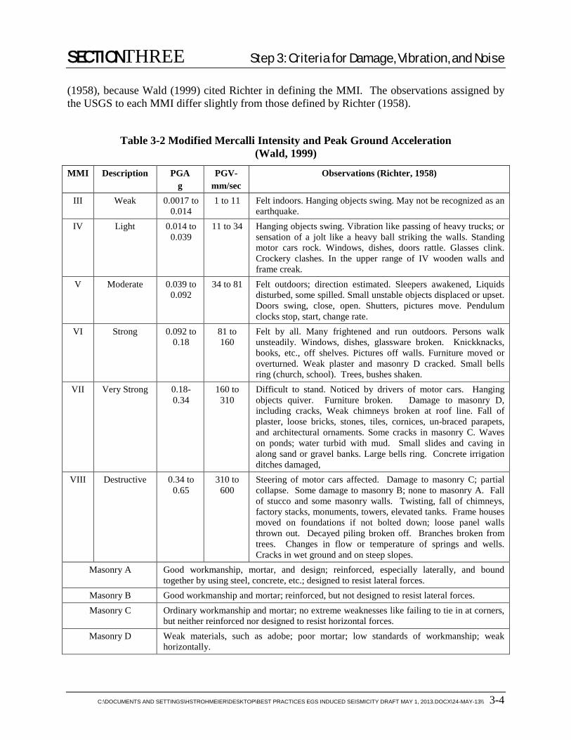
SECTIONTHREE Step 3: Criteria for Damage, Vibration, and Noise
C:\DOCUMENTS AND SETTINGS\HSTROHMEIER\DESKTOP\BEST PRACTICES EGS INDUCED SEISMICITY DRAFT MAY 1, 2013.DOCX\24-MAY-13\\ 3-4
(1958), because Wald (1999) cited Richter in defining the MMI. The observations assigned by the USGS to each MMI differ slightly from those defined by Richter (1958).
Table 3-2 Modified Mercalli Intensity and Peak Ground Acceleration (Wald, 1999)
MMI Description PGA g
PGV- mm/sec
Observations (Richter, 1958)
III Weak 0.0017 to 0.014
1 to 11 Felt indoors. Hanging objects swing. May not be recognized as an earthquake.
IV Light 0.014 to 0.039
11 to 34 Hanging objects swing. Vibration like passing of heavy trucks; or sensation of a jolt like a heavy ball striking the walls. Standing motor cars rock. Windows, dishes, doors rattle. Glasses clink. Crockery clashes. In the upper range of IV wooden walls and frame creak.
V Moderate 0.039 to 0.092
34 to 81 Felt outdoors; direction estimated. Sleepers awakened, Liquids disturbed, some spilled. Small unstable objects displaced or upset. Doors swing, close, open. Shutters, pictures move. Pendulum clocks stop, start, change rate.
VI Strong 0.092 to 0.18
81 to 160
Felt by all. Many frightened and run outdoors. Persons walk unsteadily. Windows, dishes, glassware broken. Knickknacks, books, etc., off shelves. Pictures off walls. Furniture moved or overturned. Weak plaster and masonry D cracked. Small bells ring (church, school). Trees, bushes shaken.
VII Very Strong 0.18-0.34
160 to 310
Difficult to stand. Noticed by drivers of motor cars. Hanging objects quiver. Furniture broken. Damage to masonry D, including cracks, Weak chimneys broken at roof line. Fall of plaster, loose bricks, stones, tiles, cornices, un-braced parapets, and architectural ornaments. Some cracks in masonry C. Waves on ponds; water turbid with mud. Small slides and caving in along sand or gravel banks. Large bells ring. Concrete irrigation ditches damaged,
VIII Destructive 0.34 to 0.65
310 to 600
Steering of motor cars affected. Damage to masonry C; partial collapse. Some damage to masonry B; none to masonry A. Fall of stucco and some masonry walls. Twisting, fall of chimneys, factory stacks, monuments, towers, elevated tanks. Frame houses moved on foundations if not bolted down; loose panel walls thrown out. Decayed piling broken off. Branches broken from trees. Changes in flow or temperature of springs and wells. Cracks in wet ground and on steep slopes.
Masonry A Good workmanship, mortar, and design; reinforced, especially laterally, and bound together by using steel, concrete, etc.; designed to resist lateral forces.
Masonry B Good workmanship and mortar; reinforced, but not designed to resist lateral forces. Masonry C Ordinary workmanship and mortar; no extreme weaknesses like failing to tie in at corners,
but neither reinforced nor designed to resist horizontal forces. Masonry D Weak materials, such as adobe; poor mortar; low standards of workmanship; weak
horizontally.

SECTIONTHREE Step 3: Criteria for Damage, Vibration, and Noise
C:\DOCUMENTS AND SETTINGS\HSTROHMEIER\DESKTOP\BEST PRACTICES EGS INDUCED SEISMICITY DRAFT MAY 1, 2013.DOCX\24-MAY-13\\ 3-5
The PGV limit shown for plaster-walled structures between 10 Hz and 40 Hz corresponds to a constant zero-to-peak (0-P) displacement limit of 0.2 mm (0.008 in). This is a relatively trivial displacement that structures should be able to tolerate, even though the associated peak ground acceleration at 40Hz is well above an MMI of VI. This suggests that the MMI scale is poorly correlated with PGV at spectral peaks above 10 Hz.
The USBM vibration limits shown in Figure 3-1 indicate a decreasing PGV (or PPV) limit with decreasing frequency below 2.5 Hz. This variation corresponds to a constant zero-to-peak (0-P) displacement curve of 0.8 mm (0.032 in). At these low frequencies, dynamic strains within buildings should be proportional to the ground acceleration rather than ground displacement. The USBM criteria for threshold damage are widely used for construction vibration and blasting vibration monitoring, but the constant displacement limit shown below 2.5 Hz is both puzzling and not well founded. A review of USBM RI 8507 suggests that the constant displacement below 2.5Hz is not clearly supported by measurement data or correlation of any such data with building damage. The USBM criterion curve is actually recommended as an “Alternative Blasting Level Criteria” in Appendix B of RI 8507, with the statement that “An ultimate maximum displacement of 0.030 inch (presumably zero-to-peak) is recommended, which would only be of concern where very low frequencies are encountered.” The report also reviews various literature concerning low frequency ground motion, such as by Thoenen and Windes (1942). However, Thoenen and Windes (1942) indicate that an acceleration limit of 0.1g is safe down to at least 2Hz. Other references referred to in USBM 8507 are discussed with reference to “low frequencies” that are not defined. No examples of threshold damage are presented for PGVs of less than 12.5 mm/sec (0.5 in/sec) at frequencies below 2.5Hz. Thus, applying the 0.8 mm (0.032 in) 0-P criterion at frequencies below 2.5 may be unreasonable, and, if so, would place severe and unnecessary restrictions on EGS-induced seismicity where such events would include low frequency ground motion. Rather, building damage criteria for ground motion of any kind at frequencies below roughly 2.5Hz should be based on experience with earthquake ground motions.
Accordingly, a composite building damage criterion curve is suggested in Figure 3-2 to address the inconsistancy between threshold cracking limits and seismological experience. The criterion is equivalent to the USBM RI 8507 criterion curve above 2.5 Hz. Below 2.5 Hz, the curve is drawn such that a constant acceleration of 0.02g with respect to frequency equates to the PGV criterion of 12.5mm/sec (0.5 in/sec) at 2.5 Hz. The criterion curve of 0.02 g, shown below 2.5 Hz, is comparable to an MMI of IV. The PGV criterion of 12.5mm/sec between 2.5 and 10 Hz also corresponds to an MMI of IV as indicated in Table 3-2. That is, the suggested threshold cracking criterion of Figure 3-2 is consistent with an MMI IV.
The modified curve thus rationalizes the MMI scale with the USBM RI 8507 building threshold damage criteria with some degree of conservatism. The minimum of 12.5 mm/sec (0.5 in/sec) of the curve between 2.5 and 10 Hz corresponds to the typical range of resonance frequencies of wood-frame structures. This curve is suggested as an appropriate PGV threshold cracking criterion for EGS-induced seismicity, one which is based on experience with seismic ground motion as well as mining- and construction-generated ground motions, and one which is generally considered conservative for a wide variety of wood-frame structures.

SECTIONTHREE Step 3: Criteria for Damage, Vibration, and Noise
C:\DOCUMENTS AND SETTINGS\HSTROHMEIER\DESKTOP\BEST PRACTICES EGS INDUCED SEISMICITY DRAFT MAY 1, 2013.DOCX\24-MAY-13\\ 3-6
Figure 3-1. USBM RI 8507 (1980) Vibration Limits for Threshold Cracking and MMI
Curves
1
10
100
1000
1 10 100
PGV
- MM
/SEC
FREQUENCY - Hz
19 mm/sec (Drywall)
12.5mm/sec (Plaster)
50 mm/sec
Constant Displacement0.2 mm 0-P
Constant Displacement0.8 mm 0-P
0.2g (MMI VII)
0.1g (MMI VI)
0.05g (MMI V)
0.025g (MMI IV)

SECTIONTHREE Step 3: Criteria for Damage, Vibration, and Noise
C:\DOCUMENTS AND SETTINGS\HSTROHMEIER\DESKTOP\BEST PRACTICES EGS INDUCED SEISMICITY DRAFT MAY 1, 2013.DOCX\24-MAY-13\\ 3-7
Figure 3-2. Composite Building Threshold Cracking Criteria based on USBM RI 8507
(1980) and MMI Scale
1
10
100
1000
1 10 100
PGV
- MM
/SEC
FREQUENCY - Hz
50 mm/sec
0-PDisplacement0.2 mm
PGA = 0.02g (MMI IV)
12.5 mm/sec (MMI IV)

SECTIONTHREE Step 3: Criteria for Damage, Vibration, and Noise
C:\DOCUMENTS AND SETTINGS\HSTROHMEIER\DESKTOP\BEST PRACTICES EGS INDUCED SEISMICITY DRAFT MAY 1, 2013.DOCX\24-MAY-13\\ 3-8
The threshold damage criterion is given as a function of frequency, for which an estimate of the spectral peak associated with the PGV is needed. The determination of the spectral peak of the PGV is typically made by counting “zero-crossings” of the velocity motion. This method is subject to some interpretation where the velocity waveforms contain substantial high frequency content, but it is widely used in the blasting and construction industry. More sophisticated techniques apply Fourier analysis to the transient velocity waveform to define the spectral peak. The quantity plotted in Figure 3-2 against the criterion curve is the magnitude of the velocity waveform along the vertical axis and the spectral peak along the horizontal axis.
Neglecting the maximum permissible PGV at 40Hz and higher frequencies (50mm/sec), one may simply determine the vector-sum PGA, PGV and zero-to-peak (0-P) ground displacement by differentiation and integration of the velocity waveforms. If all three of these amplitudes exceed, respectively, 0.02g, 12.5mm/sec, and 0.2mm 0-P (0.4 mm P-P), then the event would be in excess of the suggested threshold cracking criterion, regardless of the spectrum. If any one or more of these peak amplitudes did not exceed its respective threshold, then the ground motion might be within the threshold cracking limit. This would be a less-than-conservative test, but would not require determination of a spectral peak by counting zero-crossings or Fourier analysis, thus simplifying real-time data analysis and interpretation. Additional investigation of this technique is needed. High amplitude PGV’s at spectral peak frequencies in excess of 40Hz are likely to be rare. However, if this does occur, then an additional criterion would be a maximum PGV of 50mm/sec if the 0-P displacement is less than 0.2 mm, respectively. Adjustment of these acceleration, velocity, and displacement thresholds might be appropriate, based on a review of seismic waveforms and local building types. However, distinction between building types (for example, wood frame or masonry) is usually not made when applying criteria.
Figure 3-3 is an example output of an Instantel Minimate blast vibration monitor that illustrates the velocity waveform and PGVs plotted against the USBM criteria. This chart is typical of the type of output that is used for monitoring blasting- and construction-related transients as well as continuous vibration. The PGVs in three orthogonal axes are listed, together with the vector sum. The peak vector sum indicates the maximum PGV in any direction. This type of display can be used for assessing EGS-induced seismicity, though the modified criterion curve of Figure 3-2 is suggested here in lieu of the USBM RI 8507 criteria shown in Figure 3-1 and Figure 3-3.

SECTIONTHREE Step 3: Criteria for Damage, Vibration, and Noise
C:\DOCUMENTS AND SETTINGS\HSTROHMEIER\DESKTOP\BEST PRACTICES EGS INDUCED SEISMICITY DRAFT MAY 1, 2013.DOCX\24-MAY-13\\ 3-9
Figure 3-3. Example Event Report
SECTIONTHREE Step 3: Criteria for Damage, Vibration, and Noise
C:\DOCUMENTS AND SETTINGS\HSTROHMEIER\DESKTOP\BEST PRACTICES EGS INDUCED SEISMICITY DRAFT MAY 1, 2013.DOCX\24-MAY-13\\ 3-10
3.2.2 Minor and Major Damage Dowding (1996) summarizes work by Edwards and Northwood (1960) and Northwood et al (1963), who characterize minor and major damage. Minor damage would include superficial damage not causing weakening of the structure, but would include broken windows, loosened or fallen plaster, and hairline cracks in masonry. Minor damage would be associated with a moderate earthquake of MMI VI or higher. Major damage would include serious weakening of the structure. This would be indicated by the presence of large cracks or shifting of the foundation or bearing walls, or major settlement resulting in distortion or weakening of the superstructure. Dowding (1985) indicates that threshold cracking occurred in older structures at about 76 mm/sec (3 in/sec), minor damage at 114 mm/sec (4.5 in/sec), and major damage at 203 mm/sec (8 in/sec). The spectral frequencies associated with these damages were not identified. From these examples, a reasonable criterion for major damage would be 125 mm/sec (5 in/sec). However, damage at lower amplitudes of PGV may occur, and would depend on the quality of construction, age, condition, etc. For example, unreinforced masonry structures may be more prone to structural damage than modern reinforced masonry structures. Construction vibration damage criteria for historical structures are generally lower or more restrictive than those of modern structures, even though historical structures may easily withstand substantially greater motion than modern structures of the same type.
Minor and major damage to residential, wood frame, and masonry structures should be nil if EGS seismicity remains within threshold cracking criteria. Hazard and risk assessment methods are described in Sections 5 and 6, respectively.
3.3 DAMAGE CRITERIA FOR CIVIL STRUCTURES Civil structures include the following:
Dams
Bridges
Highways
Railroads
Tunnels
Power Plants
Pipe Lines
Runways
Damage criteria for civil structures would depend on the nature of the structure. Modern civil structures are by regulation designed to withstand substantial earthquake ground motions. Ground motions induced by EGS activities are not expected to exceed those of natural origin in seismically active areas. Hence, damage due to EGS seismicity would not be expected to damage civil structures such as those listed above if they are designed to seismic codes for seismic areas. The construction design drawings and specifications should be reviewed for seismic design criteria that may be applicable to EGS seismicity. However, seismic criteria may be defined in

SECTIONTHREE Step 3: Criteria for Damage, Vibration, and Noise
C:\DOCUMENTS AND SETTINGS\HSTROHMEIER\DESKTOP\BEST PRACTICES EGS INDUCED SEISMICITY DRAFT MAY 1, 2013.DOCX\24-MAY-13\\ 3-11
terms of acceleration, and are probably excessively conservative for frequencies above 10Hz. (See the discussion above regarding Figure 3-2.)
3.4 DAMAGE CRITERIA FOR BURIED STRUCTURES The estimate of probable damage to buried structures is based on the strain induced by the passing seismic shear wave and the strength of the material forming the structure. The strains due to passing shear waves in buried structures can conservatively be assumed to be the same as those of the surrounding soil. Buried structures are not subject to resonance amplification in the same manner as a building, due to the loading of the soil and damping related to re-radiation of waves into the soil by the structure. Thus, buried structures should withstand much higher ground motion amplitudes than those that would damage surface structures.
Dowding (1996) discusses vibration damage to buried structures in some detail. The probability of damage should be based on expected maximum ground strains and the flexibility of the buried structures, which may require finite-element analysis. In any case, EGS seismicity that would not cause cosmetic damage to surface structures would very likely not damage underground structures.
3.4.1 Wells Dowding (1996) describes results obtained from a USBM study concerning water wells. The study indicated no loss of well capacity with PGVs produced by blasting as high as 84 mm/sec (3.3 in/sec) and no loss of water level with PGVs as high as 141 mm/sec (5.5 in/sec). This does not stop well owners from claiming that construction-related vibration damages their wells. Thus, inspection of deep water wells prior to project implementation should be conducted to assess well condition prior to EGS stimulation. This pertains to ground motions; dewatering or changes to aquifers are another matter to be considered by others.
3.4.2 Pipelines Failure of gas transmission lines due to weld failures and other defects are of concern with respect to pipeline operations. Relatively large tensile hoop stresses in the pipe wall due to high pressure gas would be superposed with strains induced by passing ground motion waves. Old pipelines, especially those manufactured with welded seams, have some history of rupturing under excessive pressure. However, a properly maintained and designed pipeline should offer substantial margin of safety against normal soil movement over time with resulting strains in the soil that may exceed those associated with passing low amplitude seismic waves from induced seismicity.
Assuming a shear-wave velocity in soil of 200 m/sec and PGV of perhaps 0.25 m/sec (10 in/sec), the peak strain in the soil due to the passing wave would be on the order of 0.25/200 = 0.00125, giving a stress in the pipeline wall of 260 MPa (37,500 psi), comparable with the yield strength of mild steel. Designing an EGS project to limit PGVs to threshold damage criteria on the order of 50 mm/sec (2 in/sec) would give a peak stress in the steel of 22 MPa (7,500 psi), well within the yield strength of mild steel. Dynamic stresses in the pipe wall should be less, due to the higher modulus of the steel relative to that of the soil, though a complete analysis would include the stresses due to pressurization.

SECTIONTHREE Step 3: Criteria for Damage, Vibration, and Noise
C:\DOCUMENTS AND SETTINGS\HSTROHMEIER\DESKTOP\BEST PRACTICES EGS INDUCED SEISMICITY DRAFT MAY 1, 2013.DOCX\24-MAY-13\\ 3-12
Dowding (1996) describes pipe wall strain measurements conducted during blasting at short range. PGVs on the order of 1.14 m/sec (45 in/sec) produced strains in the pipe wall on the order of 500E-6, giving a pipe wall stress on the order of 100 MPa (15,000 psi). Scaling down to PGVs on the order of 5 in/sec would imply a pipe wall stress of 12 MPa (1,700 psi), a relatively small amount. Again, the seismically induced stresses must be combined with operating pipeline wall stresses due to pressure.
As with any civil structure, pipelines would be expected to be constructed to meet large ground motion seismic criteria. Pipeline plan and profile drawings, operating pressures, and fluid types should be reviewed and discussed with the pipeline operator. Gas transmission lines in poor condition should be identified and considered carefully. Inspection of any nearby gas transmission line may be considered prior to EGS startup.
3.4.3 Basement Walls Basement walls are usually constructed of either concrete block or reinforced concrete. Dowding (1996) indicates that the former exhibited cracking of mortar joints at 75 mm/sec (3 in/sec). Reinforced concrete walls cracked when the PPV exceeded 250 mm/sec (10 in/sec), though in this case the failure was at the juncture of two walls.
Again, EGS projects designed to limit PPV or PGV to threshold cracking criteria should cause no cracking of basement walls. The existing conditions of basement walls and structures should be documented with pre-construction surveys prior to EGS stimulation.
3.4.4 Tunnels Dowding and Rozen (1978) summarize damages to tunnel structures of various types caused by earthquakes. The summary considers 71 tunnel structures and 13 different earthquakes with Richter magnitudes ML 5.8 to 8.3 and with focal depths ranging from 13 to 40 km. The review included four types of tunnels; (a) unlined rock tunnels; (b) temporary steel liners with wood blocking; (c) final concrete lining; and (d) final masonry lining. The conclusions are
(1) Tunnels are less prone to seismic damage than surface structures for a given surface ground motion
(2) No damage to tunnels of any type occurred for estimated ground surface PGVs of 0.2 m/sec (8 in/sec) and PGAs of 0.19 g
(3) In cases where shaking was identified as causing tunnel damage, the tunnels were in ground or rock of poor condition
(4) Total collapse of a tunnel was found only in cases of an intersecting fault, and
(5) Tunnels are much safer than surface structures for the same intensity of shaking.
However, the estimated ground motions are for the ground surface, and lower amplitudes of ground motion likely occurred at tunnel depth. Some amplification of tunnel stresses might occur for seismic wavelengths comparable with the tunnel diameter. Tunnels in soil with liquefaction potential or tunnel portals near landslide-prone areas, or tunnels intersected by faults or poor soil or rock conditions, are at greater risk than tunnels in competent rock or tunnels with concrete liners and grouted soil. Tunnels within an EGS seismic zone should be identified and reviewed with the responsible agencies to determine damage potential. A survey of any such tunnels
SECTIONTHREE Step 3: Criteria for Damage, Vibration, and Noise
C:\DOCUMENTS AND SETTINGS\HSTROHMEIER\DESKTOP\BEST PRACTICES EGS INDUCED SEISMICITY DRAFT MAY 1, 2013.DOCX\24-MAY-13\\ 3-13
should be conducted as part of the EGS impact assessment. Tunnels may include (but not be limited to) railroad, highway, mining or water transport tunnels. Tunnels should be inspected prior to EGS activities to identify pre-existing defects, cracks, seepage, etc.
3.5 LANDSLIDE AND ROCKSLIDE Landslides and rockslides caused by ground motion are difficult to predict, though they have been documented in the case of large earthquakes. Landslides may involve very slow movement of soil over time, or may be abrupt, as with an avalanche. Rock slides may involve an avalanche of rock, or the occasional motion of rocks or boulders that, after a period of time, result in the accumulation of rock mounts and slopes.
Loose rock, such as talus slopes, may be viewed as colluvium deposited at its angle of repose. Ground motions associated with blasting are usually too small to cause landslides of colluvium. However, the potential for rockslide in response to ground motion exists. This is of particular interest to highway construction engineers for blasting at the base of talus slopes. Landslide triggering associated with strong-motion seismic events of the order of M 6 or higher is discussed by Wieczorek (Transportation Research Board, 1996). Evidently, landslide triggering by smaller events is relatively rare. Historical seismicity should define an acceptable limit for PGVs associated with EGS.
3.6 HUMAN RESPONSE Human response to ground vibration includes perceptible vibration and low frequency ground-borne noise, one or both of which are common with rail transportation, construction, and mining operations. Some of the substantial literature that exists for human response to floor vibration and ground-borne noise caused by these sources is applicable to transient induced seismicity, specifically that regarding mining and construction activities. Evidently, both ground motion and ground-borne noise from EGS activity near Basel, Switzerland has caused human annoyance, and the literature regarding this should be consulted. Criteria for assessing the significance of vibration and ground-borne noise are discussed below.
3.6.1 Third Octave Filters Third octave filters are commonly used for assessing human response to both noise and vibration. (Third octave filters are also used for describing the vibration tolerance of sensitive instrumentation, as discussed below.) A third octave filter is a unity-gain filter with a bandwidth of approximately 23% of its nominal center frequency. The third octave filter response is “maximally flat” with, typically, a 6-pole filter roll-characteristic of 36dB per octave outside of the filter pass-band. Third octave filters are normally provided with high quality commercial sound level meters or vibration analyzers, and can be used in a practical manner for monitoring of ground motions. The responses of third octave filters are specified in ANSI Standard S1.11-2004 (R2009).
The response time of a third octave filter increases with its order, and is inversely proportional to its bandwidth. That is, the response time of 6th order filter is longer than the response time of a 3rd order filter. Older analog third octave filters were usually 3rd order, and referred to as Class III filters in the ANSI standards. Modern digital sound and vibration meters almost universally provide 6th order filters. The response time is important for short-period transient events such as

SECTIONTHREE Step 3: Criteria for Damage, Vibration, and Noise
C:\DOCUMENTS AND SETTINGS\HSTROHMEIER\DESKTOP\BEST PRACTICES EGS INDUCED SEISMICITY DRAFT MAY 1, 2013.DOCX\24-MAY-13\\ 3-14
those produced by induced seismicity. A third octave filter with center frequency of 4 Hz will have a filter bandwidth of slightly less than 1-Hz, with a corresponding response time of the order of one second. Induced seismic events by EGS projects will likely have durations less than one second. The averaging time used for measuring the root-mean-square vibration needs to be long enough to include the filter response time. The vibration “dose” analysis approach discussed below is intended to circumvent this issue.
3.6.2 Vibration
Metrics ISO 2631-1 (1997) is a standard for assessing human response to acceleration for people standing, sitting, or lying. Frequency weightings are specified for application to third octave vibration acceleration spectra extending from 0.5 to 80 Hz, together with methods for combining the weighted acceleration in all six degrees of freedom.
Two procedures are recommended in ISO 2631-1 for assessing transient acceleration: the running RMS evaluation method and the fourth-power dose method. The running RMS method involves determining the RMS amplitude of the weighted acceleration continuously with an integration time of one second. Exponential weighting with respect to time may be employed. The maximum RMS amplitude occurring during a transient event is called the Maximum Transient Vibration Value (MTVV).
The fourth-power vibration dose is defined as the fourth root of the integral with respect to time of the weighted acceleration amplitude raised to the fourth power. This approach is intended to represent the peak value within a given time period.
Siskind et al. (1980) suggest using a second-power vibration velocity dose computed by integrating the square of the vibration velocity amplitude over the entire signature with respect to time. As with the fourth power approach, this method is also independent of the integration time.
The integration times used in the dose procedures must be short enough to avoid introduction of background vibration into the estimate. In the absence of background vibration, the result would be independent of the integration time, provided that the integration time covers or spans the duration of the transient event.
The second-power dose approach may be used with virtually any good quality sound level meter or vibration analyzer, and the results should be comparable with the ISO 2631 fourth-power dose. Some sound level meters or vibration analyzers can measure the fourth-power dose.
ISO 2631-2 (2003) recommends limits for human exposure to vibration in buildings using the measurement methods outlined in the ISO 2631-1 standard. The standard recommends a single weighting network or filter to be applied to analog ground acceleration to obtain the weighted acceleration regardless of the axis of vibration. The filter is a simple low-pass filter with corner frequency of 5.6 Hz, giving a constant acceleration response below 5.6 Hz, and a constant velocity response above 5.6 Hz. Band limiting filters are also recommended, with corner frequencies of 0.8Hz (high pass) and 100 Hz (low pass) to define the overall bandwidth. The filter response is tabulated at third octave band center frequencies for application to third octave acceleration data. The 0.8 Hz high pass and 100 Hz low pass filters are probably unnecessary, as

SECTIONTHREE Step 3: Criteria for Damage, Vibration, and Noise
C:\DOCUMENTS AND SETTINGS\HSTROHMEIER\DESKTOP\BEST PRACTICES EGS INDUCED SEISMICITY DRAFT MAY 1, 2013.DOCX\24-MAY-13\\ 3-15
the spectral peak of EGS seismic acceleration and velocity associated with induced seismicity by EGS projects would likely be between 1 Hz and 100 Hz.
ANSI S2.71-1983 (R2006) recommends third octave acceleration and velocity base-response curves for characterizing human response to vibration, referring to ANSI S3.18-1979. The third octave acceleration and velocity base-response curves are plotted in Figure 3-4 and Figure 3-5, respectively. The base-response curves are approximately twice the threshold of perception. Base-response curves are provided for each axis, and a composite curve is also recommended. (ANSI S3.18-1979 is no longer in publication as of this writing, supplanted by ANSI S2.72-1, which primarily follows ISO 2631-1.) A simple (single-pole) low-pass filter response function is recommended in ANSI S2.71 for filtering analog acceleration data, equivalent to the weighting function recommended in ISO 2631-2 (2003), but without band limiting filters at 0.8 and 100Hz. The corresponding filter for analog velocity data would be a (single-pole) high-pass filter with corner frequency of 5.6Hz. The ANSI S2.71 standard suggests that the root-mean-square (RMS) amplitude should be determined over the duration of the transient, which, for EGS seismicity, would typically be of the order of a second or less.

SECTIONTHREE Step 3: Criteria for Damage, Vibration, and Noise
C:\DOCUMENTS AND SETTINGS\HSTROHMEIER\DESKTOP\BEST PRACTICES EGS INDUCED SEISMICITY DRAFT MAY 1, 2013.DOCX\24-MAY-13\\ 3-16
1
10
100
1000
1 10 100
Z-AXIS ACCELX,Y AXIS ACCELCOMBINED-AXIS ACCEL
1/3
OC
TAVE
RM
S A
CC
ELER
ATI
ON
FREQUENCY - HZ
100 g
101010
1
mm/sec2
0.1
Figure 3-4. Base Response Limits for Whole-Body Third-Octave Acceleration Exposure –
Derived from ANSI S2.71

SECTIONTHREE Step 3: Criteria for Damage, Vibration, and Noise
C:\DOCUMENTS AND SETTINGS\HSTROHMEIER\DESKTOP\BEST PRACTICES EGS INDUCED SEISMICITY DRAFT MAY 1, 2013.DOCX\24-MAY-13\\ 3-17
Figure 3-5. Base Response Limits for Whole-Body Third-Octave Velocity Exposure –
Derived from ANSI S2.71
0.1
1
1 10 100
Z-AXIS VELOCX,Y-AXIS VELOCICOMBINED-AXIS VELOC
1/3
OCT
AVE
RM
S VE
LOCI
TY -
MM
/SEC
FREQUENCY - HZ

SECTIONTHREE Step 3: Criteria for Damage, Vibration, and Noise
C:\DOCUMENTS AND SETTINGS\HSTROHMEIER\DESKTOP\BEST PRACTICES EGS INDUCED SEISMICITY DRAFT MAY 1, 2013.DOCX\24-MAY-13\\ 3-18
Examples Figure 3-6 illustrates two example seismograms. One is the un-weighted ground surface acceleration (measured in one particular axis), and the other is the weighted acceleration obtained by low-pass filtering the acceleration with a single-pole (6 dB attenuation per octave) filter with corner frequency of 5.6Hz as recommended in ANSI S2.71. The peak amplitude of the weighted acceleration signal is less than the PGA by only a modest amount, as much of the spectrum of the acceleration signature is above the corner frequency of 5.6Hz. A shorter period acceleration transient with higher frequency content would produce a significantly lower weighted acceleration waveform.
Third octave spectra of the un-weighted acceleration are plotted in Figure 3-7. The acceleration spectra are the peak, the fourth-power dose, the second power dose, and the MTVV of the third octave band filtered signals. The corresponding values for the overall (broadband, un-weighted) PGA, the overall fourth-power acceleration dose, the overall second acceleration dose, and the overall MTVV are plotted at the left hand side of Figure 3-7. The corresponding weighted peak acceleration, the weighted fourth-power acceleration dose, the weighted second-power dose, and the weighted MTVV are plotted at the right-hand side.
The fourth-power and the second-power dose curves are almost indistinguishable from one another, suggesting that either the second-power acceleration dose approach or the fourth-power dose may be used for characterizing this particular transient ground motion. The peak values of the overall and weighted acceleration are roughly about 50% to 100% higher than either of the dose magnitudes. The MTVV (the maximum root-mean-square amplitude determined over any one-second time period) is generally significantly less than the dose magnitudes. This makes the dose approach most attractive for event characterization relative to human response. However, the dose units include the square root of or fourth root of time, and thus differ from the MTVV units, which is a root-mean-square acceleration.
The third octave analyses indicate that the acceleration dose is between 64 and 128 times the ANSI S2.71 base response curve, and thus highly perceptible to humans. The peak third octave acceleration is plotted for illustration, but should not necessarily be used for comparison with the ANSI S2.71 base response curve, as these specifically apply to RMS third octave acceleration or dose. Even so, the peak values are not much greater than the dose values.
The spectrum of this particular seismogram is such that its peak occurs at the transition frequency between constant acceleration and constant velocity regions of the ANSI curves. As a result, employing only the acceleration or velocity for assessing human annoyance potential is not entirely adequate. However, filtering the acceleration signal with a 5.6-Hz low pass filter as recommended in ANSI S2.71 and ISO 2631-2 provides a single number of weighted acceleration for assessing human annoyance potential. The weighted accelerations are plotted at the right hand side of Figure 3-7.
Measurement Location The ISO 2631-2 and ANSI S2.71 standards recommend measuring vibration acceleration (or velocity) in the buildings in which people would be located. This may be impractical for EGS monitoring activity, and would be difficult from a prediction point of view, because building
SECTIONTHREE Step 3: Criteria for Damage, Vibration, and Noise
C:\DOCUMENTS AND SETTINGS\HSTROHMEIER\DESKTOP\BEST PRACTICES EGS INDUCED SEISMICITY DRAFT MAY 1, 2013.DOCX\24-MAY-13\\ 3-19
response may vary considerably from one to the next. The most practical approach for both prediction and monitoring would be to use the ground surface acceleration.
Sidewalks and asphalt surfaces are ideal measurement surfaces for monitoring EGS vibration, as the sidewalk has a large bearing surface relative to its mass, assuming intimate contact between sidewalk and soil. Transducers buried in pits at a depth of at most 1 m provide excellent permanent monitoring points. However, the back-fill of the pit must be of the same density as the surrounding soil. That is, the transducers should not be encased in concrete blocks that are in turn buried in the soil, as the massive concrete block and soil will act as a spring-mass isolation system with a damped resonance of the order of perhaps 10 to 30Hz. This may be acceptable for strong-motion seismicity with spectral peak at 3Hz, but could be problematic for high spectral peak events.
From a practical point of view, the building interior floor vibration acceleration or velocity will be roughly one to two times the exterior ground surface velocity or acceleration. This comparison may be the result of measuring too closely to the foundation of the building, as the ground surface response is reduced by the presence of the building foundation. Considerable uncertainty exists in characterizing building response to vibration, and, considering the large number of building types and people that may be present near an EGS project, the better approach would be to estimate a reasonable amplification factor that is representative of the buildings in the area. In the absence of more information, one may simply take the ground surface incident acceleration as a first estimate, especially for transient motions with spectral peaks at frequencies below the fundamental floor resonance frequencies of structures. These fundamental frequencies are usually of the order of 12Hz or higher for residential wood frame structures. The incident ground surface acceleration or velocity can be multiplied by a factor of two if an additional safety factor is desired.

SECTIONTHREE Step 3: Criteria for Damage, Vibration, and Noise
C:\DOCUMENTS AND SETTINGS\HSTROHMEIER\DESKTOP\BEST PRACTICES EGS INDUCED SEISMICITY DRAFT MAY 1, 2013.DOCX\24-MAY-13\\ 3-20
Figure 3-6. Example Ground Acceleration
-0.06
-0.04
-0.02
0
0.02
0.04
0.06
10 11 12 13 14 15TIME - SEC
AC
CEL
ERA
TIO
N -
G
ACCELERATION
WEIGHTED ACCELERATION

SECTIONTHREE Step 3: Criteria for Damage, Vibration, and Noise
C:\DOCUMENTS AND SETTINGS\HSTROHMEIER\DESKTOP\BEST PRACTICES EGS INDUCED SEISMICITY DRAFT MAY 1, 2013.DOCX\24-MAY-13\\ 3-21
Figure 3-7. Comparison of third octave acceleration spectra with ANSI S2.71 Base
Response curves and Multiples Thereof
0.001
0.01
0.1
1
10
OA 1 2 4 8 16 31.6 63 ANSI-S2.71FREQUENCY - HZ
AC
CEL
ERA
TIO
N
PEAK 1/4 ROOT-SUM-QUAD-DTROOT-SUM-SQUARE-DT MAXIMUM RMS - MTVVBASE RESPONSE x 64 BASE RESPONSE x 32BASE RESPONSE x 16 BASE RESPONSE x 8BASE RESPONSE x 4 BASE RESPONSE x 2BASE RESPONSE
1
0.1
m/sec2
0.01
0.001
g
SECTIONTHREE Step 3: Criteria for Damage, Vibration, and Noise
C:\DOCUMENTS AND SETTINGS\HSTROHMEIER\DESKTOP\BEST PRACTICES EGS INDUCED SEISMICITY DRAFT MAY 1, 2013.DOCX\24-MAY-13\\ 3-22
Recommended Practice for Assessing Human Response to EGS Vibration The ISO 2631-1, ANSI S2.71, and ANSI S2.71 standards provide excellent guidelines for assessing building interior floor vibration. Of the various methods, the recommended approach is to employ a second-power acceleration dose method with a good quality precision integrating sound level meter or vibration meter, or the fourth-power dose method as recommended by ISO 2631-1. As shown above, the second-power dose method gives results that are very similar to the fourth-power acceleration dose method for transient events of the order of one second or less. In the event that a transient duration extends several seconds, both the second-power and fourth-power dose methods will reflect the effect of increasing transient duration.
ANSI S2.71 Acceleration
Examples of limits for third octave acceleration dose are listed in Table 3-3 in terms of multiples of the composite base response curve given in ANSI S2.71. The base response curve corresponds to third octave acceleration and velocity limits of 0.00036 g and 100 micron/sec (0.1 mm/sec) for frequencies below and above 5.6 Hz, respectively. These limits would be applied to third octave vibration acceleration dose as described above. The composite acceleration base response curve is illustrated in Figure 3-4, and the corresponding composite third octave velocity base response curve is illustrated in Figure 3-5. Third octave acceleration data are plotted against these criteria curves in Figure 3-7. The dose responses shown in Figure 3-7 fall between 32 and 64 times the base response curve.
The prototype limits are given as a function of recurrence interval. Thus, events that recur over time periods of less than 10 minutes during the night would be acceptable provided that their third octave acceleration dose was within the base response curve. Events recurring over a time period of less than one hour but not less than 10 minutes during the night would be acceptable if their acceleration doses were within twice the base response curve. These limits would be multiplied by a factor of two for daytime periods. The daytime limits are extended in multiples of two for larger time periods. However, the ability to control or predict the time of day during which an induced seismic event occurs is severely limited. Therefore, the night time limits should probably be applied as a conservative measure. A maximum limit of 64 times the base the response curve is suggested, as this would correspond to an RMS magnitude of 0.023 g with a PGA of perhaps 0.05 g (MMI V) and would exceed the threshold cracking criterion.
The limits listed in Table 3-3 may require adjustment based on hazard assessment accuracy, practicality, receiver type, land use, etc. A similar table may be developed for hospitals, nursing homes, schools, and other land uses where vibration may interfere with activity. Also, higher limits might be considered during EGS stimulation over a short period of time, with more restrictive post-stimulation limits for production over much longer time periods, though such an approach must be vetted with stakeholders.
Weighted Acceleration Dose Limits
The single number weighted acceleration approach is recommended to reduce the complexity of assessing human response to ground motion. As indicated above, this involves filtering the acceleration signal with a low pass single-pole filter with roll-off frequency of 5.6Hz, as recommended in ANSI S2.71. The weighted acceleration should then be squared and integrated with respect to time over the transient duration. The results should be summed over each axis, and the square root of the sum should be taken to obtain the composite vector-sum dose. This

SECTIONTHREE Step 3: Criteria for Damage, Vibration, and Noise
C:\DOCUMENTS AND SETTINGS\HSTROHMEIER\DESKTOP\BEST PRACTICES EGS INDUCED SEISMICITY DRAFT MAY 1, 2013.DOCX\24-MAY-13\\ 3-23
process will generally yield a higher value that would be obtained by comparison of third octave spectra with the response curves.
Prototype limits for weighted composite acceleration dose are listed in Table 3-4. The prototype acceleration limits are derived by taking the multiple of the base response curve acceleration limit at the low frequency limit (below 5.6Hz) and multiplying by the square root of two (+3dB). Thus, the low frequency acceleration limit for the ANSI S2.71 acceleration base response curve at 2Hz is 0.00036 g, and multiplying by 1.4 gives a weighted acceleration limit of 0.0005 g. The factor of root two is intended to accommodate the difference between the weighted acceleration and the maximum value obtained in any third octave band, which is necessarily less than the weighted acceleration. (A more conservative and acceptable approach would be to not employ the factor of 1.4.)
An event with maximum weighted acceleration dose of 0.0005 g would be largely unnoticed. Events of this nature would correspond to a weighted velocity of about 100 micron/sec, typically considered as a threshold impact on human occupancy, though the threshold of human perception is actually less than this by perhaps a factor of two. (ANSI Standard S2.71.) Events of this type could occur repeatedly throughout the night without generating significant annoyance. A weighted acceleration dose of 0.001g occurring repeatedly through the day time period would probably be acceptable for daytime residential occupancy. However, above these dose amplitudes, human annoyance may rise rapidly. Repeated exposure to perceptible vibration with high occurrence rate (short recurrence period) would likely generate significant reaction. A maximum dose of 0.032 g-sec1/2 or 0.032 g-sec1/4 is suggested, as the PGA associated with such an even would be 0.05 g or 0.06 g, corresponding to an MMI V, and could be above the threshold cracking criterion of 0.02g.
Weighted Velocity Dose Limits
Table 3-5 contains prototype vibration dose limits that correspond to the prototype limits given in Table 3-4. The weighted vibration velocity would be obtained by applying a high-pass single-pole filter with corner frequency of 5.6 Hz to the velocity waveform. This may be most appropriate for velocity data obtained with a 1-Hz or 2-Hz seismometer or geophone. Typical EGS vibration is expected to have most of its energy at frequencies below 10 Hz. Thus, either the weighted velocity or the weighted acceleration are probably of equal merit. The choice may depend more on transducer selection and instrumentation simplicity.
PGA and PGV Limits
Detailed prediction of EGS ground acceleration or velocity signatures with spectral content is perhaps impracticable, whereas prediction of the PGA or PGV may be straight-forward given appropriate EGS seismic models and statistics. Thus, human annoyance may have to be based on PGA and PGV, rather than weighted RMS or dose acceleration. In this case, the PGA and PGV would be about 50% to 100% higher than the un-weighted acceleration or velocity dose, judging from the results given in Figure 3-7. If spectral characteristics can be predicted, the weighted peak acceleration can be estimated, in which case the prototype limits would be roughly 50% to 100% higher than the prototype limits shown for the weighted acceleration dose in Table 3-4 or the weighted velocity dose limits given in Table 3-5.
If the joint probability of recurrence of an event with given un-weighted PGA and PGV can be predicted, then the PGA and PGV may be compared directly with the limits given in Table 3-4
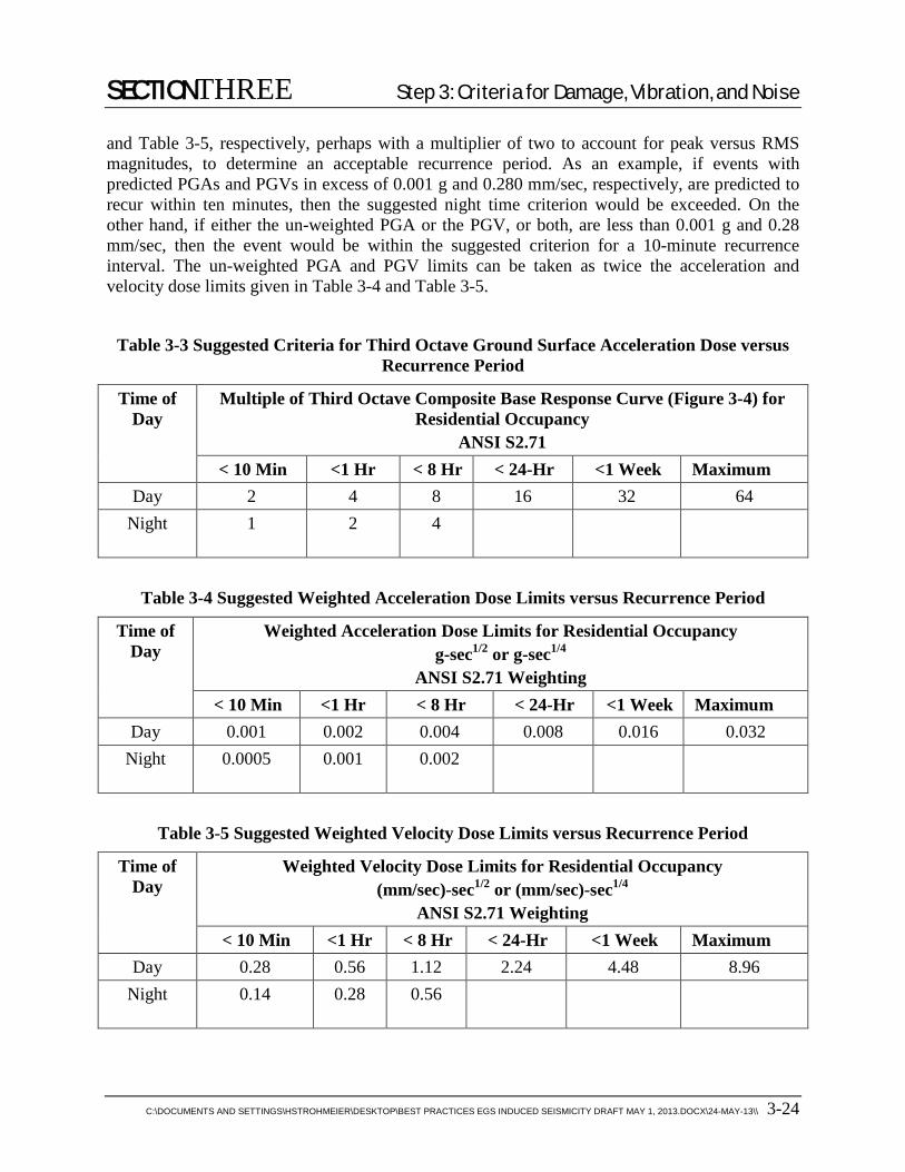
SECTIONTHREE Step 3: Criteria for Damage, Vibration, and Noise
C:\DOCUMENTS AND SETTINGS\HSTROHMEIER\DESKTOP\BEST PRACTICES EGS INDUCED SEISMICITY DRAFT MAY 1, 2013.DOCX\24-MAY-13\\ 3-24
and Table 3-5, respectively, perhaps with a multiplier of two to account for peak versus RMS magnitudes, to determine an acceptable recurrence period. As an example, if events with predicted PGAs and PGVs in excess of 0.001 g and 0.280 mm/sec, respectively, are predicted to recur within ten minutes, then the suggested night time criterion would be exceeded. On the other hand, if either the un-weighted PGA or the PGV, or both, are less than 0.001 g and 0.28 mm/sec, then the event would be within the suggested criterion for a 10-minute recurrence interval. The un-weighted PGA and PGV limits can be taken as twice the acceleration and velocity dose limits given in Table 3-4 and Table 3-5.
Table 3-3 Suggested Criteria for Third Octave Ground Surface Acceleration Dose versus Recurrence Period
Time of Day
Multiple of Third Octave Composite Base Response Curve (Figure 3-4) for Residential Occupancy
ANSI S2.71 < 10 Min <1 Hr < 8 Hr < 24-Hr <1 Week Maximum
Day 2 4 8 16 32 64 Night 1 2 4
Table 3-4 Suggested Weighted Acceleration Dose Limits versus Recurrence Period
Time of Day
Weighted Acceleration Dose Limits for Residential Occupancy g-sec1/2 or g-sec1/4
ANSI S2.71 Weighting < 10 Min <1 Hr < 8 Hr < 24-Hr <1 Week Maximum
Day 0.001 0.002 0.004 0.008 0.016 0.032 Night 0.0005 0.001 0.002
Table 3-5 Suggested Weighted Velocity Dose Limits versus Recurrence Period
Time of Day
Weighted Velocity Dose Limits for Residential Occupancy (mm/sec)-sec1/2 or (mm/sec)-sec1/4
ANSI S2.71 Weighting < 10 Min <1 Hr < 8 Hr < 24-Hr <1 Week Maximum
Day 0.28 0.56 1.12 2.24 4.48 8.96 Night 0.14 0.28 0.56

SECTIONTHREE Step 3: Criteria for Damage, Vibration, and Noise
C:\DOCUMENTS AND SETTINGS\HSTROHMEIER\DESKTOP\BEST PRACTICES EGS INDUCED SEISMICITY DRAFT MAY 1, 2013.DOCX\24-MAY-13\\ 3-25
3.6.3 Ground-Borne Noise Ground-borne noise is radiated into rooms by vibrating walls and floors. The interior noise is computed by estimating the input sound power resulting from vibrating surfaces, accounting for radiation efficiency of various modes of wall vibration, and accounting for the acoustical absorption present in the room. As a practical matter, the average absorption coefficient can be assumed to be 0.5, and the radiation efficiency of the room may be assumed to be 50%. Thus without going into the details, the interior third-octave band sound pressure in decibels relative to 20 micro-Pascal can be estimated by adding 32dB to the room surface third-octave band vibration velocity level in dB re one micron/sec, energy-averaged over the room surfaces. That is, for each third octave band:
SPL (dB re 20 x 10-6 Pa) = VEL (dB re 10-6 m/sec) + 32dB
Here, SPL is the sound pressure level and VEL is the velocity level, both in decibels. This approach is employed for the prediction of ground-borne noise produced by rail transit systems. (Federal Transit Administration, 2006) The uncertainty in this conversion is roughly five decibels. (Often, the decibel is abbreviated as VdB in the U.S., for example, VdB relative to 1 micro-in/sec.) (The ISO standard reference level for vibration velocity is 10-8 m/sec. This may be preferable to using 10-6 m/sec as a reference level to maintain uniformity between international standards.)
The room surface vibration velocity level is difficult to predict, as it depends on foundation response to incident ground vibration and structure design. (See above discussion regarding interior versus exterior vibration.)
The A-Weighted sound level is perhaps the most universal metric for assessing the noise environment of human beings, as it has been employed throughout the world for well over 50 years. The A-Weighted sound level is obtained by filtering the analog sound pressure with an A-Weighting network, and analyzing the resulting signal with an RMS detector. The A-Weighting network is universally provided with sound level meters, so that monitoring EGS-induced ground-borne noise is entirely practicable. However, a precision sound level meter with low input noise and accurate response down to 10 Hz is needed for accurate assessment. Other weighting networks are also provided, such as the C-Weighting network that has been proposed by some for assessing low-frequency noise. The C-weighting is essentially flat between 31.5 Hz and 8 KHz. The response of the A-Weighting network is plotted in Figure 3-8.

SECTIONTHREE Step 3: Criteria for Damage, Vibration, and Noise
C:\DOCUMENTS AND SETTINGS\HSTROHMEIER\DESKTOP\BEST PRACTICES EGS INDUCED SEISMICITY DRAFT MAY 1, 2013.DOCX\24-MAY-13\\ 3-26
Figure 3-8. A-Weighting Network Filter Response
The A-Weighted sound level can be obtained by applying the A-Weighting response curve to the estimated third-octave band sound pressure spectrum and summing the third-octave band sound energies. To do this, one must estimate the spectrum of sound pressure. Where no estimate is available, a peak frequency of 31 Hz is perhaps adequate for small magnitude events, recognizing that the peak could be at sub-audible frequencies. The A-weighting response in decibels can also be added to narrow band spectra or Fourier power spectra given in decibels. The adjusted spectral levels can then be energy-summed to obtain the A-weighed sound. (Energy-summing is also known as “decibel addition.” The energy in each band is 10(0.1*L). These energies are summed over all bands. The resulting sound level is then 10Log10 [sum of band energies].)
Audible ground-borne noise due to EGS activities would be unlikely unless the loss factor of the surficial soil is low. For example, rock or very stiff glacial tills support efficient transmission of ground-borne noise from rail transit subway systems in Toronto. The quality factor of these soils, Q, is of the order of 40, corresponding to a loss factor of Q-1 of 0.025. Audible ground-borne noise would typically involve frequencies above 20 Hz, below which frequency a person’s aural response is very low and decreases rapidly with decreasing frequency, as illustrated by the A-weighted response curve given in Figure 3-8. Perceptible ground vibration with spectral peaks at 31 Hz and above may be particular audible. Short-period low-magnitude seismic events can be
-70
-60
-50
-40
-30
-20
-10
0
10
16 31.6 63 125 250 500 1K 2K 4K 8K 16K
A-WEIGHTING
RES
PON
SE -
DEC
IBEL
S
FREQUENCY - HZ

SECTIONTHREE Step 3: Criteria for Damage, Vibration, and Noise
C:\DOCUMENTS AND SETTINGS\HSTROHMEIER\DESKTOP\BEST PRACTICES EGS INDUCED SEISMICITY DRAFT MAY 1, 2013.DOCX\24-MAY-13\\ 3-27
audible. As a practical matter, extending the measurement range down to include the 12.5 Hz third octave band is desirable to cover the sub-audible range. Precision sound levels meters with high quality condenser microphones can extend the range down to about 4 Hz, or even lower with special microphones.
A limit of 35dBA averaged over the duration of the transient event is reasonable for residential occupancy where sleeping is a normal activity. Lower limits of 25dBA would apply to concert halls or structures where low background noise is a basis for use. However, audible EGS-induced ground-borne noise may be infrequent, in which case higher limits would likely be appropriate for these specialized public spaces, especially in view of typical background noise due to HVAC systems, door closings, automobile and truck traffic, and aircraft. The limit might also be relaxed for residential structures located near highways with heavy truck traffic at night, or near airports. Seismic vibration events that are not perceptible may yet produce audible noise if the spectral peak frequency is high enough. Conversely, seismic events that are above the threshold of tactile perception may go un-noticed if the noise produced by such events is not audible above the background. Audibility may be greater at night, when background noise levels are least, in which case greater awareness of ground vibration may exist.
3.7 LABORATORY AND MANUFACTURING FACILITIES Ground vibration may impact sensitive laboratory and manufacturing equipment such as scanning electron micro-scopes (SEM), scanning transmission electron micro-scopes (STEM), photolithography machines, electron deposition machines, laser interferometers, laser metrology systems, machining equipment, and the like. The nature of such operations is such that manufacturing productivity may be lessened or, in some cases, prevented. The impact would be increased cost of production due to higher product defect rates.
3.7.1 Criteria Vibration criteria published by the Institute of Environmental Sciences are plotted in Figure 3-9 and listed in Table 3-6 for sensitive equipment. Also plotted for comparison are vibration limits for typical spaces used for human activity.
The limits given in Figure 3-9 and Table 3-6 apply to third-octave band RMS velocities measured over the duration of the vibration event. The time duration of transient vibration from EGS activities would be one second or less. The typical practice for such transients is to analyze the transient waveforms continuously with an integration time of one second, and choose the maximum value obtained for each third-octave band, which is the MTVV discussed in the ISO 2631 standard. This approach may be unnecessarily severe, but is nevertheless practicable for transient analysis, and is commonly employed. In any case, measurement procedures given in manufacturer’s specifications for sensitive equipment should be used if available.
Custom Laboratory Apparatus Custom-designed laboratory experimental apparatuses, common in university research laboratories, are not necessarily designed to control floor vibration. As a result, custom laboratory equipment may be particularly sensitive to vibration, for which no published criteria are available. The limits given in Table 3-6 can be applied, based on the descriptions of equipment and line-widths involved. The limits relevant to sensitive equipment are labeled as

SECTIONTHREE Step 3: Criteria for Damage, Vibration, and Noise
C:\DOCUMENTS AND SETTINGS\HSTROHMEIER\DESKTOP\BEST PRACTICES EGS INDUCED SEISMICITY DRAFT MAY 1, 2013.DOCX\24-MAY-13\\ 3-28
VC-A through VC-G, and are recommended by the IES as floor vibration criteria for sensitive laboratory equipment.
Figure 3-9. IES Vibration Criteria for Sensitive Equipment (IES-RP-CC012)
(See Table 3-6)
10
100
1000
104
105
10 100
1/3
OC
TAVE
RM
S VE
LOC
ITY
- IN
/SEC
FREQUENCY - Hz
Operating Theaters (ISO)
VC-A
Workshop (ISO)
Office (ISO)
VC-D
VC-B
VC-C
VC-E
VC-G
VC-F
Residence Day (ISO)

SECTIONTHREE Step 3: Criteria for Damage, Vibration, and Noise
C:\DOCUMENTS AND SETTINGS\HSTROHMEIER\DESKTOP\BEST PRACTICES EGS INDUCED SEISMICITY DRAFT MAY 1, 2013.DOCX\24-MAY-13\\ 3-29
Table 3-6 IES Vibration Criteria for Sensitive Equipment (IES-RP-CC012)
Equipment Category
Description Detail Size –
microns
10-6m/sec rms
Workshop (ISO)
Distinctly perceptible vibration NA 800
Office (ISO) Perceptible Vibration NA 400 Residential Day (ISO)
Barely perceptible. Adequate for computer equipment, probe test equipment, and low power micro-scopes
75 200
Operating Theater (ISO)
Suitable for hospital operating theaters without OR Scopes, optical microscopes up to 100X, mechanical balances.
25 100
VC-A Adequate for most optical microscopes up to 400X, micro-balances, optical balances, proximity and projection aligners.
8 50
VC-B Optical microscopes to 1000X, inspection and lithography equipment to 3micron line widths
3 25
VC-C Photo-lithography and inspection equipment to 1micron line width , scanning electron micro-scopes, optical tables
1 12.5
VC-D Photo-lithography and inspection equipment to 300 nano-meter line width , scanning electron micro-scopes at 100,000X, laser interferometers
0.3 6.3
VC-E Photo-lithography and inspection equipment to 100 nano-meter line width , scanning electron micro-scopes at 100,000X, long-path laser interferometers1, scanning tunneling electron micro-scopes1
0.1 3.2
VC-F Scanning Transmission electron microscopes1 1.6 VC-G Scanning Transmission Electron microscopes at highest
resolution, atomic force micro-scopes, atomic tweezers1 0.8
NOTE 1 These equipment are inferred by the writer
Medical Every major medical center today has one or more magnetic resonance imaging systems (MRI) that typically have low tolerance to ground motion. Site specifications for vibration environments of MRIs are provided by manufacturers, and should be reviewed to estimate the potential for vibration impact. Each manufacturer has its own vibration tolerance specification, and these vary from one model to the next. Absent specific information, the following limits on third-octave band vibration velocity measured in any 1-second interval (MTVV) represent reasonable criteria (based on the writer’s experience):
1.5 Tesla 12.5 micron/sec (VC-C, Table 3-6)
3 Tesla 6.3 micron/sec (VC-D, Table 3-6)
The typical General Electric MRI (as of 2010) can withstand PGAs of up to 0.0005 g without requiring additional study. PGAs due to EGS activities may exceed this criterion, in which case

SECTIONTHREE Step 3: Criteria for Damage, Vibration, and Noise
C:\DOCUMENTS AND SETTINGS\HSTROHMEIER\DESKTOP\BEST PRACTICES EGS INDUCED SEISMICITY DRAFT MAY 1, 2013.DOCX\24-MAY-13\\ 3-30
estimates of the spectral energy of the acceleration with a bin bandwidth of typically 0.125Hz may be required for frequencies from 0 to 50 Hz, the typical range of the GE specification. These estimates would be compared with criterion curves specified by the manufacturer, which criteria may be of the order of 100 micro-g at low frequencies.
Other medical equipment that may be subject to vibration includes optical microscopes, micro-balances, operating room micro-scopes (OR Scopes), and other laboratory analysis equipment. While these might be impacted by short transient ground vibration, the nature of their use is such that observations might be repeated with little loss of efficiency. A typical vibration velocity limit for such laboratory equipment would be an RMS velocity of 50 micron/sec in any third-octave band between 5Hz and 100Hz, measured over any one-second period (VC-A, Table 3-6).
CT scanners and PET scanners, while achieving high resolution, do not appear to be particularly sensitive to vibration, judging from an apparent lack of vibration tolerance specifications for these machines. Even so, frequent exposure of equipment to floor vibration in excess of 100 micron/sec may interfere with operations. A VC-A limit of 50 micron/sec (RMS) may be appropriate. Manufacturers’ specifications should be obtained for such equipment and carefully reviewed.
The floor vibration criterion for operating theaters is indicated in Figure 3-9 to be 100 micron/sec (4,000 micro-in/sec), while the American National Standards Institute (ANSI-S2.71) recommends a limit to 70 micron/sec (2,800 micro-in/sec). Operating room microscopes, due to their cantilevered supports, must be supported or mounted at points where structural vibration is less than perhaps 12.5 micron/sec (500 micro-in/sec) (VC-C). Modern OR scopes can be provided with gyroscopic stabilizers that increase their tolerance to vibration.
Biological Research Many biological research institutions use medical mice and other animals for research purposes. Of particular concern is maintenance of the environment of experimental and control mice to ensure that both experience the same environment. Otherwise, environmental differences may influence the outcome of an experiment. This is a difficult area to assess, though some progress has been made. In any case, vibration and ground-borne noise have become an issue for the assessment of transportation and construction vibration impacts on medical mice and other animals. One may assume that laboratory researchers would be concerned over possible effects of EGS induced seismicity on medical mice.
3.8 SUMMARY The assessment of seismic impact on human activity can be a daunting task, and criteria for assessment should be simple and easily applied to ground motion and vibration estimates. Fortunately, ground-borne noise and vibration impact criteria are available from the transportation, construction, and mining industries that can be applied to seismic hazard estimates with little adjustment. Doing so at an early stage in the EGS development process may facilitate acceptance and allow mitigation of adverse seismic impacts. The preceding discussion summarizes the most widely used impact criteria, and the EGS developer can draw upon the experiences gained in these other industries.

SECTIONTHREE Step 3: Criteria for Damage, Vibration, and Noise
C:\DOCUMENTS AND SETTINGS\HSTROHMEIER\DESKTOP\BEST PRACTICES EGS INDUCED SEISMICITY DRAFT MAY 1, 2013.DOCX\24-MAY-13\\ 3-31
3.9 SUGGESTED READING Beranek, L. L., (Editor) Noise and Vibration Control, McGraw-Hill, 650 p., 1971
Barkan, D. D., Dynamics of Bases and Foundations, McGraw-Hill, 434 p., 1962
Dowding, C.H., 1996, Construction vibrations, Prentice Hall.
Richart, F. D., Hall, H, R., and Woods, R. D., Vibrations of Soils and Foundations, Prentice-Hall, 414p. 1970.
Siskind, D. E., M. S. Stagg, J. W. Kopp, and C. H. Dowding, 1980, Structure Response and Damage Produced by Ground Vibration from Surface Mine Blasting, US Bureau of Mines Report of Investigations RI 8507.

SECTIONFOUR Step 4: Collection of Seismicity Data
C:\DOCUMENTS AND SETTINGS\HSTROHMEIER\DESKTOP\BEST PRACTICES EGS INDUCED SEISMICITY DRAFT MAY 1, 2013.DOCX\24-MAY-13\\ 4-1
4. Section 4 FOUR Step 4: Co llection of Seismicit y D ata
4.1 PURPOSE The purpose of this step is to gather the data on seismicity that will be needed to accomplish the objectives of the EGS/Geothermal project. Also included will be suggested goals for and means to process the data. This section will deal primarily with seismic data. It is obvious that to accurately estimate or forecast induced seismicity otherdata will aso be critical. Examples will be stress data, faults and lithology, injection parameters,etc.
Seismicity data will primarily be used for two related but different needs. The first need is to address any issues related to the public/regulatory acceptance of any induced seismicity. The second need is to aid in the design and successful operation of the EGS project. In short, the seismic data will be used not only to forecast induced seismic activity, but also to understand induced seismicity for mitigation and reservoir-management purposes. Not included in this step would be any collection or analysis of any active seismic data required to characterize the subsurface characteristics of the EGS system or surroundings (although the results of those efforts would be useful for processing the earthquake data).
4.2 GATHERING DATA TO ESTABLISH BACKGROUND/HISTORICAL SEISMICITY LEVELS: REGIONAL
The first step in understanding the potential for induced seismicity, as well as in providing data for the EGS design, is to identify past and present natural seismicity. These data will be needed for the induced seismicity hazard and risk analysis (Sections 5 and 6), as well as for understanding current stress/faults/fracture patterns. For example, Step 1 of the Protocol is to screen the potential EGS area for any obvious “showstoppers.” In areas of high natural/background seismicity, it may be undesirable to consider developing an EGS project.
On the other hand, if the EGS project is in a relatively unpopulated area, the high levels of seismicity may indicate a high potential for EGS project success (zones of high fracture, heat, etc.). Also, the tolerance for seismicity in active seismic areas may be higher than in areas where the public has not experienced any significant levels of seismicity.
This does not imply, however, that if the anticipated induced seismicity is not over background seismicity levels (in maximum size only) there will not be a public acceptance issue. For example, there may have been historical seismicity above magnitude 4, and even if the anticipated induced seismicity maximum seismicity is all below a 3.0 the number of events below 3.0 may cause public concern. That is, it is important to determine public acceptance levels of any induced seismicity.
On the positive side, if the potential EGS site is in an earthquake-prone area, structures may have been built to more stringent codes than in areas of low seismic activity. In any case, the use and need for gathering historical/background seismicity will be specific to each area. Background seismicity data will be needed at both the regional level and local level (scale of EGS project). Today, almost all parts of the U.S. are monitored with seismographic networks that are capable of detecting and locating seismicity at M 2.0 and above, and in many areas at M 1.5 and above. This is adequate for any background regional seismic studies, but may not be adequate for local seismic studies at the individual EGS scale.

SECTIONFOUR Step 4: Collection of Seismicity Data
C:\DOCUMENTS AND SETTINGS\HSTROHMEIER\DESKTOP\BEST PRACTICES EGS INDUCED SEISMICITY DRAFT MAY 1, 2013.DOCX\24-MAY-13\\ 4-2
4.2.1 Possible Sources of Background Data In the U.S., there have been a number of ongoing seismic monitoring programs run by the USGS as part of their National Earthquake Hazard Reduction Program (NEHRP). Access to the data is supplied through the USGS website, http://earthquake.usgs.gov/. A variety of other information is also available at this site such as Shake Maps, risk estimates and other useful information that will be needed to assess hazard and risks of the seismicity. In addition, the USGS can provide links to other data sets that may be useful for understanding historical/background seismicity (http://earthquake.usgs.gov/other_eqsites.php). By accessing these data sets, the reader can specify the area and time period of interest. While much of the data collected in the U.S. is either sent to the USGS or to the data center operated by the Incorporated Research Institutes of Seismology (IRIS, http://www.iris.edu/hq/), individual universities also operate their own seismographic networks, such as Caltech/University of Southern California (Southern California Earthquake Center (SCEC) http://www.data.scec.org/, UC Berkeley Seismographic Stations (http://www.ncedc.org/); University of Nevada Reno (http://www.seismo.unr.edu/ ); and the University of Washington (http://www.ess.washington.edu/SEIS/PNSN/ ), to name a few. There also may be available data that was collected for “private” purposes. These would include any seismic networks installed for locating or monitoring past or current geothermal resources or other natural resources. State offices related to natural resources or oil and gas resources may also have records of such data. Additionally, the construction of critical structures such as large power plants, dams, or nuclear power plants may have required seismic studies. These studies are often comprehensive and require detailed hazard assessments, and thus could possibly provide the amount of information needed for EGS hazard assessments.
If all else fails, a background seismic study may be required specifically for the project. This would require either installing a regional network or augmenting an existing network. A large number of stations (more than five or six) would likely be unnecessary, owing to the existing coverage of USGS and/ or other networks in the U.S.
4.2.2 Data Requirements The time required for seismic monitoring (i.e., the amount of background data) and the magnitude range of the data will also depend on the area under study. In general, the developer would need enough data to perform a credible probabilistic seismic hazard analysis (PSHA) (Section 6). Accomplishing this would require sufficient data over a wide-enough magnitude range to derive the occurrence rate, i.e., sufficient data to construct an accurate “b-value” from the data (Figure 4-1). This may require access to data that has been recorded over many years. Correct calculation of the b-value is critical, because it is related to the physical mechanisms of the earthquakes which is important to the hazard analysis. (See http://adsabs.harvard.edu/abs/2006AGUFM.S42C..08F.) A common mistake is to use a least-squares method for calculating the slope of the magnitude versus cumulative numbers of events plot, rather than a maximum likelihood approach (Aki 1965), as well as not having a large-enough data set. Note that there is no evidence for significant b value variation with location on/off of major faults in California (http://pasadena.wr.usgs.gov/office/kfelzer/ AGU2006Talk.pdf). Seismic data are also required to provide information on stress patterns that will affect the nature of any induced seismicity.
To provide useful data for both a PSHA and stress analysis, a representative sampling of the earthquakes in the area of interest will be necessary. A number often used is 2000 events, for a

SECTIONFOUR Step 4: Collection of Seismicity Data
C:\DOCUMENTS AND SETTINGS\HSTROHMEIER\DESKTOP\BEST PRACTICES EGS INDUCED SEISMICITY DRAFT MAY 1, 2013.DOCX\24-MAY-13\\ 4-3
credible b-value (http://pasadena.wr.usgs.gov/office/kfelzer/AGU2006Talk.pdf ). In most cases it will be difficult to gather enough seismicity data to satisfy the 2000 event criteria. i.e., if there have been no seismic networks in the area, this will be difficult. For example, assuming a b-value of 1.0 and an occurrence rate of one M 2.0 per month, it will be necessary to monitor down to M 0.0 for 20 months to gather enough data. On the other hand, if the b-value is 1.5, it will be necessary to monitor for several months. In terms of enough data for stress analysis, a few well-recorded tens of events (i.e., with enough azimuthal coverage to fill the focal sphere, with good and well-defined first motions) would be necessary for calculating composite stress directions, which would be useful for determining background stress levels in the area of interest.
Figure 4-1. Earthquake Recurrence of The Geysers (b value = 1.25)
However, recent studies have shown that if one has at least two orders of magnitude on a log-log plot then that may be sufficient to obtain a reliable b-value (Stump and Porter, 2012). The area to cover will also depend on the specific site, but the minimum should be (for the regional studies) an area that encompasses the maximum anticipated fault lengths that the EGS zone may be near. For example, if the EGS reservoir zone were ultimately anticipated to lie within a 5 km diameter circle, it will be necessary to know what regional and local stresses are acting on this zone. Within the Basin and Range Province, we would want to know what the seismicity has been in a particular valley (for a horst and graben structure) and possibly in adjacent valleys. In most regions of the U.S., wider areas of seismicity are almost always available through the various

SECTIONFOUR Step 4: Collection of Seismicity Data
C:\DOCUMENTS AND SETTINGS\HSTROHMEIER\DESKTOP\BEST PRACTICES EGS INDUCED SEISMICITY DRAFT MAY 1, 2013.DOCX\24-MAY-13\\ 4-4
data sources listed above. In some instances, adding a few stations to existing networks for 6 to 12 months may be necessary to “fill in” data gaps.
4.3 LOCAL SEISMIC MONITORING Once the EGS area has been narrowed down to potential well sites, more detailed earthquake data will most likely be needed than are provided from the regional seismicity data. Consequently, local seismic monitoring should be undertaken at that time, if it is not under way already. Depending on what was performed as part of background monitoring, this could be an expansion of an existing effort or a new effort. The seismic monitoring will again be conducted for two main purposes: for addressing public-regulatory concerns and for addressing optimal commercial development of the EGS resource. Both require an understanding of earthquake mechanisms and causes. The better that these can be understood, the more confidence all stakeholders will have in ensuring that the EGS project is being operated in a safe fashion.
4.3.1 Basic Requirements The basic information required will be:
1. The location and time (x, y, z, t) of the events.
2. The magnitude of the events.
3. Focal mechanisms of the events (not necessarily the full moment tensor, see the discussion below on moment tensors).
4. Rate of seismicity (Gutenberg-Richter recurrence parameters).
5. Data provided in real time once the EGS project begins stimulation and production.
It is best to strive for as much sensitivity and accuracy as is economically possible. As in the case of background monitoring, the regulatory needs will vary depending on the location of the project with respect to the location of any public or private “assets.” For example, if the project is in a remote area that has a history of seismic inactivity (not a lack of monitoring, however) the regulatory requirements may be minimal (see Step 3). However, for operational needs, it is advisable that detailed monitoring be carried out.
For both regulatory and operational needs, the local seismic monitoring should be performed before, during, and after the injection activity to validate the engineering design of the injection in terms of fluid movement directions, and to guide the operators with respect to optimal injection volumes and rates, as well as any necessary mitigation actions. Background and local monitoring will also separate any natural seismicity from induced seismicity, providing protection to the operators against specious claims and ensuring that local vibration regulations are being followed. It is also important to make the results of the local monitoring available to the public in as close to real time as possible, especially during initial and ongoing injections that are designed to “create the reservoir.” The monitoring should be maintained at a comprehensive level throughout the life of the project, and possibly longer. If, however, the rate and level of seismicity decrease significantly during the project, consideration can be given to discontinuing the monitoring soon after the project ends (after a few months).

SECTIONFOUR Step 4: Collection of Seismicity Data
C:\DOCUMENTS AND SETTINGS\HSTROHMEIER\DESKTOP\BEST PRACTICES EGS INDUCED SEISMICITY DRAFT MAY 1, 2013.DOCX\24-MAY-13\\ 4-5
4.3.2 Instrumentation Needs and Data Coverage To meet the basic needs listed in (Section 4.3.1), the seismic array must be designed in light of the known background seismicity, as well as the total extent and desired size of the EGS reservoir. Other factors are, of course, the known stress fields, fault locations, depth of the EGS reservoir and seismic properties (attenuation and velocity of the formation). Although it was written in the early 1980s, the book Principles and Applications of Microearthquake Networks by H.K. Lee and S.W. Stewart (1981) is an excellent reference.
In designing an array, there will be tradeoffs among cost, sensitivity, and spatial coverage (i.e., boreholes may be necessary to derive the necessary sensitivity, but may involve sacrificing spatial coverage). As new technology is developed (drilling and sensors), or as new processing methods are developed to “pull signal from noise,” such tradeoffs may become less of an issue. In general, an array of seismic sensors should have enough elements to have a location accuracy of 100 to 200 m in the horizontal dimensions and 500 m in depth. Precision can be much better (few meters to a few 10’s of meters) using modern location schemes, but uncertainty in earth models will determine accuracy. Again, this will depend on the size of the site and the nature of the recorded seismicity (rate, magnitude ranges, etc.).
A typical EGS area with a 5 km diameter would preferably have at a minimum an 8-element array of seismic stations covering the 5 km area and a portion of the area outside of the target area, especially if nearby faults and /or public assets may be affected (Figure 4-2). Also, it will probably be necessary to detect and reliably locate events down to M 0.0 or less. Note that for regulatory purposes it may only be necessary to achieve the M 0.0 to 1.0 level, but the lower the detection level, the more “headroom” there will be for mitigation control, as well as more events for calculating occurrence rates (b values), which provide insight on failure mechanisms.
The goal is to have enough stations not only to locate the events to the desired threshold, but to calculate focal mechanisms and (if necessary) moment tensors. Seismologists use information from seismograms to calculate the focal mechanism and typically display it on maps as a "beach ball" symbol. This symbol is the projection on a horizontal plane of the lower half of an imaginary, spherical shell (focal sphere) surrounding the earthquake source (A). A line is scribed where the fault plane intersects the shell. Because the stress-field orientation at the time of rupture governs the direction of slip on the fault plane; the beach ball also depicts this stress orientation. In this way, it is possible to define the tension axis (T), which reflects the minimum compressive stress direction, and pressure axis (P), which reflects the maximum compressive stress direction (http://earthquake.usgs.gov/learn/topics/beachball.php). These studies may have been done to select the target EGS area, but if not, these data will be required to perform that particular analysis for estimating the nature and potential of any induced seismicity.

SECTIONFOUR Step 4: Collection of Seismicity Data
C:\DOCUMENTS AND SETTINGS\HSTROHMEIER\DESKTOP\BEST PRACTICES EGS INDUCED SEISMICITY DRAFT MAY 1, 2013.DOCX\24-MAY-13\\ 4-6
Figure 4-2. Example Local Seismic Array
Moment tensor calculations (http://onlinelibrary.wiley.com/doi/10.1111/j.1365-246X.1976.tb04162.x/abstract) are useful for deriving the characteristic earthquake process, which may be useful in determining how the fracture creation/slip is occurring during the stimulation activities, which in turn may be useful in guiding injection activities. However, reliable moment tensor calculations require a denser coverage of stations than the location and focal mechanism solutions used in “monitoring” arrays (which would only provide the basic requirements—http://www.dur.ac.uk/g.r.foulger/Offprints/RossGRL1996.pdf). This is because the reliability and accuracy of the moment tensor solutions are a function of how comprehensive the radiation pattern has been captured. Up to two times the number of stations may be required to gain enough data for reliable moment-tensor calculations. This may be achieved by installing temporary “in-fill” stations deployed during main injections, or when there is a change in injection patterns. Obtaining reliable moment tensor solutions with small microearthquake networks is not straight forward with high frequency data: such solutions require detailed (100 to 200 m resolution) velocity and attenuation models (Green’s functions). Ideally, data would be gathered from 1.0 Hz up to the maximum content of the small events (which could be as high as 100 Hz or more, especially if borehole deployments are used).
4.3.3 Instrumentation and Deployment Collecting and analyzing the necessary data requires the proper sensors, electronics, and computational capability. Again, there are two broad reasons for collecting the data: for (1) regulatory and (2) operational needs. Except for strong motion data, the requirements will be the same at the regional and local scales. For regulatory needs, local monitoring should also include

SECTIONFOUR Step 4: Collection of Seismicity Data
C:\DOCUMENTS AND SETTINGS\HSTROHMEIER\DESKTOP\BEST PRACTICES EGS INDUCED SEISMICITY DRAFT MAY 1, 2013.DOCX\24-MAY-13\\ 4-7
less sensitive recorders, mainly for recording ground shaking that can approach or surpass the threshold of human perception. Typically, this is achieved by installing a few strong-motion recorders near any sensitive structures/local public assets to record vibrations that may be problematic, and to monitor ground motion as a function of event magnitudes, geologic structure, and proximity of the events to items identified by the regulatory agencies.
Ideally, a weak-motion array (instruments more sensitive than the strong motion recorders) would record data with a broad bandwidth (“flat” in the range of 1 Hz to several hundred Hz) with low noise (equivalent to 100 nano g’s per root hertz) on three-component sensors (X, Y, Z), with at least 24-bit dynamic range and installed in boreholes that allows 60 dB reduction in surface noise. However, to do so would require multiple types of sensors in the borehole. If the borehole were in a hot zone (greater than 100°C), the technology may not be available. However, sensors based on advanced technology (fiber optic) may soon be available (in 2013) at a reasonable cost. In terms of current technology, the standard technology of using geophones with modern digitizers is currently the best choice in the few Hz to a few hundred Hz range. Accelerometers are also available (piezoelectric or force balance based) but more costly than and not as robust as geophones, but do provide a good flat frequency response over a broad frequency range. If boreholes are not available, modern three-component 2 Hz phones are the best choice. For higher frequency data exclusively, the standard three-component 4.5 Hz phones are also acceptable. If boreholes are available (100 m to 150 m depth or deeper), it is best to use “omnidirectional” geophones, which are capable of recording higher frequency data. Because most boreholes are not exactly vertical (i.e., they deviate), the higher frequency geophones are smaller and thus will fit into slimmer boreholes, and can tolerate more tilt (15° or more). However, most borehole phones have a 8 Hz corner frequency response (3 dB point), thus sacrificing low frequency data. Lower frequency sensors are available using gimbaled geophones or accelerometers; but they are more expensive (a few thousand to ten thousand dollars), but the expense may be worthwhile to collect the necessary data.
The exact instrumentation will again depend upon the expected seismicity levels. Experience to date indicates the need for reliably detecting seismicity from M -1.0 up to M 4.0+ range. If the instrumentation can detect and locate M -1.0 events, it is obvious that it can also detect and locate the larger events, but “clipped data” in the upper magnitude ranges must be avoided. Thus, attention must be paid to the dynamic ranges of the sensors, as well as to the digitizing and recording electronics. Also, attention must be paid to the digitization rates of the data, i.e., for small arrays, timing to the millisecond may be necessary to accurately locate the events, as well as to prevent aliasing the data. Therefore, the electronics should digitize at a rate of at least 500 samples/sec., obtaining 24-bit resolution from sensors with 120 dB of dynamic range. In addition, the data must be time stamped, with a common time base as it is collected.
Most seismic arrays are set up such that solar-powered electronics are deployed at each sensor site (be it a surface sensor or a borehole sensor) (Figure 4-3). The practice now is that the data from each site are digitized, time stamped, and sent via radio to a central site, where the data are archived and/or initially processed. Modern radio-transmission methods usually use spread spectrum radios in the 900 MHz to 1 GHz plus band. These radios do not require special licenses and can be deployed almost anywhere. The downside to these radios is that the transmission paths must be “line of sight”; thus, all of the stations must be able to be “seen” by the central stations. Repeaters can be used, but this of course increases the cost.
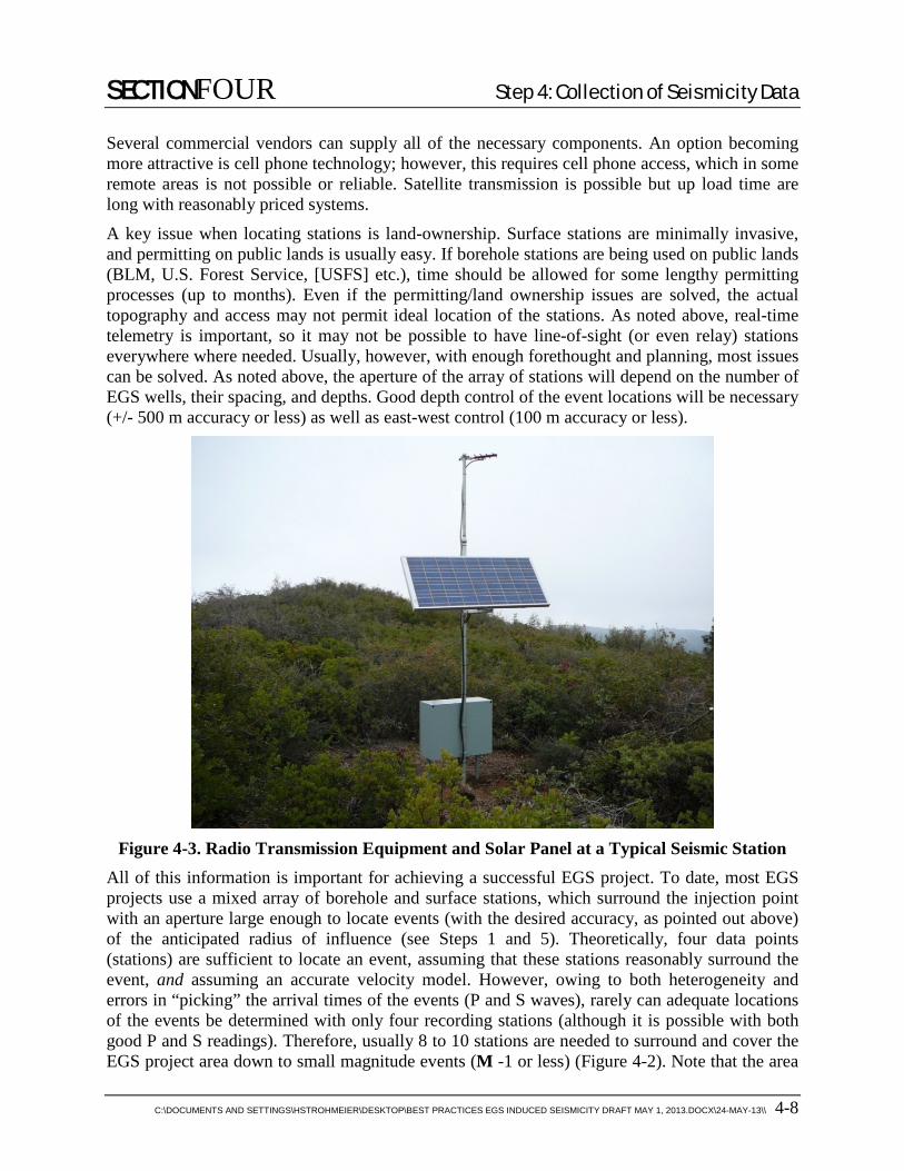
SECTIONFOUR Step 4: Collection of Seismicity Data
C:\DOCUMENTS AND SETTINGS\HSTROHMEIER\DESKTOP\BEST PRACTICES EGS INDUCED SEISMICITY DRAFT MAY 1, 2013.DOCX\24-MAY-13\\ 4-8
Several commercial vendors can supply all of the necessary components. An option becoming more attractive is cell phone technology; however, this requires cell phone access, which in some remote areas is not possible or reliable. Satellite transmission is possible but up load time are long with reasonably priced systems. A key issue when locating stations is land-ownership. Surface stations are minimally invasive, and permitting on public lands is usually easy. If borehole stations are being used on public lands (BLM, U.S. Forest Service, [USFS] etc.), time should be allowed for some lengthy permitting processes (up to months). Even if the permitting/land ownership issues are solved, the actual topography and access may not permit ideal location of the stations. As noted above, real-time telemetry is important, so it may not be possible to have line-of-sight (or even relay) stations everywhere where needed. Usually, however, with enough forethought and planning, most issues can be solved. As noted above, the aperture of the array of stations will depend on the number of EGS wells, their spacing, and depths. Good depth control of the event locations will be necessary (+/- 500 m accuracy or less) as well as east-west control (100 m accuracy or less).
Figure 4-3. Radio Transmission Equipment and Solar Panel at a Typical Seismic Station
All of this information is important for achieving a successful EGS project. To date, most EGS projects use a mixed array of borehole and surface stations, which surround the injection point with an aperture large enough to locate events (with the desired accuracy, as pointed out above) of the anticipated radius of influence (see Steps 1 and 5). Theoretically, four data points (stations) are sufficient to locate an event, assuming that these stations reasonably surround the event, and assuming an accurate velocity model. However, owing to both heterogeneity and errors in “picking” the arrival times of the events (P and S waves), rarely can adequate locations of the events be determined with only four recording stations (although it is possible with both good P and S readings). Therefore, usually 8 to 10 stations are needed to surround and cover the EGS project area down to small magnitude events (M -1 or less) (Figure 4-2). Note that the area

SECTIONFOUR Step 4: Collection of Seismicity Data
C:\DOCUMENTS AND SETTINGS\HSTROHMEIER\DESKTOP\BEST PRACTICES EGS INDUCED SEISMICITY DRAFT MAY 1, 2013.DOCX\24-MAY-13\\ 4-9
of seismicity will grow over time; this must be accounted for in station coverage and layout. Accurate velocity models (3-D) are also needed to correct for wave path effects as well as any temporal changes in velocity structure as the reservoir evolves. Note also that as the EGS operation proceeds, it may be necessary to add and/or move stations to adequately cover the seismicity.
Finally, it is important to calibrate the sensors and array before operation begins. Needed is the polarity of the sensors ( i.e., is up motion on the recorded data up ground motion, is up east on the east-west horizontal, is up on the north-south horizontal north, etc?). Very careful tracing of the signals (from the ground all the way through the system to the final seismogram) is necessary. This can be done with a known source (explosion that records well all first motions at each station), side-by-side comparisons of all stations before deployment, recording a large regional event with known ground motions, etc.). This is necessary for accurate focal mechanisms and moment tensor solutions.
In addition, if possible, calibration shots (deep sources where the location of the shot (preferably at the reservoir level) can be used for first motion detection as well as obtaining velocity models to be used in event locations. Although this sounds simple in theory, local geologic complexity and heterogeneity often complicate data interpretation.
4.3.4 Data Archiving and Processing Requirements Once data collection starts, the usual procedure is to collect the data at a central point and have software in place to detect events of interest. For regulatory compliance, operational understanding, and public communication, real time analysis will be needed.
The order and timing of processing may be different before the main EGS injection begins versus after the injection has begun. In either case, it will be necessary to have initial real-time locations and magnitudes of events posted to a publicly available web site. This can be accomplished with available commercial software that can be customized for any site. A variety of commercial products are in place to do so, but usually the application must be customized for the particular site, depending on the amount and magnitude range of the seismicity. These commercial packages, which are often sold with the microearthquake recording hardware, usually offer such capability as automatic real-time detection of the events (based on user-specified criteria such as number of individual triggers, which are in turn based on signal-to-noise ratio and the frequency content of each signal at each individual station, in a specified time window). Once an event is detected, a pre-specified time window of all channels of data (usually based on size of the detected event) is saved for processing, either in real time with automatic picking, or at a later time by a person who “hand picks” the events. In either case, it is important to save the total waveforms of all channels of data from each event. In most cases, the data are continuously coming into a central collection point. Consequently, it is possible with today’s large memory disks (terabytes of storage are very affordable) to not only store the automatically detected events, but also to store all of the continuous data for later analysis. This would allow going back and sifting through all of the data to see if any events were missed. While such effort may not be necessary if hundreds of events are being detected, it may be worthwhile, especially in some areas of low seismicity, to have all of the continuous data.
Depending on the location of the project and collaborators with public entities, it may be possible to interest such organizations as the USGS and IRIS to archive the data at reasonable costs. A

SECTIONFOUR Step 4: Collection of Seismicity Data
C:\DOCUMENTS AND SETTINGS\HSTROHMEIER\DESKTOP\BEST PRACTICES EGS INDUCED SEISMICITY DRAFT MAY 1, 2013.DOCX\24-MAY-13\\ 4-10
certain amount of processing is also available from these organizations if the data are of high quality.
With good waveform data in hand, there are a variety of options and ways to process the data. The objective in this document is not to give an entire summary of earthquake analysis (books have been written about it [Aki and Richards, 2009], but to point out basic needs and sources of information. (It is assumed that the operators who need to understand the microearthquake data will have access to an experienced seismologist.)
The minimal needs are accurate locations, especially depths, times, magnitude determinations, and some source mechanism information. Location programs are commercially available (using both P and S wave data) that use either 1-D or 3-D models; these are usually least-squared types of solutions and sometimes cubic spline models. The challenge in using 3-D location programs is to derive accurate 3-D velocity models. The usual practice is to use the seismicity to invert for 3-D velocity structure and location together, using tomographic inversion methods (Tomo 3-D is one such program in use). Programs incorporating anisotropy are being developed, but are not available yet; the drawback to these programs, versus location programs such as the USGS Hypoinverse and various versions, is the amount of data required to derive an accurate model with adequate resolution. These programs need many seismic events that are distributed throughout the volume of interest. That is, many ray paths are needed to image the volume in enough detail to derive an accurate velocity model. In tomography, the pixel size is determined by how many ray paths penetrate each pixel. The more ray paths, the smaller the pixels can be. The more complex the geologic structure, the smaller the pixels need to be.
One way to address resolution and precision issues is to use differencing methods with either 1-D or 3-D velocity models i.e., “double difference” methods. This technique cancels out the ray path differences by using events close to one another (common stations for close events), which largely removes the path effects.
The double-difference (DD) earthquake location method was developed to relocate seismic events in the presence of measurement errors and earth model uncertainty. (See http://www.ldeo.columbia.edu/~felixw/DD.html, [Waldhauser, F. and W.L. Ellsworth, 2000], [Waldhauser, F., 2001], [Prejean, St., W.L. Ellsworth, M. Zoback, and F. Waldhauser, 2002].) The method is an iterative least-squares procedure that relates the residual between the observed and predicted phase travel-time difference, for pairs of earthquakes observed at common stations, to changes in the ray path connecting their hypocenters through the change of the travel times for each event with respect to the unknown. When the earthquake location problem is linearized using the double-difference equations, the common mode errors cancel, principally those related to the receiver-side structure. Thus avoided is the need for station corrections or high-accuracy of predicted travel times for the portion of the ray path that lies outside the focal volume. This approach is especially useful in regions with a dense distribution of seismicity, i.e., where distances between neighboring events are only a few kilometers or less. But there must be enough events close together to do this. (USGS uses a combination of both, i.e., Tomo DD.)
Magnitude determination is not straightforward for smaller events. (see http://vulcan.wr.usgs.gov/Glossary/Seismicity/description_earthquakes.html and http://www.seis.utah.edu/EQCENTER/LISTINGS/magsum.htm). One approach is to take the spectra of events and filter to simulate as if the data were recorded on a Wood-Anderson instrument and determine the Richter magnitude, but this is not often done. Sometimes coda

SECTIONFOUR Step 4: Collection of Seismicity Data
C:\DOCUMENTS AND SETTINGS\HSTROHMEIER\DESKTOP\BEST PRACTICES EGS INDUCED SEISMICITY DRAFT MAY 1, 2013.DOCX\24-MAY-13\\ 4-11
magnitudes are used based on empirical data for each region, using larger events and extrapolating to smaller events.
What is more common and more reliable is using moment magnitude (M). However, proper instrumentation is required to capture the low frequency level of the event, which may not be possible if high frequency geophones are used. It is derived by taking the waveform data into the frequency domain and correcting for instrument response, such that the displacement spectra are obtained. From the DC level of the spectra, the moment can be derived and a moment magnitude determined using empirical formulas. One such formula is M = 2/3 log10(Mo) - 10.7 (Hanks and Kanamori, 1979) (Mo = seismic moment in dyne-cm). The moment magnitude relation may also be different for different region and should be calibrated for each area.
Source-mechanism studies are important, but as mentioned before, routine moment tensor calculations are difficult using high-frequency arrays that typically cover only part of the total radiation pattern of an earthquake. In addition, at higher frequencies usually recorded with smaller events, the earth structure has a larger effect on wave paths. Thus, it is more difficult to obtain reliable moment tensor solutions. If moment tensor solutions are desired (they are important for gaining an understanding of the failure mechanisms associated with the reservoir creation process), it will be necessary to set out instrumentation that can record the low-frequency component of the seismic waveforms, as well as having a detailed velocity model of the geology.
4.4 SUMMARY Gathering the correct seismic array data is essential at all stages of the EGS project. This will allow a variety of processing to be done, both in real time and after data have been collected. There are a few reasons for properly collecting seismic data: achieving public acceptance, performing risk assessment, and monitoring/understanding the EGS reservoir. Accurate real time data are necessary for all of those reasons. The detail and amount of data will depend on site conditions and the EGS reservoir characteristics, and the proximity to populated communities and the anticipated risk and hazards.
4.5 SUGGESTED READING Lee, W.H.K. and Stewart, S.W., 1981, Principles and applications of microearthquake networks,
Academic Press, 293 p.

SECTIONFIVEStep 5: Hazard Evaluation of Natural and Induced Seismic Events
C:\DOCUMENTS AND SETTINGS\HSTROHMEIER\DESKTOP\BEST PRACTICES EGS INDUCED SEISMICITY DRAFT MAY 1, 2013.DOCX\24-MAY-13\\ 5-1
5. Section 5 F IVE Step 5: H azard Evaluation of Natu ral and Induced Seismic Events
5.1 PURPOSE The purpose of Step 5 is to estimate the ground shaking hazard at a proposed EGS site due to natural (tectonic) seismicity and induced seismicity. Assessing the ground shaking hazard from natural seismicity will provide a baseline from which to evaluate the additional hazard from induced seismicity. This is a critical step to assessing the probability of exceeding the criteria specified in Step 3.
Hazard is defined as the effect of a physical phenomenon (such as an earthquake or induced seismic event) that will result in an unacceptable consequence (damage, loss, annoyance, etc.). Structural (non-cosmetic) damage can only result when a structure undergoes several cycles of ground shaking. The resulting seismic loading induces strains in the structure resulting in failure of structural components. No cases are known to date where geothermal-induced seismicity has caused structural (non-cosmetic) damage (see definition), because, in general, the seismic events are of small magnitude (< M 4.0). However, because the potential may exist, given some specific circumstances, hazard analyses need to be performed.
An earthquake can present several types of hazards; however, for induced seismic events, we are primarily concerned with ground shaking. Once the ground shaking hazard is quantified, associated secondary hazards such as liquefaction and slope failure (e.g., landsliding) can be evaluated.
Step 5 should be performed before any geothermal stimulations and operations are initiated. Characterization of future induced seismicity at a site is a very complex and difficult problem; thus, assessments must be based on case histories and numerical modeling that incorporates specific site characteristics. The hazard analyses should be updated once data and information on the EGS seismicity become available.
Two approaches can be taken to assess the ground shaking hazard at a proposed site: a probabilistic seismic hazard analysis (PSHA) and a deterministic seismic hazard analysis (DSHA). Hazard results feed into risk analysis as described in Section 6. Probabilistic hazard is more useful for risk analysis because it provides the probabilities of specified levels of ground motions being exceeded. Scenario-based risk analysis using the results of DSHA is useful to describe potential maximum effects to stakeholders.
Several physical factors control the level and character of earthquake ground shaking. These factors are, in general: (1) rupture dimensions, geometry, orientation, rupture type and stress drop of the causative fault; (2) distance from the causative fault; (3) magnitude of the earthquake; (4) the rate of attenuation of the seismic waves along the propagation path from the source to site; and (5) site factors including the effects of near-surface geology, particularly from soils and unconsolidated sediments. Other factors, which vary in their significance depending on specific conditions, include slip distribution along the fault, rupture directivity, footwall/hanging-wall effects, and the effects of crustal structure such as basin effects.
The ground motion hazard should be expressed in terms of peak ground acceleration (PGA), acceleration response spectra (to compare with spectra from natural earthquakes and building code design spectra), peak ground velocity (PGV), and velocity spectra. PGV (or PPV) will be needed for comparison with cosmetic and structural building damage criteria, with criteria for vibration sensitive research and manufacturing facilities, and for human activity interference.

SECTIONFIVEStep 5: Hazard Evaluation of Natural and Induced Seismic Events
C:\DOCUMENTS AND SETTINGS\HSTROHMEIER\DESKTOP\BEST PRACTICES EGS INDUCED SEISMICITY DRAFT MAY 1, 2013.DOCX\24-MAY-13\\ 5-2
5.2 OVERVIEW OF APPROACH PSHAs should be performed first for the natural seismicity, and then for the EGS-induced seismicity (an addition to the natural hazard). As discussed in Section 1, the hazard from natural seismicity for sites in the U.S. can be obtained from the USGS National Seismic Hazard Maps. However, the hazard estimates from the USGS maps are not site-specific. Because a comparison of the hazard from natural and induced seismicity is required, site-specific analyses are needed at this stage. The PSHA methodology and each step in the hazard evaluation process are described in detail in the next sections. DSHAs can be performed for additional insight into the seismic hazard.
5.2.1 Estimate the Baseline Hazard from Natural Seismicity The major steps to be performed to evaluate the baseline hazard from natural seismicity are:
1. Evaluate the historical seismicity in the site region and calculate the frequency of occurrence of background seismicity based on the earthquake catalog. If baseline seismic monitoring was performed in the EGS geothermal project area, that data should be incorporated into the earthquake catalog.
2. Characterize any active or potentially active faults in the site region and estimate their source parameters (source geometry and orientation, rupture process, maximum magnitude, recurrence model, and rate) for input into the hazard analysis.
3. For communities that may be impacted by future EGS-induced seismicity, evaluate the geological site conditions beneath the communities and, if practical, estimate the shear-wave velocities of the shallow subsurface.
4. Select appropriate ground motion prediction models for tectonic earthquakes for input into the hazard analysis.
5. Perform a PSHA and produce hazard curves and hazard maps if required, to assess the baseline hazard due to natural seismicity before any induced seismicity occurs.
5.2.2 Estimate the Hazard from Induced Seismicity For comparison to natural seismicity, estimating the hazard from EGS-induced seismicity particularly before EGS operations are initiated, is more difficult. The database of induced seismicity observations in terms of both seismic source characterization and ground motion prediction, is also much smaller than for natural seismicity. However, as more information becomes available (particularly seismic monitoring results), the hazard can be updated and the uncertainties in the hazard results reduced. Possible steps that should be taken include:
1. Evaluate and characterize the tectonic stress field based on focal mechanisms of natural earthquakes, the geologic framework of the potential geothermal area and any other available data, particularly the results from any prior seismic monitoring.
2. Review known cases of induced seismicity and compare the tectonic and geologic framework from those cases with the potential EGS area.
3. Evaluate the characteristics and distribution of pre-existing faults and fractures. This characterization will be useful in assessing the potential and characteristics of future EGS-induced seismicity as related to the tectonic stress field.

SECTIONFIVEStep 5: Hazard Evaluation of Natural and Induced Seismic Events
C:\DOCUMENTS AND SETTINGS\HSTROHMEIER\DESKTOP\BEST PRACTICES EGS INDUCED SEISMICITY DRAFT MAY 1, 2013.DOCX\24-MAY-13\\ 5-3
4. Review and evaluate available models for induced seismicity that estimate the maximum magnitude of induced seismicity based on injection parameters.
5. Review and select empirical ground motion prediction model(s) appropriate for induced seismicity, if any are available, or at a minimum, one that is appropriate for small to moderate magnitude natural earthquakes (moment magnitude [M] < 5.0).
6. Perform a PSHA and produce hazard curves and hazard maps if required, to assess the EGS-induced seismicity hazard.
7. An optional step is to calculate scenario ground motions from the maximum induced seismic event by performing a DSHA.
5.3 PSHA METHODOLOGY AND COMPUTER PROGRAMS The objectives in a PSHA are to evaluate and characterize potential seismic sources, the likelihood of earthquakes of various magnitudes occurring on or within those sources, and the likelihood of the earthquakes producing ground motions over a specified level (Figure 5-1). The PSHA methodology allows for the explicit inclusion of the range of possible interpretations in components of the seismic hazard model, including seismic source characterization and ground motion estimation. Uncertainties in models and parameters can be incorporated into the PSHA through the use of logic trees.
The PSHA methodology is based on the model developed principally by Cornell (1968). The occurrence of earthquakes on a fault is assumed to be a Poisson process. The Poisson model is widely used and is a reasonable assumption in regions where data are sufficient to provide only an estimate of average recurrence rate (Cornell, 1968). The occurrence of ground motions at the site in excess of a specified level is also a Poisson process, if (1) the occurrence of earthquakes is a Poisson process, and (2) the probability that any one event will result in ground motions at the site in excess of a specified level is independent of the occurrence of other events.
There are publically available computer programs that can be used to perform a PSHA. We recommend the two most available programs that have been validated in the Pacific Earthquake Engineering Research (PEER) Center-sponsored Validation of PSHA Computer Programs Project (Thomas et al., 2010). They include the HAZ program developed by Norm Abrahamson, which is available from the author upon request, and EZ-FRISK, which can be obtained through license from Risk Engineering Inc.
The following describes in more detail the steps to perform a PSHA for natural seismicity outlined in Section 6.2.1.
5.3.1 Evaluate Historical Seismicity In Step 4, a historical earthquake catalog is compiled. The value of evaluating the historical seismicity of the site region is two-fold: (1) it can be used to characterize the natural seismicity, and (2) it can provide some insight into the potential for induced seismicity. Note there certainly are exceptions, the most important being that induced seismicity can occur in regions with low historical seismicity.

SECTIONFIVEStep 5: Hazard Evaluation of Natural and Induced Seismic Events
C:\DOCUMENTS AND SETTINGS\HSTROHMEIER\DESKTOP\BEST PRACTICES EGS INDUCED SEISMICITY DRAFT MAY 1, 2013.DOCX\24-MAY-13\\ 5-4
Figure 5-1. The Steps in Performing a PSHA

SECTIONFIVEStep 5: Hazard Evaluation of Natural and Induced Seismic Events
C:\DOCUMENTS AND SETTINGS\HSTROHMEIER\DESKTOP\BEST PRACTICES EGS INDUCED SEISMICITY DRAFT MAY 1, 2013.DOCX\24-MAY-13\\ 5-5
5.3.2 Characterize Seismic Sources Seismic source characterization is concerned with three fundamental elements: (1) the identification, location, and geometry of significant sources of earthquakes; (2) the maximum sizes of the earthquakes associated with these sources; and (3) the rate at which the earthquakes occur.
Two types of earthquake sources are typically characterized in PSHAs: (1) fault sources; and (2) areal source zones. Fault sources are modeled as three-dimensional fault surfaces, and details of their behavior are incorporated into the source characterization. Areal source zones are regions where earthquakes are assumed to occur randomly.
Uncertainties in the seismic source parameters can be incorporated into PSHA using a logic tree approach. In this procedure, values of the source parameters are represented by the branches of logic trees with weights that define the distribution of values. A sample logic tree is shown in Figure 5-2.
Figure 5-2. Seismic Hazard Model Logic Tree
In a PSHA, earthquakes of a certain magnitude are assumed to occur randomly along the length of a given fault or segment (Figure 5-1). The distance from an earthquake to the site is dependent on the source geometry, the size and shape of the rupture on the fault plane, and the likelihood of the earthquake occurring at different points along the fault length. The distance to the fault is

SECTIONFIVEStep 5: Hazard Evaluation of Natural and Induced Seismic Events
C:\DOCUMENTS AND SETTINGS\HSTROHMEIER\DESKTOP\BEST PRACTICES EGS INDUCED SEISMICITY DRAFT MAY 1, 2013.DOCX\24-MAY-13\\ 5-6
defined to be consistent with the specific ground motion prediction model used to calculate the ground motions. The distance, therefore, is dependent on both the dip and depth of the fault plane, and a separate distance function is calculated for each geometry and each ground motion prediction model. The size and shape of the rupture on the fault plane are dependent on the magnitude of the earthquake; larger events rupture over longer and wider portions of the fault plane. Rupture dimensions are modeled following standard magnitude-rupture area and rupture-width relationships.
5.3.2.1 Fault Geometry
The first step in characterizing potential seismic sources is to identify which known faults are “active” and hence, seisenic seismogenic, i.e., capable of producing earthquakes in the future. The criteria for defining an active fault varies widely among U.S. government regulatory agencies. For example, in California, a fault that has moved in the past 35,000 years is considered an “active” fault. A “conditionally active” fault is defined as a fault that has ruptured in Quaternary time (past 1.6 million years) but its displacement history is unknown in the past 35,000 years. The USGS maintains the Quaternary Fault and Fold Database that can be used to identify active faults during the Quaternary and included in the site-specific PSHA. The database also contains many of the parameters such as fault location, strike, and dip that are needed, although parameter uncertainties may not be included.
For each active fault to be included in the hazard analysis, the location and orientation (strike, dip, and dip direction), segmentation model, thickness of the seismogenic zone, style of faulting (strike-slip, normal, or reverse/thrust) are needed (Figure 5-3). This information can generally be adopted from the USGS database. The top and bottom of each fault are also required. If the fault is expressed at the surface, the top is zero. For buried faults, an estimate must be made unless subsurface information is available such as seismic data. The bottom of the fault can be estimated from the seismicity data, which will delineate the bottom of the seismogenic crust, usually 12 to 20 km in the western U.S. If the fault is long, greater than 60 to 80 km, the fault may be segmented. That is, portions of the fault, rather than the whole fault, may rupture. If such information exists from paleoseismic and/or historical data, the rupture segmentation model needs to be included in the PSHA.
5.3.2.2 Maximum Magnitude
The maximum earthquake that a fault or fault segment can generate is usually derived by the use of empirical relationships between magnitude and either rupture length or rupture area (rupture length times rupture width), unless the maximum earthquake has been observed historically. There are other approaches, but the use of rupture dimensions is most common. The most commonly used set of empirical relationships are by Wells and Coppersmith (1994). For example, based on rupture length, a 40 km-long fault can generate a M 6.9 earthquake based on Wells and Coppersmith (1994). The USGS Fault and Fold Database also provides values of maximum magnitude, although uncertainties are not included.

SECTIONFIVEStep 5: Hazard Evaluation of Natural and Induced Seismic Events
C:\DOCUMENTS AND SETTINGS\HSTROHMEIER\DESKTOP\BEST PRACTICES EGS INDUCED SEISMICITY DRAFT MAY 1, 2013.DOCX\24-MAY-13\\ 5-7
Source: Brumbaugh, 1999
Figure 5-3. The three principal types of faults (a) strike-slip faults, (b) reverse faults, and (c) normal faults.
5.3.2.3 Recurrence Parameters
The recurrence parameters include recurrence model, recurrence rate (slip rate or average recurrence interval for the maximum event), slope of the recurrence curve (b-value), and maximum magnitude. The recurrence relationships for the faults are modeled using the truncated exponential, characteristic earthquake, and the maximum magnitude recurrence models (Figure 5-2). These models are generally weighted in a PSHA to represent one’s judgment on their applicability to the sources. For the areal source zones, only an exponential recurrence relationship is assumed to be appropriate.

SECTIONFIVEStep 5: Hazard Evaluation of Natural and Induced Seismic Events
C:\DOCUMENTS AND SETTINGS\HSTROHMEIER\DESKTOP\BEST PRACTICES EGS INDUCED SEISMICITY DRAFT MAY 1, 2013.DOCX\24-MAY-13\\ 5-8
The truncated exponential model is a form of the classical Gutenbeg-Richter model. The model where faults rupture with a “characteristic” magnitude on specific segments is described by Schwartz and Coppersmith (1984). The characteristic model, often used in PSHAs, is the numerical model of Youngs and Coppersmith (1985).
The maximum magnitude (or moment) model can be regarded as an extreme version of the characteristic model (Wesnousky, 1986). In the maximum magnitude model, there is no exponential portion of the recurrence curve, i.e., events are modeled with a normal distribution about the characteristic magnitude.
The average recurrence interval for the characteristic or maximum magnitude event defines the high magnitude (low likelihood) end of the recurrence curve. When combined with the relative frequency of different magnitude events from the recurrence model, the recurrence curve is established.
5.3.2.4 Recurrence Rates
The recurrence rates for the fault sources are defined either by the slip rate, or by the average recurrence interval for the maximum or characteristic event and the recurrence b-value. An example of recurrence intervals, sometimes referred to as inter-event times, would be the approximately 300-year interval of the North Coast segment of the San Andreas fault, which ruptured in the Great 1906 M 7.8 San Francisco, California earthquake. Slip rate is defined as fault displacement divided by the time period in which displacement occurred. Slip rate is a proxy for activity rate. Recurrence interval is the time period between individual earthquakes. (The North Coast segment of the San Andreas fault has a slip rate of about 20 mm/yr.)
5.3.3 Areal Sources Areal sources are usually used to account for “background” earthquakes. The hazard from background (floating or random) earthquakes that are not associated with known or mapped faults must be incorporated into the hazard analysis. In most of the western U.S., the maximum magnitude for earthquakes not associated with known faults usually ranges from M 6 to 7. Repeated events larger than these magnitudes probably produce recognizable fault-or fold-related features at the earth’s surface. For areal source zones, only the areas, maximum magnitude, and recurrence parameters (based on the historical earthquake record) need to be defined.
5.3.4 Characterize Site Conditions The geologic conditions beneath a site can significantly influence the level and nature of ground shaking. In very general terms, soil sites will have a higher level of ground motions than rock sites due to site amplification. Hence, to be able to predict the ground shaking at a site, particularly a soil site, the underlying shear-wave velocity (VS) structure is needed to a depth of at least 30 m and deeper if possible. The parameter VS30 (the average VS in the top 30 m) is used in ground motion prediction models and in the U.S. building code (called the International Building Code or IBC) to classify different site conditions. For example, the NEHRP site classification has six site classes: hard rock, rock, very dense soil and soft rock, stiff soil, soft soil, and soft liquefiable soil. The VS profile (VS versus depth) is often used in ground motion prediction models to quantify site and building foundation responses. The VS profile at a site can

SECTIONFIVEStep 5: Hazard Evaluation of Natural and Induced Seismic Events
C:\DOCUMENTS AND SETTINGS\HSTROHMEIER\DESKTOP\BEST PRACTICES EGS INDUCED SEISMICITY DRAFT MAY 1, 2013.DOCX\24-MAY-13\\ 5-9
be obtained through geophysical surveys such as downhole and crosshole surveys, surface wave techniques, and microtremor surveys.
5.3.5 Select Ground Motion Prediction Models To characterize the ground motions at a specified site as a result of the seismic sources considered in the PSHA and DSHA, ground motion prediction models for spectral accelerations are used. These models are generally based on strong motion data and relate a specified ground motion parameter (e.g., PGA) with the magnitude and distance of the causative event, and the specific site conditions at the potentially affected site(s). Examples of ground motion prediction models are the recently developed Next Generation of Attenuation (NGA) models developed by the Pacific Earthquake Engineering Research Center (Figure 5-4). These models are appropriate for earthquakes of M 5.0 and greater. A model by Chiou and Youngs (2010) was developed for earthquakes of M 3.0 to 5.5.
The uncertainty in ground motion models is included in the PSHA by using the log-normal distribution about the median values as defined by the standard error associated with each ground motion prediction model.
Source: Abrahamson et al., 2008
Figure 5-4. Comparison of Distance Scaling of PGA for Strike-Slip Earthquakes for VS30 760 m/sec
5.3.6 PSHA Products The primary products of a PSHA are hazard curves that show the annual frequency of exceedance for some specified ground motion parameter (e.g., PGA; Figure 5-5). Often the term “return period,” which is the inverse of the annual frequency of exceedance, is used., The IBC uses an annual frequency of exceedance of 1 in 2,475 or a return period of 2,475 years. The

SECTIONFIVEStep 5: Hazard Evaluation of Natural and Induced Seismic Events
C:\DOCUMENTS AND SETTINGS\HSTROHMEIER\DESKTOP\BEST PRACTICES EGS INDUCED SEISMICITY DRAFT MAY 1, 2013.DOCX\24-MAY-13\\ 5-10
results of a PSHA can also be deaggregated to evaluate what seismic sources are contributing most of the hazard at a site.
Figure 5-5. Seismic Hazard Curves for Peak Horizontal Acceleration
5.4 ADDITIONAL STEPS IN CHARACTERIZING EGS FOR PSHA In typical PSHAs for engineering design, the minimum magnitude considered is M 5.0 because empirical data suggests that smaller events seldom cause structural damage (Bommer et al., 2006). Since no EGS-induced earthquake has exceeded M 5.0 in size to date, the hazard analyses should be performed at lower minimum magnitudes. We suggest that PSHAs be performed for M 4.0 so that the hazard with EGS seismicity can be compared with the baseline hazard from tectonic earthquakes. To provide input into the risk analysis (Step 6), an even lower minimum magnitude may be considered for nuisance effects or interference with sensitive activities.

SECTIONFIVEStep 5: Hazard Evaluation of Natural and Induced Seismic Events
C:\DOCUMENTS AND SETTINGS\HSTROHMEIER\DESKTOP\BEST PRACTICES EGS INDUCED SEISMICITY DRAFT MAY 1, 2013.DOCX\24-MAY-13\\ 5-11
5.4.1 Characterize Local and Regional Stress Field Most induced seismic events will occur on pre-existing zones of weakness, e.g., faults and fractures that are favorably oriented to the tectonic stress field. Knowledge of the local and regional stress field can thus help identify a priori, which features are more likely to be the sources of induced seismicity. The characterization of the stress field can be obtained from in situ stress measurements (e.g., hydraulic fracturing, borehole breakouts, and core-induced fractures). The orientations and magnitudes of the maximum, intermediate, and minimum principal stresses are required. A combination of image log analysis and a diagnostic hydraulic fracturing (extended leak-off test or “minifrac”) is the best approach for measuring in situ stresses. With knowledge of the in situ stress field, a Mohr-Coulomb stress analysis can be performed to assess the critical stress required to trigger slip on favorably-oriented faults that are critically stressed and near failure.
Earthquake focal mechanisms can provide information on the principal stresses but not their absolute magnitudes. Stress fields can be categorized by which style of faulting will be dominant: strike-slip, normal (extensional), and reverse/thrust (compressional) (Figure 5-2).
5.4.2 Develop 3D Geologic Model To the extent practicable and given the available data, a 3D structural and stratigraphic model of the EGS area should be developed that includes pre-existing faults and fractures that could be sources of future induced seismicity. Characterizing any significant favorably oriented fault is critical for assessing the maximum earthquake that could occur (see below). Often 2-D and 3-D models are developed to evaluate the EGS potential of an area in the early stages of a project. This should include evaluations of drilling results, wellbore image logs, seismic reflection data, and any other subsurface imaging data that may exist (e.g., seismic tomography, potential field data, etc.).
5.4.3 Review of Relevant EGS Case Histories In particular, the information on the maximum magnitude and the frequencies of occurrence of case histories of induced seismicity should be reviewed. Numerous publications are available that describe cases of EGS and geothermal-induced seismicity. Majer et al. (2007) summarizes some of the most significant case histories. Geothermal-induced seismicity has occurred in several countries including most notably the U.S., Japan, Australia, France, and Switzerland.
5.4.4 Develop Induced Seismicity Model Developing a model for induced seismicity is the most challenging task in assessing the hazard. Induced seismicity is the interaction between the injection parameters such as injection rates, pressures, and volume and depth of injection, and the in situ lithologic, structural, hydrologic, and thermal conditions (e.g., faults, fractures, rock strength, porosity, permeability, etc.). These are the most challenging geologic characteristics to evaluate because of the difficulty in imaging and the general heterogeneity and complexity inherent in rock masses. Given this challenge, conservative assumptions on the maximum induced event and rates of induced seismicity can be made for upper-bound estimates of the hazard. Best estimates of the hazard can be improved by incorporating the possible ranges of parameters and their uncertainties. In some circumstances, an evaluation of the potential for far-field triggering of a damaging earthquake on a nearby fault

SECTIONFIVEStep 5: Hazard Evaluation of Natural and Induced Seismic Events
C:\DOCUMENTS AND SETTINGS\HSTROHMEIER\DESKTOP\BEST PRACTICES EGS INDUCED SEISMICITY DRAFT MAY 1, 2013.DOCX\24-MAY-13\\ 5-12
due to fluid-injection induced seismicity may be required, although no such cases have been observed to date.
Maximum magnitudes and earthquake rates are the two most important inputs into seismic hazard analyses. The magnitude of an earthquake is proportional to the area of the fault that slips in an event and the amount of that slip. Several conditions must be met for a large and potentially damaging earthquake to occur. There must be a large enough fault, stresses must be high enough to cause slip, and the fault needs to be pre-stressed and near failure.
Predicting the maximum magnitudes of earthquakes due to EGS activities has been a difficult challenge. As recognized by many, the characteristics of induced seismicity are controlled by the nature and distribution of pre-existing fractures and faults, the local stress field in the volume of rock surrounding the well where fluid is being introduced (e.g., Majer et al., 2007), and the characteristics of the pore pressure field due to injection. Empirical relationships have been developed that estimate the magnitude of an earthquake from rupture length, rupture area, and maximum and average event displacement. The best approach to estimating the potential maximum induced earthquake is to characterize the maximum dimensions of pre-existing faults that could rupture in an induced earthquake. To be able to estimate fault dimensions, imaging faults in the subsurface is required.
A number of theoretical approaches have been developed to predict maximum magnitude. All the approaches above depend on an a priori knowledge of the rupture characteristics of future induced seismicity, which requires subsurface characterization of the affected volume of rock around the well. McGarr (1976) relates the sums of the seismic moment released in earthquakes to a change in volume. In the case of fluid injection, this change is the volume added to the system by injection. A second approach is to relate the seismic moment or maximum magnitude to the maximum length or area of pre-existing faults in the volume of rock that will be affected by fluid injection.
A third approach has been proposed by Shapiro et al. (2010) using the parameter “seismogenic index.” Shapiro et al. (2007) observed that under “general conditions,” the number of fluid-induced earthquakes with a magnitude larger than a given value increases approximately proportionally to the injected fluid volume. The seismogenic index depends on the local maximum critical pressure for shear fracturing, the volume concentration of pre-existing fractures, and the poroelastic uniaxial storage coefficient (Shapiro et al., 2010). Along with the injection parameters, the seismogenic index can be used to estimate the probability of a given number of such events during an injection period. Shapiro et al. (2010) applied this technique for six case studies of injection induced seismicity including Cooper Basin, Basel, and Ogachi.
Estimating the rate of EGS seismicity a priori is a significant challenge because the problem is very site-specific and not all factors that can impact rate are quantifiable at this time. However, efforts are underway in the U.S. and Europe where induced seismicity is an important issue (e.g., Basel) to develop probabilistic approaches to estimating ground motions in near-real time for alarm systems. A traffic-light alarm system, which is based on public response, magnitude, and PGV has been used in experiments such as Basel (Section 7). For example, Bachmann et al. (2011) are developing a forecast model by modeling the Basel sequence and testing various statistical models such as the aftershock model for California earthquakes. The intent is to translate the forecast model to probabilistic hazard, e.g., probability for exceeding a ground motion level.

SECTIONFIVEStep 5: Hazard Evaluation of Natural and Induced Seismic Events
C:\DOCUMENTS AND SETTINGS\HSTROHMEIER\DESKTOP\BEST PRACTICES EGS INDUCED SEISMICITY DRAFT MAY 1, 2013.DOCX\24-MAY-13\\ 5-13
5.4.5 Select Ground Motion Prediction Models for Induced Seismicity Almost all existing ground motion prediction models have been developed for M 5.0 and above natural earthquakes, and it has been suggested that there is a break in scaling between small and large earthquakes (Chiou et al., 2010). To our knowledge, no ground motion prediction model for EGS seismicity or geothermal-induced seismicity has been developed and made publically available. In lieu of a model for induced seismicity, the model proposed by Chiou et al. (2010) for small to moderate natural earthquakes (M 3 to 5.5) in California is the next best alternative. Ground motion models for earthquakes smaller than M 5 are being developed by PEER and should be available in 2013. Since the maximum induced earthquake will likely be smaller than M 5.0, the ground motion prediction model only needs to be accurate at short distances (less than 20 km.
5.4.6 Products The products of a PSHA are the same as described in Section 5.3.6 the only difference being is the results will now include potential induced seismicity in addition to background tectonic seismicity.
5.5 SUMMARY The hazard results from the natural and induced earthquakes should be compared to assess the potential increase in hazard associated with the EGS project. The hazard results are fed into Step 6, the risk analysis. The hazard estimates should be updated as new information becomes available after injection activities have commenced, and, if and when, induced seismicity has been initiated. In particular, the results of the seismic monitoring should be evaluated and incorporated into the hazard analyses where possible.
5.6 SUGGESTED READING McGuire, R.K., 2004, Seismic hazard and risk analysis: Earthquake Engineering Research
Institute MNO-10, 221 p.
Reiter, L., 1990, Earthquake hazard analysis, issues and insights: Columbia University Press, New York, 254 p.
Yeats, R.S., Sieh, K., and Allen, C.R., 1997, The geology of earthquakes: Oxford University Press, 568 p.

SECTIONSIX Step 6: Risk Informed Decision Analysis and Tools for Design and Operation of EGS
C:\DOCUMENTS AND SETTINGS\HSTROHMEIER\DESKTOP\BEST PRACTICES EGS INDUCED SEISMICITY DRAFT MAY 1, 2013.DOCX\24-MAY-13\\ 6-1
6. Section 6 SIX Step 6: Risk Info rmed D ecision Analysis and Tools for Design and Operation of EGS
6.1 PURPOSE The purpose of this step is to give guidance for performing a risk analysis whose results will help make decisions with the intent of minimizing the risk of damage, annoyance, or losses that the design and operation of an EGS project might produce, and possibly to maximize the benefits to the operators and to local communities. The detailed risk analysis needs to be time-dependent, because the stress conditions in the EGS field will change in relation to the injection schedule. The risk profile will change accordingly, and finally return to the natural seismicity risk after all the stress perturbations caused by the EGS operation, in and around the EGS field, have dissipated, which could take several decades after stopping injection.
6.2 OVERVIEW OF BEST PRACTICE APPROACH Formal seismic risk analysis started in the mid 20th century to analyze the design of complex systems, and in the 1970s, it developed considerably in its application to the nuclear industry. It is now a mature field that is routinely used with geographic information systems, to analyze projects at the community, state, or regional level. Seismic risk analysis is a well-accepted approach, and its methods and tools are extensively used by local and regional governments and by the insurance industry to predict possible losses from natural catastrophes and to help decide on such things as premiums, fees, and compensation.
6.2.1 Hazard, Vulnerability and Exposure Seismic risk is usually expressed as a probability of all the relevant adverse impacts of the ground shaking occurring. For EGS projects, we are concerned with the impact of the seismicity induced by the EGS operation, which if it does not have all the attributes of the standard type of analysis performed for natural catastrophes, still possesses some of its most important elements. Some of the effects of the seismic ground shaking are in the form of “physical” consequences, such as structural damage to houses and other engineered structures, or to the physical environment. There is also “non-physical” damage to humans, physiological and psychological in nature. For example people’s sleep can be disturbed, or they can develop anxieties from the frequent occurrence of small earthquakes that are otherwise physically non-damaging. Much of this anxiety is caused by concern over property and homes, even if the ground motion is insufficient to cause structural or cosmetic damage.
As described in Section 5, the seismic hazard that is of importance here is the ground shaking that is produced at a location by the occurrence of an earthquake, and seismic hazard analysis describes the potential for this ground shaking. It is expressed by a probability distribution of the selected ground shaking parameter (e.g., PGA, PGV, and/or response spectra).
Vulnerability describes how the component of a system can fail or lose its function. For a building or an engineered facility, it describes probabilistically the state or level of damage that it will be in after being subjected to a seismic ground shaking (e.g., four possible states of damage: V-L, L, M, and H). It is expressed as a probability of being in a given state of damage for a given level of ground shaking.

SECTIONSIX Step 6: Risk Informed Decision Analysis and Tools for Design and Operation of EGS
C:\DOCUMENTS AND SETTINGS\HSTROHMEIER\DESKTOP\BEST PRACTICES EGS INDUCED SEISMICITY DRAFT MAY 1, 2013.DOCX\24-MAY-13\\ 6-2
Exposure is typically the cost of repair for a given building. For non-physical damage such as annoyance, loss of life, or way-of-life disturbances, there is no agreed-upon associated monetary cost measure, and it is more appropriate to predict how populations are affected, in terms of the number of lives lost, or the number of people potentially inconvenienced or whose way of life would be potentially disturbed by the ground shaking. Loss is a monetary expression of the damage caused to items exposed, such as cost of re-painting room interiors, broken windows, structural repairs, and so on.
6.2.2 General Framework of a Best-Practice Risk Analysis for EGS The elements at risk comprise essentially all the items of the living environment affected by ground shaking in the vicinity of the EGS field. This includes residential and commercial buildings, industrial facilities, business offices, infrastructures, etc., and people, animals, and the environment. In some cases where damage to components (buildings, etc.) in the study area can affect others outside of the area, this must be included in the study, such as in the case of business interruptions. A simple example would be the failure of a bridge that is the only access to a remote community. The community’s inhabitants may not suffer any damage, physical or annoyance, but their way-of-life may be drastically affected by the failure of the bridge. Businesses in the community might lose business opportunities. More common during small earthquakes is the loss of power due to damage to power poles.
For the case of physical damage, the first parameter of interest is the monetary value of the losses caused by the ground shaking. As important as the monetary loss, is a measure of the level of annoyance for non-physical damage. Loss of life should also be considered, but it has been found to be a negligible risk in previous studies (SERIANEX, 2009), especially if it can be demonstrated that the maximum magnitudes of EGS-induced earthquake are small (i.e., M < 4).
The general framework to estimate a useful figure of merit is summarized by the risk equation:
Risk = Hazard • Vulnerability • Cost of consequences Eq. (6-1)
The elements at risk (buildings, etc.) in the area of study constitute the “system” to be analyzed. An earthquake will damage part of the system, the final result being uncertain due to the uncertain behavior of each of the components in the system. For a given magnitude earthquake there could be many possible final states of the system, depending on which buildings are damaged and how much damage they suffered.
In the above expression,
• The Hazard is characterized in probability terms, by a hazard curve that describes the probability distribution of the future ground shaking.
• Vulnerability is also characterized probabilistically by a representation of the uncertain behavior of the element considered at risk (e.g. a structure). Even if the amplitude of the ground shaking were perfectly known, the damage outcome would be uncertain, and would be described by vulnerability curves that give the probability of damage outcome levels as a function of the amplitude of the ground shaking.

SECTIONSIX Step 6: Risk Informed Decision Analysis and Tools for Design and Operation of EGS
C:\DOCUMENTS AND SETTINGS\HSTROHMEIER\DESKTOP\BEST PRACTICES EGS INDUCED SEISMICITY DRAFT MAY 1, 2013.DOCX\24-MAY-13\\ 6-3
• Cost of Consequences: For physical damage, the cost of consequences is what it will cost to replace or repair a damaged building, or to repair it. Strictly, the cost of repair or replacement should also be treated as an uncertain parameter, but in practice, it is relatively better known than the other parameters (hazard, and vulnerability), and consequently it is often quantified deterministically, as the value of repair for a particular level of damage. In the case of non-physical damage, it would be difficult to assign a monetary value on damage such as annoyance and it is suggested to estimate a level of annoyance and the number of persons annoyed.
Eq. 6.1 represents the risk (or the monetary loss) of the total effect of all possible expected ground shaking that will be experienced, combined with all possible damage outcomes, with their respective cost.
Mathematically, it is a double integration (summation) first over all ground shaking values weighted by their probability densities (from the hazard), and second over damage levels weighted by the probability density of achieving the various levels of damage, and multiplied by the cost of repair for each possible outcome.
In a standard risk analysis, the first step consists of identifying all the possible outcomes or end-states of the system after an earthquake. A number of different techniques are available to model the behavior of the system and identify the possible end-states. The fault tree analysis method (USNRC, 1981) is often used for this purpose. However this method needs to consider every possible combination of different failure states for each of the components in the system. For EGS which is concerned with areas with possibly many impacted buildings (the components of the system), this would lead to a quasi-infinite set of combinations (for example, if there are 2 buildings, each with 4 possible damage states [V-L, L, M, and High], the number of combinations is 16. For n buildings each with 4 possible damage states, the number is 4n). This could not be handled with present computational power. Instead, the risk is estimated for aggregation of small sub-areas (such as zip code areas), and for classes of structures (wood residential structures, 1 story, 2 stories, concrete structures, steel structures, etc., see HAZUS, 2010, for examples). Then the risks are added for the entire study region. The sub-areas are generally considered to be statistically independent, to allow simple summation of the numerical value of the risk, but some methods account for spatial correlation.
Notable differences exist in the nature of the hazard and the range of possible consequences between standard application cases (i.e., natural seismicity) and EGS that require choice of customized methods for which no dominant method exists yet. The main differences are in the range of earthquake magnitudes, and consequently, the range of damage to consider. SRA applications in the last few decades considered earthquakes with magnitudes greater than M 4.5 or 5. They were mostly concerned with dominant earthquakes in the range of magnitudes M 5.5 to 7.5 that could potentially damage well-engineered civil engineering facilities such as dams, bridges, nuclear power plants, etc. They also considered all large earthquakes within several hundreds of kilometers, typically 250 to 300 km, and for earthquakes at depths of 5 to 20 km, which are the dominant contributors to risk in critical facilities. Consequently, the models used in the characterization of the seismic hazard were calibrated for these ranges of magnitudes and distances, and do not represent well the very small magnitude and shallow earthquakes of induced seismicity, and the very short distances and small depths.

SECTIONSIX Step 6: Risk Informed Decision Analysis and Tools for Design and Operation of EGS
C:\DOCUMENTS AND SETTINGS\HSTROHMEIER\DESKTOP\BEST PRACTICES EGS INDUCED SEISMICITY DRAFT MAY 1, 2013.DOCX\24-MAY-13\\ 6-4
Recent seismic risk studies for EGS and other similar projects have started developing more appropriate models (SERIANEX, 2009), but they are region-dependent and every new EGS study will need its own set of customized models. A similar situation exists for the characterization of vulnerabilities. Most existing models were developed for natural catastrophes for which damage is often substantial, with building collapses, losses of life, infrastructure demolished, etc., and little interest in annoyance. In contrast, EGS damage, if any, is generally concentrated in the range of small damage, primarily cosmetic and annoyance may be an important part of the consequences.
6.3 SEISMIC HAZARD CHARACTERIZATION FOR RISK ASSESSMENT
6.3.1 Probabilistic and Scenario Hazard It is customary to base the design of expensive or critical facilities on expected risk estimates to compare the various alternative designs and operational options to select the most appropriate one that will minimize the long-term risk, and satisfy a variety of other, not necessarily technical or financial criteria. This requires a probabilistic estimate of the seismic hazard. However it is also necessary to provide information on ”What would happen in the reasonably worst case?”, if only to check that general safety is preserved, but also, largely to communicate and reassure the potentially affected population. Therefore a scenario earthquake must be constructed that will reflect reasonably and accurately such possibility. This will include selecting a magnitude and a location of the earthquake from which a ground shaking mean value and probability distribution will be estimated for each point of interest in the affected area.
6.3.2 Size of the Assessment Area Performing a seismic risk assessment requires knowledge of the level of ground shaking at the location of each item at risk (buildings, etc.). For a probabilistic risk estimate a hazard curve for a single parameter is needed (i.e., PGA or PGV). For a scenario estimate, the hazard curve is replaced by a probability distribution of the ground shaking parameter for the selected scenario earthquake. The hazard curve is also provided in the form of a probability of exceedance curve and is used in the same fashion as the hazard curve of the probabilistic case, but it is not necessarily associated with any annual probability of occurrence (i.e., how frequently it occurs).
In both cases (probabilistic and scenario analysis) the ground-shaking predictions must be done for each location in the entire area potentially affected by the induced seismicity of the EGS field. This area of risk assessment is of radius R, centered on the injection well(s). The size of R (km) depends on the local geological environment, on the size of the EGS field, and on the injection parameters, but the deciding parameter is the distance at which the effects of induced seismicity are likely to be negligible. It is unlikely that structural or any physical damage potential will be the determining factor, because damage is expected to be very small, as all existing EGS operations have shown to date, including the Basel experiment. The value of the radius R can be determined by selecting the value for what is assumed to be the minimum annoying ground shaking felt by humans, as discussed in Section 3, Step 3, and calculating R as the maximum distance at which the threshold of perception (or annoyance) ground shaking would be equaled or exceeded. Typical values for R would be in the range of 12 to 15 km.
SECTIONSIX Step 6: Risk Informed Decision Analysis and Tools for Design and Operation of EGS
C:\DOCUMENTS AND SETTINGS\HSTROHMEIER\DESKTOP\BEST PRACTICES EGS INDUCED SEISMICITY DRAFT MAY 1, 2013.DOCX\24-MAY-13\\ 6-5
6.3.3 Minimum Magnitude of Interest As mentioned in the previous section, experience has shown that very low amplitude ground shaking (threshold of 1 cm/sec2, or 0.001 g, PGA) can create annoyance to humans. In projects where there are residents within the assessment area (i.e., within radius R), the choice of a minimum magnitude for the seismic hazard analysis must be based on this threshold, and on the potential location of the induced microseismicity.
6.3.4 Time Dependence In most cases, the composition of the system at risk will not change drastically during the time period of interest. Then the time dependency of the risk is only governed by that of the time-dependent seismic hazard, which has a potential for changing due to the injection operational changes. Therefore at least four separate analysis periods have to be considered for the hazard and risk estimates:
1. Period of natural seismicity, pre-EGS stimulation and injection.
2. Period of stimulation (in days) 3. Period of circulation and production (in months or years of operation)
4. Period of relaxation and return to natural seismicity (after close of operation)
6.4 VULNERABILITY AND DAMAGE CHARACTERIZATION OF ELEMENTS CONTRIBUTING TO THE SEISMIC RISK
Vulnerability of standard construction is a well-documented field. Specific examples of vulnerability functions for a number of classes of buildings and the infrastructure, representing mostly California can be found in ATC 13 (1985), ATC 14 (1987) and ATC 40 (1996), and standard default models are included in several publicly available analysis software packages, such as HAZUS-MH (2010). However, these vulnerability functions were developed essentially for earthquakes larger than those of interest to EGS-induced seismicity studies, and are more specialized. Site-specific vulnerability functions might need to be developed, in particular to better estimate the probability of damage for very small ground shaking and for humans.
The general approach to modeling vulnerability follows Kennedy’s work on fragility curves (Kennedy et al., 1980). This was followed by the Federal Emergency Management Administration (FEMA) study of consequences for large earthquakes on six cities of the Mississippi Valley region (Allen and Hoshall, 1983), which is the basis of today’s practice, as follows:
The conditional probability of being in, or exceeding a particular damage state, R, given the seismic ground shaking parameter S is defined by the function:
Eq. (6-2)

SECTIONSIX Step 6: Risk Informed Decision Analysis and Tools for Design and Operation of EGS
C:\DOCUMENTS AND SETTINGS\HSTROHMEIER\DESKTOP\BEST PRACTICES EGS INDUCED SEISMICITY DRAFT MAY 1, 2013.DOCX\24-MAY-13\\ 6-6
where: S is the value of the independent variable ground shaking parameter, i.e., the value of the expected ground shaking.
is the value of the ground shaking for which there is 50/50 percent chance that the building will be a complete loss. It can also be interpreted as the ground shaking value for which the loss incurred would be 50 percent of the total loss.
βi is the standard deviation of the natural logarithm of the ground shaking parameter. It describes the sensitivity of the building to the ground shaking. , and complete loss above it. A large would indicate large uncertainty in the behavior of the building. Very large β would lead to quasi-constant probability of 50 percent of total loss (or equivalently constant 50 percent loss of the building).
ɸ is the standard normal cumulative distribution function.
In this approach, the parameter sets the median (50th percentile level), and β characterizes the natural variability (uncertainty) specific to a certain class of building. Typical vulnerability curves are shown in Figure 6-1 for several types (classes) of buildings with different vulnerability functions. The horizontal axis is the demand (load) in terms of the parameter of ground shaking (PGA, PGV, etc.), and the vertical axis gives the mean damage ratio (MDR) in %, which is interpreted as the mean proportion (a unit-less number) of a total loss. Additional refinement is often made in the characterization of the total uncertainty by also considering that vulnerability models are not perfect and only reflect the limited knowledge about the true behavior of the structure under seismic loading. For this purpose an additional uncertainty factor is included in the vulnerability function (Porter, 2007).
Figure 6-1. Generic shape of vulnerability curve for several classes.
The most appropriate way to develop vulnerability functions for an EGS-induced risk assessment area would be to use the kind of information available in the insurance industry for the specific area of interest, but it is usually proprietary and therefore not available. However, much

SECTIONSIX Step 6: Risk Informed Decision Analysis and Tools for Design and Operation of EGS
C:\DOCUMENTS AND SETTINGS\HSTROHMEIER\DESKTOP\BEST PRACTICES EGS INDUCED SEISMICITY DRAFT MAY 1, 2013.DOCX\24-MAY-13\\ 6-7
information is available in the public records and censuses for buildings to construct area-specific models.
6.4.1 General Development of Vulnerability Functions For structural damage of the kind observed in earthquakes greater than about M 4, a large body of information and models exist that can be used directly, as described in the following paragraphs.
For the kind of damage caused by low amplitude ground motions, such as cosmetic damage or annoyance, the above vulnerability functions need to be modified using the criteria described in Step 3. One acceptable method to modify them would be to estimate the level of ground motion that, on average, would cause small losses, for example a 1% or 5% loss, and fit the βi value in Eq. (6-2) to match the estimate.
A similar approach can be used for modeling nuisance vulnerability, as shown in Section 6.4.6 below.
6.4.2 Residential and Community Facility Building Stock The residential building stock is generally very diverse and can have a very large number of buildings at risk. It is impossible to characterize specifically every single building by its own vulnerability function. The practice is to classify buildings depending on a number of parameters and to use the available information to characterize each class. The parameters of interest usually include:
• Location (state laws and building codes, local geological conditions)
• Occupation type (purely residential, commercial, or mixed)
• Type of construction (e.g., shear wall, moment frame, wood, concrete, or steel frame)
• Date of construction
• Number of floors Standard models are available in ATC 13, (1985), ATC 13-1 (2002), HAZUS MH-MR4 (2010), and specific models can be developed using other methods (for example, see ASCE-31-03, 2003 or Porter et al., 2007.)
6.4.3 Industrial, Commercial, Research and Medical Facilities For these classes of elements at risk, the vulnerability characterization needs to be, in some cases, specific. Some documents provide models for generic commercial and industrial buildings, such as HAZUS-MH (2010), but some facilities (such as research and medical facilities) usually have unique building designs, or special equipment that require a building-specific vulnerability analysis. It is usually possible to adopt the generic formulation as described above, and to adjust the parameters of the vulnerability function by using simple engineering considerations. Some cases will require more detailed engineering analysis.

SECTIONSIX Step 6: Risk Informed Decision Analysis and Tools for Design and Operation of EGS
C:\DOCUMENTS AND SETTINGS\HSTROHMEIER\DESKTOP\BEST PRACTICES EGS INDUCED SEISMICITY DRAFT MAY 1, 2013.DOCX\24-MAY-13\\ 6-8
6.4.4 Infrastructure The infrastructure of a community (roads, public transportation systems, sewage, water, and electricity distribution) forms a complex network where every component failure can affect the rest of the entire network. Each component of the network can be analyzed separately, with the standard methods available, and this is often sufficient if it can be demonstrated that the failing components have limited or negligible effect on the rest of the network. However it is important to identify the components that are important nodes of the network, and account for their overall effect. Given that general or large scale catastrophic failures are not likely for EGS-induced seismicity, it is not recommended to embark on sophisticated, complex, and costly network analyses. It will be sufficient, in most cases, to rely on generic type of analyses of a good quality using with publicly available tools. However, some possible but rare damage scenarios could necessitate detailed analyses. If such a scenario cannot be considered likely, a standard generic analysis is sufficient.
6.4.5 Socioeconomic Impact, and Operation Interference in Business and Industrial Facilities
In general, the level of economic damage caused by EGS-induced seismicity will not warrant detailed complex economic modeling. Standard tools provide a sufficient level of modeling to get a reasonable estimate of the economic impact. But, as purely economic losses are largely correlated with damage to the overall infrastructure, it must be demonstrated that there is no reasonably possible scenario that could generate the rare combination of events that could cause large economic losses.
At a minimum the following types of damage must be considered:
• Business interruptions where offices cannot operate without basic utilities.
• Business interruption for lack of supply of raw material.
• Loss of communications, internet, telephone, cable TV, etc.
• Effect on the real-estate property value.
6.4.6 Nuisance Nuisance refers to the annoyance that is created by low-level ground shaking that does not necessarily generate physical damage on the built and natural environment, but can be felt by humans. Some vibration, or noise, although of very small amplitude, if repeated often enough, can create anxieties, or negatively impact people’s way of life and can be a hazard to their health or psychological well being. This type of impact is difficult to quantify, and there is no well-accepted methodology to do so for induced EGS seismicity. At this point it is only recommended to follow practices used in other fields such as mining, or transportation, to select vibration or noise criteria that can be used in the formulation of vulnerability functions for this purpose. Section 3 gives some information on the criteria that can be used to develop threshold criteria. These criteria can also be used to develop human threshold criteria for perception. These criteria can also be used to calibrate standard models of vulnerability functions, specifically to predict human responses to small ground shaking.

SECTIONSIX Step 6: Risk Informed Decision Analysis and Tools for Design and Operation of EGS
C:\DOCUMENTS AND SETTINGS\HSTROHMEIER\DESKTOP\BEST PRACTICES EGS INDUCED SEISMICITY DRAFT MAY 1, 2013.DOCX\24-MAY-13\\ 6-9
For example, it would be desirable to estimate, as an annual probability, the number or percentage, of people mildly, normally or severely inconvenienced by the induced seismicity. Figure 6-2, with data taken from ISO 2631-1 (1997), shows an example of a vulnerability function that describes the six possible states of annoyance: (1) not uncomfortable, (2) a little uncomfortable, (3) fairly uncomfortable, (4) uncomfortable, (5) very uncomfortable, and finally (6) very uncomfortable. For a given level of ground motion, the curve of Fig 6-2 gives the probability that a person would find the ground shaking unacceptable.
Figure 6-2. Typical Nuisance Vulnerability Function
With this formulation of the vulnerability, and with information on the density and location of population, it would be possible to estimate the average number of persons that would be inconvenienced, with what probability, and estimate the number for whom the ground motion would be unacceptable. This number would constitute the measure of the nuisance risk.
6.5 AVAILABLE TOOLS, NEEDED DATA AND AVAILABLE RESOURCES The following is a brief description of some of the operational tools available to assess risk. The tools mentioned here are all available online as open or free software (or for a modest fee). Many more proprietary tools exist that require licenses or contracting with software or companies that perform risk analysis for a more substantial fee. Several new free tools are in development and could be available in the coming years.
6.5.1 HAZUS The Hazards U.S. Multi-Hazard software (HAZUS-MH4, 2010) is a regional risk and impact assessment tool that is nationally applicable using a standardized methodology that estimates

SECTIONSIX Step 6: Risk Informed Decision Analysis and Tools for Design and Operation of EGS
C:\DOCUMENTS AND SETTINGS\HSTROHMEIER\DESKTOP\BEST PRACTICES EGS INDUCED SEISMICITY DRAFT MAY 1, 2013.DOCX\24-MAY-13\\ 6-10
potential losses from earthquakes, hurricanes, and floods. FEMA developed HAZUS-MH under contract with the National Institute of Building Sciences (NIBS).
HAZUS-MH uses state-of-the-art GIS software to map and display hazard data and the results of damage and economic loss estimates for buildings and infrastructure and it allows users to estimate the impacts of earthquakes, hurricanes, and floods on populations.
Estimating losses is essential to decision-making at all levels of government, providing a basis for developing mitigation plans and policies, emergency preparedness, and response and recovery planning.
HAZUS-MH is distributed free of charge by NIBS and is used in its standard configuration and with standard parameters by sufficiently trained people. Customization of hazard parameters and vulnerabilities is possible but difficult and thus requires experienced persons for the task.
6.5.2 SELENA SELENA is a regional risk and impact assessment tool. The SELENA–RISe Open Risk Package (Lang et al., 2007) consists of the two separate software tools SELENA (Seismic Loss Estimation using a Logic Tree Approach) and RISe (Risk Illustrator for SELENA). While SELENA is the computational platform for earthquake damage and loss assessment for any given study area, RISe can be used to illustrate all geo-referenced input, inventory and output files on GoogleTM Earth. RISe thereby translates SELENA’s ASCII files into KML files that can be read by GoogleTM Earth.
Both tools are provided free of charge and are distributed under the GNU General Public License (GPL[see web site: www.gnu.org]). In addition to the accessibility of the source code, both tools are provided with open documentation and detailed technical user manuals that can be downloaded in various file formats or accessed online.
6.5.3 RiskScape RiskScape is a regional risk and impact assessment tool (RiskScape, 2010). Its primary purpose is to provide a framework in which the risk of impact to assets due to various hazards can be calculated. This information can be used for a wide range of applications, from planning to hazard management to asset management.
RiskScape is not intended to be a tool for visualization or analysis of these impacts once calculated, although a limited range of visualization options are included. An important feature of RiskScape is its modularity. The RiskScape “Engine” is little more than a plug-in engine which allows various plugins, or modules, to interact with one another. This means that as well as the default models (hazard and impact) provided by RiskScape, users can easily import their own hazard models (for example) to interact with the default impact models.
6.5.4 Crisis CRISIS (Ordaz et al., 2007) allows the complete definition of a seismic model for probabilistic hazard assessment, and the calculation of stochastic scenarios for risk evaluation. CRISIS2007 was developed at the Engineering Institute of the National University of Mexico (UNAM), (see M. Ordaz, A. Aguilar and J. Arboleda, 2007).

SECTIONSIX Step 6: Risk Informed Decision Analysis and Tools for Design and Operation of EGS
C:\DOCUMENTS AND SETTINGS\HSTROHMEIER\DESKTOP\BEST PRACTICES EGS INDUCED SEISMICITY DRAFT MAY 1, 2013.DOCX\24-MAY-13\\ 6-11
6.5.5 OpenRisk OpenRisk (Porter et al., 2007) extends the capabilities of the open-source seismic hazard analysis software OpenSHA (see www.opensha.org) developed by the USGS and SCEC. OpenSHA’s developers encode the state-of-the-art in seismic hazard knowledge as it develops, and is generally 1 to 2 years ahead of commercial risk software. OpenRisk adds vulnerability and risk capabilities to OpenSHA that enable a researcher to estimate loss-exceedance curves for a single asset, perform benefit-cost analysis for retrofit or other change to a single asset, or calculate expected annualized loss for a portfolio of assets. The researcher can explore the sensitivity of the results to changes in the earthquake rupture forecast, ground motion prediction equations, site soil conditions, or vulnerability model. In current development is the ability to estimate the loss-exceedance relationship for a portfolio of assets. Another OpenRisk application calculates fragility functions based on empirical damage evidence of various types, and an open-source vulnerability model cracks the “open safe” of the HAZUS-MH vulnerability relationships for repair costs and indoor casualties for 128 combinations of model building type and code era. All the data and software can be downloaded for free from www.risk-agora.org.
6.5.6 QLARM QLARM (Trendafiloski, 2009) is an expert system software tool for estimating losses (building damage, injured, fatalities) due to earthquakes . The purposes are to trigger rapid humanitarian responses and analyze the risk in scenario or probabilistic mode. The scope is global, with focus on developing countries. Some of the features of QLARM are:
• Client-server application based on open software
• Web-based user interface
• Server-side / distributed calculation modules implemented in Java
• Model output to GIS-enabled database
6.6 PRESENTATION OF RESULTS NEEDED FOR RISK-INFORMED EGS DECISION-MAKING
The following gives a list of different formats to present the results of the risk analysis for the purpose of making rational decisions:
1. An estimate of the total monetary loss expected annually, and as a function of time from the start of operation
2. A range of the amount of possible losses, and possibly a full probability distribution.
3. A geographic map showing the spatial distribution of expected value losses in the region, as a function of time, and for several annual probabilities of exceedance. For example, the most commonly used are 10-2, 2.10-3, and 10-3 (unit of time-1). Note that the hazard community often uses the inverse of the probability, with unit of time. That is, if we select a “1000 year return period” map, it will show contours of regions where the losses have approximately a 1/1000 probability of occurring per year.

SECTIONSIX Step 6: Risk Informed Decision Analysis and Tools for Design and Operation of EGS
C:\DOCUMENTS AND SETTINGS\HSTROHMEIER\DESKTOP\BEST PRACTICES EGS INDUCED SEISMICITY DRAFT MAY 1, 2013.DOCX\24-MAY-13\\ 6-12
4. Same as the above in (1) to (3), as a function of time, to reflect the fact that the loading conditions underground will be changing as the EGS injection parameters change (rate, quantity, etc.)
5. Same as the above (1) to (3) for the relevant earthquake scenarios considered.
6. Same as above (1) to (4) for characterization of annoyance in terms of number of people that find the situation unacceptable.
6.6.1 Seismic Risk Associated With Natural Seismicity Estimation of risk under natural seismicity is essential to enable decision-makers to determine a base line against which later time risk estimates will be compared. It is necessary to produce all the type of results described above for this purpose. The risk estimates will be time invariant and will be estimated on a per year basis, and the risk associated with low amplitude ground shaking (the nuisance) will be assumed negligible and will not be needed.
6.6.2 Seismic Risk Associated With EGS Operation Risk estimates for the period of drilling, injection and operation of the EGS project may be compared with the estimates of risk for natural seismicity. It will be necessary to put the estimates on a common time basis; that is, either on an annual basis, or for a common period of time. For example the total risk estimate for a period of 10 years since drilling and injection started, and again for several other periods of interest. Great care should be taken in characterizing the risk associated with low amplitude ground shaking (nuisance).
As EGS operational parameters change over time, sometimes in response to a prediction of future risk, mitigation procedure will be implemented that will again impact the prediction of future risk. All these changes should trigger updates of the risk prediction.
6.7 SUMMARY Performing a comprehensive risk assessment to estimate the possible risk associated with the EGS operation is recommended. Risk estimates should be provided for the pre-EGS period, and for several periods after the operation has started. In the mid- and long-term prediction phase, all envisioned mitigation procedures should be considered to compare their associated risk. Once the operation is started and new data are being collected, these risk estimates should be updated.
Separate estimates for specific scenario earthquakes should be provided, in particular for the case of what would be considered as the worst induced earthquake.
6.8 SUGGESTED READING ASTM E 2026-99, 2006. Standard Guide for the Estimation of Building Damageability in
Earthquakes.
FEMA 154, 155, 2002: Rapid Visual Screening of Buildings for Potential Seismic Hazards
FEMA 356, 2000. Prestandard and Commentary for the Seismic Rehabilitation of Buildings.
FEMA E-74, 2011: Reducing the Risk of Nonstructural Earthquake Damage- A Practical Guide.

SECTIONSIX Step 6: Risk Informed Decision Analysis and Tools for Design and Operation of EGS
C:\DOCUMENTS AND SETTINGS\HSTROHMEIER\DESKTOP\BEST PRACTICES EGS INDUCED SEISMICITY DRAFT MAY 1, 2013.DOCX\24-MAY-13\\ 6-13
FEMA-310, 1998: Handbook for the Seismic Evaluation of Buildings.
FEMA 178, 1992. NEHRP Handbook for Seismic Evaluation of Existing Buildings.
Kircher, C.A., A.A. Nassar, O. Kustu, and Holmes W.T., 1997: Development of Building Damage Functions for Earthquake Loss Estimation, Earthquake Spectra. November.
Lang K. , 2002: Seismic vulnerability of existing buildings. Dissertation ETH No. 14446, Zurich, Suisse.
Porter, K.A., Kiremidjian. A.S., LeGrue, I.S., 2001: Assembly-Based Vulnerability of Buildings – Its Use in Performance Evaluation, Earthquake Spectra. Volume 17, No.2.
Porter. K.A., Beck, J.L. and Seligson, H.A, Scawthorn, CR., Tobin, L.T., Young. R., and Boyd. T. , 2002: Improving Loss Estimation for Woodframe Buildings. Volume 1 Technical Report and Volume 2 Appendices: CaltechEERL:2002.EERL-2002-01 and -02. Consortium of Universities for Research in Earthquake Engineering, Richmond, CA.
Steinbrugge, K.V., and Algermissen S. T., 1990: Earthquake Losses to Single-Family Dwellings: California Experience. United States Geological Survey Bulletin 1939A. Study was made in cooperation with the California Insurance Department.
Steinbrugge, K.V. , 1987: Earthquakes, Volcanoes, and Tsunamis, Skandia America Group.
Taylor, CE, VanMarcke. E., and Davis, J., 1998: Evaluating Models of Risks from Natural Hazards for Insurance and Government , Appendix B in Paying the Price: The Status and Role of Insurance Against Natural Disasters in the United States. Edited by H. Kunreuther and Richard J. Roth, Sr., Washington D.C. Joseph Henry Press.
Thiel C. C. Jr. and Zsutty T. C, 1987: Earthquake Characteristics and Damage Statistics, EERI Spectra. Vol. 3, No.4.
USNRC, (U.S. Nuclear Regulatory Commission), 1981:Fault Tree Handbook.USNRC, Systems and Reliability Research, Office of Regulatory Research, Washington DC.
Wen Y. K., B. R. Ellingwood and Bracci J. A. Vulnerability Function Framework for Consequence-based Engineering. MAE Center Project DS-04 Report.
Wesson, R. L., D. M. Perkins, E. V. Leyendecker, R. J. Roth. Jr., and Petersen M. D., 2004: Losses to Single-Family Housing from Ground Motions in the 1994 Northridge, California, Earthquake, Spectra, August 2004
Wiggins, J.H., CE. Taylor and Yessaie G., 1987: Damage ability of Low-Rise Construction, NTS Engineering. Technical Report No. 1442. Prepared under partial support of the National Science Foundation, NSF Grant No. CEE-8109607.

SECTIONSEVEN Step 7: Risk-Based Mitigation Plan
C:\DOCUMENTS AND SETTINGS\HSTROHMEIER\DESKTOP\BEST PRACTICES EGS INDUCED SEISMICITY DRAFT MAY 1, 2013.DOCX\24-MAY-13\\ 7-1
7. Section 7 SEVEN Step 7: Risk-Based Mitigation Plan
7.1 PURPOSE The first six steps of this document suggest various activities to address the impact of any induced seismicity. If the level and impacts of seismicity are exceeding original expectations it may be necessary to perform additional actions.
A number of suggestions are presented in this step that could be used to mitigate any adverse or unwanted effects of induced seismicity. The mitigation measures are separated into two broad areas. The first is direct mitigation (i.e., those that are engineered to either reduce the seismicity directly or relieve the effects of the seismicity). Examples of this approach include modification of the injection or production rates.
The second broad area of action would be indirect mitigation (i.e., those activities that are not engineered but involve such issues as public/regulatory acceptance or operator liability). Again, the level and amount of mitigation will be specific to each application of EGS.
In some cases little or no mitigation may be required from the regulatory/public acceptance point of view. On the other hand, in cases where the project is close to critical facilities that are experiencing unacceptable ground motion it may be required to perform extensive mitigation measures. It is anticipated that by properly carrying out the preceding six steps, mitigation will not be required in the majority of projects.
7.2 RECOMMENDED APPROACH
7.2.1 Direct Mitigation A direct mitigation step is to establish a means to “control” the seismicity, such as to stop injection. This may eliminate induced seismicity in the long run, but it is unlikely to have an instantaneous impact. That is, the local tectonic stress states have been altered as a result of the injection and immediately shutting off the injection without reducing the in situ reservoir pressure may cause unexpected results. For example, in two EGS projects, M 3.0 plus events occurred after the injection well was shut off(Majer et al., 2007). This suggests that it may be better to gradually decrease the injection rates and pressures until acceptable levels of seismicity are achieved.
One system of direct mitigation is a calibrated control system, dubbed the “traffic light” system (Majer et al., 2007). This is a system for real-time monitoring and management of the induced seismic vibrations, which relies on continuous measurements of the ground motion (usually PGV) as a function of injection rates and time.
The boundaries on this traffic light system, in terms of guiding decisions regarding the pumping operations, are as follows (Majer et al., 2007):
• Red: The lower bound of the red zone is the level of ground shaking at which damage to buildings in the area is expected to occur, prompting the following response: Pumping suspended immediately;
• Amber: The amber zone is defined by ground motion levels at which people would be aware of the seismic activity associated with the stimulation, but damage would be

SECTIONSEVEN Step 7: Risk-Based Mitigation Plan
C:\DOCUMENTS AND SETTINGS\HSTROHMEIER\DESKTOP\BEST PRACTICES EGS INDUCED SEISMICITY DRAFT MAY 1, 2013.DOCX\24-MAY-13\\ 7-2
unlikely and prompting the following response: Pumping proceeds with caution, possibly at reduced flow rates, and observations are intensified;
• Green: The green zone is defined by levels of ground motion that are either below the threshold of general detectability or, if at higher ground motion levels, at occurrence rates lower than the already-established background activity level in the area which requires no response: Pumping operations proceed as planned.
The major shortcoming of this type of approach is that it does not address the issue of seismicity that occurs after the end of the pumping operation. If seismicity exceeding the design levels occurs after all EGS activities stop, current knowledge of induced seismicity indicates that the seismicity will subside as the subsurface conditions return to the natural state. The time for this to occur will depend on the rate, length and volume of injections and withdrawals. If seismicity does not subside in a reasonable time (few months) then indirect mitigation activities should be considered (see next section). In any case, seismic monitoring should continue for at least 6 months beyond the end of the project to determine whether any seismicity is occurring that exceeds background levels before the project began.
The results of one such application in areas of poor or older construction (Majer et al., 2007; Bommer et al., 2006) showed that the ground shaking hazard caused by small-magnitude induced seismic events presents a very different problem from the usual considerations of seismic hazard for the engineering design of new structures. In some cases the levels of hazard that can be important, particularly in an environment such as rural country sides (where buildings are particularly vulnerable owing to their method of construction), are below the levels that would normally be considered of relevance to engineering design. As stated previously, in PSHA for engineering purposes, it is common practice to specify a lower bound of M 5.0. On the other hand, unlike the hazard associated with natural seismicity, there is the possibility to actually control the induced hazard, at least to some degree, by reducing or terminating the activity generating the small events.
It should be noted that the different descriptions of the levels (red, amber and green) are not absolute. In some areas of high public sensitivity the red level may be reached if there is a large amount of public nuisance associated with the project rather than defining the threshold at the point of structural damage. The definition of the color levels will be specific to each project (i.e. when to stop, when to reduce injection, etc.). It will also depend on the use of indirect mitigation measures employed (see below). Last but not least, it should be mentioned that other types of prediction methods are being developed that provide alternatives to the stoplight method. These involve real time estimation of future seismicity based upon current seismicity rates and energy release (Bachmann, et al 2011).
Other direct mitigation measures may be accomplished by altering the injection/production rates, locations of injections, fluid temperatures or other parameters associated with the EGS projects. This will depend of course on how well the subsurface parameters are known that are controlling the seismicity. If the unwanted seismicity occurs early in the project then these conditions may not be known well enough or the system response may not be calibrated yet.
Other engineering approaches may involve modifications to assets affected by any unwanted seismicity. An example could be noise or vibration isolation of sensitive instruments, structures or facilities that are of concern, or strengthening weak structures such as landmarks and

SECTIONSEVEN Step 7: Risk-Based Mitigation Plan
C:\DOCUMENTS AND SETTINGS\HSTROHMEIER\DESKTOP\BEST PRACTICES EGS INDUCED SEISMICITY DRAFT MAY 1, 2013.DOCX\24-MAY-13\\ 7-3
historical buildings. These actions may appear to be somewhat excessive, but they may be worthwhile if it allows to project to continue in harmony with the local community.
7.2.2 Indirect Mitigation Various methods of indirect mitigation may also be considered either in conjunction with direct methods or as standalone measures; several examples are described below.
Seismic Monitoring. As has been discussed previously in this document, seismic monitoring in any potentially affected communities is expected to be part of an adequate EGS development plan. The monitoring program should consider the relevant regulations, standards and criteria regarding structural damage and noise, and the need for building inspections ahead of any EGS operations. Although there has been no documented case of structural damage from induced seismicity caused by fluid injection, seismic monitoring and reporting to the public are essential. The ideal monitoring program establishes background conditions and permits the evaluation of any EGS-related impact, providing a quantitative basis upon which an accurate evaluation of any claims can be made. This is fair to both the public and the geothermal developer. Evaluating the dominant frequency and PGA or PGV (the variables used to assess structural damage) normally requires the use of surface-mounted seismometers and/or accelerometers, which may need to be installed at certain locations in the affected community. Continuous seismic monitoring to assess background cultural noise during various parts of the day, week and/or year is likely to be required. Regular reporting should be a matter of course, similar to evaluating the effects of blasting during a construction project. Increased Outreach. Although it is assumed that the community is already informed about the EGS operations, it may be necessary to step up the communication and information flow during certain periods, particularly those characterized by any “unusual” seismicity. This should be done in conjunction with forecasts of trends in seismicity and analyses of the relationships between operational changes and changes in seismicity. To the extent that the public is informed about and involved with the project, they may be more accepting of the minor and temporary nuisance of induced seismicity. Regular newsletters are an effective way of keeping the local public interested in the project and also of informing them of the future activities such as stimulation, potential rig noise, etc. Additional activities related to the local area or special articles on renewable energy, for example, may be another way to make the newsletters more interesting, thereby ensuring a broader readership.
Community Support. In addition to jobs, a geothermal project may be able to offer other types of support to the local community to help establish goodwill. This can come in almost any form, including support for schools, libraries, community projects, and scholarships. To the extent that a community support program is established early, the public may be favorably disposed toward the project.
Compensation. If any damages can be documented to be caused by the induced seismicity, then fair compensation should be made to the affected parties. This could be directed toward the community at large, perhaps in the form of community grants, rather than individuals. This is particularly appropriate in the case of trespass and nuisance, although it may also be applicable in cases of strict liability and negligence as well. The amount of compensation should be negotiated with the affected parties.

SECTIONSEVEN Step 7: Risk-Based Mitigation Plan
C:\DOCUMENTS AND SETTINGS\HSTROHMEIER\DESKTOP\BEST PRACTICES EGS INDUCED SEISMICITY DRAFT MAY 1, 2013.DOCX\24-MAY-13\\ 7-4
Benefit to the local community from the presence of an EGS plant. It is important to demonstrate the financial benefit for the local community from the existence of such a project. The benefits may take many forms, from royalties to the county/state, providing jobs in the area, free hot water for the local community based swimming pools, support to the local library, sponsoring prizes for schools and other learned institutions, sponsoring university grants, to supporting environmental policies. Experience has shown that a key method to access local residents is to sponsor primary schools and to give instruction about the EGS program along with its benefits to the children at school. School children will raise this topic at home for discussion with their parents and the parents will supplement the information by researching the subject independently to support their children.
Contracting and employment policy. As a general policy, local subcontractors should be used when possible so that the local residents can see the benefit of the EGS in their area. Through this practice money flows into the local community, bringing an indirect benefit. Wherever possible, local staff should be recruited to work directly at the EGS plant, thereby stimulating the local economy through the project operations.
7.2.3 Receiver Mitigation Receiver mitigation involves vibration control provisions for structures and equipment to reduce or attenuate ground-borne vibration and noise. Base isolation of building structures is probably not practical to control EGS ground motions, due to the frequency range and cost, unless only a few structures would require such modification. On the other hand, vibration isolation of sensitive instruments such as scanning transmission electron microscopes or even magnetic resonance imaging system may be quite practical and necessary.
Equipment may be pneumatically isolated from the floor with isolation frequencies of the order of 1 to 2 Hz to reduce or eliminate impact by low amplitude EGS ground motions. Commercially available active piezo-electric vibration isolation systems can isolate equipment from ground motion at frequencies as low as 1 Hz by a factor of almost ten in amplitude (20 dB), which may be most effective for low level seismicity with high recurrence rates. Steel spring isolation systems may have isolation frequencies of the order of 5 Hz, well within the range of EGS seismic ground motions, and would thus amplify ground motion. The selection of an isolation system must be made in view of the expected spectrum of ground motion and spectral tolerance curve of the particular equipment. Equipment specifications may even provide data regarding its vibration tolerance as a function of frequency, which may be particularly useful when selecting the appropriate isolation system.
Simple massive concrete foundations used for supporting sensitive instruments may have a soil structure resonance frequency in vertical or couple horizontal and rocking modes of the order of 5 to 15 Hz, possibly coincident with low-level EGS ground motion spectral peaks. In these situations, soil treatments or foundation reinforcement may be most practical for certain types of sensitive instruments. Light-weight box foundations supported on friction piles or end-bearing piles would have vertical support resonance frequencies in excess of 30 Hz and with high damping values due to vibration wave scattering, ideal for supporting sensitive instruments such as magnetic resonance imaging systems and scanning electron microscopes. Thick reinforced concrete slabs would not amplify vibration at EGS ground motion spectral peak frequencies.

SECTIONSEVEN Step 7: Risk-Based Mitigation Plan
C:\DOCUMENTS AND SETTINGS\HSTROHMEIER\DESKTOP\BEST PRACTICES EGS INDUCED SEISMICITY DRAFT MAY 1, 2013.DOCX\24-MAY-13\\ 7-5
Activities involving sensitive equipment or processes may require coordination with EGS stimulation schedules, assuming that such EGS stimulation is temporary in nature. Seismic activity extending over several days, weeks, or months would be another matter.
7.2.4 Liability Legal studies specifically related to geothermal induced seismicity and its effect on the man-made structures and public perceptions are rare. One of the few studies by Cypser and Davis (1998) that addresses legal issues in the United States related to seismicity induced by dams, oil and gas operations, and geothermal operations makes the following observations:
“Liability for damage caused by vibrations can be based on several legal theories: trespass, strict liability, negligence and nuisance. Our research revealed no cases in which an appellate court has upheld or rejected the application of tort liability to an induced earthquake situation. However, numerous analogous cases support the application of these legal theories to induced seismicity. Vibrations or concussions due to blasting or heavy machinery are sometimes viewed as a ‘trespass’ analogous to a physical invasion. In some states, activities which induce earthquakes might be considered `abnormally dangerous' activities that require companies engaged in them to pay for injuries the quakes cause regardless of how careful the inducers were. In some circumstances, a court may find that an inducer was negligent in its site selection or in maintenance of the project. If induced seismicity interferes with the use or enjoyment of another's land, then the inducing activity may be a legal nuisance, even if the seismicity causes little physical damage.”
7.2.5 Insurance In the course of project planning and implementation an obvious mitigation procedure could be establishing a bond or insurance “policy” that would be activated as appropriate in the case of induced seismicity. An insurance policy (or bond) should be established with an insurance company to cover all aspects of structural damage and the procedure for claim should be streamlined to help claimants obtain the appropriate compensation without undue stress and long duration.
A document will need to be prepared which shows various types of structural damage and their link to the seismic parameters. It is also imperative for the person who has suffered the damage to report it within a reasonable time period of the “offending” seismicity and estimate the time when the damage might have occurred. A dedicated form that assists the local residents in providing relevant details required by the arbitrator and the insurance company should be established to facilitate this process. Local residents should also have access to consultation or assistance to properly file the forms and the form should carry a statement of liability for prosecution by the insurance company if incorrect details are presented with a motive to obtain money under false pretense.
It is highly recommended that prior to injection, complete documentation is made of the state of the existing structures. This could be complete photographing of foundations and walls of preexisting cracks, soil conditions, type of structures, etc. It should be kept in mind that many other things such as diurnal temperature changes, soil drying, and landslides will also cause structures to “crack and shift” which should not be attributed to induced seismicity.

SECTIONSEVEN Step 7: Risk-Based Mitigation Plan
C:\DOCUMENTS AND SETTINGS\HSTROHMEIER\DESKTOP\BEST PRACTICES EGS INDUCED SEISMICITY DRAFT MAY 1, 2013.DOCX\24-MAY-13\\ 7-6
7.3 SUMMARY Although the risks associated with induced seismicity in EGS projects are relatively low, it is nevertheless prudent to consider that some type of mitigation may be needed at some point during the project. Therefore, the developer should prepare mitigation plans that focus on both the operations themselves and the nuisance/annoyance or damage that might result from those operations. The “traffic light” system may be appropriate for many EGS operations in that it provides a clear set of procedures to be followed in the event that specific seismicity thresholds are reached. The traffic light system and the thresholds that would trigger certain activities by the geothermal developer should be defined and explained in advance of any operations.
Seismic monitoring, information sharing, community support, and direct compensation to affected parties are among the types of indirect mitigation that may be required. Early support from the developer to the community can improve the ability to respond effectively to a potentially impacted community in the event of problematic induced seismicity. This may come in the form of jobs or other forms of support that may be tailored to the specific needs of the community.

SECTIONEIGHT Acknowledgements
C:\DOCUMENTS AND SETTINGS\HSTROHMEIER\DESKTOP\BEST PRACTICES EGS INDUCED SEISMICITY DRAFT MAY 1, 2013.DOCX\24-MAY-13\\ 8-1
8. Section 8 EIGHT Acknowledgements
The preparation of this document was supported by the Lawrence Berkeley National Laboratory’s contract DE-AC02-05CH11231 with the U.S. Department of Energy. Our thanks to Melinda Lee for her assistance in the preparation of this document.
SECTIONNINE References
C:\DOCUMENTS AND SETTINGS\HSTROHMEIER\DESKTOP\BEST PRACTICES EGS INDUCED SEISMICITY DRAFT MAY 1, 2013.DOCX\24-MAY-13\\ 9-1
9. Section 9 N INE References
Abrahamson, N., Atkinson, G., Boore, D., Bozorgnia, Y., Campbell, K., Chiou, B., Idriss, I.M., Silva, W., and Youngs, R., 2008, Comparisons of the NGA ground motion relations: Earthquake Spectra, v. 24, p. 45-66.
Aki, K., 1965, Maximum likelihood estimate of b in the formula log N=a-bM and its confidence limits: Bulletin of Earthquake Research Institute, University of Tokyo, v. 43, p. 237-239.
Aki, K. and Richards, P., Quantitative Seismology, 2nd edition 2009, W.H. Freeman and Company.
Allen and Hoshall, 1983, An assessment of Damage and Casualty for Six Cities in the Central United States Resulting from Two Earthquakes, M=7.6 and M=8.6, in the New Madrid Seismic Zone. Report by Allen & Hoshall, Memphis, TN for FEMA.
AltaRock Energy, 2011, Induced Seismicity Mitigation Plan, Newberry EGS Demonstration Project (downloaded from AltaRock website earlier; URL does not appear to be active now).
ANSI Standard S3.18-1979, Guide for the Evaluation of Human Exposure to Whole-Body Vibration, American National Standards Institute, New York, NY 10036. (Internet: Available at http://webstore.ansi.org/) (This standard has evidently been supplanted by S2.72)
ANSI Standard S2.71-1983 (R 2006), Guide to the Evaluation of Human Exposure to Vibration in Buildings, American National Standards Institute, New York, NY 10036. (Internet: Available at http://webstore.ansi.org/)
ANSI Standard S2.72/Part 1 – 2002 (R 2007) Amendment 1 - 2010, Mechanical Vibration and Shock – Evaluation of Human Exposure to Whole-Body Vibration – Part 1: General Requirements, American National Standards Institute, New York, NY 10036. (Internet: Available at http://webstore.ansi.org/)
ANSI Standard S1.11-2004 (R 2009) Octave-Band and Fractional-Octave-Band Analog and Digital Filters, American National Standards Institute, New York, NY 10036. (Internet: Available at http://webstore.ansi.org/)
Applied Technology Council (ATC) 13 (C. Rojahn, and Sharpe R.L.), 1985. Earthquake Damage Evaluation Data for California, Redwood City, California.
Applied Technology Council (ATC) 13-1 (S. King and Rojahn C.), 2002. Commentary on the Use of ATC·13 Earthquake Damage Evaluation Data for Probable Maximum Loss Studies of California Buildings.
Applied Technology Council (ATC) 14, 1987, Evaluating the seismic resistance of existing Buildings. ATC-14, Redwood City, California,.
Applied Technology Council (ATC) 40, 1996, Seismic evaluation and retrofit of concrete Buildings, Redwood City, California.
ASCE/SEI 31-03, 2003, Seismic Evaluation of Existing Buildings.
Bachmann, C.E., Wiemer, S., Woessneri, J., and Hainzl, S., 2011, Statistical analysis of the induced Basel 2006 earthquake sequences introducing a probability-based monitoring

SECTIONNINE References
C:\DOCUMENTS AND SETTINGS\HSTROHMEIER\DESKTOP\BEST PRACTICES EGS INDUCED SEISMICITY DRAFT MAY 1, 2013.DOCX\24-MAY-13\\ 9-2
approach for Enhanced Geothermal Systems: Geophysical Journal International, v. 186, p. 793-807.
Bolt, B.A., Abridged Modified Mercalli Intensity Scale, Earthquakes – Newly Revised and Expanded, Appendix C, W.H. Freeman & Co., 1993, 331 p.
Bommer, J.J., Oates, S., Cepeda, J.M., Lindholm, C., Bird, J., Torres, R., Marroquín, G., and Rivas J., 2006, Control of hazard due to seismicity induced by a hot fractured rock geothermal project: Engineering Geology, v. 83, p. 287-306.
BRGM, 2010. ENGINE Coordination Action. Best Practice Handbook for the development of Unconventional Geothermal Resources with a focus on Enhanced Geothermal System. 2008. Orleans, BRGM Editions. Collection Actes/Proceedings. ISBN 978-2-7159-2482-6. ISSN 1773-6161. Available at: [http://engine.brgm.fr/Documents/ENGINE_ BestPracticeHandbook.pdf], January 25, 2010.
Brumbaugh, D.S., 1999, Earthquakes science and society, Prentice Hall, 251 p.
Chiou, B., Youngs, R., Abrahamson, N., and Addo, K., 2010, Ground-motion attenuation model for small-to-moderate shallow crustal earthquakes in California and its implications on regionalization of ground-motion prediction models: Earthquake Spectra, v. 26, p.907-926.
Cornell, C.A., 1968, Engineering seismic risk analysis: Bulletin of the Seismological Society of America, v. 58, p. 1583-1606.
Cypser, D.A. and Davis, S.D., 1998, Induced seismicity and the potential for liability under U.S. law: Tectonophysics, v. 289, 239-255.
Davy, B., 1997, Essential Injustice - When Legal Institutions Cannot Resolve Environmental and Land Use Disputes, Springer, New York.
DOE/NETL, 2010, Site Screening, Selection, and Initial Characterization for Storage of CO2 in Deep Geologic Formations, www.netl.doe.gov, 401/090808.
Dowding, C.H., 1985, Blast vibration monitoring and control, Northwestern University.
Dowding, C.H., 1996, Construction vibrations, Prentice Hall.
Dowding, C.H., and Rozen, A., 1978, Damage to Rock Tunnels from Earthquake Shaking, Journal of the Geotechnical Engineering Division, Proceedings of the American Society of Civil Engineers, v. 104, No. GT2, March 22, 1978.
Facebook.com. Newberry Geothermal EGS Demonstration Project Facebook page: http://www.facebook.com/NewberryEGS.
Feenstra, C.F.J., T. Mikunda and S Brunsting, 2010, What happened in Barendrecht? Case study on the planned onshore carbon dioxide storage in Barendrecht, the Netherlands. Report prepared by ECN (Energy Center for the Netherlands) and Global CCS Institute, 44 pp. Available on-line at several locations, including the Global CCS Institute website (http://www.globalccsinstitute.com/publications/what-happened-barendrecht).
FEMA, 2006, Homebuilder’s Guide to Earthquake Resistant Design and, Construction, Prepared for FEMA by the National Institute of Building Sciences Building Seismic Safety Council, FEMA 232.

SECTIONNINE References
C:\DOCUMENTS AND SETTINGS\HSTROHMEIER\DESKTOP\BEST PRACTICES EGS INDUCED SEISMICITY DRAFT MAY 1, 2013.DOCX\24-MAY-13\\ 9-3
FEMA, 2010, Earthquake-Resistant Design Concepts: An Introduction to the NEHRP Recommended Seismic Provisions for New Buildings and Other Structures, Prepared for FEMA by the National Institute of Building Sciences Seismic Safety Council, FEMA P-749.
Hanks, T.C. and Kanamori, H., 1979, Moment magnitude scale, Journal of Geophysical Research, v. 84, p. 2348–2350.
HAZUS-MH, 2011, HAZUS-MH-MR4. User and Technical Manuals, available at: http://www.fema.gov/plan/prevent/hazus/hz_manuals.shtm
HAZUS-MH-MR4, 2010, HAZUS-MH-MR4. User and Technical Manuals, available at: http://www.fema.gov/plan/prevent/hazus/hz_manuals.shtm
IES Recommended Practice IEST-RP-CC012.2, Considerations in Clean Room Design, Institute of Environmental Sciences and Technology, Arlington Heights, IL 60005-4516
ISO 2631-1, 1997, Mechanical vibration and shock – Evaluation of human exposure to whole-body vibration – Part 1: General requirements. Available at the ISO store: http://www.iso.org/iso/iso_catalogue/catalogue_tc/catalogue_detail.htm?csnumber=7612
ISO 2631-2, 2003, Mechanical Vibration and Shock – Evaluation of Human Exposure to Whole-Body Vibration and Shock, Part 2: Vibration in Buildings (1 Hz to 80 Hz), International Organization for Standardization, Geneva.
Kennedy, R.P., C.A. Cornell, R.D. Campbell, S. Kaplan, and Perla H.F., 1980, Probabilistic seismic safety study of an existing nuclear power plant: Nuclear Engineering and Design, v. 59, p. 315-318.
Kunreuther, H., K. Fitzgerald and T.D. Aarts, 1993, Siting noxious facilities: a test of the Facility Siting Credo: Risk Analysis, v. 13, p. 301-318.
Kunreuther, H., L.E. Susskind and T. D Aarts, 1993, The facility siting credo: guidelines for an effective facility siting process. Environmental Impact Assessment Review, Publication Services, University of Pennsylvania. Available on-line at several locations, including this URL: http://web.mit.edu/publicdisputes/practice/credo.html
Lang, D.H., Molina Palacios, S. and Lindholm, C.D., 2007, The seismic risk and loss assessment tool SELENA and its applicability for (near-)real-time damage estimation, International Workshop on Seismicity and Seismological Observations of the Baltic Sea Region and Adjacent Territories, September 10-12, Vilnius, Lithuania.
Lee, W.H.K. and Stewart, S.W., 1981, Principles and applications of microearthquake networks, Academic Press, 293 p.
Lesbirel, S.H. and D. Shaw, 2000, Facility siting: issues and perspectives. In: S.H. Lesbirel and D. Shaw, eds: Challenges and Issues in Facility Siting, Proceedings of a Conference. Columbia Earthscape. New York: Columbia University Press (on-line). Available at the following URL: http://wwwc.cc.columbia.edu/sec/dlc/earthscape/rrlframe.html.
Majer, E., Baria, R. and Stark, M., 2009. Protocol for induced seismicity associated with Enhanced Geothermal Systems. Report produced in Task D Annex I (9 April 2008), International Energy Agency-Geothermal Implementing Agreement (incorporating

SECTIONNINE References
C:\DOCUMENTS AND SETTINGS\HSTROHMEIER\DESKTOP\BEST PRACTICES EGS INDUCED SEISMICITY DRAFT MAY 1, 2013.DOCX\24-MAY-13\\ 9-4
comments by C. Bromley, W. Cumming, A. Jelacic and L. Rybach). Available at: http://www.iea-gia.org/publications.asp.
Majer, E, Baria, R., Stark, M., Oates, S., Bommer, J., Smith, B., and Asanuma, H., 2007, Induced seismicity associated with Enhanced Geothermal Systems: Geothermics, v. 36, p. 185-222.
Majer, E., Nelson, J.T., Robertson-Tait, A., Savy, J., and Wong, I., 2012, Protocol for addressing induced seismicity associated with Enhanced Geothermal Systems, DOE/EE-0662, 45 p.
McGarr, A., 1976, Seismic moments and volume changes: Journal of Geophysical Research, v. 81, p. 1487.
McGuire, R.K., 2004, Seismic hazard and risk analysis: Earthquake Engineering Research Institute MNO-10, 221 p.
National Energy Technology Laboratory (NETL), 2009, Public outreach and education for carbon storage projects. Report no. DOE/NETL-2009/1391.
NETL, 2009. Site screening, selection and characterization of CO2 stored in deep geologic formations. Regional Carbon Sequestration Partnerships Annual Review, November.
Ordaz, M., Aguilar, A. and Arboleda, J., 2007, CRISIS2007 – Ver. 1.1: Program for Computing Seismic Hazard, Instituto de Ingenieria, UNAM, Mexico. The CRISIS code installer is available at: http://ecapra.org/capra_wiki/en_wiki/index.php?title=CRISIS2007
Porter, K.A., R. Kennedy, and Bachman R., 2007, Earthquake Engineering Practice: Creating Fragility Functions for Performance-Based Earthquake Engineering. EERI, Earthquake Spectra, v. 23, no. 2, p. 471-489, May.
Porter, K.A. and Scawthorn C., 2007, OPENRISK: Open-source risk software access for the insurance industry. Available on the AGORA site at: http://www.risk-agora.org/
Prejean, St., W.L. Ellsworth, M. Zoback, and F. Waldhauser, 2002, Fault structure and kinematics of the Long Valley Caldera region, California, revealed by high-accuracy earthquake hypocenters and focal mechanism stress inversions: Journal of Geophysical Research, v. 107, p. 1397.
PRWeb, 2010, Newberry Enhanced Geothermal Systems Demonstration Community Outreach Positive: BLM Initiates Environmental Assessment PRWeb.com, October 2010. http://www.prweb.com/releases/2010/10/prweb4610704.htm
Raab, J. and L. Susskind, 2009, New approaches to consensus building and speeding up large-scale energy infrastructure project. Paper presented at the Conference for the Expansion of the German Transmission Grid, Göttingen University, June 2009.
Richter, C.F., 1958, Elemental seismology, W.H. Freeman, San Francisco, CA, 768 p.
Risk and Regulatory Advisory Council (RRAC), 2009a, Tackling public risk – a practical guide for policy makers. UK Department for Business, Enterprise and Regulator Reform, Report No. URN 09/972, May 2009, 60 pp.
Risk and Regulatory Advisory Council (RRAC), 2009b, Examples of public risk communication. UK Department for Business, Innovation and Skills, Report No. URN 09/1424, October 2009, 47 pp.

SECTIONNINE References
C:\DOCUMENTS AND SETTINGS\HSTROHMEIER\DESKTOP\BEST PRACTICES EGS INDUCED SEISMICITY DRAFT MAY 1, 2013.DOCX\24-MAY-13\\ 9-5
RiskScape, 2010. Riskscape User Manual version 0.2.30, GNS Sciences & NIWA, available at www.riskscape.org.nz
Schwartz, D.P. and Coppersmith, K.J., 1984, Fault behavior and characteristic earthquakes--examples from the Wasatch and San Andreas fault zones: Journal of Geophysical Research, v. 89, p. 5681-5698.
SERIANEX, 2009. AP5000 report - Seismic hazard and risk assessments during three reference time periods (Normal, stimulation and circulation), GEOTER S.A.S., October 15.
Shapiro, S.A., Dinske, C., and Kummerow, J., 2007, Probability of a given-magnitude earthquake induced by a fluid injection: Geophysical Research Letters, v. 34, p. L22314.
Shapiro, S.A., Dinske, C., Langebruch, C., and Wenzel, F., 2010, Seismogenic index and magnitude probability of earthquakes induced during reservoir fluid stimulations: The Leading Edge, Special Section: Microseismic, p. 304-309.
Siedentop, S., 2010, Locating sites for locally unwanted land uses: successfully coping with NIMBY resistance. In: A. C. de Pina Filho and A. C. de Pina, eds., Methods and Techniques in Urban Engineering. ISBN: 978-953-307-096-4, InTech.
Siskind, D. E., M. S. Stagg, J. W. Kopp, and C. H. Dowding, 1980, Structure Response and Damage Produced by Ground Vibration from Surface Mine Blasting, U.S. Bureau of Mines Report of Investigations RI 8507.
Stump, M.P.H., and M.A. Porter, 2012, Critical Truths About Power Laws,Science, v. 335, p. 665-666.
Thoenen, J.R., and S.L. Windes, 1942, Seismic Effects of Quarry Blasting, U.S. Bureau of Mines, Bulletin 442, NTIS.
Thomas, P.A., Wong, I.G., and Abrahamson, N., 2010, Verification of probabilistic seismic hazard analysis software programs: PEER Report 2010/106, Pacific Earthquake Engineering Research Center, College of Engineering, University of California, Berkeley, 173 p.
Transportation Research Board, 1996, Landslides: investigation and mitigation, Special Report 247, Chapter 4, National Academy Press, Washington D.C.
Trendafiloski, G., M. Wyss, and Rosset Ph., 2009. Loss estimation module in the second generation software QLARM. World Agency of Planetary Monitoring and Earthquake Risk Reduction, Geneva, Switzerland. (www.wapmerr.org/QLARM_Paper-Cambridge-def.pdf).
U.S. Geological Survey (USGS), 2008, Lower 48 states maps and data, available at: http://earthquake.usgs.gov/ hazards/products/conterminous/.
USNRC, (U.S. Nuclear Regulatory Commission), 1981:Fault Tree Handbook.USNRC, Systems and Reliability Research, Office of Regulatory Research, Washington DC.
Waldhauser, F., 2001, hypoDD: A computer program to compute double-difference earthquake locations, U.S. Geological Survey Open File Rep., 01-113.

SECTIONNINE References
C:\DOCUMENTS AND SETTINGS\HSTROHMEIER\DESKTOP\BEST PRACTICES EGS INDUCED SEISMICITY DRAFT MAY 1, 2013.DOCX\24-MAY-13\\ 9-6
Waldhauser F. and W.L. Ellsworth, 2000, A double-difference earthquake location algorithm: Method and application to the northern Hayward fault: Bulletin of the Seismological Society of America, v. 90, p.1353-1368.
Wells, D.L. and Coppersmith, K.J., 1994, New empirical relationships among magnitude, rupture length, rupture width, rupture area, and surface displacement: Bulletin of the Seismological Society of America, v. 84, p. 974-1002.
Wesnousky, S.G., 1986, Earthquakes, Quaternary faults, and seismic hazard in California: Journal Geophysical Research, v. 91, p. 12,587-12,631.
WIPP, 2011, Waste Isolation Pilot Project Community Relations Plan website. Information can be accessed at: http://www.wipp.energy.gov/WPPCommunityRelations/index.html.
Youngs, R.R. and Coppersmith, K.J., 1985, Implications of fault slip rates and earthquake recurrence models to probabilistic seismic hazard estimates: Bulletin of the Seismological Society of America, v. 75, p. 939-964.