Indian Journal of Engineering & Materials SciencesVol. 5, February 1998, pp.22-27

Best fitted distribution for estimation of future flood for Rapti river systemsin Eastern Uttar Pradesh

R YadavB R Ambedkar Environmental & Water Management Centre, 399, Zaruri Bazar, Ranikhet 263 645, India

&

B 8 Lal Pande

M. M. M. Engineering College, Gorakhpur 273010, India

Received 30 July 1996; accepted 12 February 1997

The flood frequency analysis studies are the most important means of estimating floods for variousreturn periods. The expected frequency for normal, log-normal, extreme value, gamma and Pearson typeIII distributions have been calculated and histograms have been plotted. Goodness of fit criterion hasbeen tested by Chi-square test and best fitted distribution has been recommended for the estimation offuture flood for Rapti river systems.

The magnitude of floods and their frequencies areoften needed for planning and design of varioushydraulic structures. All rivers are subjected to anon-zero probability that any particular level offlow will be equalled or exceeded, With each levelof flow, there is a frequency with which a flow atthat quantity or greater will be experienced over avery long time interval. The frequency can be usedto define a return period which represents anaverage time elapsed between floods of thatmagnitude or greater. Any hydraulic structurewhose failure would seriously endanger humanlives should be designed to pass safely the greatestflood that will probably ever occur at that point.The maximum flood that any hydraulic structurecan safely pass is called the design flood,

Flood Frequency AnalysisThe flood frequency analysis (FF A) studies are

the most important means of estimating floods insystematic manner which may be carried out atsuch gauging sites, where the historical peakdischarges are available for sufficiently longperiod, The peak flood data used for frequencyanalysis are normally supposed to satisfy thefollowing assumptions. (i) The data should berandom, homogeneous and good quality, (ii) Thesample size should be such that the populationparameters can be estimated from it.

Procedure for FFAIn flood frequency analysis procedures generally

the following steps are involved,Process the historical records from frequency

analysis point of view.Choose various theoretical frequency distribu-

tions,Fit the chosen frequency distributions with the

historical flood records. Estimate the parameters ofthe distributions using one or more parameterestimation techniques,

Choose some of goodness of fit criteria andselect the best fit distribution based on thosecriteria.

Estimate the floods for different recurrenceintervals using the estimated parameters of best fitdistribution.

The present study is based on the annual floodseries (AFS) model.

There are various distributions and methods ofparameter estimation techniques available in theflood frequency analysis literature for fitting thepeak flood data for the purpose of flood frequencyanalysis!". A large number of peak flow distribu-tions available in literature among them theNormal, log normal, extreme value, gammadistribution with 2 parameters, Pearson Type IIIhave been commonly used in most of floodfrequency studies.

YADAV & PANDE: BEST FI1TED DISTRIBUTION FOR ESTIMATION OF FLOOD

Fig. 1-Catchment of Rapti river

Frequency Histograms for River Rapti at BirdghatRiver Rapti emerges from Gaunra range in Ne-

pal Himalaya at an elevation of 3048 m abovemean sea level and outfalls into river Ghagra nearKaparwarghat in Deoria district. The catchment ofRapti river is shown in Fig. I. The annual peakdischarge data from 1960 to 1989 of river Rapti atBirdghat is given in Table I.

Frequency histograms for the data for riverRapti at Birdghat was first prepared to test thedistributions. Various frequency distributionsmentioned earlier will be studied with theirfrequency histograms and suitability of thesedistributions or goodness of fit of the distributionswith data have been tested by Chi-Square Test.Once the goodness of particular distribution isestablished reasonably well, the discharge valuespredicted by the equation can be recommended foruse with proper justification to river Rapti andtributaries and other rivers of Eastern UttarPradesh as the hydrological and morphologicalcharacteristics of the rivers are likely the same.

Normal DistributionThe general equation for the normal curve is

y=f(Q)=(J/a ..ffi) e-(Q-Q?1202

,

-00 s: Q s +00 ... (1)

Where y = .f{Q) is the height of the curve of

23

Table I-Annual peak flood discharge ofriver Rapti at Birdghat in descending

order of magnitudeSI. No. Discharge Year

(cumecs)1 5346.50 19892 5256.00 19743 4217.93 19884 4154.70 19825 4072.00 19756 4000.00 19627 3747.73 19848 3700.00 19789 3648.30 1981\0 3600.00 196111 3513.00 196912 3163.46 198313 2908.00 197114 2903.87 198615 2857.00 196316 2800.00 198017 2800.00 196418 2668.93 198719 2507.00 197320 2326.12 198521 2291.00 197022 2227.00 196823 2163.82 197924 2154.00 197625 2000.00 197226 1972.00 196527 1864.00 196728 1776.00 197729 1690.00 1966

Source: Department of Irrigation, U.P.(1961-1978) and Central Water Commis-sion, New Delhi (1979-1989).

probability density distribution of Q. Q annual peak discharge in the riverQ = average of annual peaksN number of observations available

standard deviation of series ofannual maxima

This curve has a smooth symmetric bell shapewhose highest ordinate the mode corresponds tothe mean of the population Q. Its coefficient ofSkewness is zero and its coefficient of Kurtosis is3.0.

Fitting of Normal Distribution to Plotted Histo-grams- The expected frequency can be calculatedby formula

Yj = (Nj / cr.J2rr. )e-(Q;-Q)21202

whereN; = frequency in class interval iy, = the frequency for a discharge Qi

'" (2)

24 INDIAN J. ENG. MATER. SCI., FEBRUARY 1998

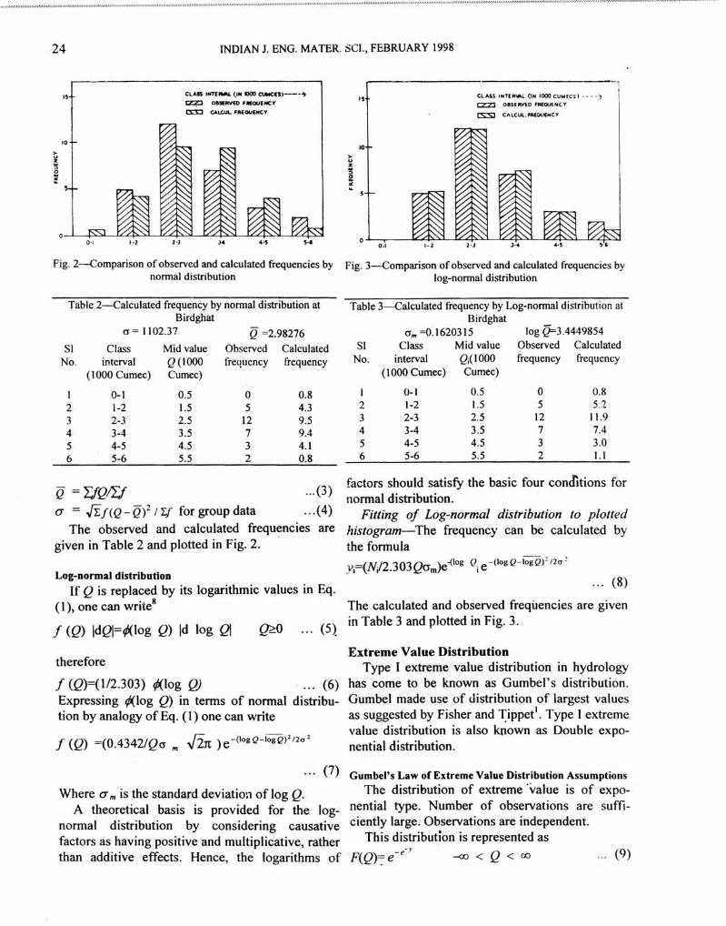
Table 2-Calculated frequency by normal distribution at Table 3-Calculated frequency by Log-normal distribution atBirdghat Birdghat

o = II 02.37 Q =2.98276 crm=O·1620315 log Q=3.4449854

SI Class Mid value Observed Calculated Sl Class Mid value Observed Calculated

No. interval Q(1000 frequency frequency No. interval Qi(IOOO frequency frequency

(1000 Cumec) Cumec) ( I000 Cumec) Cumec)

I 0-\ 0.5 0 0.8 I 0-1 0.5 0 0.8

2 1-2 1.5 5 4.3 2 1-2 1.5 5 5.2

3 2-3 2.5 12 9.5 3 2-3 2.5 12 11.9

4 3-4 3.5 7 9.4 4 3-4 3.5 7 7.4

5 4-5 4.5 3 4.1 5 4-5 4.5 3 3.0

6 5-6 5.5 2 0.8 6 5-6 5.5 2 1.1

•• CLASS IHTE ••••• tiN 1000 c:tAotC(S)---~.,tz:iP OBaRY£O '.auINCYcs:D CALC.UL ,IJt:£OUEHtV

'0

Fig. 2-Comparison of observed and calculated frequencies bynormal distribution

...(3)Q =I/QIL/a = Jf.f(Q - '0)2 ILf for group data ... (4)

The observed and calculated frequencies aregiven in Table 2 and plotted in Fig. 2. .

Log-normal distributionIf Q is replaced by its logarithmic values in Eq.

(1), one can write"

CLASS IHTE""'-l OH 1000 cua.trcs) . - - -)c::z::z] OISULVIO FA£out He y

c:s::sJ CALeUl. Ht(OUEHCY

'5

>-oz

~"."

Fig. 3-Comparison of observed and calculated frequencies bylog-normal distribution

factors should satisfy the basic four conditions fornormal distribution.

Fitting 01 Log-normal distribution to plottedhistogram-The frequency can be calculated bythe formula

.=(JI.T./23031kT )e-{log Q.e-(logQ-IOgQ)'f2a'y, lV,. ~Vm ,

... (8)

1 (Q) IdQI=¢(log Q) [d log QI ~OThe calculated and observed frequencies are givenin Table 3 and plotted in Fig. 3.... (5)

therefore

1 (Q)=(1I2.303) ¢(log Q) .... (6)Expressing ¢(Iog Q) in terms of normal distribu-tion by analogy ofEq. (1) one can write

1 (Q) =(0.4342IQcr m .Ji1t )e-(logQ-logQ)'/2a'

Where a m is the standard deviation of log Q.A theoretical basis is provided for the log-

normal distribution by considering causativefactors as having positive and multiplicative, ratherthan additive effects. Hence, the logarithms of

Extreme Value DistributionType I extreme value distribution in hydrology

has come to be known as Gumbel's distribution.Gumbel made use of distribution of largest valuesas suggested by Fisher and Tippet'. Type I extremevalue distribution is also known as Double expo-nential distribution.

(7) Gumbel's Law of Extreme Value Distribution AssumptionsThe distribution of extreme 'value is of expo-

nential type. Number of observations are suffi-ciently large. Observations are independent.

This distribution is represented asF(Q)~e-e-r -00 < Q < 00 ... (9)

YADAV & PANDE: BEST FITTED DISTRIBUTION FOR ESTIMATION OF FLOOD

Where y=a (Q-u)For a particular return period T, this equation

can be written as

Yra(Qr-u) ... (10)where, Qrestimated discharge for return period Tand

YT = -In[ln F(Q)] ... (11)The value F(Q) is taken to 'be the probability P ofa variate qsQ and this is equal to (1-1/1).Where T is the return period.Thus the value YT=ln*ln T/(T-I) ... (12)For estimation of parameters a and u of this,method of probability paper, method of momentand maximum likelyhood (MLH) method, ap-proximate MLH has been used and given in Table4 and the comparison between MLH and approxi-mate MLH method is given in Table 5.

Histogram for extreme 'value distribution(Gumbel distribution) by probability paper

Table 4--Values of a and u by various methods

Name of Para- Probabi- Method of MLH Approxi-river meter lity paper moment method mate MLH

River a Ll4x 10.3 1.31 x I 0.3 L29x10·3 L29xJO·3Rapti

at u 2574 2606 2569 2406Birdghat

Table 5--Comparison between a and u between MLH andapproximate solution of MLH method at various sites

Name of River Parameter MLH ApproximateMLH

1.29x10.32406

7.16xl0-41603

1.76xlO·26429

River Rapti aat Birdghat uRiver Tons a(Vr.rshney) uRiver Sabarmati aat Dharoi u(Panchang &_A~arwal)

1.29xlO-3

25697.319x 10-4

15801.76xlO-2

6429

Table 6--Calculated frequency by Gumbel distribution atBirdghat

(J = 1102.37yn=O·5353u=2450.47

Class interval Mid value Q(1000-Cumec) (1000 Cumec)

Q=2.98276CTn=I.1086

a=0.00IOO565Observed Calculatedfrequency frequency

25

method-To prepare the histogram, the calculatedfrequency is given by

Y - N -a(Q,-u) _e-a(Qi-UJj - jae " e ... (13)

Gamma Distribution with 2 ParameterGamma Probability density functions can be

classified as Gamma Probability density functionwith one, two or three parameters. The function

O<Q<co ... (14)

is the two parameter Gamma probability function,where a is known as shape parameter and fJ isknown as scale parameter.

The value of a and fJ in terms of Q and a aregiven as

( \5)

Histogram for Gamma DistributionParameters

The calculated frequency is given byy;=(N; /j5'ra) Qt-1e-Q;/f)

The calculated frequenciesand are shown in Fig. 5.

with Two

... (16)are given in Table 7

Table 7-Calculated frequency by Gamma with 2-parametersdistribution at Birdghat

(J =1102.37; QAVG=2.98276; 1l=407.42; a=7.321"'7;fa=720

Class interval Mid value Qi Observed Calculated(1000 Cumec (1000 Cumec) frequency frequency

0-1 0.5 0 0.11-2 1.5 5 6.22-3 2.5 12 11.43-4 3.5 7 7.44-5 4.5 3 2.95-6 5.5 2 0.8

CLASS IHURW4. (IN 1000 CU.IC:S)--~

~ "",a,,,o flllOUONCY

cr:n CALCUL. fAEQV£HCY

0-1 0.5 0 0.21-2 1.5 5 5.62-3 2.5 12 10.7 0

3-4 3.5 7 7.2 o. I ·f 2" '-4 4-5

4-5 4.5 3 3.2 Fig. 4-Comparison of observed and calculated frequencies by5-6 5.5 2 1.3 Gumbel distribution

INDIAN J. ENG. MATER. SCI., FEBRUARY 1998

r-~----------------------------IS

CLASS ••nAVAL (IN fOeo-CUMtCS}-----)

tzZl OeSElW£1J FRtu\JEM..Y

~ CALCUl. FREQUENCY

10

01

Fig. 5---Comparison of observed and calculated frequencies bygamma 2-para distribution

Table 8---Calculated frequency by Pearson Type IIIdistribution at Birdghat

o =1102.37; Q =2.98276; P=377.62;

u=8.52",9; ru=40320

Class interval Mid value Qi Observed Calculated(1000 Cumec) (1000 Cumec) frequency frequency

0-1 0.5 0 0.11-2 1.5 5 3.82-3 2.5 12 10.33-4 3.5 7 8.84-5 4.5 3 4.25-6 5.5 2 1.4

Pearson type III DistributionThe function

h(q)=(ll f3 ara)(q-rt']e,(q,r) IP ... (17)fa is the three parameter probability densityfunction. The parameter r is known as locationparameter. In hydrology for frequency distribution,the use of Gamma distributions with three pa-rameters becomes very common in the form ofPearson Type III distribution.

Pearson" has derived a series of probabilitydensity function to fit virtually any distribution.They have been widely used in practical statisticalwork to define the shape of many distributioncurves. Pearson Type III distribution is a specialcase of this distribution which is often used inhydrological frequency analysis. In this theSkewness coefficient is given by

r,=L( Qj_Q)3/(N_I)a3 ... (18)

And the value of a, 13 and r in Eq. (17) is given bya=4Ir/ (19)l3=cr r]/2 (20)r=Q-(2crlr]) (21)

C.LASS INTERVAl.. <-IN IOOOClWCU) ---- ...•

tz::3 OBSERVED FREauENCY

~ CAlCUl. ~EQVENCY

>-

"z...2if

.-1

Fig. 6---Comparison of observed and calculated frequencies byPearson III distribution

Table 9-Results of Chi-square test on various distributionsof river Rapti at Birdghat

Name of Distribution Chi Square-x2 for 5% level

(NDF=2) (X ~ =5.99)1.280.230.32

NormalLog-normalGumbel (Probability-Papermethod)Gamma with 2-parametersPearson Type III

0.811.02

Testing of the DistributionsTo select a particular distribution for the pur-

pose of prediction of future floods, tests of thegoodness of fit have been done. The Chi-SquareTest of fit is commonly used.

The Chi-Square Test-It has been shown thatthe Chi-Square parameter

2 ""k 2X = L...i~](bi - Cj) I c]

whereb,=number of observations actually in a given

class intervalc=Expected number of observations in a given

class intervali=1, ... k=class interval covering the range of

data.The Chi-Square test prescribes the critical value

of X2 for a given significance level a, so that for X2< X ~ the null hypothesis of a good fit is accepted,

otherwise for X2 ;?: X ~ , it is rejected.

... (23)

Y ADA V & P~DE: BEST FITTED DISTRIBUTION FOR ESTIMATION OF FLOOD 27

In general, the number of class interval k shouldbe greater than 5 and the expected values ofabsolute frequencies should be Cj > 5. If theparameters of distribution function estimated fromthe sample data has a number h, then the number ofdegree of freedom N.D.F=k-h-l. The values of x ~can be obtained for a given N.D.F at a particularlevel of significance (a.) usually taken as 5% fromthe standard text in statistics. Values of "l calcu-lated are listed in Table 9.

ConclusionIt can be seen from Table 9 that all the theoreti-

cal distribution pass the test of acceptance. TheLog-normal distribution in eaoh of these tests giveslowest value as compared with other distributions.Also from perusal of histograms (Figs 2-6), Lognormal distribution is best fitted.

Hence, Log-normal distribution method can beinferred to be the best distribution for calculationof future floods at various sites for river Rapti and

its tributaries and other river systems in Tarairegion of Eastern Uttar Pradesh.ReferencesI Fisher R A & Tippet L H C, Limiting forms of the

frequency distribution of the smallest and largest membersof a sample. paper presented at 24th Annual Convention ofPhil. Soc., Cambridge, UK, 1928.

2 Gumbel E J, Statistics of extreme values (ColumbiaUniversity Press, New York), 1958.

3 Panchang G M & Aggarwal V P, Peakflow estimation bymethod of maximum likelihood (Tech Memo, CWS Re-search Station, Poona, India), \ %2.

4 Pearson K, Tables of the incomplete gamma function(Cambridge University Press, UK), 1921.

5 Varshney R S, Engineering hydrology (Nemchand &Company, Roorkee, India), 1979.

6 Yadav R, Flood problems and characteristics of riversystems in Tarai region of eastern Uttar Pradesh. Ph.DThesis, Madan Mohan Malviya Engineering College,Gorakhpur, 1994.

7 Yadav R & Pande B B L, Indian Water Works Assoc. 28(\996) 93.

8 Yevjevich V, Probability and statistics in hydrology(Water Resources Publication, Fort Collins, Colorado,USA),1972.