BESTAVAILABLE COPY

g19 1 o &Oo

UNCLASSIFIEDSIECURITY CLASSIFICATION OF THIS PAGE

FomAp~roved

REPORT DOCUMENTATION PAGE OnSNo. 0 -0;

la. REPORT SECURITY CLASSIFICATION lb RESTRICTIVE MARKINGSUNCLASSIFIED

2a. SECURITY CLASSIFICATION AUTHORITY 3 DISTRIBUTION/AVAILABILITY OF REPORT

2b. IDECLASSIFICATION IDOWNGRADING SCHEDULE Approved for public release; distribution unlimited

4. PERFORMING ORGANIZATION REPORT NUMBER(S) 5 MONITORING ORGANIZATION REPORT NUMBER(S)

HDL-TR-2139

6a. NAME OF PERFORMING ORGANIZATION 6b. OFFICE SYMBOL 7a NAME OF MONITORING ORGANIZATION(if applicable)

Harr Dimon Labratrie SLCHD-ST-SA

6r_ ADDRESS (City; State, and ZIP Code) 7b ADDRESS (City, State, and ZIP Code)

2800 Powder Mill RoadAdelphi, MD 20783-1197

Be. NAME OF FUNDING/SPONSORING Bb OFFICE SYMBOL 9. PROCUREMENT INSTRUMENT IDENTIFICATION NUMBERORGANIZATION (If al icable)

U.S. Army Laboratory Command AMSLClot ADDRESS (City, State, and ZIP Code) 10 SOURCE OF FUNDING NUMBERS

PROGRAM PROJECT TASK LWORK UNIT2800 Powder Mill Road ELEMENT NO NO. NO 1CCESSION NO.Adelphi, MD 20783-1 145 P611102.H44 AH44

11. TITLE (Include Security Classification)

Rapid Backscatter Simulation Techniques for Detailed B-Spline Target Models

12. PERSONAL AUTHOR(S)Karl D. Reinig

13a. TYPE OF REPORT 13b. TIME COVERED 14 DATE OF REPORT (Year, Month,Day) S. PAGE COUNTFinal FROM Oct 85 TO July87 December 1988 57

16. SUPPLEMENTARY NOTATION

HOL project: AE1814, AMS Code: 6111 02.H4400

17. COSATI CODES 1 SUBJECT TERMS (Continue on reverse if necessary and identify by block number)FIELD GROUP SUB-GROUP B-splines, radar backscatter, target models, backscatter simulation target en-12 01 coun*9r, geometric optics17 09

19. ABSTRACT (Continue on reverse if necessary and identify by block number)

The report describes a method for rapidly evaluating the simulated radar backscatter signatures of B-spline targetrlodels moving relative to a r3urce/receiver. A geometric optics approach is used to estimate the radar return from acomplex target surface described by a bicubic B-spline mesh. The method exploits the second-order continuity of bicubicB-spline surfaces to reduce the problem of finding all the specular points associated with each new trajectory position tothat of tracking the motion of existing points. In particular, it is shown that the locations of the annihilations and creationsof specular paths may be predicted for an entire trajectory, eliminating the need to search the whole surface for specularpoints as the target moves in relation to the sourcetreceiver. The method is shown to work for the multiple-bounce case aswell. The report contains several recommendations for further exploitation of the properties of B-spline surfaces for thetracking of specular points.

ZO. DISTRIBUTION /AVAILABILITY OF ABSTRACT 21 ABSTRACT SECURITY CLASSIFICATIONO UNCLASSIFIEO/UNLIMITED 0 SAME AS RPT Q DTIC USERS UNCLASSIFIED

22a. NAME OF RESPONSIBLE INDIVIDUAL I22b TELEPHONE (Include Area Code) 22t. OFFICE SYMBOLKarl Reinig (202)394-3140 SLCHD-ST-SA - ° -

DD Form 1473, JUN 86 Previous editions are obsolete. SECURITY CLASSIFICATION OF THIS PAWi F

1 UNCLASSIFIED

JAN 6 1988

A

Contents

1. Introduction 51.1 Problem Scenario .............................. 51.2 A Useful Backscatter Modeling Technique .............. 71.3 Surface Modeling with B-splines ................... 8

2. Geometric Optics Approach Using B-splines 112.1 Single-Bounce Return ........................... 112.2 Specular Paths ................................ 132.3 Finding Twinkles ............................... 182.4 Birthing Specular Paths .......................... 192.5 Rotation of Coordinates .......................... 21

3. Extension to Multiple Bounces 233.1 nth Order Specular Points ......................... 233.2 The Bistatic Bounce ............................ 243.3 The nth Order Bounce ........................... 263.4 Example of Savings Using Multiple-Bounce Twinkles ..... .28

4. Algorithm Development and Examples 304.1 Introduction .................................. 304.2 Program Flow ................................. 304.3 Another Single-Bounce Example ..................... 324.4 Missing a Twinkle ...... ........................ 344.5 Double-Bounce Example ......................... 35

5. Proposed Additional Research 375.1 Introduction .................................. 375.2 Efficiently Searching for Twinkles and Initial Specular Points 375.3 Specular Paths as Roots of Polynomial Surfaces ........ .. 405.4 Twinkle Search Through Recursive Subdivision ........ ... 425.5 Inclusion of Surface Discontinuities .................. 43

5.6 Multiple Bodies and Shadowing ..................... 45

5.7 Experimental Validation and Comparison .............. 45

6. Summary 47c¢:n io f4

Distribution 57

L .57 . . ..

3 Avilc-, .. . ... .:

-n t ial

Appendices

A. Newton Step for the Location of a Specular Point on aB- Spline Surface 49

B. Newton Step for the Location of Twinkles 51

C. Taylor Coefficients at a Twinkle in the Rotated Frame 53

Figures

1 Target encounter scenario ..................... 52 Specular return geometry ..................... 113 Initial specular point ........................ 154 Trajectory partitioned by twinkles ..................... 155 Tracking the initial specular point ..................... 166 After birth of two specular paths ...................... 167 After annihilation of two specular paths ................. 178 Final specular plot ................................ 179 Distance surface ....... .......................... 2010 Rotation angle for zero curvature ..................... 2211 Multiple-bounce return ............................ 2312 Rays emanating from a surface ....................... 2513 Bistatic bounce ......... ......................... 2614 Double bounce .................................. 2715 Simple flow chart of algorithm for tracking specular points. 3116 Twinkles and initial specular points ................... 3317 Specular point paths .............................. 3318 Double-bounce twinkle ....... ...................... 3619 Double-bounce specular point paths ................... 36

4

1. Introduction

1.1 Problem Scenario

The expanding technology base exploiting millimeter and near-milli-meter electromagnetic waves has greatly enhanced the ability of re-mote sensors to detect and identify complex targets of interest. Theenhancement is especially significant when the target is obscured byfog, clouds, or smoke which can render infrared and optically basedsensors useless. As a result, a large number of sensors operating atmillimeter and near-millimeter wavelengths have been produced forsuch applications as identification of targets, terminal guidance, andfuzing. Accordingly, the need for efficient and informative simulationtechniques for these high-frequency sensors has also risen. Considerthe scenario depicted in figure 1.

A source/receiver (S/R) moving along some trajectory illuminatesa target of interest. It is desired to estimate the return from the targetas the S/R moves along the trajectory. Notice that whether figure 1describes a target detection/identification problem or the terminalphase of a guided munition is mostly determined by the trajectorybeing considered. A backscatter simulation technique which placesfew or no restrictions on the paths of the trajectories to be simulated

Figure 1: Target encounter scenario.

5

could therefore find use in all phases of seeker munitions studies. Inaddition, of course, the relative motion between the S/R and thetarget could be due strictly to the motion of the target. Thus thescenario could also include the return from passing targets. It willbe assumed that the return should be calculated about a thousandtimes per meter of trajectory. The reason for mentioning this detailhere is to introduce early the impact of the trajectory on any practicalmodeling method. In particular, this study attempts to include thetrajectory into the structure of the problem, as opposed to simplyconsidering the trajectory as a sequence of points at which to evaluatethe return.

This report begins with a brief review of a modeling method devel-oped at the Harry Diamond Laboratories for the computer simulationof fuze/air-target encounters. The simulation technique uses a com-posite of simple analytic structures (cones, spheres, flat plates, etc)to model the surface of a target of interest. A geometric optics as-sumption is then used to estimate the expected amplitude and phaseof the return as the S/R moves along the trajectory of interest. Thecurrent study makes use of bicubic B-spline patches to describe ar-bitrary complex targets in greater detail. Using the geometric opticsapproach for estimating the target return, the backscatter problembecomes one of finding all the specular points of such an arbitrarysurface with respect to the S/R location.

The main portion of this report describes a method for exploitingthe continuity of the resulting surface model to reduce the problemof finding all the specular points associated with each new trajectoryposition to that of tracking the motion of existing points. In particu-lar, it is shown that the locations of the annihilations and creations ofspecular paths may be predicted for an entire trajectory, eliminatingthe need to search the whole surface for specular points as the targetmoves in relation to the S/R. It is further shown that the same tech-nique can be extended to include so-called multiple-bounce return, inwhich it is assumed that the signal is reflected about the surface two ormore times before returning to the receiver. The general flow of sim-ple algorithms for the implementation of the new strategy is describedand the results of example runs displayed. The examples point outpotential robustness problems with the simplistic algorithms, prob-lems which are not inherent in the modeling method itself. The finalsection of the report outlines potential solutions to these problems aswell as extensions to the model. The potential solutions and exten-

6

sions are presented as part of the suggested areas of further researchand include

" the potential for further exploitation of the properties of bicu-bic B-spline surfaces to increase the robustness of the speculartracking algorithms,

* extensions to include surface discontinuities,

" extensions to include multiple bodies and shadowing, and

" experimental validation and comparison with other methods.

1.2 A Useful Backscatter Modeling Technique

Methods for developing radar backscatter models of air targets suit-able for computer simulation of radar-fuze/air-target encounters aredescribed by Dammann [1]. The models are developed in three steps:

First, the target is approzimated by an ensemble ofsimple geometric shapes such as ogives, cylinders, flatplates, and ellipsoids. Second, the specular point (the pointwhere the surface is perpendicular to the incident rays) islocated on each shape. All the return is assumed to comefrom these specular points, and the strength of the returnfrom each point is assumed to depend on the local curva-tures of the surface at that point. Third, the returns fromall specular points are summed vectorially to yield the totaltarget return. [1]

This modeling method has proved to be very useful both for pre-dicting the backscatter characteristics of interest in fuze design andfor the simulation of fuze processors. In particular, because the modelprovides actual Doppler voltage waveforms, the computer-generated

waveforms can be fed directly into actual fuze processors to predicttheir response.

The target modeling technique described above has been particu-larly successful in the air-target encounter scenario partially becauseof the relative simplicity of the shapes of most aircraft. In many cases,between 10 and 20 primitive analytic shapes are all that are necessaryto capture the essential shape of a particular aircraft. As the targets

of interest become more complex or the desire to match their surfacemore accurately increases, the use of simple analytical shapes to de-

scribe the target surface often becomes impractical. Tensor-product

7

piecewise polynomial surfaces are a simple means of describing com-plex surfaces, and as such, present a practical way to extend thegeometric optics approach to include targets of increased complexity.

1.3 Surface Modeling with B-splines

In this paper it is assumed that a three-dimensional vector function

R(u,v) exists which describes the target surface of interest; that is,given a particular choice of u and v, R(u,v) represents the x-, y-, andz-coordinates of a point on the target surface. It is further assumedthat over the entire domain of R (call this U x V) the partial derivativevectors

0/+JR(u, v)Ouiev.i(1

exist and are continuous for i ± j <5 2. B-splines can be used to con-vert a patchwork of data points into just such a function. For themajor results of this paper it is the second-order continuity of thesurface which is exploited to reduce the backscatter simulation time,and an understanding of B-splines is really not necessary. However,the following brief discussion may be helpful. (The reader interestedin the details of B-splines in general is encouraged to study de Boor'sbook A Practical Guide to Splines [2] or, for a quicker look, see Gordonand Riesenfeld [3], Cox [4], or Amos [5].)

The mathematical term "spline" originates from the mechanicalspline used by draftsmen to trace out smooth curves. When thinstrips of wood or metal are pinned at strategic locations on the draft-ing board, the material takes on a shape to minimize its internal stressand gives a generally pleasing interpolant to the data. If the drafts-man is not pleased with the resulting trace, the number of pinningpoints and their locations may be altered until the desired shape isformed. Piecewise polynomial functions are the mathematical mate-rial of choice for fitting smooth curves through or near a given set ofdata. The term "piecewise" refers to breaking up the entire curve intosections of low-order polynomials (most often cubic). The sections arejoined at "knots" so that appropriate continuity is maintained. Theterm "B-spline" refers to a special set of piecewise polynomial func-tions which form a basis for all piecewise polynomials having a givenknot set and continuity constraints at the knots. As an example, thecubic B-spline basis functions with uniformly spaced knots having ze-roth, first, and second derivative continuity at each of the knots maybe written as

8

Bi(z) = (I - z)6,

B 2(z) = (3z 3 - 6z 2 +4)/6,B3(z) = (-3z3 +3z 2 +3z+1)/6,

B 4 (z) = z3/6.

Note that a linear combination of the functions above can be used toconstruct any desired cubic polynomial. Now suppose that we havea rectangular mesh of points which we would like to use to describea surface. The mesh can be used to form a tensor product surfaceusing the same basis functions. Consider the behavior of the following

function:4 4

Rk,1(Uv) = Bj(u)(Aj+kj+j)B,(v),i--1 j=1

where Ai+k,j+/ are three-dimensional vectors of finite length and u andv are real numbers ranging from 0 to 1. Rkj(u,v) is simply one way ofwriting a bicubic B-spline surface defined over a uniform rectangularknot set for the k,lth patch of the quilt of data points. Clearly, forany fixed values of k and 1, and for all u and v E (0, 1), the variouspartial derivatives of equation (1) are continous functions of u and vfor all positive integers i and j. It is also easy to verify that all thezeroth, first, and second partial derivatives with respect to u and vare continuous across neighboring values of k and 1. For example,

O2RkL(uV) 4 OB, () OBj(v)Ou ~Fv E (A~ i+k,+l)Ouvi=1 j=1 OIO

1/4 {-(1 - u)2[_(1 - v) 2 Ak+,,I+l + (3v 2 -4v)Ak+1:+2

+(-3v2 + 2v + 1)Ak+1,1+3 + v2Ak+l,+ 41

+(3u' - 4u)[-(l - v) 2 A:+2,1+1 + (3v2 - 4v)Ak+,,+2

+(-3v2 + 2v + 1)Ak+2,,+3 + v2 Ak+ 2,1+4)2]+(-3u + 2u + 1)[-(1 - v) Ak+3,1+1 + (3v -4v)Ak+3,+ 2

+(-3V2 + 2v + 1)Ak+a,/+3 + V2Ah+3,1+4]

+(U2)(_(1 - v)'Ak+4,+1 + (3v 2 - 4v)Ak+4,,+2

+(-3v2 + 2v + 1)Ak+4,t+3 + v2Ak+4,1+4},

9

from which it is an easy check that

192 Rk,(U, 0) 1/4 {-(1 - u)[Ak+l1+1 + A+1,+31

+(3U 2 - 4u)[Ak+2,1+1 + Ak+2 ,1+3]

+(-3u2 + 2u + 1)[Ak+3,1+I + Ak+3,1+3I

+(u2)[Ak+ 4,1+1 + Ak+4,1+31}0 2 Rk,1..(U, 1)

OuOv

While many surface modeling methods offer smooth surfaces, the B-spline surface in general has three major properties which make itparticularly well suited for surface modeling. The first is that the sur-face passes near (in a sense that will not be elaborated here) the pointsAij. This allows the modeler to choose a mesh of points which gen-erally describes the desired surface (much like a planar facet model)and then observe the resulting surface. As might be expected, themore points that are used to define the surface, the closer the sur-face will pass to the points. The second major property is the localinfluence of the points Aij; that is, a change in the position of thepoint Aij only changes the surface near the point. The local natureof the spline allows the modeler to move points around to improve thesurface in a particular area without modifying the rest of the model.The third major property, closely related to the first, is the variation-diminishing property of B-splines. Loosely speaking, the variation-diminishing property guarantees that any plane will cut through athree-dimensional B-spline curve no more times than it does a linearinterpolant to the original data points.

It is the second-order continuity of the surface which is exploitedfor the main results of this paper. Since many other methods exist forrepresenting smooth surfaces, the main results are more general thanjust for B-spline surfaces. However, mostly because of the previouslystated B-spline properties, the surfaces exemplified in this report areall based on B-splines. In addition, a large portion of the suggestedfurther research is aimed towards exploiting those properties specificto B-spline surfaces.

10

2. Geometric Optics Approach Using B-splines

2.1 Single-Bounce Return

The geometry of the specular return problem from a single patchof an arbitrary B-spline surface is shown in figure 2. Rt(A) is thecurrent position of the projectile along a linear trajectory, R,(u, v)

describes the target surface as a function of the two parameters u andv, and G(u, v, A) is the difference between the two vectors RI(A) andR,(u, v). It is assumed throughout the analysis that the projectile hasan unobstructed view of the surface being considered (the problem ofshadowing is ignored and addressed only in the section on suggestedfurther research). A necessary and sufficient condition for a point onthe surface to be a specular point relative to the position Rt(A) is thatthe 12 norm of G(u, v, A) be either a local maximum or minimum withrespect to the two target surface parameters u and v. Finding all thespecular points of a given surface (for a given trajectory position) istherefore the same as finding all u and v that satisfy the two nonlinearequations

F,(u,v, A) 8 IG(uv, A)11 2 -0 (2)Ou

and

F2(u,v,A) - 9IG(u,, A) 11 2 -. (3)

If R(u,v) is given by a tensor product of cubic B-splines on a uni-form grid, both Fi(u, v, A) and F2(u,v, A) may be written explicitly

/, u vAR, (U, Vz Rt( A

Y

Figure 2: Specular return geometry.11

in terms of u and v. However, the u and v which solve equations (2)and (3) (call them u* and v*) cannot be found explicitly, since Fl(u, v)is a bivariate polynomial of degree five in u and six in v, while F2 (u, v)is a bivariate polynomial of degree six in u and five in v. In generalthen, solving equations (2) and (3) for u* and v* requires a numer-ical technique. Simple application of Newton's method for nonlinearequations will find solutions to (2) and (3) provided the search is be-gun "close enough" to (u*,v*). The question of how close is closeenough is a complex one which ultimately depends on the variationof the surface being considered. An explanation of Newton's methodand algorithms which incorporate the method may be found i. mostoptimization texts including Luenberger [6]. The essential step is tosolve the following linear system of equations:

J(u,v)S = F(u,v), (4)

where F(u,v) is the 2 x 1 vector [F1(u,v),F 2(u,v)], J(u,v) is the2 x 2 Jacobian of F(u, v) with respect to u and v, and S is the 2 x 1vector for the new step in u and v. A derivation of the Newton step

for the location of a specular point on a B-spline surface may be foundin appendix A. It is easy to see that for the bicubic B-spline surfacebeing considered, the elements of J(u,v) are continuous functions ofu and v; that is, all second-order derivatives of G(u,v) exist and arecontinuous functions of u and v.

Using Newton's method alone, it would be possible to thoroughlysearch each B-spline patch for specular points, keeping track of theirpositions and local principal radii of curvatures for use in the geomet-ric optics estimation of the return from the composite model. Theprocedure would have to be repeated for each new position along thetrajectory. To get a feel for the time which may be required for a sin-

gle simulation, suppose a target were being modeled by B-splines overan 80 by 50 knot grid (4000 patches, give or take a few end conditions)and that it were possible to thoroughly search 100 B-spline patchesper second. The specular return from the target could be calculatedin approximately 40 s for one point along the trajectory of interest.Now suppose further that we are interested in a 10-m trajectory tobe sampled at 1-mm increments (not an unlikely requirement whenworking with millimeter waves). The simulation of the signature for

the single trajectory would take approximately 400,000 s, or a littleover four and one half days. Admittedly, other techniques could prob-ably be used to cut down on the time required to search the composite

12

model for specular points. (Methods based on recursive subdivision ofthe target surface using, for example, the Oslo algorithm [7 should beconsidered.) However, any method which searches all 4000 patches foreach position of the trajectory is going to be very computer intensive.

2.2 Specular Paths

Whether gradient techniques such as Newton's method are fast or not,they can give important insight into the motion of specular points. Letthe current trajectory position (Rt) of figure 2 vary linearly betweenthe two endpoints Rt 1 and Rt 2 as

Rt(A) = ARt2 + (1 - A)Ri. (5)

For the surface considered here, the distance function G(u,v,A) isa continuously differentiable function of u, v, and A. Suppose thecoordinates of a specular point are known for a particular value ofA and we wish to observe the motion of the specular point as Achanges. The following argument is a trivial extension of that givenby Longuet-Higgins for a time-varying analytic surface [8]. The con-ditions for a specular point are given by equations (2) and (3). Takingthe differential of equations (2) and (3) with respect to u, v, and Ayields

2 I1G(u, v, A)112 d 02 l)G(uvA)1J2 d + 8 IIG(u ,, A)112 dA = 0,1u2 OuOv OuOA

2 IG(uvA)12 d 2 1G(u, v, A)1 2 dv + 2 IG(uVA)12 dA = 0,1u9v u+ 0v 2 Ov9A

which may be rewritten in matrix form as[du IdA 1 r821IG(UV.&)II 2 1dv/dA j I G(uvA,) 2 ' (6)

where J(u,v,A) is the same 2 x 2 Jacobian used in the Newton'smethod search (with its dependence on A explicitly noted). Sincethe elements of J(u, v, A) are continuous functions of u, v, and A, ifJ(u, v, A) is nonsingular, du/dA and dv/dA will both be finite, whichimplies that the changes in u and v can be kept as small as desiredby choosing the change in A small enough. Longuet-Higgins [8] refersto the vanishing of the determinant of J(u, v, A) as a twinkle. Thephysical significance of this result is that as the source/receiver moves

13

across a second-order continuous surface, specular points cannot sud-denly appear or disappear unless J(u,v, A) is locally singular. Theobservation that specular points move in continuous paths brokenonly wheu J(u, v, A) is singular leads directly to the following conclu-sion. If, for any given trajectory, it were possible to determine all thepoints (u, v, A) for which J(u, v, A) is singular, it would no longer benecessary to search the entire surface for specular points at differentpositions along the trajectory. It would only be necessary to find allthe specular points corresponding to one trajectory position (tt forexample) and then track their motion, picking up or losing specularpaths only at twinkles. It is shown in section 2.4 that the annihila-tion or creation of specular paths must also occur in pairs; that is, apair of specular paths must run into each other to be annihilated, ororiginate from a single point on the surface to be created.

To get a feel for the potential computational savings to be gainedby first finding the twinkles associated with a particular trajectory,consider the previous example. Suppose that on the average therewere 10 specular points on our surface of 4000 B-spline patches andthat it took about the same amount of time to update the locationof 5 specular points as it did to search an entire patch for specularpoints. Once all the twinkles have been found for the trajectory andthe problem is reduced to a specular tracking problem, it will takeon the average 1/2000 times as long to find each new set of specularpoints; thus, the computational time will be reduced from a little over4-1/2 days to 3-1/3 minutes, plus whatever time it takes to find thetwinkles. Recalling that the search for twinkles is only conductedonce for a given trajectory, we could reduce the computational timerequired to simulate the backscatter from complex targets by two ormore orders of magnitude.

The following example both clarifies how twinkles may be used totrace the motion of specular points along a surface for a given trajec-tory, and motivates the derivations that follow. Figures 3 through 8show the evolution of a specular plot for a simple target surface andan associated trajectory of interest. To keep the example relativelyuncluttered, it is assumed that in addition to having the continuityproperties discussed before, the surface is such that no specular pointslie on its edge for any location along the trajectory. The first step isto find all the specular points associated with the beginning of thetrajectory; in this example, only one such point exists on the surface,as shown by the X in figure 3. The next step is to find all the twinklesassociated with the chosen trajectory and partition the trajectory ac-

14

-FIN1ISH

S TART

------- . .....

.. .. ........

Figure 3: Initial specular point.

FIN1ISH

D

START

..... . . . .. ------1

. ... ... .

Figure 4: Trajectory partitioned by twinkles.

15

.F IN1 ISH

D

FTAR

Figure 5: Tracking the initial specular point.

FIMISH

/TAR T

Figure 6: After birth of two specular paths.

16

FINISH

TART

Figure 7: After annihilation of two specular paths.

IMISH

TAR

Figue 8:Fina speularplot

174

cordingly. In addition it will be helpful to know whether each of thetwinkles represents a birth or a death of a pair of specular paths. Ithas already been shown that at a twinkle the Jacobian which mightordinarily be used to determine the location of the specular pointsbecomes singular, making it difficult to locate specular paths near atwinkle. Fortunately, a solution is available to the problem of predict-ing the motion of specular points near a twinkle, as well as predictingwhether a twinkle represents the birth or death of a pair of specu-lar paths, as shown in section 2.4. Figure 4 shows the partitioningof the trajectory, labeling of the twinkles according to whether theyrepresent births or deaths, and prediction of specular paths near thetwinkles. For all trajectory locations between the origin of the tra-jectory and the first twinkle, it is only necessary to determine themotion of the original specular point (since no new specular pointswill occur anywhere on the surface except at a twinkle). Figure 5shows the motion of the original specular point in the region preced-ing the first twinkle. When a twinkle representing the birth of twospecular paths is reached, the two new paths must be included in theset of specular points to be tracked, at least until the next twinkle.Figure 6 shows the situation after the first twinkle and shortly beforethe second. At that time one of the specular points which originatedat the birthing twinkle was heading for an annihilation with the orig-inal specular point. Figure 7 shows the specular plot at a time afterthe two specular paths collided at the remaining twinkle. For the re-mainder of the trajectory, it is only necessary to track the motion ofthe one remaining specular path, as shown in figure 8. Once again, itshould be pointed out that the 14 by 14 grid of spline patches whichformed the surface in this example was only searched once for the ini-tial specular points and then once again for the twinkles. After that,specular points were simply tracked.

2.3 Finding Twinkles

As shown in the previous section, a necessary condition for the cre-ation or annihilation of a specular path is the vanishing of the determi-nant of J(u, v, A). Denote the determinant of J(u, v, A) as F3 (u, v, A).Then Fs(u, v, A) is given by

F3 (u, v,A) = 2G(u, v, A) 2G(uvA) ( 2 G(u, v,A))218,uvoA), - (7)

18

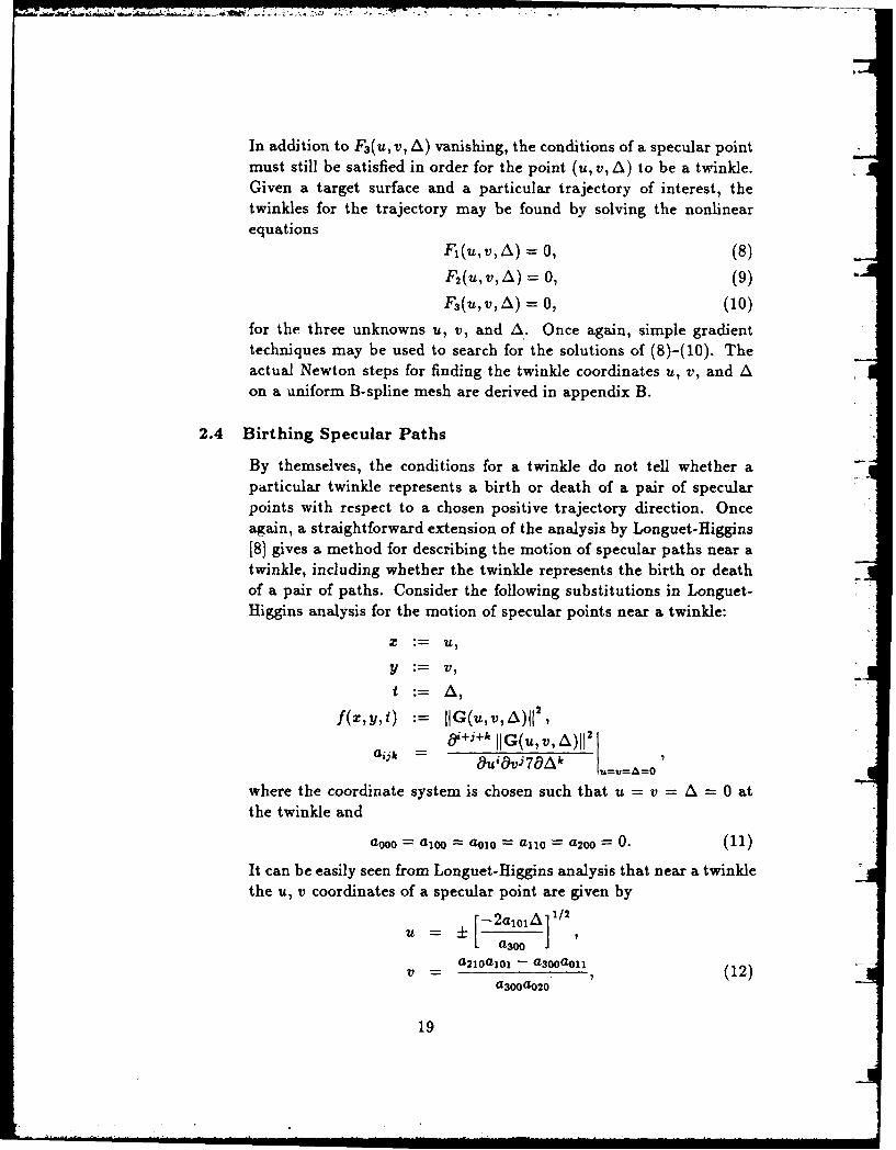
In addition to F3 (u, v, A) vanishing, the conditions of a specular pointmust still be satisfied in order for the point (u, v, A) to be a twinkle.Given a target surface and a particular trajectory of interest, thetwinkles for the trajectory may be found by solving the nonlinearequations

Fi(U1 V, A) = 0, (8)F2(u,v,A) = 0, (9)F3(u,v,A) = 0, (10)

for the three unknowns u, v, and A. Once again, simple gradienttechniques may be used to search for the solutions of (8)-(10). Theactual Newton steps for finding the twinkle coordinates u, v, and Aon a uniform B-spline mesh are derived in appendix B.

2.4 Birthing Specular Paths

By themselves, the conditions for a twinkle do not tell whether aparticular twinkle represents a birth or death of a pair of specularpoints with respect to a chosen positive trajectory direction. Onceagain, a straightforward extension of the analysis by Longuet-Higgins[8] gives a method for describing the motion of specular paths near atwinkle, including whether the twinkle represents the birth or deathof a pair of paths. Consider the following substitutions in Longuet-Higgins analysis for the motion of specular points near a twinkle:

X : - U,

y - V,t :=A,

f(x,y, := I1G(uv, A)112 ,

0 +j+k 11G(u,v, A)112

aijk Ouiov70Ak A=

where the coordinate system is chosen such that u = v = A = 0 atthe twinkle and

ao0 = alo0 = aol0 = all0 = a2oo = 0. (11)

It can be easily seen from Longuet-Higgins analysis that near a twinklethe u, v coordinates of a specular point are given by

= [ -2al°A ,1/2

a,300

a21oalo - a3ooaoll (12)a 30 ao 2o

19

Equations (12) show that if alol/asoo is positive, then two solutionsexist when A is less than zero and no solutions exist when A is greaterthan zero; that is, a pair of specular paths is annihilated. Similarly, apair of specular paths is created when ajoi/asoo is negative. It remains

to determine a transformation of coordinates for which equations (12)hold. Simply choosing the origin of the new coordinate system to bethe location of the twinkle ensures that a000 is equal to zero. It willbe useful here and for analysis to come to consider the surface formedby letting the function (IG(u,v, A)112 be the w coordinate in an or-thogonal u, v, w coordinate frame, as shown in figure 9. For lack ofa better term, this surface is referred to as the "distance surface."The condition for a twinkle may then be interpreted physically as thevanishing of the Gaussian curvature of the distance surface. Or alter-nately stated, at a twinkle, one of the two principal radii of curvatureof the distance surface is equal to zero. The curvature of any smoothsurface, at a given point, in the direction 6u, 6v may be written as(see, among others, Faux and Pratt [9])

,t, = (6U) 2a2oo + (6u)(6v)aio + (6V) 2 a 2o. (13)

Now suppose the coordinates are rotated so that the u-coordinate isaligned with the principal radii of curvature having zero value (sucha direction must exist at a twinkle). Then with 6v - 0, equation (13)yields

0 = (bU) 2a2OO,

IIG(u,, v, A)II 2

Figure 9: Distance surface.

20

JIG(UVIA)I

.... ~ ~ ~ ~ ~ ~ ~ ~ ~ ~ ~ ~ ~ A 112 -,m, ama an illnial i iaml ..

which implies that a200 = 0. It can be seen that the twinkle conditionimplies

a 200 a0 20 - a =l = 0.

Therefore, in the rotated coordinate system, al1o must also be equalto zero and equations (11) are satisfied. Define the new coordinatesU', V1 , and A' by

u = u'cosO-v'sin6+ut.,v = u'sin0+v'cos0+vtw,A = A+t,

where ut,,, vtw, and a, are the original coordinates of the twinkle.Then if 0 is the angle which rotates the original u-axis into the di-rection of zero curvature, the signs of al01 and a300, in the new coor-dinates, will tell whether the twinkle represents a birth or a death.In addition, the motion of the specular points near the twinkle (inthe new coordinates) will be given by (12). The derivation of theequations for a300, a101, a21 0, aoll, and a0 2o in terms of the originalcoordinates and 6 is given in appendix C.

2.5 Rotation of Coordinates

In order to carry out the procedure of the preceding section, it is nec-essary to determine the angle 0 which rotates the original u-directioninto the direction of zero (principal) radius of curvature. DefineU(t) := (u(t),v(t)) to be a curve on the surface R(u(t),v(t)). Itcan be shown (see for example, Faux and Pratt [9], p 112) that fordU/dt to be in the direction of a principal radius of curvature it mustsatisfy the following matrix equation:

[D - r.E]dU/dt = 0

where

[= n. n. aue1[D] = 8uru vn

.r(UV) 82r(us r(.m

au av OU 9V

and n is the local unit normal to the surface. The conditions thatdU/dt point in the direction of a principal radius of curvature andthat the curvature be zero require that

[D]dU/dt= 0. (14) _

21

Ordinarily matrix equation (14) would have only the trivial solutiondU/dt = 0. However, for the case being considered here, the elementsof [D] are the same as the elements of the Jacobian introduced earlier,which has been shown to vanish at a twinkle. Therefore, the twoequations implied by (14) are not independent, and we are free tochoose either as the necessary condition for dU/dt to point in thedirection of zero curvature. The resulting relation is

it/i, = -d 12/duj

or0 = tan-(-dii/dl2 )

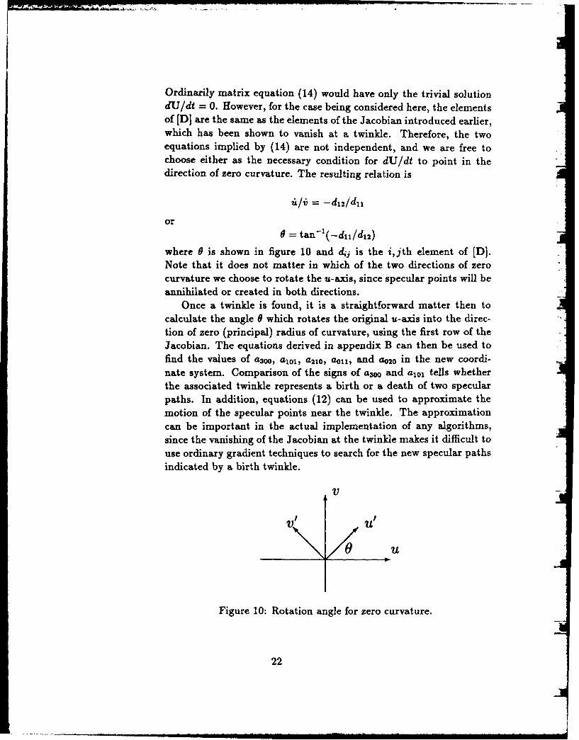
where 0 is shown in figure 10 and di1 is the i,jth element of [D].Note that it does not matter in which of the two directions of zerocurvature we choose to rotate the u-axis, since specular points will beannihilated or created in both directions.

Once a twinkle is found, it is a straightforward matter then tocalculate the angle 8 which rotates the original u-axis into the direc-tion of zero (principal) radius of curvature, using the first row of theJacobian. The equations derived in appendix B can then be used tofind the values of a300, ajo, a2 10 , aoll, and a020 in the new coordi-nate system. Comparison of the signs of a3 00 and al01 tells whetherthe associated twinkle represents a birth or a death of two specularpaths. In addition, equations (12) can be used to approximate themotion of the specular points near the twinkle. The approximationcan be important in the actual implementation of any algorithms,since the vanishing of the Jacobian at the twinkle makes it difficult touse ordinary gradient techniques to search for the new specular pathsindicated by a birth twinkle.

V

Figure 10: Rotation angle for zero curvature.

22

3. Extension to Multiple Bounces

3.1 nth Order Specular Points

Often multiple-bounce return, as depicted in figure 11, produces a sig-nificant contribution to the overall target backscatter. Recall that thegeometric optics approach assumes that the energy emanating fromthe source strikes the target and is then reflected in the same way aswould a plane wave incident on a plane tangent to the surface, or put

even more intuitively, as a ball bouncing off a billiard cushion. Forthe single-bounce return already considered, this implies that energywill only return from locations on the surface for which the local sur-face normal points towards the S/R. However, for complex surfaces,that energy which is reflected by the surface in other directions maystrike another surface location so as to be directed back to the re-ceiver. When the magnitude of the energy returned after multiplebounces is calculated, both the increased distance traveled and the

loss at each reflection serve to diminish the result. For this reason,the single-bounce return is often referred to as the primary or first-order specular return, while the double-bounce return is referred to asthe secondary or second-order specular return (with the obvious nota-tional extension to higher order bounces). The actual target surfacelocations at which the reflections are considered to occur are denotedthe nth order specular points. For many targets of interest, it maybe assumed that the multiple-bounce return is negligible compared to

the single-bounce return. However, if the target surface is assumed tobe highly reflective, the local curvatures of the surfaces at the specular

Source/Receiver

Figure 11: Multiple-bounce return.

23

points small, and the added round trip distance not too large, thenmultiple bounces may occur which have return energy with magnitudeof the same order as the single bounces.

3.2 The Bistatic Bounce

Fortunately, it can be easily shown that the conditions for an nthorder specular bounce are directly related to the total distance of theline segments connecting the source to the receiver via each of the nthorder specular points. In fact, the following result can be stated as animmediate consequence of a weak form of Fermat's principle of optics.

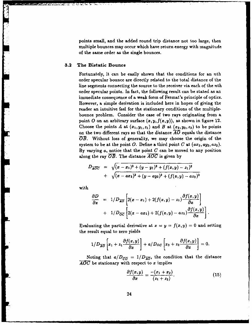
However, a simple derivation is included here in hopes of giving thereader an intuitive feel for the stationary conditions of the multiple-bounce problem. Consider the case of two rays originating from apoint 0 on an arbitrary surface (m, y,f(z, y)), as shown in figure 12.Choose the points A at (zi,yi,zi) and B at (z 2 ,y2 ,z 2 ) to be pointson the two different rays so that the distance A0 equals the distance

OR'. Without loss of generality, we may choose the origin of thesystem to be at the point 0. Define a third point C at (az2 , ay2, aZ2 ).

By varying a, notice that the point C can be moved to any positionalong the ray O--. The distance is given by

D oo = V/(X zi) 2 +(y-y) 2 +(f(zy)_zi)2

+ - az2) 2 + (y - ay2) 2 + (f(xy) - aZ2) 2

with

OD =_____2_ -x)+ ( Z'Y Z)O (,Y

+ 1/DUc[2(x-aX2)+2(f(z,y)-az 2) Y)

Evaluating the partial derivative at z = y = f(x, y) = 0 and settingthe result equal to zero yields

I/D- XI + zI O --Y) +a/Doc X2+Z z9f0.X, Y)

Noting that a/D- = 1/Di-, the condition that the distanceAOC be stationary with respect to z implies

Of(X,y) - -(Zi + (15)Ox (zj + z2 )

24

( 2, ay 2 , az 2 )

xiYlzl)

B (x 2, Y2, z 2)

0 Yx

Figure 12: Rays emanating from a surface.

Repeating for the partial derivative of the distance with respect to yyields 'Of(X, Y) -(Y1 + Y2) (6

S (+ 2 ) (16)Note that equations (15) and (16) are not defined when z, = -Z2.

However the coordinate system could always be rotated so that z1is not equal to z2, allowing us to assume without loss of generalitythat z, does not equal -z2. Equations (15) and (16) imply that twovectors lying in the tangent plane are

T,= (ZI + Z2)i - (XI + X2)k

andT2 = (z1 + z2)j - (y1 + y2)k.

And from the above assumption, T 1 and T 2 form a basis for thetangent plane at 0.

Now consider the conditions for a bistatic bounce. A ray leavingpoint A and striking the surface at 0 will be reflected through C ifand only if it passes through B. Since D- is equal to Dp-, any raystarting at (XI, Yi, z1) and striking the surface at 0 will pass throughthe point (X 2,y 2, z 2) if and only if the ray R, (shown in fig. 13) is nor-

25

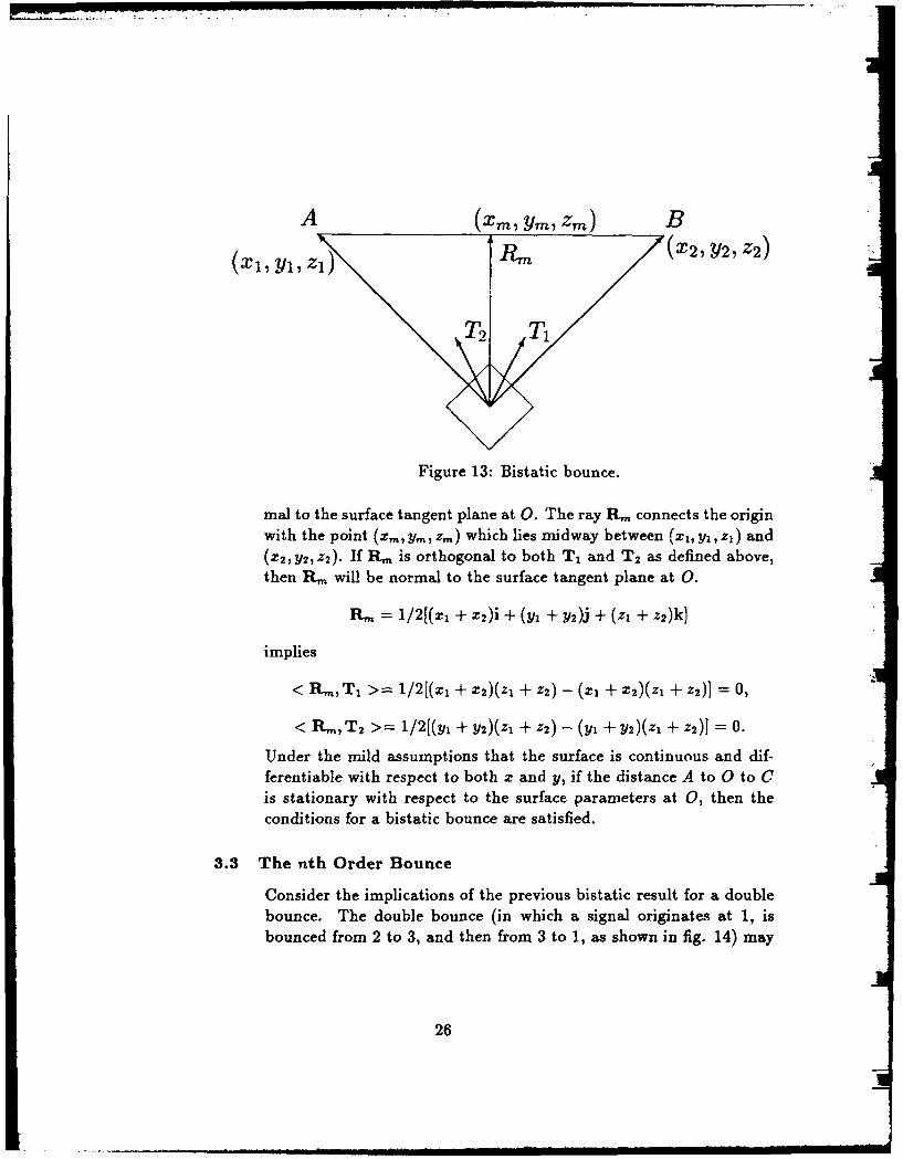
A (Xm, Ym,Zm) B

(X1, 1, 1 I Y7Z - (X21,Y21Z2)

2 T,Figure 13: Bistatic bounce.

mal to the surface tangent plane at 0. The ray Rln connects the originwith the point (,,,, ym., z.) which lies midway between (0, y, z) and(X2, Y2, z2). If R, is orthogonal to both T1 and T 2 as defined above,then Rm will be normal to the surface tangent plane at 0.

Rn = 1/2[(xi + z2)i + (Y2 + Y2)j + (z1 + z2)k]

implies

< R,,T, >= 1/2[(xi + z 2)(zI + z2) - (X1 + X2)(zl + z2 )] =0,

< R.,T 2 >= 1/2[(y, + Y2)(z1 + z2) - (Y1 + Y2)(zl + z2)] =0.

Under the mild assumptions that the surface is continuous and dif-ferentiable with respect to both x and y, if the distance A to 0 to Cis stationary with respect to the surface parameters at 0, then theconditions for a bistatic bounce are satisfied.

3.3 The nth Order Bounce

Consider the implications of the previous bistatic result for a doublebounce. The double bounce (in which a signal originates at 1, isbounced from 2 to 3, and then from 3 to 1, as shown in fig. 14) may

26

1

2

Figure 14: Double bounce.

be viewed as the simultaneous result of two bistatic return problems:i.e., from 1 to 2 to 3 and from 2 to 3 to 1. Both of the bistaticcases must satisfy their respective local stationary conditions, andso the total distance 1-2 + 2- + 1 must be stationary with respectto the four surface parameters used to describe the two reflectingsurfaces. The argument immediately generalizes to any number ofbounces. Thus, just as the single-bounce specular points on a surfacemay be found by searching for stationary points of the distance fromthe source/receiver to the surface (and back if you like), multiple-bounce paths may be found by searching for stationary points of thetotal round-trip distance. Each new bounce simply introduces twonew stationary conditions along with two new surface parameters.The same Newton technique which was used to find single-bouncespecular points may be used to find multiple-bounce specular points(recall that we are ignoring for now the problem of shadowing). Thestationary conditions may be stated in terms of the distances shownin figure 11 as

-= =0 = I - vauj Ovj :

for all j = 1, ... , n. Noting that

9u 1 - 027 Od 0Ouj Ovj

27

whenever i - 1 < j or j i + 2, we get the 2n conditions

O(d, + =~l 0 = (d. + di+,)

Oui Ovi

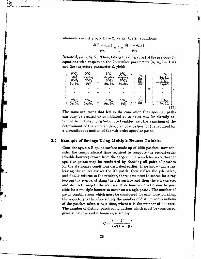
Denote di +di+l by Gi. Then, taking the differential of the previous 2nequations with respect to the 2n surface parameters (ui, vi, i 1,n)and the trajectory parameter A yields

20 G G ' 82 G 2l du2 G1 .2

= u Ou v, -' au.,,Ov 4ulav. dA9U O(92 1 a2t~v a2i~, Bi12 A. 962 2 020 G G2 2 gJ G

a2G 020 82 G 2. y 2alla l aVla Vn v * OUn8V- 8V2 dA - - vOAa

(17)The same argument that led to the conclusion that specular pathscan only be created or annihilated at twinkles may be directly ex-tended to include multiple-bounce twinkles; i.e., the vanishing of thedeterminant of the 2n x 2n Jacobian of equation (17) is required fora discontinuous motion of the nth order specular paths.

3.4 Example of Savings Using Multiple-Bounce Twinkles

Consider again a B-spline surface made up of 4000 patches: now con-sider the computational time required to compute the second-order(double-bounce) return from the target. The search for second-orderspecular points may be conducted by checking all pairs of patchesfor the stationary conditions described earlier. If we know that a rayleaving the source strikes the ith patch, then strikes the jth patch,and finally returns to the receiver, there is no need to search for a rayleaving the source, striking the jth surface and then the ith surface,and then returning to the receiver. Note however, that it may be pos-sible for a multiple bounce to occur on a single patch. The number ofpatch combinations which must be considered for each location alongthe trajectory is therefore simply the number of distinct combinationsof the patches taken n at a time, where n is the number of bounces.The number of distinct patch combinations which must be considered,given k patches and n bounces, is simply

C= n!(k2 -n)!)

F 28

For k >> n the number of patch combinations is closely approximatedby

n!Once again, suppose that there are on the average 10 double-bouncespecular paths (20 double-bounce specular points) on the surface forany single location along a given trajectory, and that it takes aboutthe same amount of time to update the location of 5 paths as it doesto search an entire pair of patches for an unknown number of double-bounce paths. Once all the double-bounce twinkles have been foundfor the trajectory and the problem is reduced to a specular trackingproblem, it will take on the average 4 x 10' times as long to searchthe entire target surface for double-bounce specular paths as it willto track the paths. More generally, let T,,, denote the average timerequired to update the n-bounce specular paths and T, be the averagetime required to search an n-patch combination for an unknown num-ber of specular points. Then, once the twinkles and initial n-bouncespecular paths have been found, it will take Q times as long to searchthe entire surface for specular paths as it will to update the paths,where Q is given by

Qc_(T. )k n

(Tm)n!

Of course, it would be hoped that a one-time search of the surface forpatch combinations that could not be involved in a multiple bouncefor any trajectory would drastically reduce the number of patches toconsider. However, on a complex surface, the number of potentialmultiple-bounce patch combinations is still likely to be very large andit is clearly worth spending some time searching for the multiple-bounce twinkles.

29

4. Algorithm Development and Examples

4.1 Introduction

The flow of programs required to implement the twinkle method isoutlined in this section, and examples of the results of some simpleFortran 77 realizations of these algorithms are given. The simpleprograms make the (occasionally incorrect) assumption that at mostone twinkle and/or initial specular point will be present on a singleB-spline patch. In addition to examples where the simple programswork without a hitch, some examples are discussed to show the effectsof missing either a twinkle or an initial specular point. It is also shownthat in many cases the results of tracking the specular paths can leadto discovering twinkles that were initially missed.

4.2 Program Flow

Figure 15 is a flow chart of a simplistic program which finds the motionof single-bounce specular points along the target surface as the S/Rmoves along the trajectory. Once the desired B-spline target surfaceand trajectory have been selected, the search for twinkles and initialspecular points begins. The method used to search for twinkles issimply to start at the center of each patch and the center of thetrajectory, and then make the Newton step derived in appendix B. Ifthe steps are such that the search is led off the patch or trajectory,the search is resumed at the appropriate edge. If the search continuesto leave the patch or trajectory, it is assumed that the patch has notwinkles for the given trajectory. Such an approach will never findmore than one twinkle on a single patch and is not even guaranteedto converge to a twinkle if it is the only one on the patch. However,the method is adequate for the purposes of demonstrating the overallsimulation technique and is fairly robust. For example, when thepatches are small compared to the overall target, most trajectoriesare such that no single patch has more than one twinkle. In addition,when a single twinkle does exist on a patch, the method nearly alwaysconverges to the twinkle. The terms "nearly always," "small," and"most" are used very loosely in this discussion and are meant onlyto convey the message that even when such a simplistic technique forsearching for the twinkles is used, the method often works. Whena twinkle is found, the analysis of sections 2.4 and 2.5 is used tocalculate the coefficients of the Taylor series expansion of the motionof the specular points near the twinkle, as well as to determine whether

30A i_

earch~ Pach I

peu1 yes Record wn o or nte

No__

Done~hth .,n

Fiur 15: Simp lochrtoaloihfotrcngseurpit.

Incre31

the twinkle represents the birth or death of a pair of specular tracks.

The search for the specular points associated with the beginningof the trajectory is conducted in a manner analogous to the search

for twinkles. For each patch, the initial guess for the location of aspecular point relative to the trajectory origin is at the center of thepatch. If the search exceeds some criterion for leaving the patch, it is

assumed that no specular points exist on the patch at the beginningof the trajectory. If a specular point is found, it is assumed to be theonly one on that patch.

Once the twinkles and initial specular points are found, it is a sim-ple matter to sort the twinkles according to their trajectory position.With the assurance that no new specular paths will be created beforethe next twinkle is reached, tracking the motion of the specular pointsbecomes very fast. The current program simply uses the last knownlocation of each specular point as the starting point for a Newtonsearch. The search for each updated position generally takes only afew steps to converge. When the next twinkle is reached, the action tobe taken of course depends on whether the twinkle was found to be acreation or annihilation. For an annihilation, a check of the distancesfrom the twinkle to each of the specular points quickly shows whichtwo specular points are colliding. The two points which are closest tothe twinkle are simply dropped from the list of specular points to betracked. If the twinkle represents a creation, then the Taylor coeffi-cients for the motion of the specular points near the twinkle are usedto find the locations of the two new specular paths shortly after thetwinkle.

4.3 Another Single-Bounce Example

Figures 16 and 17 show another more complex example of the use oftwinkles for tracking single-bounce specular paths on a B-spline sur-face. Figure 16 shows the B-spline surface control mesh and desiredtrajectory, as well as the locations along the trajectory where specu-lar path discontinuities are expected (based on a search for twinkles).Each twinkle location along the trajectory is labeled B or D, depend-ing on whether the twinkle represents the birth or death of a pair ofspecular paths, and lines have been drawn connecting them with their

associated locations on the target surface. In addition, the predictedpaths of the specular points in the area near each twinkle are shown.Figure 17 shows the results after tracking the specular paths for 1000locations along the trajectory. A comparison of figures 16 and 17

32

TART

Figure 16: Twinkles and initial specular points.

tISH

Figure 17: Specular point paths.

33

, ,w',,,,6, , : ',_ .- , .. _ .- " " .. . -. --

shows that the specular paths did in fact remain continuous every-where except at the twinkles and moved as predicted in the regionsnear each twinkle. Because completely searching the entire target forspecular points at each trajectory location was unnecessary, the entiresimulation took only a couple of minutes. Even if the global searchfor specular points could be reduced to 10 s per trajectory location,the simulation would have taken over 2-1/2 hours without the use oftwinkles.

4.4 Missing a Twinkle

Consider the effect of missing a twinkle representing the death of twospecular paths. With no modifications to the flow chart shown infigure 15, the program would continue endlessly searching for the twospecular points which would still be presumed to exist after reachingthe location of the missed twinkle. However, such a situation (a miss-ing twinkle representing an annihilation) can easily be checked for. Aquick calculation would show that near the lost path(s), two specularpoints were very close together. The program could conclude that atwinkle representing a death had been missed, drop the two specularpoints from the list to be tracked, and proceed. A missing twinklewhich represents the death of two specular paths is therefore easy tohandle s&d causes no great concern to the program. For the case of afinely incremented trajectory, the tracking, creation, and annihilationportions of the current simple program are each efficient and reliable.Experience has shown that if the program cannot update a specularpoint which is supposed to be there, it invariably turns out that thespecular point has been annihilated at a twinkle which was missed inthe original search. In fact, twinkles which represent annihilations ofspecular paths could be considered somewhat redundant checks of thespecular search.

Simple questions added to the algorithms can provide feedbackwhich corrects for most missing initial specular points and twinkles.The basic premise is that errors at one stage of the specular trackingwill show up as inconsistencies in later annihilations or creations. Forexample, if a twinkle representing an annihilation is reached whichhas only one approaching specular path, the Taylor expansion can beused to find the missing path near the twinkle. Once the missing pathhas been found, the trajectory may be backtracked until the sourceof the missing path is reached. The source of the missing path maythen be tested to see if it resulted from a missed initial specular point

34

or a twinkle representing a birth. If the original error was a missedbirthing twinkle, the program must find and track forward the otherspecular path which must also have been missed. Such a back-and-forth tracking scheme can be effective in finding and correcting forthe occasionally missed twinkle or initial specular point. Note forexample, that in the case shown in figures 16 and 17, if any one of theinitial specular points or twinkles had been missed, they could havebeen found and corrected for with the above scheme.

If it were not for the fact that a pair of specular paths may becreated which never annihilate with any other paths for a particulartrajectory, it might be possible to skip the search for twinkles alto-gether. However, those pairs of paths that were created at a twinkleand either annihilated with each other later or never annihilated atall would not be found under such a scheme. It should also be pointedout that the use of feedback to search for missing twinkles or initialspecular paths requires a history of all the specular paths to be kept,so that the formerly lost paths may be added in appropriately. Notethat if no initial specular points or twinkles are missed, then the simu-lated backscatter may be calculated at each step and there is no needto record the actual paths. Fortran implementations of the feedbackstrategy have been successfully developed. However, while feedback -

may be used to correct for most missing twinkles and initial specularpoints, it is still clearly to our advantage to pursue methods whichreduce the chances of either.

4.5 Double-Bounce Example

Figures 18 and 19 show an example of the use of double-bounce twin-kles for tracking double-bounce specular points on a simple B-splinesurface. Figure 18 shows a control mesh for a simple crescent-shapedribbon which has been tilted slightly so it may be viewed. A shorttrajectory is shown along with the only double-bounce twinkle associ-ated with that trajectory and surface. In addition, a triangle has beendrawn to show the double-bounce path associated with the twinkle.Figure 19 shows the results of searching for double-bounce specularpoints at 40 locations along the trajectory (starting at the lower leftof the trajectory). As expected, the number of double-bounce specu-lar points associated with each trajectory location before the twinkledid not change (there were none). At the twinkle, two sets of specu-lar paths were created (pairs of specular bounces associated with thesame double-bounce path are shown connected by a line). The two

35

S.1

sets of double-bounce paths moved in generally opposing directionsfrom their origin.

, /

Figure 18: Double-bounce twinkle.

Figure 19: Double-bounce specular point paths.

36

5. Proposed Additional Research

5.1 Introduction

The use of twinkles to reduce the computational time required forcalculating the expected return from complex targets certainly hasthe potential to be a useful simulation tool. There are of coursequestions which must be addressed before the technique could be usedfor most practical applications. Specifically, can practical algorithmsbe developed which are assured to find all the twinkles and initialspecular points for a complex target? What happens if the targetsurface contains discontinuities or is made up of separate bodies? Andwhat about the effects of shadowing? This section attempts to showthat each of these questions can be answered in a positive mannerand should be the topics of further research. The section closes withthe suggestion that such further research also include experimentalvalidation of the method and comparison with other suitable methods.

5.2 Efficiently Searching for Twinkles and Initial Specular Points

Developing efficient yet thorough algorithms for finding the twinklesand specular points associated with a particular trajectory and itsbeginning is an important next step in the development of the overallsimulation method. Once the twinkles and initial specular points arelocated, the process of determining the motion of the specular pointsis both straightforward and efficient. As was pointed out in the pre-vious examples, however, if either a twinkle associated with a birth oran initial specular point is overlooked, it is possible to miss an entirespecular path. Thus, the overall simulation method will be no morerobust than the method for finding the twinkles and initial specularpoints. This section begins by showing two fairly obvious methodsfor reducing the area of the target which must be searched for eithertwinkles or specular points. A proposal is then made to exploit thevariation-diminishing property of B-spline surfaces to develop tech-niques which partition individual B-spline patches into sections whichdo not have twinkles or specular points and those which may have.

Regardless of the actual gradient method used to locally search foreither twinkles or specular points, it would be profitable to developtechniques which quickly eliminate areas to be searched: i.e., areasfor which one of the necessary conditions cannot be met. When thetarget surface is described by a mesh of B-spline patches, it makessense to consider the individual patches as identities to be tested.

37

For example, patches which face in a considerably different directionfrom that of the trajectory origin can be quickly identified and neednot be searched at all when initial specular points are sought. Thefollowing is a second and particularly useful technique for eliminatinglarge numbers of patches from the twinkle search.

Recall that if the function IG(u, v, A)112 is considered to be thew-coordinate in an orthogonal u, v, w coordinate frame as was shownin figure 9, the condition for a twinkle implies that one of the twoprincipal radii of curvature of the newly defined surface is equal tozero. Let utw, vtw, and At, be the values of u, v, and A at a twin-kle. Another interpretation is that there exists a curve on the surfacepassing through ut,, vt, with the radius of curvature originating atthe trajectory location, a fraction At, along the trajectory. Clearly,if a particular B-spline patch is totally convex with its radius point-ing away from the trajectory, then the surface (u,v,lG(u,v,A)J 2)will also be convex with the radius pointing away from the trajec-tory. And therefore, the patch cannot contain a twinkle (note thatthis does not imply that the patch will not have specular points). Inmost cases a particular B-spline patch is only viewed from one side(for example if the patch is part of a closed surface). Therefore suchtotally convex patches can be eliminated from the twinkle search forall trajectories of interest. Since many targets consist of large areas ofconvex cap regions (regions where the curvature does not change signand points toward the target interior), the savings from the reducedtwinkle search can be substantial. This technique is particularly ef-ficient since the patches to be eliminated are found only once for aparticular target and their identification stored away for rapid futureuse with all trajectories.

Now consider the problem which occurs when we attempt to findall the specular points associated with the initial trajectory location.After those patches which are deemed unable to contain any specularpoints are removed from the search, we are still left with the problemof searching individual patches for an unknown number of specularpoints. Since specular points may occur arbitrarily close to each other,we would have to begin specular searches arbitrarily close to eachother to ensure that all the points are found.

Until now, the second-order continuity of the B-spline surface isthe only feature of the surface which has been specifically exploited.However, an important property of B-spline surfaces is their variation-diminishing property. Loosely stated, the variation-diminishing prop-erty says that each bicubic B-spline surface patch on a uniform rec-

38

tilinear mesh will have no more undulations than the 16 three-di-mensional data points on which it is defined. As an immediate conse-quence, if we wanted to find local maxima (minima) on a B-spline tar-get, it would only be necessary to search areas near data points whichare themselves local maxima (minima) with respect to neighboringdata points. It would be tempting to conclude that in order to findall the locations on the target surface for which the distance to a pointon the trajectory is a local maximum (minimum), it is only necessaryto search near data points for which the distance to the trajectory isa maximum (minimum) with respect to its neighboring data points.However, such a conclusion would not be valid. To see this, it is onlynecessary to note that the surface (u,v, IIG(u,v,A)11 2) with A fixedis a higher order surface than the original B-spline; i.e., the surface issixth order in both u and v and could clearly have more stationarypoints than the original bicubic surface. Fortunately, the resultingsurface is still just the tensor product of two sixth-order polynomi-als, and may be represented by the tensor product of two sixth-orderB-splines. The resulting higher order B-spline surface patch will bedefined by a set of 49 points (7 x 7 grid) which can then be easilychecked for possible maxima (minima). The effort required to trans-form the distance to the target surface into the higher-order B-splinesurface may be considerable. However, ignoring for now the effects ofnumerical inaccuracies in the computing process, it should be possible,using the transformed surface, to develop ordinary gradient searcheswhich are assured to converge to all the specular points. Since theglobal search for specular points need only be conducted once for eachtrajectory, the time required for the surface transformation may beamply rewarded by the increase in robustness of the overall simulationmethod.

It may of course be possible to create other more efficient methodsfor assuring that all the initial specular points are found. At thevery least, the method described above can serve as a standard forcomparison.

The technique of using the variation-diminishing property of B-spline surfaces to ensure that all the specular points correspondingto the initial trajectory location are found may be extended to give amethod for ensuring that all the twinkles corresponding to a particulartrajectory are found. Consider the following function:

M(u,v,A) = F1 + F2 + F3,

where F1, F2 , and F3 were defined in equations (2), (3), and (7),

39

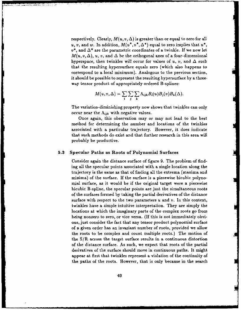
respectively. Clearly, M(u, v, A) is greater than or equal to zero for allu, v, and w. In addition, M(u*, v*, A*) equal to zero implies that u*,v*, and A* are the parametric coordinates of a twinkle. If we now letM(u, v, A), u, v, and A be the orthogonal axes of a four-dimensionalhyperspace, then twinkles will occur for values of u, v, and A suchthat the resulting hypersurface equals zero (which also happens tocorrespond to a local minimum). Analogous to the previous section,it should be possible to represent the resulting hypersurface by a three-way tensor product of appropriately ordered B-splines:

M(u,v,A) = Zi ,AijkkB(u)Bj(v)Bk(A).

The variation-diminishing property now shows that twinkles can onlyoccur near the Ai3k with negative values.

Once again, this observation may or may not lead to the bestmethod for determining the number and locations of the twinklesassociated with a particular trajectory. However, it does indicatethat such methods do exist and that further research in this area willprobably be productive.

5.3 Specular Paths as Roots of Polynomial Surfaces

Consider again the distance surface of figure 9. The problem of find-ing all the specular points associated with a single location along thetrajectory is the same as that of finding all the extrema (maxima andminima) of the surface. If the surface is a piecewise bicubic polyno-mial surface, as it would be if the original target were a piecewisebicubic B-spline, the specular points are just the simultaneous rootsof the surfaces formed by taking the partial derivatives of the distancesurface with respect to the two parameters u and v. In this context,twinkles have a simple intuitive interpretation. They are simply thelocations at which the imaginary parts of the complex roots go frombeing nonzero to zero, or vice versa. (If this is not immediately obvi-ous, just consider the fact that any tensor product polynomial surfaceof a given order has an invariant number of roots, provided we allowthe roots to be complex and count multiple roots.) The motion ofthe S/R across the target surface results in a continuous distortionof the distance surface. As such, we expect that roots of the partialderivatives of the surface should move in continuous paths. It mightappear at first that twinkles represent a violation of the continuity ofthe paths of the roots. However, that is only because in the search

40

for specular points, we were only interested in the roots with zeroimaginary part. Note that the requirement that specular points mustbe annihilated or created in pairs can be seen in this context as thefact that the roots which have nonzero imaginary parts must occur incomplex conjugate pairs.

Consider two methods for tracking specular points by searching forcomplex values of the u and v (call them ii and Z) parameters whichare extrema of the distance surface. The first is a brute-force method.If we think of each of the polynomial B-spline patches as being definedover the entire imaginary plane, then each patch will contain the samenumber of extrema (of course some of the extrema may be repeated).It should be possible to find all these complex extrema for a singletrajectory location and for each patch, then track the motion of thesecomplex points as the S/R moves along the trajectory. Those extremawhich have zero imaginary parts will be given the distinction of beingspecular points. Unfortunately, if the surface consists of thousands ofpolynomial patches, then even more thousands of complex extremawill have to be tracked for all positions along the trajectory to assurethe invariance in the number of extrema.

For a second method, suppose that the polynomial patches werelinked together so that not only the composite surface is smooth inthe sense we have been considering, but also the complex extremaof the surface are continuous across patches. With such a surface,it would only be necessary to find all the complex extrema with real

parts in the range for which we consider the patch to describe thesurface: i.e., the real parts of ii and i restricted to [0,11. Then asthe S/R moves along the trajectory, the only way that an extremumcould enter a new patch is if it leaves a neighboring patch (ignoring

for the moment the edges of the composite surface). If the compositesurface is closed, finding all the extrema with real parts in [0,1] willresult in finding an invariant set of complex extrema which is muchreduced from that of the previous brute-force method.

This method has the potential to be extremely powerful and effi-cient. Once all the complex extrema are found for any location, they

may be tracked to the beginning of any desired trajectory and thentracked along the desired trajectory. Note that it would be trivial toinclude arbitrary nonlinear trajectories. Note also that because theinvariant number of extrema need only be determined once for anygiven target, the methods used to find the extrema can be extremelythorough.

It should be noted that the search for complex roots can be con-

41

siderably more difficult than the search for strictly real roots. Onepotentially useful method for finding the complex roots of a B-splinepatch would be to find all the roots for a particular patch (with ii andi extended to the entire imaginary plane) chosen to simplify the prob-lem. Once all these roots are found, the B-spline coefficients could bemodified to the desired B-spline patch while the complex roots aretracked. This method would assure that all the complex roots arefound. Since neighboring patches tend to have similar coefficients,it should be natural and efficient to continue to deform patches intoneighboring patches while tracking the effect on the roots.

Unfortunately, cubic B-spline surfaces as used in this report do notprovide continuity of the complex roots across patches. One wouldhope that just as raising the order of the spline allows for additionalderivative continuity, perhaps the additional freedom of raising thespline order by one could be used to ensure continuity of the complexroots. Because of the very powerful potential of this method, therequirements for complex root continuity of the B-spline compositesurface should be investigated.

5.4 Twinkle Search Through Recursive Subdivision

It was pointed out in section 5.2 that if a portion of the surface issuch that its maximum and minimum principal radii of curvature bothpoint toward the interior of the surface, then no twinkles can exist onthat portion of the surface for any trajectory. Consider a generaliza-tion of this technique. Each point on a patch of the B-spline quilthas associated with it two principal radii of curvature (the maximumand minimum radii of curvature). Suppose the maximum and min-imum values of the two principal radii of curvature were known forthe entire patch. If we add to the two maxima an amount to accountfor the finite extent of the patch, and subtract from the minima thesame amount, the four resulting radii will provide two bounding vol-umes, one of which must be intersected by the trajectory if a twinkleis to occur on that patch; i.e., each principal radius of curvature willhave associated with it a range guaranteed to include its maximumand minimum values over the entire patch. If the trajectory does notpass through either of these two ranges, then the patch cannot con-tain a twinkle. Now consider what happens if the original patch issubdivided into four subpatches. The maximum and minimum val-ues of the two principal radii of curvature will become closer to thesame on each subpatch, decreasing the volume of space which must

42

be intersected by the trajectory for any of the subpatches to containa twinkle (the extent of the patch will decrease as well). In the limitas the patch is recursively subdivided, two concentric spheres will beformed, one of which the trajectory must intersect in order for thesubpatch to contain a twinkle.

The above method can be turned into a recursive subdivision tech-nique for finding twinkles by adding the requirement that a twinklemust also be a specular point. Using the normal at the center of apatch along with the maximum curvature for the patch, we can cal-culate a "normal cone" which includes all possible surface normalsfor the patch. As the patch is subdivided, each cone will becomesmaller in extent until, in the limit, the cone becomes a line. Twin-

kk will be assumed to exist only on those subpatches for which thetrajectory, normal cone, and space between appropriate concentriccurvature spheres all intersect. The subdivision can be carried out

until limited by the precision of the computer, at which time theremaining candidate subpatches may be considered the locations oftwinkles. Except for twinkles that lie so close together that the dif-ference in their positions cannot be distinguished with the precisionof the computer, the recursive subdivision technique should result in

finding all the twinkles for a given trajectory. It should be clear to thereader that the normal cone described above could also be used byitself to define a recursive subdivision test for initial specular points.

It should be possible to simplify the search for the maxima andminima of the two principal curvatures on each subpatch by first find-ing all stationary points of the principal curvatures for each originalpatch. The extrema of the principal curvatures on all subpatcheswould either have to be the extrema of the parent patch or lie alongthe edge of the subpatch, greatly simplifying the search for the maxi-mum and minimum curvatures of each subpatch. Note that the searchfor the curvature extrema on the original patches would only have tobe carried out once for the model since curvature extrema are indepen-dent of the chosen trajectory. It may even be possible to find efficientbounds on the maximum and minimum principal curvatures more di-rectly from the original data points by exploiting the properties of theB-spline surface.

5.5 Inclusion of Surface Discontinuities

The surfaces of most targets of interest are not everywhere second-order continuous. This is particularly obvious in manmade targets

43

which generally have an abundance of corners and edges. While itmay be possible to model edges and corners as second-order continu-ous surfaces containing locations of very small radius of curvature, inmany cases the modeling effort will be made much easier if the con-straint of second-order continuity everywhere is reduced; that is, ifthe surface is everywhere second-order continuous except along edgesor corners.

At first glance, it might appear that the use of twinkles to reducethe computational time required to simulate the return from complextargets would be of little use when the surface contains discontinuitiesof either its first or second derivatives; in such a situation, it wouldbe possible for specular paths to begin and end at places other thantwinkles. Fortunately, it is easy to see that for all the target surfacewhich is second-order continuous, specular paths can still only be cre-ated or destroyed at twinkles. Therefore, once the twinkles and initialspecular points are found, the specular paths can still be tracked, aslong as for each new trajectory location all the discontinuities are alsochecked. If the surface discontinuities occur at isolated points (cor-ners) or along curves (edges), the additional search required by theinclusion of discontinuities will be reduced in order. If in addition thediscontinuities are restricted to lie on parametric curves running or-thogonal to either of the two surface parameters, the problem becomesparticularly simple. For example, the surface normal along one edgeof a B-spline patch is a function of only one parameter (with properchoice of axes, the other parameter will be fixed at zero). Thus if adiscontinuity lies along the edge of a B-spline patch, it should be astraightforward procedure to find any intersections between the sur-face normal along the edge and the trajectory. The intersections couldbe thought of as "pseudo-twinkles" since they represent additionalpoints on the surface at which a specular path may begin or end. If itis necessary to include discontinuities along parametric curves whichare not orthogonal to either of the two surface parameters, the algebrabecomes somewhat more unwieldy. However, it should still be a fairlystraightforward task to find the pseudo-twinkles along the curves foran entire trajectory. Thus the inclusion of curvature, slope, or evenposition discontinuities in the target surface is another topic whoseinvestigation should prove fruitful.

44

5.6 Multiple Bodies and Shadowing

Backscatter simulation algorithms based on twinkles are just as ap-plicable to multibody targets as they are to single-body targets. Evenfor multiple bounces, the question of whether the bounces occur onseparate bodies or not never enters into the problem. The problemwith finding the return from a target made up of separate bodies isthat the effect of shadowing becomes more important; i.e., it is morelikely that the ray being considered will have passed through part ofthe target. Recall that the stationary condition for multiple-bouncereturn shown earlier (which includes the single-bounce case) does notrequire such an unobstructed path.

Questions related to shadowing are almost always handled by someform of ray tracing. However, the computational savings due to theuse of twinkles would be totally eliminated if it were still necessaryto ray trace the entire scene just to handle the shadowing. Thosespecular points which have been found by ignoring potential shadow-ing we refer to as "potential specular points." Clearly, the problemof determining whether or not a potential specular point is an actualspecular point is greatly simplified by knowledge of its position. Atmost it will be necessary to check only the paths associated with eachspecular point for intersections with the target surface at each tra-jectory location to determine the actual "visibility" of the return. Itmay even be possible to exploit the continuity of the target surfaceto reduce the computational time required to search for shadowingstructures. For example, if the path connecting a multiple-bouncereturn is to go from being unshadowed to shadowed, some portionof the path must become osculatory with the target surface at somepoint. And of course the same must hold for a multiple bounce comingout of shadow. Once the potential specular paths have been deter-mined (ignoring potential shadowing), it may be possible to exploitthis shadowing constraint to rapidly determine which portions of thepaths should be considered actual specular paths for calculating theexpected return.

5.7 Experimental Validation and Comparison

The ultimate goal of this study is to develop a useful radar backscat-ter modeling technique for such targets as tanks, aircraft, and ships.Clearly then an experiment of interest would be to create a splinemodel which closely resembles the surface of a target of interest, ex-perimentally determine the backscatter signatures of the actual target

45

for many trajectories, and compare the results with those calculatedfrom the spline surface using a geometric optics approach. Whilesuch experiments will eventually determine the bottom-line effective-ness of the modeling approach, an intermediate set of experimentsusing a target developed to test specific assumptions of the modelingmethod should also prove to be informative.

Generally speaking, the use of a geometric optics assumption forthe return from complex targets is subject to two broad categories oferror. The first type of error is due to the surface description not ad-equately resembling the actual target surface of interest. The secondcategory of error is due to the geometric optics assumptions them-selves (i.e., everything else). For a target such as a tank, there arelikely to be a number of items which do not fit the geometric assump-tions well. Sharp edges, varying surface material properties, or justplain dirt are only a few examples. A useful experiment thereforewould be to construct a complex surface which satisfies the geometricoptics assumptions to a high degree for an available radar frequency.The surface should then be accurately modeled by B-splines and theactual and simulated returns compared. Comparisons of signaturesusing various frequencies and trajectories should lead to greater in-sight into the overall modeling problem as well as into the limits ofthe geometric optics approach.

Once a geometric optics model is chosen to simulate the returnfrom complex targets, the method used to find the specular pointsmakes no difference in the calculation of the return (provided eachmethod finds all the specular points for each location of the trajec-tory). However, the ability to rapidly find all the specular points as afunction of the trajectory location does give the ability to conduct amore extensive validation of the model. Such an extensive validationof the model should be performed for a complex but highly controlledtarget for which the geometric optics assumptions are valid, as wellas for actual targets of interest.

46

6. Summary

Use of the geometric optics approach to simulate the radar backscatterfrom composite targets can be efficient and informative. The valid-ity of the approach depends on a number of factors, including thetarget surface characteristics and the wavelength of the propagatedsignal. The use of B-splines to describe complex targets for use inthe geometric optics model is an obvious extension of previous meth-ods. Unfortunately, the increased complexity of the model means anincreased search time for a generally unknown number of specularpoints. Since it is expected that the specular points must be foundfor thousands of locations along each trajectory, ordinary techniqueswhich search the entire surface for specular points, at each location onthe trajectory, are generally too computer intensive to be practical.

Over 25 years ago, Longuet-Higgins [8] pointed out the continu-ity of specular paths on smooth surfaces and showed the conditionsfor which a specular path may become discontinuous. It has beenshown in this paper that the locations of specular path discontinu-ities (known as twinkles) may be predicted for an entire trajectory.Once the locations of all the twinkles associated with a particular tra-jectory are known, it is only necessary to track the motion of specularpoints as a function of the trajectory location, assured that creationsand annihilations of specular paths will only occur at the twinkles. Itwas shown that the method extends to multiple bounces of any order.

The actual algorithms currently used to find twinkles and initialspecular points are implementations of simple local gradient tech-niques, which offer no assurance of convergence to all the desiredpoints. The shortcomings of these techniques were discussed and sug-gestions were made for techniques to increase the robustness of thealgorithms. In addition, the problems of surface discontinuities andshadowing were briefly discussed, with the conclusion that they maybe included in the model without negating the savings incurred by us-ing twinkles. The inclusion of surface discontinuities and shadowingare two more suggested topics of further research.

Consider the problem of simulating the backscatter from a targetrepresented by the equivalent of 10,000 B-spline surface patches for1000 locations along a specified trajectory. The author anticipatesthat pursuit of the research suggested in this report will result inalgorithms to find the backscatter signatures from such encounters in amatter of minutes, on a reasonably high-powered computer. It shouldbe possible with such a model to capture the significant features of

47

most complex targets of interest. Such a model would obviously findimportant applications in many current as well as anticipated projectsusing high-frequency radar as a source of information.

References

[1] John F. Dammann, Air Target Models for Fuzing Simulations,Harry Diamond Laboratories, HDL-TR-1960 (September 1982).

[21 Carl de Boor, A Practical Guide to Splines, Springer-Verlag, NewYork (1978).

[31 William J. Gordon and Richard F. Riesenfeld, B-Spline Curvesand Surfaces, Proc., Computer Aided Geometric Design Confer-ence, University of Utah, Salt Lake City (18-21 March 1974).

[4] M. G. Cox, The Numerical Evaluation of B-Splines, J. Inst.Math. Its Appl. 10 (1972), 134-149.

[5] Donald E. Amos, Computation with Splines and B-Splines, San-dia National Laboratory, SAND78-1968 (March 1979).

[6] David G. Luenberger, Linear and Nonlinear Programming,Addison-Wesley, Reading, MA (1984).

[7] Elaine Cohen, Tom Lyche, and Richard Riesenfeld, Discrete B-Splines and Subdivision Techniques in Computer-Aided Geomet-ric Design and Computer Graphics, Computer Graphics and Im-age Processing 14 (1980), 87-111.

[8] M. S. Longuet-Higgins, Reflection and Refraction at a RandomMoving Surface. I. Pattern and Paths of Specular Points, J. Opt.Soc. Am. 50 (1960), 838.

[91 Ivor D. Faux and Michael J. Pratt, Computational Geometry forDesign and Manufacture, Ellis Horwood, New York, NY (1981).

48

Appendix A. Newton Step for the Location of a Specular Pointon a B-Spline Surface

We are interested in solving the matrix equation( F1 OF1F2 F2 S 2 -F

where 2

F1 Fl(u,v,A) = OI1G(u, v,A)1Ott

F2 F2(u,v,A)= 0 IIG(uv,A)112

OIf we let the z, y, z coordinates of figure 2 in the body of the report bereplaced by X 1 ,X 2 ,X 3 , respectively, the equation for IIG(u,v, A)112

becomes3

IIG(u,v,/A)112 = Z[A(X' - X') + X' -R(u, V)]2= 1

where R,. is the X' component of the surface R(u, v). Then,

3 ~OR.-i(u, v) 'F(u,,,A) = -2_ 1 [A(Xi - Xi) + X' - R.,(u,v)] ,F(u,V,A) = -2 [a(X-X) + X' - R,(u, v)]

E2 lt2 1 1Ov

o% i=1l

_________0 2R.(u,,,)OF(u,v,,A) = -2 3 [A(Xi - Xi) + Xi - R, (0,,,)] uv

Oui i=1"OR. (u, v) I 2Ou

OF2(u, v, A) 2 X+ R2,(u, v)

Ov 0 2 AX i -Ru vOV i=1

'u

O Ou

19

i~ ~ ~ ~ ~ ~ ~ ~~O~ (um -,llliil v)lil~ ORiiiNH l.. (u v)

Appendix A

Let Aij be the vector coefficients .f a single B-spline patch and denoteits z, y, or z component by A . Then for the 1, mth patch of thebicubic B-spline surface being considered,

4 4

R1.,m&(u, v) E Z Z Bi(u)A +,j+M Bj(v),=1 j~l

where Bi(z) for i=1, 2, 3, and 4 were given in section 1.3 and u,v E[0, 1]. Thus, for any particular patch and trajectory, given u, v, andA, the Newton step [S1,S2] toward a specular point is given by

(OF, OF 1

-1

&U Ov

If u, v, and A are not the coordinates of a twinkle, then the inversein the previous equation is guaranteed to exist.

50

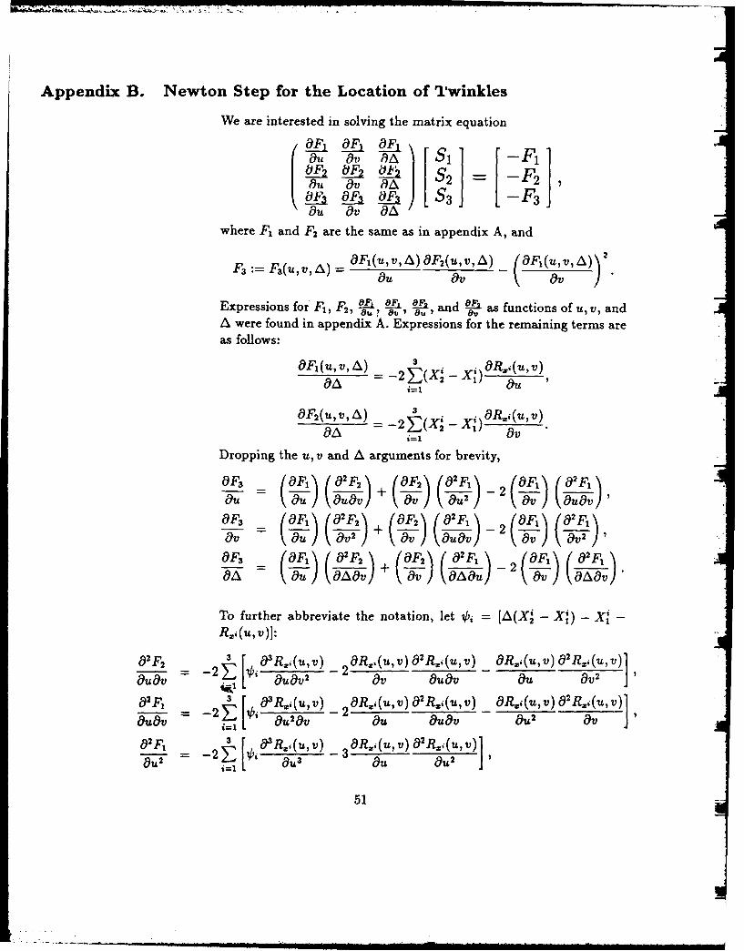
Appendix B. Newton Step for the Location of Twinkles

We are interested in solving the matrix equationOF O OF 0 FFOF, fa A S -F1

oLF $ 2 = [ -F]Oi(911, 19V (9A SOF 3 -F

19u O#v OAwhere F and F2 are the same as in appendix A, and

F3 F(~,)=OF, (u, v, A) OF2 (u, v, 0)F1uv7AF3 := F3(u, v,A) = f(u)OfUva _O V \a1u !OV

Expressions for F1 , F2, I, L 9 , and -I as functions of u, v, andA were found in appendix A. Expressions for the remaining terms areas follows:

OF,(u, v, A) = - Xi)ORi,(u, v)i=IiO9A -2 2 1 Ou

OF2 (u, v, = -23(x - x)9R.i

19A #i=9V

Dropping the u, v and A arguments for brevity,

OF (OF 1 ( OF 2 ( , (F2 OF 1 2 OF, (,2, )F-

OF3 (OF2 F (OF [(9F 1\

F#)k F2 ) + #9)O-k #972)

oF-3 = (-O-\ -#9F )+kF #-9-F1 \a- -2\ OF1 02F1 /

M u OA9v #9V O9u) (Wv )(AOv)To further abbreviate the notation, let , = [A(X' - X') - X'R~i(u, v)]:

O 2 F 2 OR3R2 (uv) 2 ORfi(uv)8 2 Ri.(uv) _ OR 3 (u,v) 2 ) R (u,v)1=UO -2 ' OuOv2 2 Ov OUOv OU OV2

a219 3 83 R, (u,"v) 2 ORi (u, v) 2 R ) (u, v OR.(u,,v)o 2R.(u,v).5u~qv -2~ OU2OV - OU OuOV &2 OV 3a2F F,3[iO 3R21i(u,v) 3 ORi (u, v) 192 R~iu, v)1

OL2 OU3 -3 O9u OU2

t=1

51

Appendix B

a2F2 2 [,i 3R ..(u, v) 3 OR~ (u, v) 02 R ,(u,v)

,2 F2 3 -9 49?) &v2)

2 - 2(X2'- Xl) O 2 uv

,92F, 3 (92 Riu,v)2 E2(X'-X) 8u

OAO9u l2 1 U

a X 1 _~ (2 4u, v)

52

. . .. I !1 1 I 'l I -., _ , .... .

Appendix C. Taylor Coefficients at a Twinkle in the Rotated Frame

At a twinkle, the Taylor coefficients a~jA are given by

=0+j+k JIG(u,v, A)I2aijk = OUiOVj OA k .,t,

where utw, vtw, and Atu, are the coordinates of the twinkle. We areinterested in the Taylor coefficients a30 0, aoll, a0 2o, a210 , and a10 1 inthe u', v', A' coordinate system, where

u = u'cos0 - v'sinO + ut.

v = u' sin 0 - v'cos 0 + vtw.

Let At. be the scalar components of the vector coefficients of asingle B-spline patch, with Ak representing the z, y, or z coordinatesas k = 1, 2, or 3 respectively. Then,

3. 4 4 ,2

IIG(u,v, A)112 - [,(a) _ ZZ B(u)A 3 B(V)

where lbk was defined in appendix B,

0[1ch-2 _ 1 [0 4 4 [OB=(u-2 _ k E Bj(u)AkBj(V) E u AliBi(v)

,9 'k=1 i,j=l i-j=l

+ Bj(u)A ' 0B(v)

02 JIG12 -2 3 (Xkf k) [0Bj(u ) Ak Bj + Bj(\Ak- OB,(v)1OU'0A E 2~I 1X'X C Oi' , 0()9LJIuJ ,

02 1311 14 0 1 uJIG2 I -h _ B(u)A ,B1 (v [,02 U )A B (v)

k=1 I j i,7=

+2 O-u) A- O-(v) + Bu(u)A9

Ou t13au

G)2- E +(u)A, ) )A:B(v)

O~U'3 - - k~~~i~J _ )u3 V BAB3 A1 3 (

53

Appendix C

&9B(U) 8.Bi(v) 38 Bj(u)A 9'Bj(v) +Bj(uA&- a3B3 (v)1

+3 A & '3 -u + 3-Au' OUa'2 + \t) 3 aL 3 3

-3 B[M(u) A ,B,(v) + Bj(u)A -OB#) 4

ra2Bl( B(u) Ak. aB3(v)+2 - A -5 + Bj(u)A - j f(vOu'2 AS ()+ u Eh.' u'2

The expressions for B2 4VI and 2IIGff can be obtained directly from

the expressions for 2W and 21 epectivelybyrpaiguwt

v' throughout:

03 JI 11 3 4~u~ 4~ 92 -B(u) At' OBjv)')'2V 2k ju) 3,B (v) 19U'2 1 V'I

+ Ou-BOu) A -B1 (v) + 2 - (v B) +2 B( A-Oj(V

kO3Bi(v)ju) a2 B3 (v) 1I 8B1 (u) k Bjv

+Bi(u)A1 3 A +2

~~~~ 19Bv 13FO~~k8 3 v

~I ~41AO#) + [ 0 2 B(U) AB(v) + 2 1(uA aB 3 v011(u) Ak -9Bbu v2ou ll1u

qv "5 &

A - '-jv) 2B(-) A - 8t' ()A - d? oLB Frt tha 'qV Oue= cosO, -s

+'B~u OkAtu) [oulOV, S3 out

Itrembains sotrie is aiu ata eivtvs'ij- n

Ou%& Ou' OV O' O u

co adfuter ht l hgerode eivtve54 n

Appendix C

If the conjecture holds for the kth partial derivative, then

0 O'B'(u) _OkB,(u) [nIkI[82_1 + B() [On [,,n k

OU' iOu'k - OUkk'U OU' 2 j 0uk+1 19U 19Uj[ ,i- "9+lB.(u) [ Ou I k+'

Similarly,ak Bt(v) _OkBi(v) [Ov 1k

OkBi(u) _OkBi(u) [au 1 k

49vk t O0uk [O9V'J

OkB 1(V) _k 13,(V) [O k

'k O-v-k L[u' jAnd further, it can be shown that

ak+LBi(u) _ "+B(u) [O i 1 Jk N I

6?U 1k&vJ Oquk+L [ ~J I Vi

adOB(U') (COS 9)k( sin8)Ou'k~v'L Ok+1 n [OJ

&+'Bi~v) &+B(v) rO ei

&+l (sin O)k (cos 0)1,

55k~

DISTRIBUTION

ADMINISTRATOR COMMANDERDEFENSE TECHNICAL INFORMATION CENTER US ARMY MISSILE COMMAND (Cont'd)ATTN DTIC-DDA (12 COPIES) ATTN DRCPM-ROL, ROLANDCAMERON STATION, BUILDING 5 ATTN DRSMI-T, TARGETS MANAGEMENT OFFICEALEXANDRIA, VA 22304-6145 REDSTONE ARSENAL, AL 35809

COMMANDER DIRECTORUS ARMY ARMAMENT, MUNITIONS, & US ARMY MISSILE LABORATORYCHEMICAL COMMAND USAMICOM

ATTN DRSMC-LEP-L, TECHNICAL LIBRARY ATTN DRSMI-RD, SYS SIMULATION & DEV DIRATTN DRSMC-ASF, FUZE & MUNITIONS REDSTONE ARSENAL, AL 35809

SUPPORT DIVROCK ISLAND, IL 61299 ASSISTANT SECRETARY OF THE NAVY

RESEARCH, ENGINEERING, & SYSTEMSDEPT OF THE AIR FORCE, HQ DEPT OF THE NAVY6585TH TEST GROUP (AFSC) WASHINGTON, DC 20350RADAR TARGET SCATTER FACILITYATTN LT COL RONALD L. KERCHER, CHIEF US ARMY LABORATORY COMMANDHOLLOMAN AFB, NM 88330 ATTN TECHNICAL DIRECTOR, AMSLC-TD

ENGINEERING SOCIETIES LIBRARY INSTALLATION SUPPORT ACTIVITYATTN ACQUISITIONS DEPARTMENT ATTN LEGAL OFFICE, SLCIS-CC345 EAST 47TH STREETNEW YORK, NY 10017 USAISC

ATTN RECORD COPY, ASNC-LAB-TSDIRECTOR ATTN TECHNICAL REPORTS BRANCH, ASNC-LAB-TRDEFENSE ADVANCED RESEARCH (2 COPIES)

PROJECTS AGENCYARCHITECT BLDG HARRY DIAMOND LABORATORIESATTN TARGET ACQUISITION ATTN D/DIVISION DIRECTORS

& ENGAGEMENT DIV ATTN LIBRARY, SLCHD-TL (3 COPIES)1400 WILSON BLVD ATTN LIBRARY, SLCHD-TL (WOODBRIDGE)ARLINGTON, VA 22209 ATTN CHIEF, SLCHD-NW-E

ATTN CHIEF, SLCHD-NW-EHOFF OF THE ASSISTANT SECRETARY ATTN CHIEF, SLCHD-NW-EP

OF THE ARMY (RDA) ATTN CHIEF, SLCHD-NW-ESATTN DEP FOR COMMUNICATIONS ATTN CHIEF, SLCHD-NW-R

& TARGET ACQUISITION ATTN CHIEF, SLCHD-NW-CSWASHINGTON, DC 20310-0103 ATTN CHIEF, SLCHD-NW-RP

ATTN CHIEF, SLCHD-NW-RSCOMMANDING OFFICER ATTN CHIEF, SLCHD-NW-TNUS ARMY FOREIGN SCIENCE ATTN CHIEF, SLCHD-NW-TS

& TECHNOLOGY CENTER ATTN CHIEF, SLCHD-NW-PFEDERAL OFFICE BLDG ATTN D. R. COOK, SLCHD-ST-AAATTN AMXST-SC, SCIENCES DIV ATTN J. BRUNO, SLCHD-ST-AP220 7TH STREET, NE ATTN H. C. LISINSKI, SLCHD-ST-SA (10 COPIES)CHARLOTTESVILLE, VA 22901 ATTN J. W. MILLER, SLCHD-TA-SS

ATTN R. D. CHRISTOPHERSON, SLCHD-TA-SSCOMMANDER ATTN K. REINIG, SLCHD-ST-SA (30 COPIES)US ARMY MISSILE COMMANDATTN DRCPM-CF, CHAPARRAL/FAAR

57