Embed Size (px)
Citation preview

RAPIDLY SHEARED COMPRESSIBLE TURBULENCE:
CHARACTERIZATION OF DIFFERENT PRESSURE REGIMES AND EFFECT
OF THERMODYNAMIC FLUCTUATIONS
A Thesis
by
REBECCA LYNNE BERTSCH
Submitted to the Office of Graduate Studies ofTexas A&M University
in partial fulfillment of the requirements for the degree of
MASTER OF SCIENCE
August 2010
Major Subject: Aerospace Engineering

RAPIDLY SHEARED COMPRESSIBLE TURBULENCE:
CHARACTERIZATION OF DIFFERENT PRESSURE REGIMES AND EFFECT
OF THERMODYNAMIC FLUCTUATIONS
A Thesis
by
REBECCA LYNNE BERTSCH
Submitted to the Office of Graduate Studies ofTexas A&M University
in partial fulfillment of the requirements for the degree of
MASTER OF SCIENCE
Approved by:
Chair of Committee, Sharath GirimajiCommittee Members, Jacques Richard
Prabir Daripa
Head of Department, Dimitris Lagoudas
August 2010
Major Subject: Aerospace Engineering

iii
ABSTRACT
Rapidly Sheared Compressible Turbulence:
Characterization of Different Pressure Regimes and Effect of Thermodynamic
Fluctuations. (August 2010)
Rebecca Lynne Bertsch, B.A., Colorado College
Chair of Advisory Committee: Dr. Sharath Girimaji
Rapid distortion theory (RDT) is applied to compressible ideal-gas turbulence
subjected to homogeneous shear flow. The study examines the linear or rapid pro-
cesses present in turbulence evolution. Specific areas of investigation include:(i) char-
acterization of the multi-stage flow behavior,(ii) changing role of pressure in the three-
regime evolution and (iii) influence of thermodynamic fluctuations on the different
regimes. Preliminary investigations utilizing the more accurate Favre-averaged RDT
approach show promise however, this approach requires careful validation and testing.
In this study the Favre-averaged RDT approach is validated against Direct Nu-
merical Simulation (DNS) and Reynolds-averaged RDT results. The three-stage
growth of the flow field statistics is first confirmed. The three regime evolution of
turbulence is then examined in three different timescales and the physics associated
with each regime is discussed in depth. The changing role of pressure in compressible
turbulence evolution shows three distinct stages. The physics of each stage is clearly
explained. Next, the influence of initial velocity and thermodynamic fluctuations on
the flow field are investigated. The evolution of turbulence is shown to be strongly
dependent on the initial gradient Mach number and initial temperature fluctuations
which tend to delay the onset of the second regime of evolution. The initial tur-
bulent Mach number, which quantifies velocity fluctuations in the flow, influences
turbulence evolution only weakly. Comparison of Reynolds-averaged RDT against

iv
Favre-averaged RDT for simulations of nonzero initial flow field fluctuations shows
the higher fidelity of the latter approach.

v
To my family who have always urged me to do my best.

vi
ACKNOWLEDGMENTS
I would like to take this opportunity to thank everyone who aided me during
my graduate career and helped me complete my Master’s thesis. First of all, I would
like to thank my graduate advisor, Dr. Sharath Girimaji, for helping me develop
the necessary research skills to be successful. His unique teaching ability has aided
me in understanding the fundamental concepts of fluid turbulence. I would like to
thank Dr. Jacques Richard and Dr. Prabir Daripa for their participation on my
committee and giving relevant feedback in the thesis writing process. My research
with Dr. Richard in summer 2006 was my first experience in turbulence and was a
major influence on my graduate career. The coursework I took with Dr. Daripa was
invaluable to my research. I would like to thank the staff of the Aerospace Engineering
Department for all their help. Special thanks to Karen Knabe for her expertise in the
Thesis/Dissertation paperwork deadlines.
I would like to personally thank Sawan Suman for acting as a mentor throughout
my graduate career. Sawan’s knowledge of my field of research greatly influenced my
understanding of my work . Even after completion of his dissertation he continued to
respond to my inquisitive emails and verify my research results. I also appreciate the
support and assistance the rest of my research group has given me in the past three
years. Our weekly turbulence discussions have given me insight into other areas of
research.
I must acknowledge my family and friends back home in Colorado who continue
to support me even though they wish I weren’t so far away.
And finally, to all my amazing friends in the department, thanks for your support,
discussions and laughter.
This work was supported by NASA MURI research grant and the Hypersonics

vii
Center at Texas A & M University.
viii
TABLE OF CONTENTS
CHAPTER Page
I INTRODUCTION . . . . . . . . . . . . . . . . . . . . . . . . . . 1
A. Motivation . . . . . . . . . . . . . . . . . . . . . . . . . . . 1
B. Rapid Distortion Theory: A Literature Review . . . . . . . 4
C. Research Goals . . . . . . . . . . . . . . . . . . . . . . . . 5
D. Thesis Outline . . . . . . . . . . . . . . . . . . . . . . . . . 5
II RAPID DISTORTION THEORY FOR COMPRESSIBLE FLOWS 7
A. Reynolds Averaged Statistics . . . . . . . . . . . . . . . . . 7
1. Methodology . . . . . . . . . . . . . . . . . . . . . . . 7
a. Homogeneity Assumption . . . . . . . . . . . . . 10
b. Linearization . . . . . . . . . . . . . . . . . . . . 11
c. Spectral Transformation . . . . . . . . . . . . . . 12
d. Particle Representation Method . . . . . . . . . . 13
B. Favre-Averaged Statistics . . . . . . . . . . . . . . . . . . . 15
1. Methodology . . . . . . . . . . . . . . . . . . . . . . . 15
a. Homogeneity Assumption . . . . . . . . . . . . . 18
b. Linearization . . . . . . . . . . . . . . . . . . . . 19
c. Spectral Transformation . . . . . . . . . . . . . . 20
d. Particle Representation Method . . . . . . . . . . 20
C. Numerical Implementation and Validation . . . . . . . . . 23
1. Numerical Implementation . . . . . . . . . . . . . . . 23
2. R-RDT Validation . . . . . . . . . . . . . . . . . . . 24
3. F-RDT Validation . . . . . . . . . . . . . . . . . . . . 28
III CHARACTERIZATION OF THREE-STAGE BEHAVIOR . . . 30
A. Three-Stage Behavior in Different Timescales . . . . . . . . 31
1. Shear Time . . . . . . . . . . . . . . . . . . . . . . . . 32
2. Acoustic Time . . . . . . . . . . . . . . . . . . . . . . 32
3. Mixed Time . . . . . . . . . . . . . . . . . . . . . . . 33
4. Regimes of Evolution . . . . . . . . . . . . . . . . . . 34
B. Evolution of Gradient and Turbulent Mach Numbers . . . 34
C. Physics of Different Regimes . . . . . . . . . . . . . . . . . 36
1. Regime 1 . . . . . . . . . . . . . . . . . . . . . . . . . 40
ix
CHAPTER Page
2. Regime 2 . . . . . . . . . . . . . . . . . . . . . . . . . 44
3. Regime 3 . . . . . . . . . . . . . . . . . . . . . . . . . 48
IV POLYTROPIC COEFFICIENT . . . . . . . . . . . . . . . . . . 54
V EFFECT OF THERMODYNAMIC FLUCTUATIONS . . . . . 57
A. Kinetic Energy . . . . . . . . . . . . . . . . . . . . . . . . 57
1. Initial Temperature Fluctuation Intensity . . . . . . . 57
2. Initial Turbulent Mach Number . . . . . . . . . . . . . 58
B. Equi-Partition Function . . . . . . . . . . . . . . . . . . . 59
1. Initial Temperature Fluctuation Intensity . . . . . . . 60
2. Initial Turbulent Mach Number . . . . . . . . . . . . . 61
C. Influence on Transition Times . . . . . . . . . . . . . . . . 61
1. Regime 1-2 Transition Time . . . . . . . . . . . . . . . 62
2. Regime 2-3 Transition Time . . . . . . . . . . . . . . . 63
VI CONCLUSIONS . . . . . . . . . . . . . . . . . . . . . . . . . . . 67
A. F-RDT Validation . . . . . . . . . . . . . . . . . . . . . . . 67
B. Three timescales . . . . . . . . . . . . . . . . . . . . . . . 68
C. Three-Regime Evolution . . . . . . . . . . . . . . . . . . . 68
D. Role of Pressure in Three Regimes . . . . . . . . . . . . . . 69
E. Effect of Thermodynamic Fluctuations . . . . . . . . . . . 69
F. Transition Times . . . . . . . . . . . . . . . . . . . . . . . 69
REFERENCES . . . . . . . . . . . . . . . . . . . . . . . . . . . . . . . . . . . 71
VITA . . . . . . . . . . . . . . . . . . . . . . . . . . . . . . . . . . . . . . . . 74

x
LIST OF TABLES
TABLE Page
I Case Parameter Values . . . . . . . . . . . . . . . . . . . . . . . . . . 25
xi
LIST OF FIGURES
FIGURE Page
1 Schematic of various approaches for turbulence calculations. De-
creasing order of accuracy and computational effort from left to
right. . . . . . . . . . . . . . . . . . . . . . . . . . . . . . . . . . . . 2
2 Roadmap of steps required to apply different approaches to real-
istic scenarios. RDT provides second moment closure modeling
to obtain the 7-equation SMC. . . . . . . . . . . . . . . . . . . . . . 3
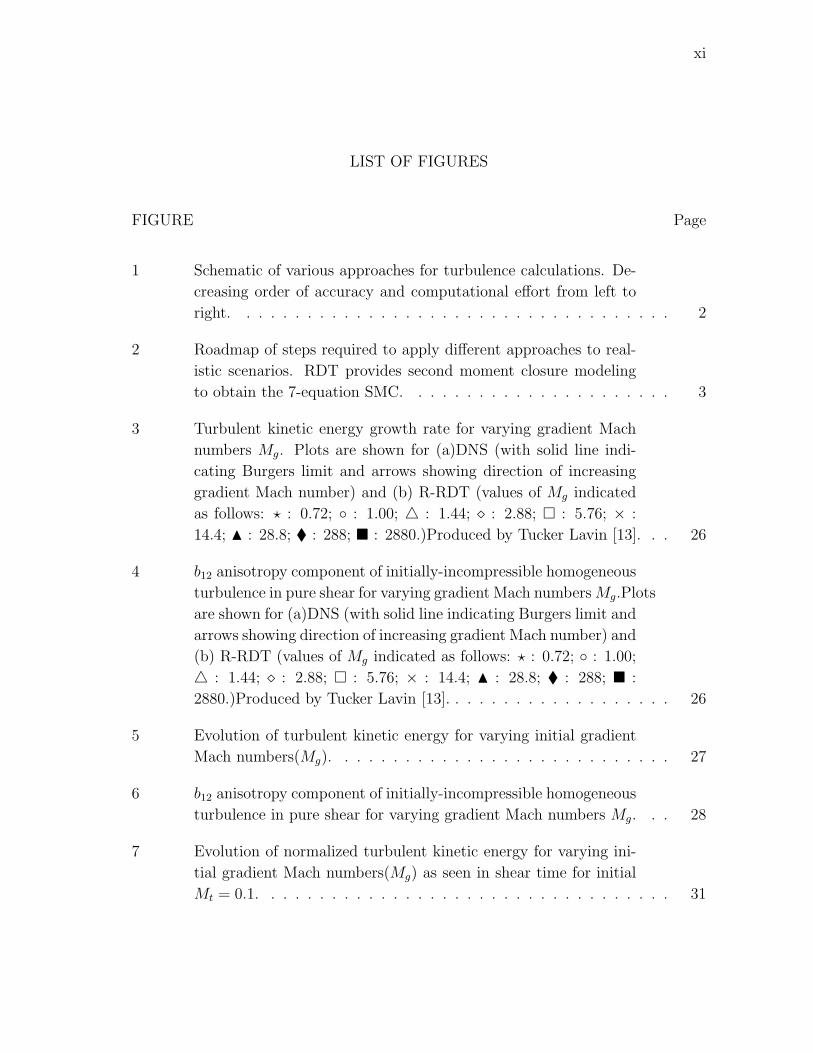
3 Turbulent kinetic energy growth rate for varying gradient Mach
numbers Mg. Plots are shown for (a)DNS (with solid line indi-
cating Burgers limit and arrows showing direction of increasing
gradient Mach number) and (b) R-RDT (values of Mg indicated
as follows: ? : 0.72; ◦ : 1.00; 4 : 1.44; � : 2.88; � : 5.76; × :
14.4; N : 28.8; � : 288; � : 2880.)Produced by Tucker Lavin [13]. . . 26
4 b12 anisotropy component of initially-incompressible homogeneous
turbulence in pure shear for varying gradient Mach numbersMg.Plots
are shown for (a)DNS (with solid line indicating Burgers limit and
arrows showing direction of increasing gradient Mach number) and
(b) R-RDT (values of Mg indicated as follows: ? : 0.72; ◦ : 1.00;
4 : 1.44; � : 2.88; � : 5.76; × : 14.4; N : 28.8; � : 288; � :
2880.)Produced by Tucker Lavin [13]. . . . . . . . . . . . . . . . . . . 26
5 Evolution of turbulent kinetic energy for varying initial gradient
Mach numbers(Mg). . . . . . . . . . . . . . . . . . . . . . . . . . . . 27
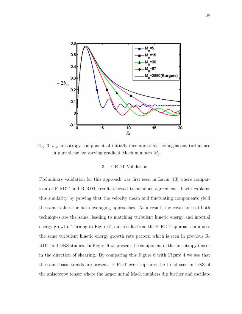
6 b12 anisotropy component of initially-incompressible homogeneous
turbulence in pure shear for varying gradient Mach numbers Mg. . . 28
7 Evolution of normalized turbulent kinetic energy for varying ini-
tial gradient Mach numbers(Mg) as seen in shear time for initial
Mt = 0.1. . . . . . . . . . . . . . . . . . . . . . . . . . . . . . . . . . 31

xii
FIGURE Page
8 Evolution of normalized turbulent kinetic energy for varying ini-
tial gradient Mach numbers(Mg) as seen in acoustic time for initial
Mt = 0.1. . . . . . . . . . . . . . . . . . . . . . . . . . . . . . . . . . 32
9 Evolution of normalized turbulent kinetic energy for varying ini-
tial gradient Mach numbers(Mg) as seen in mixed time for initial
Mt = 0.1. . . . . . . . . . . . . . . . . . . . . . . . . . . . . . . . . . 33
10 Evolution of gradient Mach number in shear time-scale. . . . . . . . 34
11 Evolution of gradient Mach number in acoustic time-scale. . . . . . . 35
12 Evolution of gradient Mach number in mixed time-scale. . . . . . . . 35
13 Evolution of turbulent Mach number in shear time-scale for zero
initial temperature fluctuations and an initial Mg = 5. . . . . . . . . 37
14 Evolution of turbulent Mach number in acoustic time-scale for
zero initial temperature fluctuations and an initial Mg = 5. . . . . . . 37
15 Evolution of turbulent Mach number in mixed time-scale for zero
initial temperature fluctuations and an initial Mg = 5. . . . . . . . . 38
16 Evolution of production and time rate of change of reynolds stresses
in shear time-scale for Mg = 5. . . . . . . . . . . . . . . . . . . . . . 39
17 Evolution of production and time rate of change of reynolds stresses
in acoustic time-scale for Mg = 5. . . . . . . . . . . . . . . . . . . . . 39
18 Evolution of production and time rate of change of reynolds stresses
in mixed time-scale for Mg = 5. . . . . . . . . . . . . . . . . . . . . . 40
19 Evolution of production and time rate of change of Reynolds
stresses in mixed time-scale during the first stage of evolution. . . . . 41
20 Evolution of fluctuating pressure moment in mixed time-scale dur-
ing the first stage of evolution. . . . . . . . . . . . . . . . . . . . . . 42
21 Evolution of dilatational kinetic energy in mixed time-scale during
the first stage of evolution. . . . . . . . . . . . . . . . . . . . . . . . . 43

xiii
FIGURE Page
22 Evolution of the increment in thermal energy in mixed time-scale
during the first stage of evolution. . . . . . . . . . . . . . . . . . . . 44
23 Evolution of production and time rate of change of Reynolds
stresses in mixed time-scale during the second stage of evolution. . . 45
24 Evolution of fluctuating pressure moment in mixed time-scale dur-
ing the second stage of evolution. . . . . . . . . . . . . . . . . . . . . 46
25 Evolution of dilatational kinetic energy in mixed time-scale during
the second stage of evolution. . . . . . . . . . . . . . . . . . . . . . . 47
26 Evolution of the increment in thermal energy in mixed time-scale
during the second stage of evolution. . . . . . . . . . . . . . . . . . . 47
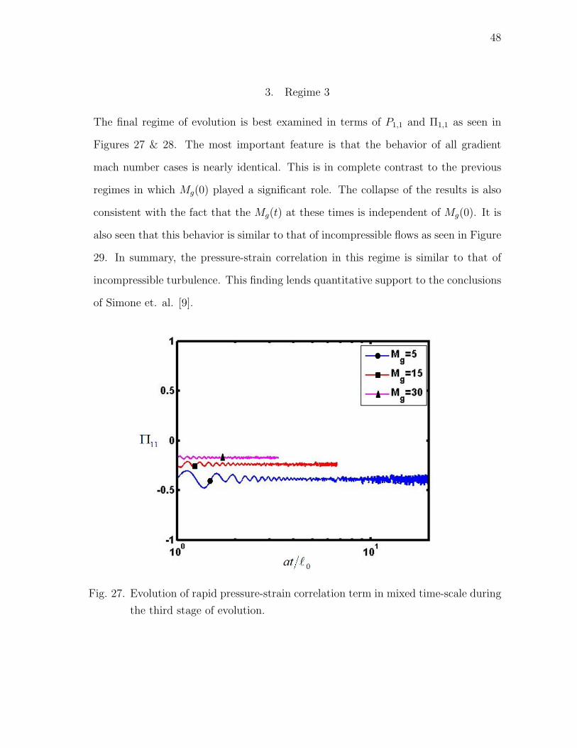
27 Evolution of rapid pressure-strain correlation term in mixed time-
scale during the third stage of evolution. . . . . . . . . . . . . . . . . 48
28 Evolution of the production term in mixed time-scale during the
third stage of evolution. . . . . . . . . . . . . . . . . . . . . . . . . . 49
29 Evolution of rapid pressure-strain correlation and production terms
in the incompressible limit, shown in mixed time-scale. . . . . . . . . 50
30 Evolution of Poisson pressure fluctuations in the acoustic time-scale. 52
31 Evolution of compressible pressure fluctuations in the acoustic
time-scale. . . . . . . . . . . . . . . . . . . . . . . . . . . . . . . . . . 52
32 Evolution of residial pressure fluctuations in the acoustic time-scale. . 53
33 Evolution of Averaged Polytropic coefficent for large initial tur-
bulent Mach numbers for Mg = 5 via R-RDT approach. . . . . . . . 55
34 Evolution of Averaged Polytropic coefficent for large initial tur-
bulent Mach numbers for Mg = 5 via F-RDT approach. . . . . . . . . 56
35 Evolution of Turbulent Kinetic Energy for different initial tem-
perature fluctuations for Mg(0) = 5 and Mt(0) = 0.1. . . . . . . . . . 58

xiv
FIGURE Page
36 Evolution of Turbulent Kinetic Energy for various initial turbulent
Mach numbers with initial Mg = 5 and zero initial temperature
fluctuations. . . . . . . . . . . . . . . . . . . . . . . . . . . . . . . . . 59
37 Evolution of equi-partition for large initial temperature fluctua-
tions with initial Mg = 5 and initial Mt = 0.1. . . . . . . . . . . . . . 60
38 Evolution of equi-partition function for various initial turbulent
Mach numbers with initial Mg = 5 and zero initial temperature
fluctuations. . . . . . . . . . . . . . . . . . . . . . . . . . . . . . . . . 61
39 Regime 1-2 transition times for various initial temperature fluc-
tuations in terms of mixed time. . . . . . . . . . . . . . . . . . . . . 62
40 Regime 1-2 transition times for various Mt values in terms of
mixed time. . . . . . . . . . . . . . . . . . . . . . . . . . . . . . . . . 63
41 Regime 2-3 transition times for various initial temperature fluc-
tuations in terms of acoustic time. . . . . . . . . . . . . . . . . . . . 64
42 Regime 2-3 transition times for various initial Mt values in terms
of acoustic time. . . . . . . . . . . . . . . . . . . . . . . . . . . . . . 65

1
CHAPTER I
INTRODUCTION
A century and a half after the development of the Navier-Stokes equations, the phe-
nomenon of fluid turbulence continues to confound scientists and engineers alike.
Turbulence is a multiscale chaotic phenomenon comprised of several competing ele-
mentary processes. Even with several of these processes and their complex interac-
tions only partially understood, researchers have uncovered ways to model turbulent
flows adequately for many applications. Yet much needs to be done to improve our
understanding of the basic physics of turbulence and enhance the capabilities of pre-
dictive engineering tools.
A. Motivation
Over the last few decades, computers have played an increasingly influential role in
turbulence research. There exist several different approaches of varying degrees of
complexity to compute or simulate turbulence (Figure 1). The most accurate of these
approaches, Direct Numerical Simulation(DNS), computes all scales of motion. As
a result DNS requires excessive computational power, as the computational effort
increases as the cube of the Reynolds number. Another approach, commonly known
as Large Eddy Simulation, directly resolves the large spatial scales which are flow
dependent, and models the small scales which are considered to be universal. Both
of these approaches are high in accuracy, but they are impractical for realistic appli-
cations since they are limited to smaller Reynolds numbers. At the present time, the
statistical Reynolds-Averaged Navier-Stokes (RANS) method offers the best avenue
The journal model is IEEE Transactions on Automatic Control.

2
for computing practical flows.
Fig. 1. Schematic of various approaches for turbulence calculations. Decreasing order
of accuracy and computational effort from left to right.
Several (RANS) approaches of varying degrees of sophistication have been devel-
oped over the last several decades. These methods require only a small fraction
of the computational power of previously mentioned approaches. The RANS equa-
tions by themselves are unclosed due to the appearance of statistical moments, so
the turbulence-model equations are used to close the set of equations. RANS mod-
els can be broadly classified into three categories, which in order of increasing clo-
sure modeling accuracy are: (i)Bousinesq approach, (ii) Algebraic Reynolds Stress
Model(ARSM), and (iii) Second moment closure model (SMC). In the first two ap-
proaches, an algebraic constitutive relationship between Reynolds stress and mean ve-
locity gradient tensor is sought. In the SMC approach, evolution equations are solved
for the Reynolds stresses. Several terms in the Reynolds-Stress evolution equations

3
(RSEE) require closure modeling. These terms include: (i) pressure-strain correlation
(ii) dissipation, and (iii) turbulent transport (see Figure 2). Compressible flow tur-
bulence encompasses further complexities as a result of interactions between flow and
thermodynamic variables. Closure modeling of the SMC level can ultimately increase
the fidelity of lower order models as shown in Figure 2. Using the weak equilibrium
assumption a 2-eqn ARSM can be derived from SMC. Further, using the averaging
invariance principle, a hybrid (Partially-Averaged Navier-Stokes) model can be de-
rived. Therefore, closure modeling at the SMC level has several important benefits.
Fig. 2. Roadmap of steps required to apply different approaches to realistic scenarios.
RDT provides second moment closure modeling to obtain the 7-equation SMC.

4
B. Rapid Distortion Theory: A Literature Review
One of the most important terms requiring closure modeling at the SMC level in
incompressible and compressible flows is the rapid pressure-strain correlation [1]. The
linear rapid distortion theory (RDT), first introduced in the mid-1950s [2], governs the
behavior of rapid pressure strain correlation. Figure 2 shows how RDT can improve
closure modeling at all RANS levels including hybrid methods such as Partially-
Averaged Navier-Stokes (PANS). Previous examinations of incompressible RDT have
led to a greater understanding of the rapid pressure-strain redistribution process
leading to improved closure modeling of RANS based approaches: e.g. flows with
system rotation [3, 4] and axial compression through a pipe [2]. At the present time,
incompressible RDT is considered to be an approach that is well developed and the
underlying physics is reasonably well understood. Studies on compressible RDT have
been more recent. By examining linearized compressible Navier-Stokes equations
we can investigate the changing role of the rapid pressure-strain correlation term in
different Mach number regimes. Most compressible RDT studies to date employ the
isentropic flow conditions [3, 5, 6, 7, 8, 9].
More recent work related to this study [10, 11, 12, 13] employs more realistic
thermodynamic treatments. Livescu and Madnia [14] were the first to use an equa-
tion of state, but their work was restricted to examining decoupled flow statistics only.
The next step was taken by Yu and Girimaji [10] who developed the equations for
RDT of ideal-gas compressible turbulence and performed preliminary investigations
of thermodynamic statistics. Lavin [13] further investigated the coupling between
flow and thermodynamic fields in rapidly distorted homogeneous shear compressible
turbulence. While tangible progress has been made over the last few years in under-
standing compressibility effects in rapidly sheared flows, many questions still remain

5
and a complete picture is yet to emerge.
C. Research Goals
To address crucial questions that still remain, the objective of this study is twofold: (1)
to characterize and demarcate the various stages of pressure behavior as a function
of Mach number, (2) examine the effect of thermodynamic fluctuations on various
regimes of pressure behavior.
The procedure for this study is as follows. We use two RDT approaches (Reynolds-
averaged and Favre-averaged) to investigate turbulence behavior in various timescales
of interest. These timescales are:(i) Shear time, (ii) acoustic time and (iii) mixed time.
Next we demonstrate the different physical features of the various regimes of turbu-
lence evolution. From this we determine the role that pressure plays within each
regime. We establish the ranges of the different regimes in terms of elapsed time and
the gradient Mach number. Finally, we examine how the various regimes of pressure
behavior are influenced by (i) initial temperature fluctuation intensity, Ts and (ii) ini-
tial turbulent Mach number, Mt . These investigations expand upon previous studies
of compressible RDT and yield an improved understanding of the physics associated
with compressible homogeneous shear flow.
D. Thesis Outline
The remainder of the thesis is arranged as follows. In Chapter II, we present the
Reynolds and Favre-averaged RDT equations. Validation of the methodology against
DNS data is also given. In Chapter III we demonstrate the need for multiple timescales
and present an in depth examination of the three-stage behavior of compressible
rapidly sheared flows. Chapter IV provides final validation of the improved capabili-

6
ties of the Favre-averaged equations through examination of the polytropic coefficient.
We present further studies on the influence of thermodynamic fluctuations on flow
field behavior in Chapter V. We end the thesis by summarizing the key conclusions
and discuss the direction of future work in this field.

7
CHAPTER II
RAPID DISTORTION THEORY FOR COMPRESSIBLE FLOWS
A. Reynolds Averaged Statistics
First, we outline the development of the Reynolds-averaged RDT equations and dis-
cuss the assumptions and the range of parameters investigated.
1. Methodology
The development of the inviscid R-RDT equations for ideal-gas compressible flow
was first presented in [10]. The equations that govern this type of flow field are the
inviscid conservation equations for compressible flow and the state equation for an
ideal gas.
∂ρ
∂t+ Uj
∂ρ
∂xj= −ρ∂Uj
∂xj(2.1)
∂Ui∂t
+ Uj∂Ui∂xj
= −1
ρ
∂P
∂xi(2.2)
∂T
∂t+ Uj
∂T
∂xj= −(γ − 1)T
∂Uj∂xj
(2.3)
P = ρRT (2.4)
where γ is the ratio of specific heats, ρ is the density, U is the velocity, T is the
temperature and P is pressure.
We decompose the instantaneous variables of density, velocity, temperature and
pressure into their mean and fluctuating components using Reynolds decomposition:
ρ = ρ + ρ′, Ui = Ui + ui′, T = T + T ′ and P = P + P ′. This averaging method uses

8
unweighted means and the governing equations are now written as:
∂(ρ+ ρ′)
∂t+ (Uj + uj
′)∂(ρ+ ρ′)
∂xj= −(ρ+ ρ′)
∂(Uj + uj′)
∂xj(2.5)
∂(Uj + uj′)
∂t+ (Uj + uj
′)∂(Ui + ui
′)
∂xj= − 1
(ρ+ ρ′)
∂(P + P ′)
∂xi(2.6)
∂(T + T ′)
∂t+ (Uj + uj
′)∂(T + T ′)
∂xj= −(γ − 1)(T + T ′)
∂(Uj + uj′)
∂xj(2.7)
P + P ′ = RρT +RρT ′ +Rρ′T +Rρ′T ′ (2.8)
In order to find the mean equations we must first deal with the decomposed density
in the denominator of Eq. (2.6) by using a Taylor expansion:
1
(ρ+ ρ′)=
1
ρ− ρ′
(ρ)2+
(ρ′)2
(ρ)3− ... (2.9)
After applying the series expansion and taking the mean of Equations 2.5-2.8 we are
left with the averaged governing equations:
∂ρ
∂t+ Uj
∂ρ
∂xj= −ρ∂Uj
∂xj− ∂ρ′uj ′
∂xj(2.10)
∂Uj∂t
+ Uj∂Ui∂xj
+ uj ′∂ui′
∂xj= −1
ρ
∂P
∂xi+
1
(ρ)2ρ′∂P ′
∂xi− (ρ′)2
(ρ)3
∂P
∂xi(2.11)
∂T
∂t+ Uj
∂T
∂xj+ uj ′
∂T ′
∂xj= −(γ − 1)T
∂Uj∂xj− (γ − 1)T ′
∂uj ′
∂xj(2.12)
P = RρT +Rρ′T ′ (2.13)
We neglect all terms that are third order or higher in fluctuations, just as in in-

9
compressible RDT. The previous set of Equations 2.10-2.13, make up the Reynolds
averaged first-order statistics which are accurate to second order in fluctuations. To
find the second-order statistics we must develop the set of equations further.
To find the fluctuating equations we simply subtract the mean set, Equations
2.10-2.13, from the instantaneous set, Equations 2.5-2.8. Subtracting Eq 2.10 from
Eq. 2.5 gives the fluctuating mass conservation equation:
∂ρ′
∂t+ Uk
∂ρ′
∂xk= − uk
′ ∂ρ
∂xk− uk ′
∂ρ′
∂xk+ uk ′
∂ρ′
∂xk− ρ∂uk
′
∂xk
− ρ′∂Uk∂xk− ρ′∂uk
′
∂xk+ ρ′
∂uk ′
∂xk(2.14)
The fluctuating momentum equation, found by subtracting Eq. 2.11 from Eq. 2.6 is:
∂ui′
∂t+ Uk
∂ui′
∂xk= − uk
′ ∂Ui∂xk− uk ′
∂ui′
∂xk+ uk ′
∂ui′
∂xk− 1
ρ
∂P ′
∂xi+
ρ′
(ρ)2
∂P
∂xi
+ρ′
(ρ)2
∂P ′
∂xi− (ρ′)2
(ρ)3
∂P
∂xi− 1
(ρ)2ρ′∂P ′
∂xi+
(ρ′)2
(ρ)3
∂P
∂xi(2.15)
We opt to develop the fluctuating pressure equation first. The fluctuating pressure
equation can be found by subtracting Eq. 2.13 from Eq. 2.8 we are left with:
P ′ = RρT ′ +Rρ′T +Rρ′T ′ −Rρ′T ′ (2.16)
We substitute Eq. 2.16 into Eq. 2.15 to give:

10
∂ui′
∂t+ Uk
∂ui′
∂xk= − uk
′ ∂Ui∂xk− uk ′
∂ui′
∂xk+ uk ′
∂ui′
∂xk+
ρ′
(ρ)2
∂P
∂xi
− (ρ′)2
(ρ)3
∂P
∂xi+
(ρ′)2
(ρ)3
∂P
∂xi
− R
(ρ)2ρ′(∂ρT ′
∂xi+∂ρ′T
∂xi)
− R
ρ
∂
∂xi(ρT ′ + ρ′T + ρ′T ′ − ρ′T ′)
+Rρ′
(ρ)2
∂
∂xi(ρT ′ + ρ′T ) (2.17)
The last fluctuating equation is the energy equation found by subtracting Eq.
2.12 from Eq. 2.7:
∂T ′
∂t+ Uk
∂T ′
∂xk= − uk
′ ∂T
∂xk− uk ′
∂T ′
∂xk+ uk ′
∂T ′
∂xk− (γ − 1)T
∂uk′
∂xk
− (γ − 1)T ′∂Uk∂xk− (γ − 1)T ′
∂uk′
∂xk+ (γ − 1)T ′
∂uk ′
∂xk(2.18)
Equations 2.14, 2.17 and 2.18 comprise the governing fluctuation equations. Next,
we apply some important RDT assumptions to simplify our set of equations.
a. Homogeneity Assumption
Thus far the only assumption we have utilized is that third-order or higher fluctuation
terms are negligible. The equations developed above govern inviscid compressible
turbulence evolving according to the ideal gas law. From this point on we will assume
a homogeneous flow field. By applying this assumption we can reduce the complexity
of the above equations. The homogeneity condition forces the mean thermodynamic
variables and mean velocity gradients to be uniform throughout the flow field:
∂T
∂xi=∂P
∂xi=
∂ρ
∂xi= 0 (2.19)

11
∂Ui∂xj
(−→x , t) =∂Ui∂xj
(t) (2.20)
These homogeneity requirements are satisfied only in shear flows. For other types of
mean flows, further analytical treatments are necessary and such flows are excluded
from this study.
As a result, the moments of the thermodynamic and velocity fluctuation variables
become spatially independent:
∂
∂xiφ′φ′ =
∂
∂xiφ′φ′φ′ = ... = 0 (2.21)
Applying the homogeneity condition to Equations 2.14, 2.17 and 2.18, we find the
rapid distortion equations for the fluctuating fields to be:
dρ′
dt= −∂(uk
′ρ′)
∂xk− ρ∂uk
′
∂xk− ρ′∂Uk
∂xk(2.22)
dui′
dt= − uk
′ ∂Ui∂xk− uk ′
∂ui′
∂xk+ uk ′
∂ui′
∂xk− RT ′
ρρ′∂T ′
∂xi
− R∂T ′
∂xi− RT
ρ
∂ρ′
∂xi− RT ′
ρ
∂ρ′
∂xi+RTρ′
(ρ)2
∂ρ′
∂xi(2.23)
dT ′
dt= − uk
′ ∂T′
∂xk+ uk ′
∂T ′
∂xk− (γ − 1)T
∂uk′
∂xk− (γ − 1)T ′
∂Uk∂xk
− (γ − 1)T ′∂uk
′
∂xk+ (γ − 1)T ′
∂uk ′
∂xk(2.24)
b. Linearization
Since RDT is a linear theory, the next step is to neglect all terms which are non-linear
in fluctuations. Equations 2.22-2.24 become:
dρ′
dt= −ρ∂uk
′
∂xk− ρ′∂Uk
∂xk(2.25)
12
dui′
dt= − uk
′ ∂Ui∂xk−R∂T
′
∂xi− RT
ρ
∂ρ′
∂xi(2.26)
dT ′
dt= −(γ − 1)T
∂uk′
∂xk− (γ − 1)T ′
∂Uk∂xk
(2.27)
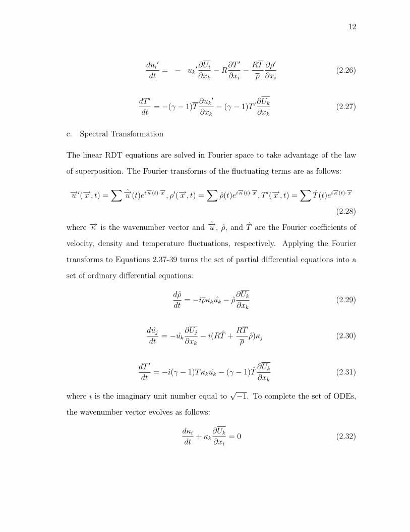
c. Spectral Transformation
The linear RDT equations are solved in Fourier space to take advantage of the law
of superposition. The Fourier transforms of the fluctuating terms are as follows:
−→u ′(−→x , t) =∑ −→u (t)ei
−→κ (t)·−→x , ρ′(−→x , t) =∑
ρ(t)ei−→κ (t)·−→x , T ′(−→x , t) =
∑T (t)ei
−→κ (t)·−→x
(2.28)
where −→κ is the wavenumber vector and −→u , ρ, and T are the Fourier coefficients of
velocity, density and temperature fluctuations, respectively. Applying the Fourier
transforms to Equations 2.37-39 turns the set of partial differential equations into a
set of ordinary differential equations:
dρ
dt= −iρκkuk − ρ
∂Uk∂xk
(2.29)
dujdt
= −uk∂Uj∂xk− i(RT +
RT
ρρ)κj (2.30)
dT ′
dt= −i(γ − 1)Tκkuk − (γ − 1)T
∂Uk∂xk
(2.31)
where ı is the imaginary unit number equal to√−1. To complete the set of ODEs,
the wavenumber vector evolves as follows:
dκidt
+ κk∂Uk∂xi
= 0 (2.32)

13
d. Particle Representation Method
From this point we may opt to directly solve Equations 2.41-44, and develop the
covariances of the fluctuating terms. However, for this work we choose to follow the
particle representation method presented in previous work by Kassinos and Reynolds
[19]. Accordingly, we define the conditional moments based on wavenumbers as:
Rij ≡ 〈u∗i uj|−→κ 〉 (2.33)
Lj ≡ 〈T ∗uj|−→κ 〉 (2.34)
Mj ≡ 〈ρ∗uj|−→κ 〉 (2.35)
A ≡ 〈ρ∗T |−→κ 〉 (2.36)
B ≡ 〈T ∗T |−→κ 〉 (2.37)
C ≡ 〈ρ∗ρ|−→κ 〉 (2.38)
Using Equations 2.41-2.43 we construct the evolution equations for the conditional
moments of the fluctuating field:
dRij
dt= −∂Ui
∂xkRkj −
∂Uj∂xk
Rik + ıR(Ljκi − L∗iκj) + ıRT
ρ(Mjκi − M∗
i κj) (2.39)
dMi
dt= ıρκkRki −
∂Uk∂xk
Mi −∂Ui∂xk
Mk − ıRAκi − ıRT
ρCκi (2.40)
dLidt
= ı(γ − 1)TκkRki − (γ − 1)∂Uk∂xk
Li −∂Ui∂xk
Lk − ıRBκi − ıRT
ρA∗κo (2.41)
dA
dt= ıρκkL
∗k − ı(γ − 1)TMkκk − γ
∂Uk∂xk
A (2.42)
dB
dt= −2(γ − 1)
∂Uk∂xk
B + ı(γ − 1)Tκk(L∗k − Lk) (2.43)
dC
dt= −2
∂Uk∂xk
C + ıρκk(M∗k − Mk) (2.44)

14
We use equations 2.51-56 to solve for the conditional covariances. By summing over all
the wavenumbers we obtain the second-order moments of the flucutations in physical-
space:
uiuj =∑
Rij(−→κ , t) (2.45)
uiT =∑
Li(−→κ , t) (2.46)
ρui =∑
Mi(−→κ , t) (2.47)
ρT =∑
A(−→κ , t) (2.48)
T 2 =∑
B(−→κ , t) (2.49)
ρ2 =∑
C(−→κ , t) (2.50)
There are two advantages to following this approach of summing over all the
wavenumbers: (i) it shows the clear correlation between several fluctuating moments
and (ii)solving over all wave numbers increases the accuracy and computational effi-
ciency. Since each of the covariances consist of real and imagimaginary components,
we end up with a set of 26 ordinary differential equations that are solved simultane-
ously. To step in time we utilize a fourth-order Runge-Kutta scheme.

15
B. Favre-Averaged Statistics
Here we present the development of the Favre-averaged RDT equations in a format
similar to that of Reynolds-averaged RDT.
1. Methodology
The pathway to derive the Favre-averaged fields is tangent to the approach outlined
in the previous section. Once again, we begin with the inviscid conservation equations
for compressible flow and the state equation for an ideal gas in a slightly different
format:
∂ρ
∂t+∂(ρUi)
∂xi= 0 (2.51)
∂(ρUi)
∂t+∂(ρUiUj)
∂xj= −∂P
∂xi(2.52)
∂(ρT )
∂t+∂(ρTUj)
∂xj= −P
cv
∂Uj∂xj
(2.53)
P = ρRT (2.54)
where γ is the ratio of specific heats. The equations that govern the instantaneous
flow field are the same as Reynolds-averaged RDT but when decomposing the field,
we now utilize density weighted-mean components for velocity and temperature as
shown below:
Ui =ρUiρ
+ ui′′
= Ui + ui′′
(2.55)
T =ρT
ρ+ T
′′= T + T
′′(2.56)

16
Reynolds decomposition is still applied to pressure and density variables. When
applying the decomposition to the governing equations for the instantaneous flow
field become:
∂ρ
∂t+
∂
∂xiρ(Ui + ui
′′) = 0 (2.57)
∂
∂tρ(Ui + ui
′′) +
∂
∂xj(ρ(Ui + ui
′′)(Uj + uj
′′)) = −R ∂
∂xiρ(T + T
′′) (2.58)
∂
∂tρ(T + T
′′) +
∂
∂xjρ(T + T
′′)(Uj + uj
′′) = −Rρ(T + T
′′)
cv
∂(Uj + uj′′)
∂xj(2.59)
P = ρR(T + T′′) (2.60)
Notice we have already substituted the ideal gas equation into the momentum and
energy equations. Taking the mean of these equations we find the conservation equa-
tions for the mean flow:
∂ρ
∂t+∂ρUi∂xi
= −∂ρ′ui
′′
∂xi(2.61)
∂(ρUi)
∂t+
∂
∂xj(ρUiUj + ρui
′′uj′′) = −R∂(ρT )
∂xi(2.62)
∂(ρT )
∂t+
∂
∂xj(ρT Uj + ρT ′′uj
′′)
= −Rcv
(ρT∂Uj∂xj
+ T ρ′∂uj
′′
∂xj+ ρT ′′ ∂uj
′′
∂xj+ ρT ′′ ∂uj
′′
∂xj) (2.63)
As shown in Reynolds-averaged RDT development, the governing fluctuation
equations are derived by subtracting the mean conservation equations from the in-

17
stantaneous flow field equations. Subtracting Equation 2.61 from Equation 2.57, the
fluctuating mass equation is:
∂ρ′
∂t+ Uj
∂ρ′
∂xj= −∂(ρui
′′)
∂xi− ρ′∂Ui
∂xi(2.64)
The fluctuating momentum equation, found by subtracting Equation 2.62 from Equa-
tion 2.58 is:
∂(ρui′′)
∂t+ Uj
∂(ρui′′)
∂xj= − ρui
′′ ∂Uj∂xj− ∂(ρ′Ui)
∂t
+∂
∂xj(ρui
′′uj′′ − ρ′UiUj − ρUiuj
′′ − ρui′′uj
′′
− ρ′Uiuj′′ − ρ′ui
′′uj
′′)
− R∂
∂xi(ρT
′′+ ρ′T + ρ′T
′′) (2.65)
We have already substituted the ideal gas equation into our momentum equation in
a previous step so it need not be done again. Instead, we now develop a second
momentum equation which solves for the first order velocity fluctuations:
ρ(∂ui
′′
∂t+ Uj
∂ui′′
∂xj) = − ui
′′(∂ρ
∂t+ Uj
∂ρ
∂xj)− ρui
′′ ∂Uj∂xj
− ρ′(∂Ui∂t
+ Uj∂Ui∂xj
)− ρuj′′ ∂Ui∂xj
− ρ∂
∂xj(ui
′′uj
′′)−R ∂
∂xi(ρT
′′)
− Rρ′′ ∂T
∂xi−RT ∂ρ
′
∂xi(2.66)
Finally we find the fluctuating energy equation by subtracting equation 2.63 from

18
Equation 6.59:
∂(ρT′′)
∂t+ Uj
∂(ρT′′)
∂xj= − (ρT
′′)∂Uj∂xj− ∂(ρ′T )
∂t
− ∂
∂xj(ρ′T Uj + ρTuj
′′+ ρuj
′′T
′′ − ρui′′uj ′′)
− R
cv(ρ′T
∂Uj∂xj
+ ρT∂uj
′′
∂xj+ ρT
′′ ∂Uj∂xj
+ ρT′′ ∂uj
′′
∂xj
− T ρ′∂uj
′′
∂xj− ρT ′′ ∂uj
′′
∂xj− ρT ′′ ∂uj
′′
∂xj) (2.67)
Equations 2.64-67 comprise the governing fluctuating equations for Favre-averaged
flow fields. Next, we continue to follow the Reynolds-averaged approach and apply
the important RDT assumptions to simplify this set of equations.
a. Homogeneity Assumption
Once again the homogeneity condition forces the mean thermodynamic variables and
the mean velociy gradient to be uniform in space:
∂T
∂xi=∂P
∂xi=
∂ρ
∂xi= 0 (2.68)
∂Uj∂xj
(−→x , t) =∂Uj∂xj
(t) (2.69)
Again, only in shear flows are the homogeneity requirements satisfied. The moments
of the thermodynamic and velocity fluctuation variables become spatially indepen-
dent:
∂
∂xiφ′φ′ =
∂
∂xiφ′φ′φ′ = ... = 0 (2.70)
Applying the homogeneity condition to Equations 2.64-67, we find the rapid distortion
equations for the Favre-averaged fluctuating fields to be:
∂ρ′
∂t+ Uj
∂ρ′
∂xj= −∂(ρui
′′)
∂xi(2.71)

19
∂(ρui′′)
∂t+ Uj
∂(ρui′′)
∂xj= − Ui(
∂ρ′
∂t+ Uj
∂ρ′
∂xj)− ρ′(∂Ui
∂t+ Uj
∂Ui∂xj
)
− ρUi∂uj
′′
∂xj− ρuj
′′ ∂Ui∂xj− Uiuj
′′ ∂ρ′
∂xj− ρ ∂
∂xj(ui
′′uj
′′)
− ui′′uj
′′ ∂ρ′
∂xj−Rρ∂T
′′
∂xi−RT ∂ρ
′
∂xi−R ∂
∂xi(ρ′T
′′) (2.72)
ρ(∂ui
′′
∂t+ Uj
∂ui′′
∂xj) = − ui
′′(∂ρ
∂t+ Uj
∂ρ
∂xj)− ρ′(∂Ui
∂t
+ Uj∂Ui∂xj
)− ρuj′′ ∂Ui∂xj− ρ ∂
∂xj(ui
′′uj
′′)
− R∂
∂xi(ρT
′′)−Rρ′′ ∂T
∂xi
− RT∂ρ′
∂xi(2.73)
∂(ρT′′)
∂t+ Uj
∂(ρT′′)
∂xj= − (
∂(ρ′T )
∂t+ Uj
∂(ρ′T )
∂xj)− ρT ∂uj
′′
∂xj
− T uj′′ ∂ρ′
∂xj− ρuj
′′ ∂T′′
∂xj− ρT ′′ ∂uj
′′
∂xj
− R
cv(ρT
∂uj′′
∂xj+ ρT
′′ ∂uj′′
∂xj− T ρ′∂uj
′′
∂xj
− ρT ′′ ∂uj′′
∂xj− ρT ′′ ∂uj
′′
∂xj) (2.74)
b. Linearization
Since RDT is a linear theory, the next step is to neglect all terms which are non-linear
in fluctuations. The linearized Favre-averaged fluctuating equations are:
dρ′
dt= −∂(ρui
′′)
∂xi(2.75)
d(ρui′′)
dt= −ρuj
′′ ∂Ui∂xj−R∂(ρT
′′)
∂xi−RT ∂ρ
′
∂xi(2.76)

20
d(ui′′)
dt= −uj
′′ ∂Ui∂xj− R
ρ
∂(ρT′′)
∂xi− RT
ρ
∂ρ′
∂xi(2.77)
d(ρT′′)
dt= −ρuj
′′ ∂T
∂xj− RρT
cv
∂uj′′
∂xj(2.78)
c. Spectral Transformation
Continuing along the same path as R-RDT development, we transforming the fluctu-
ating quantities to Fourier space in order to turn the above PDEs into ODEs:
dρ′
dt= −ıκmαm (2.79)
du′′i
dt= −u′′
m
∂Ui∂xm
− ıκiR
ρ(β + T ρ′) (2.80)
dαidt
= −αm∂Ui∂xm
− ıRκi(β + T ρ′) (2.81)
dβ
dt= −ı(γ − 1)ρTκmum
′′(2.82)
where the new Greek letters represent:
αi = ρui′′
(2.83)
β = ρT′′
(2.84)
Again, we close the set of ODE’s with the evolution of the wavenumber vector:
dκidt
+ κk∂Uk∂xi
= 0 (2.85)
d. Particle Representation Method
For Favre-averaged fields, the conditional moments based upon wavenumber are:
Aij = 〈u∗i uj|−→κ 〉 (2.86)

21
Bij = 〈α∗i αj|−→κ 〉 (2.87)
Cij = 〈α∗i uj|−→κ 〉 (2.88)
Di = 〈u∗i ρ|−→κ 〉 (2.89)
Ei = 〈α∗i ρ|−→κ 〉 (2.90)
Fi = 〈u∗i β|−→κ 〉 (2.91)
Gi = 〈α∗i β|−→κ 〉 (2.92)
H = 〈β∗ρ|−→κ 〉 (2.93)
I = 〈ρ∗ρ|−→κ 〉 (2.94)
J = 〈β∗β|−→κ 〉 (2.95)
The final step in development of Favre-averaged RDT is to construct the evolution
equations of the conditional moments using Equations 2.79-82. After doing so we
substitute in the appropriate labels above (Equations 2.86-95) and the fluctuating
moments for Favre-averaged fields are:
dAijdt
= −Amj∂Ui∂xm
− Aim∂Ui∂xm
+ ıκiR
ρ(F ∗j + TD∗j )− ıκi
R
ρ(Fi + TDi) (2.96)
dBij
dt= −Bmj
∂Ui∂xm
−Bim∂Uj∂xm
+ ıRκi(G∗j + TE∗j )− ıRκj(Gi + TEi) (2.97)
dCijdt
= −Cmj∂Ui∂xm
− Cim∂Uj∂xm
+ ıRκi(F∗j + TD∗j )− ıκj
R
ρ(Gi + TEi) (2.98)
dDi
dt= −Dm
∂Ui∂xm
+ ıκiR
ρ(H + T I)− ıκmC∗mi (2.99)
dEidt
= −Em∂Ui∂xm
+ ıRκi(H + T I)− ıκmBim (2.100)
dFidt
= −Fm∂Ui∂xm
+ ıκiR
ρ(J + TH∗)− ı(γ − 1)ρTκmAim (2.101)

22
dGi
dt= −Gm
∂Ui∂xm
+ ıRκi(J + TH∗)− ı(γ − 1)ρTκmCim (2.102)
dH
dt= ıκm[(γ − 1)ρTDm −G∗m] (2.103)
dI
dt= ıκm(Em − E∗m) (2.104)
dJ
dt= ı(γ − 1)ρTκm(Fm − F ∗m) (2.105)
Once again, by summing over all wavenumbers we obtain the second and third order
moments of the fluctuating field in physical space:
uiuj =∑−→κ
Aij(−→κ , t) (2.106)
αiαj =∑−→κ
Bij(−→κ , t) (2.107)
αiuj =∑−→κ
Cij(−→κ , t) (2.108)
uiρ =∑−→κ
Di(−→κ , t) (2.109)
αiρ =∑−→κ
Ei(−→κ , t) (2.110)
uiβ =∑−→κ
Fi(−→κ , t) (2.111)
αiβ =∑−→κ
Gi(−→κ , t) (2.112)
βρ =∑−→κ
H(−→κ , t) (2.113)
ρρ =∑−→κ
I(−→κ , t) (2.114)
ββ =∑−→κ
J(−→κ , t) (2.115)
These equations along with the wavenumber vector evolution equation make up
the set of 65 ODEs necessary to solve Favre-averaged RDT. It is clear to see that

23
almost all the equations are interdependent on one another, therefore we must obtain a
solution to the density-weighted turbulent kinetic energy using this averaging method.
As in the previous averaging approach, a fourth order Runge-Kutta scheme is used
to advance the solution in time.
C. Numerical Implementation and Validation
1. Numerical Implementation
In this section we will present the parameters and timescales that are utilized in this
research. Previous work on rapid distortion theory has looked at all different types
of flow deformation, but for this work we focus only on steady homogeneous shear
deformation, where the mean velocity gradient is presented as:
∂Ui∂xj
=
0 S 0
0 0 0
0 0 0
(2.116)
We generate initial conditions for the real and imaginary covariances as well as
the wavenumber vector in spectral space. We look at a collection of 6079 wavenumber
vectors which are evenly distributed across the surface of a unit sphere. This approach
is taken to ensure a statistical isotropic initial flow field. Initial velocity vectors
are chosen such that they are normal to the wavenumber vectors to enforce initial
incompressibility. To satisfy the dilatational initial conditions we make the amplitude
and wavenumber vectors parallel to one another. We set the initial thermodynamic
variables to standard values, density is set to ρ = 1.0 and mean temperature is set to
300K.
Previous studies have shown that one of the most relevant parameters of com-

24
pressible RDT is the gradient Mach number:
Mg ≡Sl√γRT0
(2.117)
where R is the universal gas constant, T0 is the initial temperature, and l is the
initial characteristic length that is equivalent to the magnitude of the wavenumber
vector. For low Mach number values the incompressible results are recovered(i.e.
Mg = 0.01), whereas for high Mach number values we recover the Burger’s limit
results(i.e. Mg = 2880).
For this study we choose to examine two other parameters: (i) the initial turbu-
lent Mach number Mt and (ii) the initial temperature fluctuation intensity Ts.
Mt =
√ui′ui′√γRT0
(2.118)
Ts =
√T ′T ′0
T0
(2.119)
These parameters are used to determine how initial thermodynamic and velocity
fluctuations influence the evolution of the turbulent flow field. The parameter values
for the different cases presented in this thesis are shown in Table I.
2. R-RDT Validation
Validation for R-RDT simulations against DNS results can be seen in previous works
[10, 13]. Yu & Girimaji [10] demonstrate that the R-RDT equations capture the
limiting cases of incompressible turbulence and pressure-released turbulence behavior
accurately. At the limit of vanishingly small Mg, they show that this R-RDT for-
mulation yields results identical to standard incompressible RDT results published,
for example, in Pope [1]. At the other extreme, in the limit of very large Mach
number, Yu & Girimaji show that R-RDT recovers known analytical solutions of

25
Table I. Case Parameter Values
Case Mg Mt Ts(%) Case Mg Mt Ts(%)
1 5 0.1 0 16 30 0.5 0
2 5 0.5 0 17 30 1.0 0
3 5 1.0 0 18 30 2.0 0
4 5 2.0 0 19 30 0.1 1
5 5 0.1 1 20 30 0.1 5
6 5 0.1 5 21 30 0.1 10
7 5 0.1 10 22 67 0.1 0
8 15 0.1 0 23 67 0.5 0
9 15 0.5 0 24 67 1.0 0
10 15 1.0 0 25 67 2.0 0
11 15 2.0 0 26 67 0.1 1
12 15 0.1 1 27 67 0.1 5
13 15 0.1 5 28 67 0.1 10
14 15 0.1 10 29 0.01 0.1 0
15 30 0.1 0 30 2880 0.1 0
pressure-released turbulence.
In the work by Lavin [13] the R-RDT approach is validated against DNS results.
Even though R-RDT only describes the linear processes of turbulence, it is shown
that it still captures the flow physics in the rapid limit as seen in Figures 3 and 4.
By examining the turbulent kinetic energy growth rate and the component of the
anisotropy tensor in the direction of shearing, we see that R-RDT produces similar
trends found in DNS results, but it is done with a small fraction of the computational
effort required by DNS.

26
Fig. 3. Turbulent kinetic energy growth rate for varying gradient Mach numbers Mg.
Plots are shown for (a)DNS (with solid line indicating Burgers limit and arrows
showing direction of increasing gradient Mach number) and (b) R-RDT (values
of Mg indicated as follows: ? : 0.72; ◦ : 1.00; 4 : 1.44; � : 2.88; � : 5.76; × :
14.4; N : 28.8; � : 288; � : 2880.)Produced by Tucker Lavin [13].
Fig. 4. b12 anisotropy component of initially-incompressible homogeneous turbulence
in pure shear for varying gradient Mach numbers Mg.Plots are shown for
(a)DNS (with solid line indicating Burgers limit and arrows showing direction
of increasing gradient Mach number) and (b) R-RDT (values of Mg indicated
as follows: ? : 0.72; ◦ : 1.00; 4 : 1.44; � : 2.88; � : 5.76; × : 14.4; N : 28.8;
� : 288; � : 2880.)Produced by Tucker Lavin [13].

27
Fig. 5. Evolution of turbulent kinetic energy for varying initial gradient Mach
numbers(Mg).
28
Fig. 6. b12 anisotropy component of initially-incompressible homogeneous turbulence
in pure shear for varying gradient Mach numbers Mg.
3. F-RDT Validation
Preliminary validation for this approach was first seen in Lavin [13] where compar-
ison of F-RDT and R-RDT results showed tremendous agreement. Lavin explains
this similarity by proving that the velocity mean and fluctuating components yield
the same values for both averaging approaches. As a result, the covariance of both
techniques are the same, leading to matching turbulent kinetic energy and internal
energy growth. Turning to Figure 5, our results from the F-RDT approach produces
the same turbulent kinetic energy growth rate pattern which is seen in previous R-
RDT and DNS studies. In Figure 6 we present the component of the anisotropy tensor
in the direction of shearing. By comparing this Figure 6 with Figure 4 we see that
the same basic trends are present. F-RDT even captures the trend seen in DNS of
the anisotropy tensor where the larger initial Mach numbers dip further and oscillate

29
after their maximum value. At this point, we can state that F-RDT performs at the
same level as R-RDT simulations. In Chapter IV of this thesis we present why F-
RDT is the superior choice in approaches when examining the linear processes found
in turbulence. Unless otherwise stated, only F-RDT will results will be presented
from this point onward. The parameters values for each case are presented in Table
I.
30
CHAPTER III
CHARACTERIZATION OF THREE-STAGE BEHAVIOR
It can be seen from previous works [10, 11, 12, 13] that key flow statistics - kinetic
energy, Reynolds stresses - of compressible homogeneous shear turbulence exhibit a
multistage temporal growth: (i) early time, (ii) intermediate time and (iii) asymptotic
state. The turbulent kinetic energy has been a key property of study in compressible
RDT [10, 11, 12, 13]. The three stages can also be labeled according to the growth rate
of kinetic energy. The three regimes are: (1) rapid growth stage equivalent to growth
exhibited by the pressure-released case, (2) a stabilization stage where energy growth
is nearly zero, (3) asymptotic regime of growth similar to incompressible flows. The
most complete explanation, to date, of the multi-stage evolution of rapidly sheared
compressible turbulence is provided by Cambon and co-workers in a series of articles
[3, 9]. Using a semi-analytical investigation, these authors provide a preliminary
explanation for the observed behavior at three distinct time regimes. The authors also
clearly distinguish the differences between compressible sheared and strained flows.
It is also shown the asymptotic linear effects may be independent of initial Mach
number, whereas the non-linear processes exhibit a stronger dependence. There is a
clear demonstration in these papers [3, 9] that the stabilizing effect of compressibility
in shear flows can be adequately explained with the linear Rapid Distortion Theory.
The stabilization is attributed to the feed-back of the dilatational disturbances upon
the solenoidal field [13].
In this chapter, we investigate the stabilization process in greater detail. We seek
to understand the three-stage behavior in terms of the changing role of pressure in
each regime. Important contributions in this regard has been made by Livescu [14]
who focuses on the level of anisotropy at different regimes. The focus of this work is

31
on the mechanisms in different stages. To further demarcate the three-regimes, we
examine the RDT evolution in three different timescales. Throughout this chapter
(unless otherwise stated) only Mg(0) is varied and Mt(0) is held constant at 0.1 for
different runs.
A. Three-Stage Behavior in Different Timescales
The three timescales used in the investigation are: (i) shear time, (ii) acoustic time
(at/l0), and (iii) mixed time (√
alot). We choose to view our results in this manner
because each timescale highlights different aspects of flow physics. First we examine
the evolution of kinetic energy in various timescales:
k =1
2ρui′ui′ (3.1)
Fig. 7. Evolution of normalized turbulent kinetic energy for varying initial gradient
Mach numbers(Mg) as seen in shear time for initial Mt = 0.1.

32
1. Shear Time
In previous studies, the majority of temporal evolution results are presented in shear
time (St) since the timescale is a directly related to the total shear applied to the
system. In this timescale the transition between stage 1 and Stage 2 is most evident.
This transition represents the ’peel-off’ of kinetic energy value from Burger’s limit
to the stabilization regime, as can be seen in Figure 7. These transition times are
consistent with that seen in Simone et. al.[9].
Fig. 8. Evolution of normalized turbulent kinetic energy for varying initial gradient
Mach numbers(Mg) as seen in acoustic time for initial Mt = 0.1.
2. Acoustic Time
The use of acoustic timescales (at = t ∗√γRT0) to display the multistage growth of
properties in compressible flow at the rapid distortion limit was first done in Lavin
[13] for the case of R-RDT. In Figure 8, we present F-RDT turbulent kinetic energy

33
evolution in acoustic time for different gradient Mach numbers. The acoustic timescale
has the advantage of clearly displaying the three-stage growth of turbulent kinetic
energy. Another advantage of the acoustic timescale is the clear demonstration of the
onset of the third regime. Figure 8 also shows the third and final regime is reached
at approximately two or three acoustic time units for all Mg cases. Again, further
study is presented later to support this observation.
Fig. 9. Evolution of normalized turbulent kinetic energy for varying initial gradient
Mach numbers(Mg) as seen in mixed time for initial Mt = 0.1.
3. Mixed Time
The mixed timescale is the geometric average of the shear and acoustic time scales
( St√Mg
). We introduced this timescale as another option to clearly display the three-
stage turbulent kinetic energy evolution. The main benefit of this normalization is
that the onset of regime 2 is at an identical time for all Mach numbers considered.

34
4. Regimes of Evolution
Inspections of Figures 8 and 9 show the approximate time demarcations between the
three regimes of behavior.
Regime 1: 0 < St < 1− 2√Mg
Regime 2: 1− 2√Mg < at < 1− 3
Regime 3: at > 3
The exact demarcation between the various regimes and the physics within each
regime will be addressed later.
Fig. 10. Evolution of gradient Mach number in shear time-scale.
B. Evolution of Gradient and Turbulent Mach Numbers
As the turbulence field evolves from its initial conditions, both Mg (gradient Mach
number) and Mt (turbulent Mach number) evolve from their initial values. It is
instructive to examine the evolution of these Mach numbers as a function of time.
In Figures 10, 11 and 12, the evolution of the gradient Mach number is shown in
different time scales. By examining the evolution of Mg in shear time, it is clear that

35
Fig. 11. Evolution of gradient Mach number in acoustic time-scale.
Fig. 12. Evolution of gradient Mach number in mixed time-scale.

36
within one shear time, the initial gradient Mach number value begins to significantly
decrease. It is very interesting to note that within one acoustic time (Fig. 11), the
gradient Mach number is nearly one for all initial Mg values. After one acoustic time,
the evolution of the gradient Mach number is confined to the path laid out in Figure
11. From these figures, it is possible to determine the value range of the gradient
Mach number in each regime.
In Figures 13, 14, and 15 the evolution of the initial turbulent Mach number
is presented in the different timescales. In shear time, it is important to note that
after four shear times, the growth of all initial turbulent Mach numbers decreases
significantly. In acoustic time, the 3-regime evolution is clearly seen, but no significant
alignment of all cases is present. The evolution of the initial turbulent Mach number
is best displayed in mixed time due to the fact that both the 3-regime growth is
evident and all runs align where the initial values begin to show significant growth.
C. Physics of Different Regimes
The objective in this section is to perform a careful analysis of the various physical
processes in each regime. We are especially interested in the changing role of pressure.
To examine the physical processes we study the linearized Reynolds-Stress evolution
equation (e.g. Pope [1]).
dρui”uj”
dt= Pij + Πij
(r) (3.2)
where Pij is the production tensor and Πij(r) is the rapid pressure-strain correlation
tensor. In linear analysis, the evolution of the Reynolds-stresses is influenced purely
by the inertial effects (Pij) and the pressure effects (Πij(r)). As mention in the in-
troduction to this thesis, the rapid pressure-strain correlation is one of the terms
that require improved closure modeling. In this section we will determine the role of

37
Fig. 13. Evolution of turbulent Mach number in shear time-scale for zero initial tem-
perature fluctuations and an initial Mg = 5.
Fig. 14. Evolution of turbulent Mach number in acoustic time-scale for zero initial
temperature fluctuations and an initial Mg = 5.

38
Fig. 15. Evolution of turbulent Mach number in mixed time-scale for zero initial tem-
perature fluctuations and an initial Mg = 5.
the rapid pressure-strain correlation in each regime by studying the evolution of the
production tensor and the time rate of change of the Reynolds stresses.
We first present the evolution of Reynolds-stress growth rate and production in
all three time scales in Figures 16, 17 and 18. In all timescales, the three-regime
evolution is easily seen. Once again each timescale highlights different features. In
Figure 16 which displays the results in shear time, we notice how the smaller initial
gradient Mach number cases seem to ”peel-off” a high Mach number path, similar in
manner to the first regime in the evolution of turbulent kinetic energy. We present
the evolutions in acoustic time in Figure 17 where we can see that regardless of the
initial gradient Mach number, the evolution of production and the growth rate of the
Reynolds stresses all evolve along the same path in the final regime. For the mixed
timescale, seen in Figure 18, all the maximum peaks align at one mixed time unit. In

39
Fig. 16. Evolution of production and time rate of change of reynolds stresses in shear
time-scale for Mg = 5.
Fig. 17. Evolution of production and time rate of change of reynolds stresses in acoustic
time-scale for Mg = 5.

40
Fig. 18. Evolution of production and time rate of change of reynolds stresses in mixed
time-scale for Mg = 5.
order to determine the role of pressure in each regime, we must examine each regime
individually.
1. Regime 1
When examining the first regime of production evolution and Reynolds-stress growth,
the nature of pressure is most clearly seen by studying the P11 and u1u1 components.
In Figure 19, the production and Reynolds-stress growth lines are nearly identical
throughout the majority of the first regime. Using Equation 3.2 we can surmise
that the role of the pressure strain correlation, and therefore the role of pressure
itself, is negligible in this regime. We see that before we get to a mixed time of
1, the production and Reynolds-stress growth lines start to diverge for the smaller
initial gradient mach numbers. This separation indicates that pressure begins to
play a more significant role in the flow field physics. The moment of separation of
production and Reynolds-stress growth coincides with the ”peel-off” seen in the first

41
regime of turbulent kinetic energy evolution. Thus, we can conclude that in the first
regime, the effect of advection dominates pressure yielding a behavior identical to the
pressure-released or Burger’s limit turbulence.
Fig. 19. Evolution of production and time rate of change of Reynolds stresses in mixed
time-scale during the first stage of evolution.
By examining other statisical quantities of the flow field we can gain a better
understanding of the physics involved in the first regime of growth. In Figure 20,
the evolution of the pressure fluctuations moment is presented in mixed time. As
expected from the examination of Figure 19 the fluctuating pressure experiences zero
growth during this regime. Towards the end of the first regime the fluctuating pres-
sure obtains non-zero values but they are still small. The study the evolution of the
dilatational kinetic energy and the internal energy is shown in Figures 21 & 22. The
dilatational kinentic energy remains at a constant non-zero value throughout the ma-
jority of the first regime where as the internal energy obtains a non-zero value toward
the end of this regime. It is clear that the partition between these energies heavily
favors the dilatational kinetic energy.

42
Fig. 20. Evolution of fluctuating pressure moment in mixed time-scale during the first
stage of evolution.

43
Fig. 21. Evolution of dilatational kinetic energy in mixed time-scale during the first
stage of evolution.

44
Fig. 22. Evolution of the increment in thermal energy in mixed time-scale during the
first stage of evolution.
2. Regime 2
For regime 2, the overall picture is best demonstrated by examining P12 and the
growth of u1u2. The evolution of these quantities is shown in Figure 23. Unlike in
the previous regime, the production and Reynolds-stress growth rate no longer co-
incide. Although the magnitude of production is very large, the u1u2 growth rate
oscillates about zero, implying that the overall Reynolds-stress growth is zero during
this regime. Again, referring to Equation 3.2, we can infer that the pressure-strain
correlation term is working to nullify the production. Relating this back to the tur-
bulent kinetic energy evolution, this regime where pressure fights the inertial physics
coincides with the stabilization regime. Since there is non-zero growth in the final
regime, the second regime acts a buffer region between negligible pressure effects in
the first regime and the final role of pressure in the third regime.

45
Fig. 23. Evolution of production and time rate of change of Reynolds stresses in mixed
time-scale during the second stage of evolution.
Again, we examine the same flow field statistical quantities as regime 1 to under-
stand more of the physics associated with this regime. In Figure 24, the evolution of
the fluctutating pressure moment is displayed for the second regime. In this regime,
the fluctuating pressure experiences oscillatory growth. By comparing Figures 23 &
24 we see that the fluctuating pressure moment and production term are oscillating
in phase to one another. The figures support our previous conclusion that pressure is
working against production to stabilize the growth of the Reynolds-stresses by show-
ing that production evolves toward more negative values and the pressure fluctuating
moment evolves toward more positive values.
Examining the dilational kinetic energy and the increase in thermal energy in
Figures 25 and 26, we notice that these statistical quantities move away from their
initial values.

46
Fig. 24. Evolution of fluctuating pressure moment in mixed time-scale during the sec-
ond stage of evolution.

47
Fig. 25. Evolution of dilatational kinetic energy in mixed time-scale during the second
stage of evolution.
Fig. 26. Evolution of the increment in thermal energy in mixed time-scale during the
second stage of evolution.
48
3. Regime 3
The final regime of evolution is best examined in terms of P1,1 and Π1,1 as seen in
Figures 27 & 28. The most important feature is that the behavior of all gradient
mach number cases is nearly identical. This is in complete contrast to the previous
regimes in which Mg(0) played a significant role. The collapse of the results is also
consistent with the fact that the Mg(t) at these times is independent of Mg(0). It is
also seen that this behavior is similar to that of incompressible flows as seen in Figure
29. In summary, the pressure-strain correlation in this regime is similar to that of
incompressible turbulence. This finding lends quantitative support to the conclusions
of Simone et. al. [9].
Fig. 27. Evolution of rapid pressure-strain correlation term in mixed time-scale during
the third stage of evolution.

49
Fig. 28. Evolution of the production term in mixed time-scale during the third stage
of evolution.

50
Fig. 29. Evolution of rapid pressure-strain correlation and production terms in the
incompressible limit, shown in mixed time-scale.

51
To gain a greater understanding of the third regime, we look at the evolution
of the pressure fluctuations. We previously discussed the oscillatory nature of the
evolution of the pressure fluctuations in the second regime. This implies that the
pressure fluctuations in the second regime are governed by the wave equation. In
the third regime however, we observed that the production and rapid pressure-strain
correlation terms evolve in a manner similar to the incompressible limit. This suggests
that the pressure fluctuations are governed by the rapid part of Poisson’s equation:
∇2p(r) = −2ρ∂Ui∂xj
∂u”j
∂xi(3.3)
We examine the evolution of Poisson pressure in several different Mg cases in Figure
30. We note that even though the Poisson pressure fluctuations are large initially,
within three acoustic times, Poisson pressure has evolved to near zero values. With
our previous conclusions in mind, we plot the evolution of the pressure fluctuations
from the compressible RDT method, governed by Eq. 2.75, expecting all cases to
tend toward a near zero value. However, we discover that the compressible pressure
fluctuation settle to a value of unity as seen in Figure 31. We note that the com-
pressible fluctuations settle about a constant value after 2-3 acoustic times, which
shows agreement with Poisson pressure agreement. To finish our analysis we must
determine what causes the compressible pressure fluctuations to settle at unity and
not zero.
We previously deduced that the wave equation governs the second regime of
evolution for all flow field properties. We also mentioned that the frequency of the
wave oscillations increases in time and the oscillations continue into the third regime
of evolution. Based on this understanding, it is evident that there are still residual
wave effects occurring in the third regime where Poisson’s equation dominates as the
governing equation. Following this logic, we subtract the pressure fluctuations pro-

52
Fig. 30. Evolution of Poisson pressure fluctuations in the acoustic time-scale.
Fig. 31. Evolution of compressible pressure fluctuations in the acoustic time-scale.

53
Fig. 32. Evolution of residial pressure fluctuations in the acoustic time-scale.
duced by Poisson’s equation from the compressible pressure fluctuations to produce
the residual pressure fluctuations:
p′p′(res.) =p′p′(c) − p′p′(w)
ρ2γRTu”2u
”2(t)
(3.4)
We find agreement between the residual pressure fluctuations produced by the com-
pressible RDT method and the Poisson equation approach by comparing Figure 30
and Figure 32. It can be deduced from this agreement that the third regime of evo-
lution is governed by Poisson’s equation as in incompressible fluid flow but it still
maintains residual wave pressure produced in the second regime.

54
CHAPTER IV
POLYTROPIC COEFFICIENT
Earlier, we developed two different compressible RDT approaches, Reynolds-averaged
and Favre-averaged, for homogeneous shear flow and presented validation of both
approaches against DNS results. We claimed the F-RDT approach was more accurate
for thermodynamic quantities. We now present evidence of this statement until this
section.
The validation of the F-RDT approach for thermodynamic fluctuations is given
by examining the evolution of the polytropic coefficient for different initial turbulent
Mach numbers. The polytropic coefficient quantifies the relationship between the
pressure and density fluctuations:
n ≡
√p′p′/p2
ρ′ρ′/ρ2 (4.1)
Blaisdell [6] clearly demonstrates using DNS data that the polytropic coefficient shoud
be approximately equal to the specific heat ratio of the medium ( 1.4). In Figure 33
the evolution of the polytropic coefficient is shown for several initial turbulent Mach
numbers. Using R-RDT computations, as the value of the initial turbulent Mach
number increases, the polytropic coefficient tends away from the expected value. In
fact, it attains values close to zero close to zero at late times. Clearly this behavior is
unphysical. In Figure 34 the FRDT results for the polytropic coefficient of different
initial turbulent Mach numbers are presented. Unlike the R-RDT results, the F-RDT
results remain close to the expected value of 1.4 regardless of the magnitude of the
initial turbulent Mach number. Thus, F-RDT is the more appropriate choice for
examining compressible RDT for homogeneous shear flows because it captures the
thermodynamic aspects of flow physics better than R-RDT.

55
Fig. 33. Evolution of Averaged Polytropic coefficent for large initial turbulent Mach
numbers for Mg = 5 via R-RDT approach.

56
Fig. 34. Evolution of Averaged Polytropic coefficent for large initial turbulent Mach
numbers for Mg = 5 via F-RDT approach.

57
CHAPTER V
EFFECT OF THERMODYNAMIC FLUCTUATIONS
All previous studies involving the R-RDT and F-RDT approaches have all examined
simulations where all the thermodynamic fluctuating quantities were initially zero
and the initial turbulent Mach number was small( 0.004)[10, 13]. However, in re-
alistic applications thermodynamic fluctuations can be substantial. In this chapter
we investigate the effect of initial thermodynamic and velocity fluctuations on the
evolution of the flow field statistics.
A. Kinetic Energy
We already presented a detailed analysis of the three-regime evolution of turbulent
kinetic energy in Chapter III. Now we attempt to understand the effect of initial
temperature fluctuations and the initial turbulent Mach number on the three-regime
evolution.
1. Initial Temperature Fluctuation Intensity
We now investigate the influence of initial thermodynamic fluctuations. The results
shown in Figure 35 are cases for which the initial temperature fluctuations are 0, 1, 5
and 10 percent of the initial mean temperature value. It is evident from Figure 35 that
small temperature fluctuations have very little influence on the three regime evolution.
However large initial temperature fluctuations heavily influence the evolution of the
flow field by delaying the onset of the second regime where the growth stabilization
occurs. This effect is important because it implies that large initial temperature
fluctuations have the same influence as increasing the initial gradient Mach number.
Since all the thermodynamic variables are linked by the state equation of an ideal
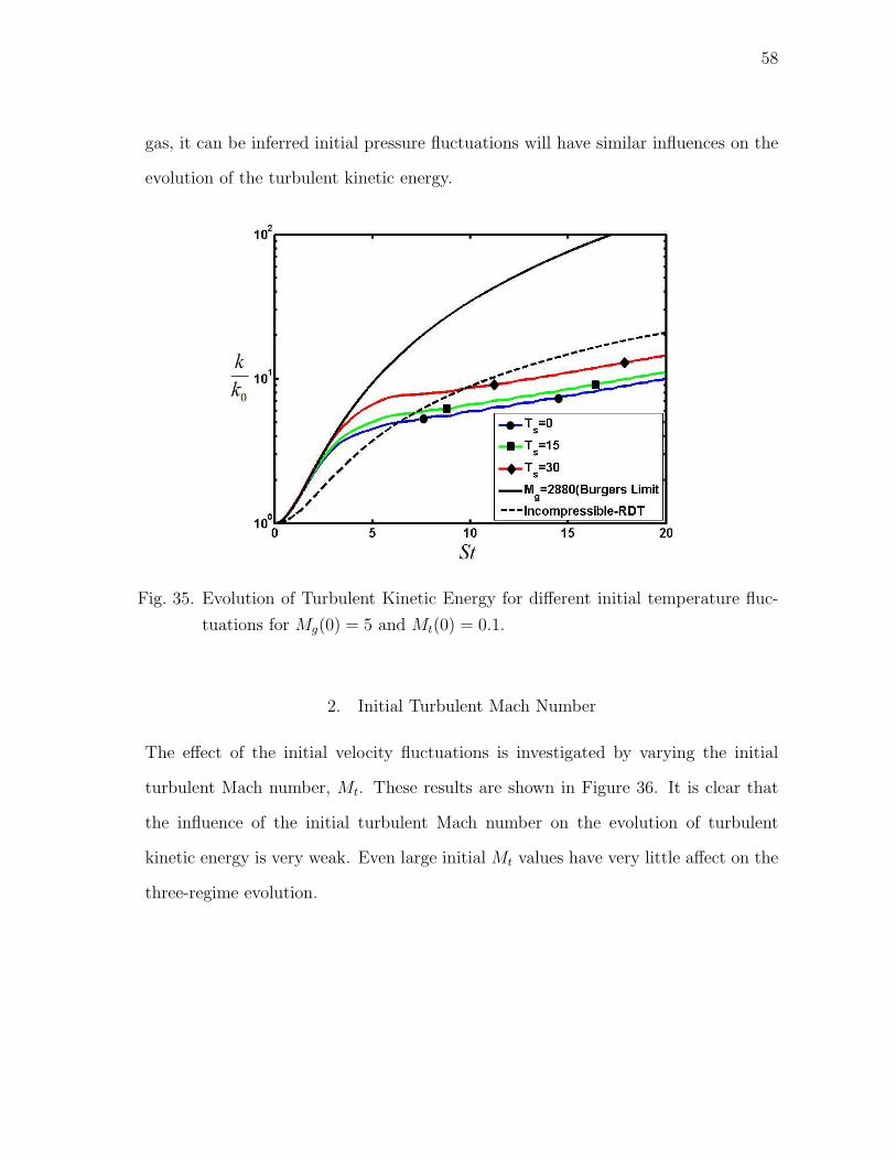
58
gas, it can be inferred initial pressure fluctuations will have similar influences on the
evolution of the turbulent kinetic energy.
Fig. 35. Evolution of Turbulent Kinetic Energy for different initial temperature fluc-
tuations for Mg(0) = 5 and Mt(0) = 0.1.
2. Initial Turbulent Mach Number
The effect of the initial velocity fluctuations is investigated by varying the initial
turbulent Mach number, Mt. These results are shown in Figure 36. It is clear that
the influence of the initial turbulent Mach number on the evolution of turbulent
kinetic energy is very weak. Even large initial Mt values have very little affect on the
three-regime evolution.

59
Fig. 36. Evolution of Turbulent Kinetic Energy for various initial turbulent Mach num-
bers with initial Mg = 5 and zero initial temperature fluctuations.
B. Equi-Partition Function
One of the chief findings of Lavin et. al. [11] was that there was equi-partition between
the dilatational kinetic energy and the increment in thermal energy. To investigate
the influence of initial thermodynamic and velocity fluctuations further we examine
the evolution of the equi-partition function:
φ ≡ ρu2”u2
”
2cvρ(T − T 0)(5.1)
where T 0 denotes the initial mean temperature. Here ρu2”u2
” is the dilatational
energy. For a value of φ = 1, there is a perfect equi-partition between the energy
modes.

60
1. Initial Temperature Fluctuation Intensity
In Figure 37 the evolution of the equi-partition function for initial temperature fluctu-
ation cases is presented. Once again, the strong influence of initial temperature fluctu-
ations is evident. Large initial temperature fluctuations cause the partition function
to be greater than unity as dilatational fluctuations are generated due to thermal
expansion. The larger initial temperature fluctuations, the greater the dilatational
energy produced at the initial time. In time, the partition function oscillates about
unity indicating a harmonic oscillator type of interaction between thermal and kinetic
energies. As time passes the magnitude of the oscillation decreases and equi-partition
is achieved.
Fig. 37. Evolution of equi-partition for large initial temperature fluctuations with ini-
tial Mg = 5 and initial Mt = 0.1.

61
2. Initial Turbulent Mach Number
The evolution of the equi-partition function for various initial turbulent Mach num-
bers is shown in Figure 38. The influence of the turbulent Mach number on the
evolution of the equi-partition is nearly negligible.
Fig. 38. Evolution of equi-partition function for various initial turbulent Mach num-
bers with initial Mg = 5 and zero initial temperature fluctuations.
C. Influence on Transition Times
Finally, we examine the influence of thermodynamic fluctuations on the three-stage
behavior. The two quantities of interest are: (i)Regime 1-2 transition time and (ii)
Regime 2-3 transition time.

62
1. Regime 1-2 Transition Time
This transition time refers to the point in the evolution of turbulent kinetic energy
where it peels off of the pressure-released (Burger’s turbulence) evolution path. This
point is important because it marks the end of the first regime of evolution and
the beginning of the second regime. We already stated that the Burger’s peel-off
time is influenced by the initial gradient Mach number. Now we seek to determine
the influence of initial thermodynamic fluctuations on this time. Peel-off times were
found for a range of initial conditions.
Fig. 39. Regime 1-2 transition times for various initial temperature fluctuations in
terms of mixed time.
For a constant initial turbulent Mach number (Mt = 0.1) the results are presented
in Figure 39. Larger initial temperature fluctuations cause the Burger’s peel-off time
to occur later, which agrees with Section 1 of this chapter. Even though it is evident
that the Burger’s peel-off time is dependent on the initial temperature fluctuations,

63
the exact relationship has yet to be determined.
Fig. 40. Regime 1-2 transition times for various Mt values in terms of mixed time.
The results for zero initial temperature fluctuations are presented in Figure 40.
This figure is very important in demonstrating the influence of the initial gradient
Mach number on Burger’s peel-off time. It is clear that transition time is not influ-
enced by the value of the initial turbulent Mach number. Second, the slope of the
lines implies a proportional relationship between Burger’s peel-off time and the initial
gradient Mach number (i.e. St ≈ C ∗√Mg).
2. Regime 2-3 Transition Time
This transition time refers to the point where the role of pressure becomes similar
to the incompressible flow behavior. We previously suggested that all cases have
reached the incompressible regime by one acoustic time. It is important to note

64
that the transition for each case represents the time when the evolution of each case
becomes parallel to the evolution of the incompressible limit case. Therefore, these
times occur after the incompressible limit has started.
Fig. 41. Regime 2-3 transition times for various initial temperature fluctuations in
terms of acoustic time.
For the constant initial turbulent Mach number cases(Mt = 0.1), the results are
displayed in Figure 41. For the smaller initial gradient Mach numbers, a clear re-
lationship between the incompressible limit time and initial temperature fluctuation
cannot be found. What is of interest in Figure 41 is how the larger initial gradient
Mach number values seem to collapse to a value of 2-3 acoustic times. This dis-
covery supports our claim that regardless of initial conditions, the evolution of the
turbulent kinetic energy for compressible RDT will reach the final evolution regime
at approximately one acoustic time.
In Figure 42, we present the results of the incompressible limit time for cases of

65
Fig. 42. Regime 2-3 transition times for various initial Mt values in terms of acoustic
time.

66
zero initial temperature fluctuations. Again we see that higher initial gradient Mach
numbers support our claim that initial conditions weakly, if at all, influence the onset
of the incompressible evolution regime. Another interesting finding in Figure 42 is
how the different initial turbulent Mach number cases don’t collapse on the same
line for larger initial gradient Mach numbers, suggesting that the transition to the
final regime may be slightly influenced by the initial turbulent Mach number. For
larger gradient Mach numbers, the second transition has occurred by 3-4 acoustic
time units.

67
CHAPTER VI
CONCLUSIONS
The effect of compressibility on shear driven turbulence is of great interest in hyper-
sonic flight applications. It has been known for several years that compressibility has
a stabilizing influence and reduces turbulence intensity and mixing. There have been
some explanations of the underlying processes using rapid distortion theory (RDT).
In this work, a comprehensive demonstration of the stabilizing mechanism is pre-
sented. The influence of thermodynamic fluctuations on the stabilizing physics is
also investigated.
While previous works have employed Reynolds-averaged RDT, here we also use
Favre-averaged RDT. The advantage of F-RDT is a more accurate representation of
thermodynamic variables. The most important findings of the work are now summa-
rized.
A. F-RDT Validation
F-RDT results of homogeneous shear compressible turbulence is compared against
direct numerical simulation data and R-RDT analysis for intermediate Mach number
values. Comparison is made for the kinetic energy growth rate, λ, and b12 anisotropy
component. F-RDT shows good agreement with the trends of both DNS and R-RDT
analysis for the range of initial gradient Mach numbers. The high Mach number
(Mg = 30, 67) display similar trends throughout, including the oscillatory motion
after the maximum peak. F-RDT shows a higher level of accuracy compared to
R-RDT when initial velocity fluctuations were introduced. F-RDT achieves values
near or at the expected value of the polytropic coefficient (≈ 1.4) for high levels of
initial velocity fluctuations whereas the accuracy of R-RDT analysis deteriorates as

68
the intensity of fluctuations increases.
B. Three timescales
The necessity of investigating evolution in three timescales - shear, acoustic, and
mixed - is presented. Each timescale highlights the three-regime evolution of the flow
field statistical quantities differently and therefore each timescale has advantages and
disadvantages. The main advantage of shear time is the clear transition from regime
1 to regime 2. The precise point of departure from pressure-released turbulence is
evident. Shear time also has the disadvantage of only showing two regimes clearly.
The acoustic timescale shows all three regimes clearly. It also is beneficial in iden-
tifying the expected transition to the third regime (≈ 1 acoustic time). Finally, the
geometric mixed time has the advantage of clearly pin-pointing the beginning of the
second regime.
C. Three-Regime Evolution
All the statistical quantities of the flow field exhibit a three-regime evolution trend.
By examining the evolution of the kinetic energy, the three regions of growth are
classified as: (i)rapid growth along the pressure released limit which lasts between
1-2 mixed time units and the gradient Mach number is greater than one, (ii) near-zero
growth regime which is complete within one acoustic time when the value of Mg is
about unity, and (iii) asyptotic growth similar in trend to the incompressible limit
where the gradient Mach number much less than one.

69
D. Role of Pressure in Three Regimes
The underlying physics in each regime was investigated using the linearized Reynolds-
stress evolution equation. The role of the pressure-strain correlation in each regime is
as follows: (i) pressure plays a negligent role as production and Reynolds-stress growth
rate maintain the same value, (ii)pressure works to nullify the production since the
Reynolds-stress growth rate is nearly zero and the magnitude of production is nonzero,
(iii) pressure plays a role similar to that of incompressible RDT since the evolution
of production and Reynolds-stress growth rate all fall along same path regardless of
initial gradient Mach number. Further investigation suggests that pressure evolution
in the third regime is governed by Poisson’s equation with residual wave effects from
the second evolution regime.
E. Effect of Thermodynamic Fluctuations
Analysis of different initial intensities of flow and thermodynamic fluctuations was
conducted. Results show the thermodynamic fluctuations have a strong influence on
the evolution of the flow field statistics whereas the initial velocity fluctuations only
weakly influence the development of the flow field statistics.
F. Transition Times
The final study conducted was to examine the influence of initial flow field fluctuation
on the two transition times of the three-regime evolution: (i) Regime 1-2 transition
and (ii)Regime 2-3 transition. Initial thermodynamic fluctuations have the affect
of delaying the onset of the second regime so Regime 1-2 transition occured later
for larger fluctuations. Initial velocity fluctuations showed no effect on Regime 1-
2 transition as all cases fell on the same path regardless of initial turbulent Mach

70
number. Regime 2-3 transition presented no clear qualitative influence from initial
flow field fluctuations for smaller gradient Mach numbers. However, larger initial
gradient Mach numbers delayed the second transition time to 3-4 acoustic time units.

71
REFERENCES
[1] S. B. Pope, Turbulent Flows. New York, NY: Cambridge University Press, 2000.
[2] G. K. Batchelor and I. Proudman, “The effect of rapid distortion of a fluid in
turbulent motion,” Q. J. Mech. Appl. Math.,vol. 7, no. 1, pp.121-152, 1954.
[3] C. Cambon, G. N. Coleman and D. N. N. Mansour, “Rapid distortion analysis
and direct simulation of compressible homogeneous turbulence at finite Mach
number,” J. Fluid Mech., vol. 257, pp. 641-665, 1993.
[4] G. Brethouwer, “The effect of rotation on rapidly sheared homogeneous turbu-
lence and passive scalar transport, linear theory and direct numerical simula-
tions,” J. Fluid Mech., vol. 542, pp. 305-342, 2005.
[5] P.A. Durbin and O. Zeman, “Rapid distortion theory for homogeneous com-
pressed turbulence with application to modeling,” J. Fluid Mech., vol. 242, pp.
349-370, 1992.
[6] G. A. Blaisdell, G. N. Coleman and N. N. Mansour, “Rapid distortion theory
for compressible homogeneous turbulence under isotropic mean strain,” Phys.
Fluids, vol. 8, pp. 2692-2705, 1996.
[7] G. N. Coleman and N. N. Mansour, “Simulation and modeling of homogeneous
compressible turbulence under isotropic mean compression,” in Symposium on
Turbulent Shear Flows. 8th, Munich, Federal Republic of Germany; 9-11 Sept.,
1991. pp. 21-3-1 to 21-3-6, 1991.
[8] L. Jacquin, C. Cambon and E. Blin, “Turbulence amplification by a shock wave
and rapid distortion theory,” Phys. Fluids A, vol. 5, no. 10, pp. 2539-2550, 1993.
72
[9] A. Simone, G. N. Coleman and C. Cambon, “The effect of compressibility on
turbulent shear flow: A rapid distortion theory and direct numerical simulation
study,” J. Fluid Mech., vol. 330, pp. 307-338, 1997.
[10] H. Yu and S. S. Girimaji, “Extension of compressible ideal-gas RDT to general
mean velocity gradients.” Phys. Fluids, vol. 19, no.4, pp. 041702, 2007.
[11] S. Suman, S. S. Girimaji, H. Yu and T. Lavin, “Rapid distortion of Favre-
averaged Navier-Stokes equations.” Submitted for publication to J. Fluid Mech.,
in 2010.
[12] S. Suman, S. S. Girimaji and R. L. Bertsch, “Homogeneously-sheared compress-
ible turbulence at rapid distortion limit: Interaction between velocity and ther-
modynamic fluctuations.” Turbulence, Heat and Mass Transfer 6, K. Hanjalic,
Y. Nagano,and S. Jakirlic Eds. New York: Begell House Inc., pp. 583-586, 2009.
[13] T. Lavin, Reynolds and Favre-Averaged Rapid Distortion Theory for Compress-
ible, Ideal Gas Turbulence. M. S. thesis. College Station: Texas A&M University.
2007.
[14] D. Livescu and C. K. Madnia, “Small scale structure of homogeneous turbulent
shear flow.” Phys. Fluids, vol. 16, no. 8, pp. 2864-2876, 2004.
[15] A. M. Savill, “Recent developments in rapid distortion theory.” Ann. Rev. Fluid
Mech. vol. 19, pp. 531-573, 1987.
[16] J. C. R. Hunt and D. J. Carruthers, “Rapid distortion theory and the ‘problems’
of turbulence.” J. Fluid Mech., vol. 212, pp. 497-532, 1990.
[17] S. S. Girimaji, J. R. O’Neil and D. Yu, “Rapid distortion analysis of homogeneous
turbulence subjected to rotating shear.” Phys. Fluids, vol. 18, no. 8, art. no.

73
085102, 2006.
[18] G. N. Coleman and N. N. Mansour, “Modeling the rapid spherical compression
of isotropic turbulence.” Phys. Fluids A, vol. 3, pp. 2255-2259, 1991.
[19] S. C. Kassinos and W. C. Reynolds, “A particle representation model for the
deformation of homogeneous turbulence.” Annual Research Briefs, Center for
Turbulence Research, NASA Ames/Stanford University, pp. 31-53, 1996.
[20] S. S. Girimaji, E. Jeong and S. V. Poroseva, “Pressure-strain correlation in ho-
mogeneous anisotropic turbulence subject to rapid strain-dominated distortion.”
Phys. Fluids, vol. 15, no. 10, pp. 3209-3222, 2003.
[21] S. Sarkar, “The stabilizing effect of compressibility in turbulent shear flow.” J.
Fluid Mech., vol. 282, pp. 163-186, 1995.

74
VITA
Rebecca Lynne Bertsch was born in Minneapolis, MN, USA. She received her
B.A. in physics from Colorado College in May 2007. She began her graduate studies
in aerospace engineering at Texas A&M University in August 2007 and graduated
with her M.S. in August 2010. She plans to pursue her doctoral degree at Texas
A&M University, focusing on the area of compressible turbulence modeling. She
can be contacted through Dr. Girimaji at Texas A&M University, Department of
Aerospace, H.R. Bright Building, Rm. 701, Ross Street - TAMU 3141, College Station
TX 77843-3141.
The typist for this thesis was Rebecca Bertsch.