Embed Size (px)
Citation preview
Berendt: Knowledge and the Web, 2014, http://www.cs.kuleuven.be/~berendt/teaching/
1
Knowledge and the Web –
Exploring your data and testing your hypotheses:
Data analysis (not only KDD) II
Bettina Berendt
KU Leuven, Department of Computer Science
http://people.cs.kuleuven.be/~bettina.berendt/teaching
Last update: 26 November 2014
Berendt: Knowledge and the Web, 2014, http://www.cs.kuleuven.be/~berendt/teaching/
2
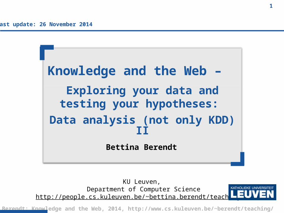
Phases talked about today
Berendt: Knowledge and the Web, 2014, http://www.cs.kuleuven.be/~berendt/teaching/
3
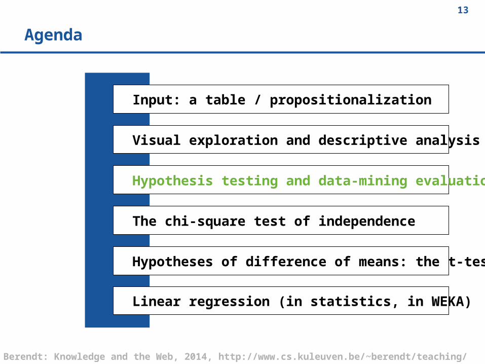
Agenda
Input: a table / propositionalization
Visual exploration and descriptive analysis
Hypothesis testing and data-mining evaluation
The chi-square test of independence
Hypotheses of difference of means: the t-test
Linear regression (in statistics, in WEKA)
Berendt: Knowledge and the Web, 2014, http://www.cs.kuleuven.be/~berendt/teaching/
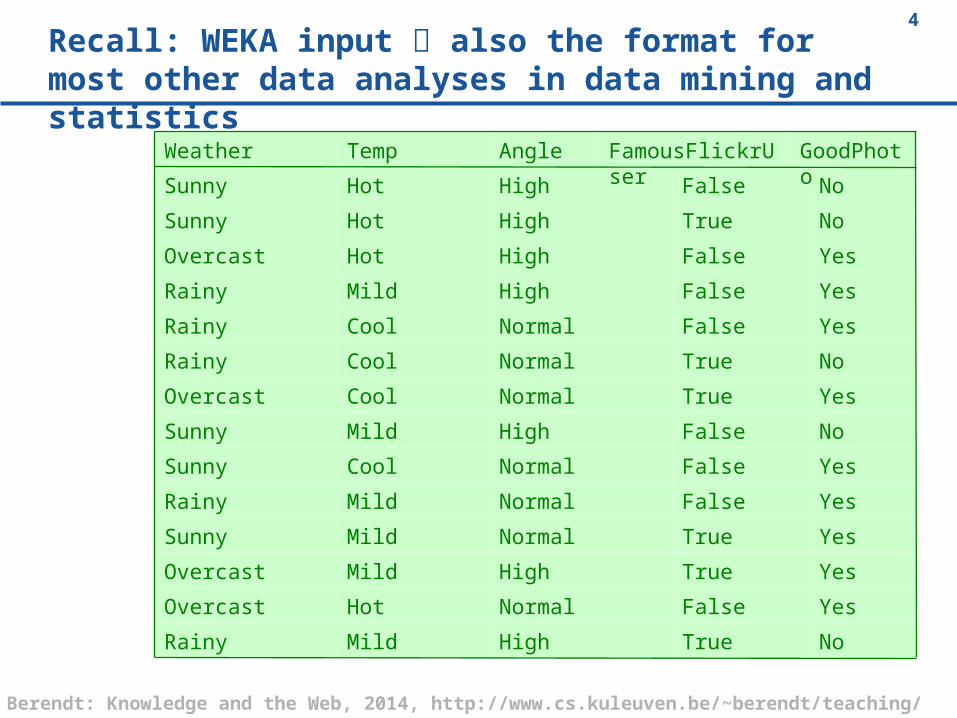
4Recall: WEKA input also the format for most other data analyses in data mining and statistics
NoTrueHighMildRainy
YesFalseNormalHotOvercast
YesTrueHighMildOvercast
YesTrueNormalMildSunny
YesFalseNormalMildRainy
YesFalseNormalCoolSunny
NoFalseHighMildSunny
YesTrueNormalCoolOvercast
NoTrueNormalCoolRainy
YesFalseNormalCoolRainy
YesFalseHighMildRainy
YesFalseHighHot Overcast
NoTrueHigh Hot Sunny
NoFalseHighHotSunny
GoodPhoto
FamousFlickrUser
AngleTempWeather
Berendt: Knowledge and the Web, 2014, http://www.cs.kuleuven.be/~berendt/teaching/
5
Propositionalization
Def.: The transformation of a relational dataset (a relational database, the individuals of an OWL ontology, ...) into one table
Should be relatively straightforward for your data.
But make sure you describe the resulting table and what the attributes mean clearly!
2 operations we expect you‘ll need to employ: Aggregation
– e.g. a set of userIDhasTakenphotoID triples into a triple userIDhasNumPhotosinteger
“Join“
– e.g. assembling all the information about any given userID (number of photos, of likes, ...) into one row in the table

Berendt: Knowledge and the Web, 2014, http://www.cs.kuleuven.be/~berendt/teaching/
6
Assume this is the result (our working example for today)
userID lat long numPhotos (in 1000s)1 0,01 0,81 58,42 0,4 0,4 51,63 0,17 0,99 59,24 0,17 0,07 58,25 1 0,64 536 0,62 0,77 57,97 0,86 0,27 59,58 0,44 0,36 52,59 0,44 0,04 56,5
10 0,34 0,17 57,511 0,46 1,28 62,212 0,79 1,26 67,113 0,03 1,39 63,514 0,41 1,13 61,815 0,39 1,36 61,916 0,38 1,74 64,617 0,05 1,3 61,8...
119 1,32 5,24 155,6
Berendt: Knowledge and the Web, 2014, http://www.cs.kuleuven.be/~berendt/teaching/
7
Agenda
Input: a table / propositionalization
Visual exploration and descriptive analysis
Hypothesis testing and data-mining evaluation
The chi-square test of independence
Hypotheses of difference of means: the t-test
Linear regression (in statistics, in WEKA)
Berendt: Knowledge and the Web, 2014, http://www.cs.kuleuven.be/~berendt/teaching/
8
Lead question
“How does one variable relate to another?“

Berendt: Knowledge and the Web, 2014, http://www.cs.kuleuven.be/~berendt/teaching/
9
Descriptive analysis: instances
0 1 2 3 4 5 6 70
20
40
60
80
100
120
140
160
180
numPhotos
numPhotos
0 1 2 3 4 5 6 70
10
20
30
40
50
60
70
80
90
Series1
0 1 2 3 4 5 6 70
20
40
60
80
100
120
140
160
180
Series1

Berendt: Knowledge and the Web, 2014, http://www.cs.kuleuven.be/~berendt/teaching/
10
Descriptive analysis: bins and bar charts
0 1 2 3 4 5 6 70
0.5
1
1.5
2
2.5
north
south
north/south west/east
numPhotosAgg
1 1 5421 2 651,71 3 7441 4 739,91 5 648,41 6 554,42 1 548,72 2 735,22 3 959,62 4 1149,12 5 1367,42 6 1537,9
Berendt: Knowledge and the Web, 2014, http://www.cs.kuleuven.be/~berendt/teaching/
11
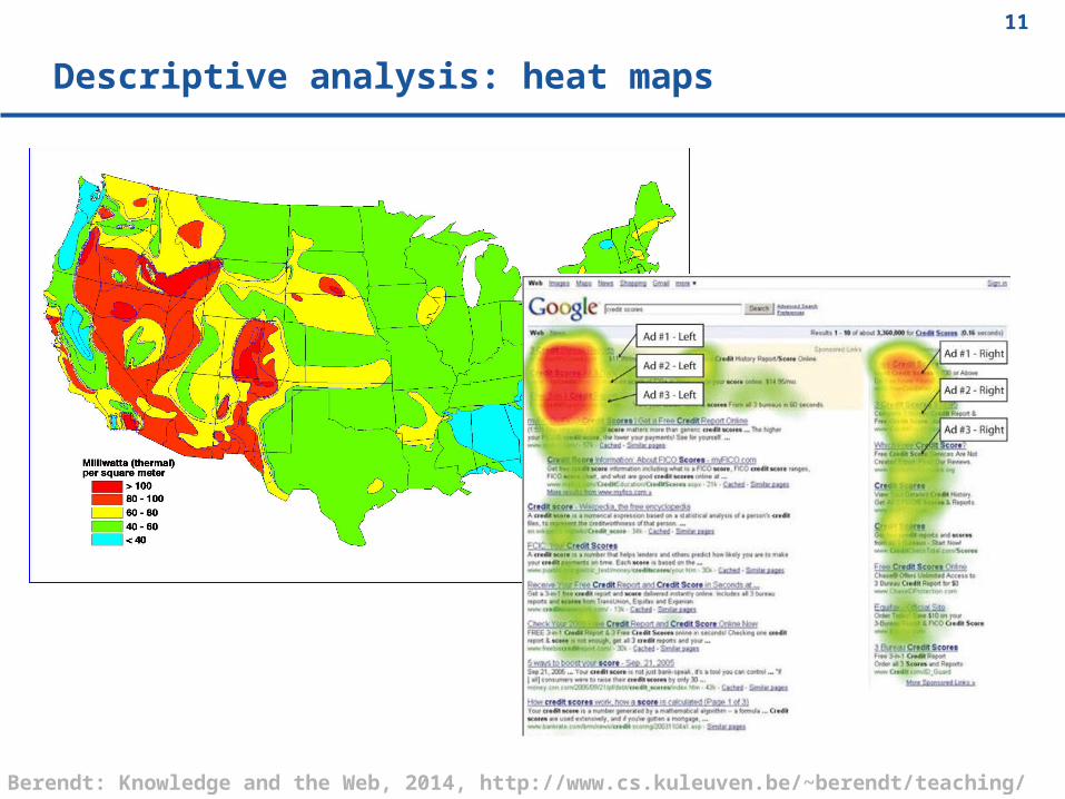
Descriptive analysis: heat maps

Berendt: Knowledge and the Web, 2014, http://www.cs.kuleuven.be/~berendt/teaching/
12
We think this may be relevant at least for projects ...
G (Amsterdam)
D – approach 1 (popularity)
Berendt: Knowledge and the Web, 2014, http://www.cs.kuleuven.be/~berendt/teaching/
13
Agenda
Input: a table / propositionalization
Visual exploration and descriptive analysis
Hypothesis testing and data-mining evaluation
The chi-square test of independence
Hypotheses of difference of means: the t-test
Linear regression (in statistics, in WEKA)
Berendt: Knowledge and the Web, 2014, http://www.cs.kuleuven.be/~berendt/teaching/
14
Hypothesis testing in a nutshell (1)
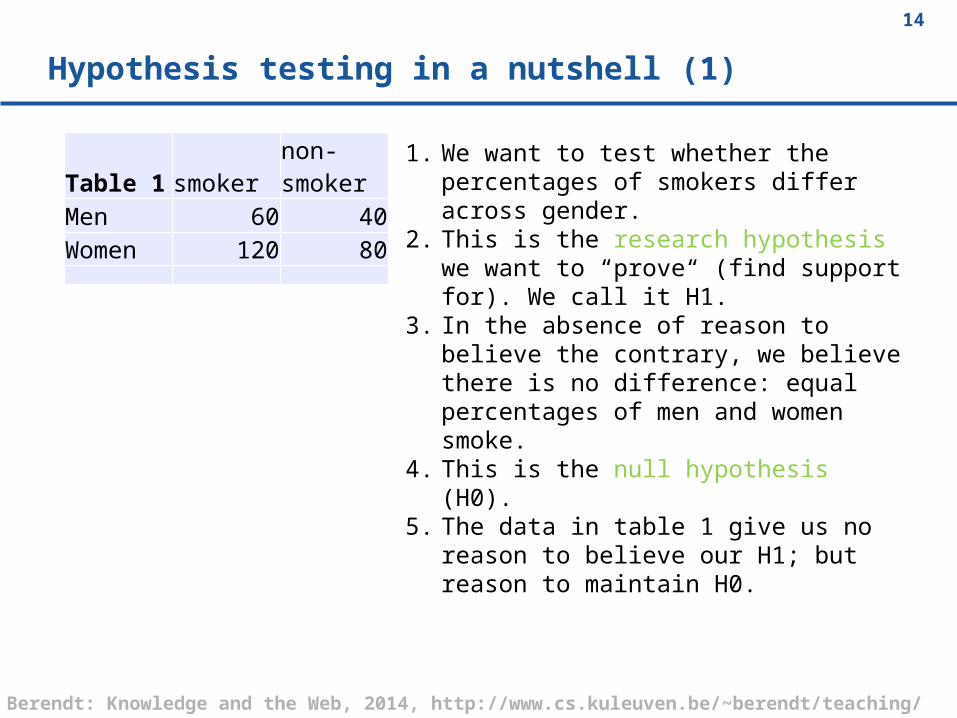
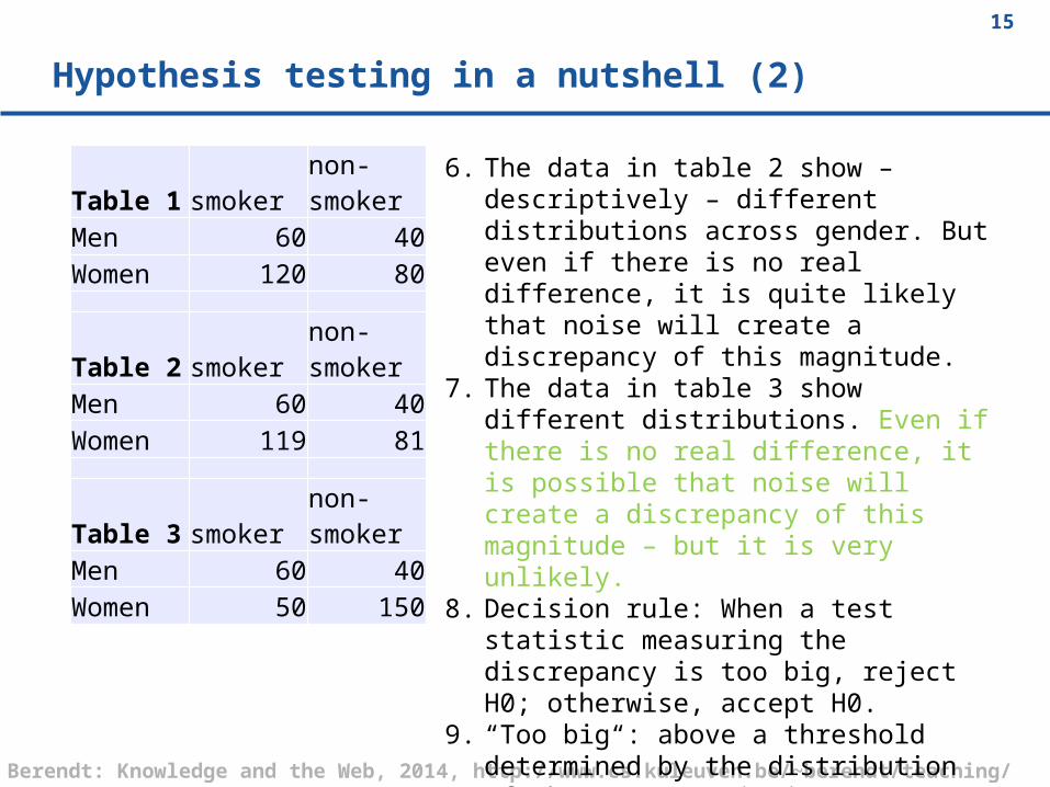
Table 1 smokernon-smoker
Men 60 40Women 120 80
1. We want to test whether the percentages of smokers differ across gender.
2. This is the research hypothesis we want to “prove“ (find support for). We call it H1.
3. In the absence of reason to believe the contrary, we believe there is no difference: equal percentages of men and women smoke.
4. This is the null hypothesis (H0).5. The data in table 1 give us no reason to
believe our H1; but reason to maintain H0.
Berendt: Knowledge and the Web, 2014, http://www.cs.kuleuven.be/~berendt/teaching/
15
Hypothesis testing in a nutshell (2)
Table 1 smokernon-smoker
Men 60 40Women 120 80
Table 2 smokernon-smoker
Men 60 40Women 119 81
Table 3 smokernon-smoker
Men 60 40Women 50 150
6. The data in table 2 show – descriptively – different distributions across gender. But even if there is no real difference, it is quite likely that noise will create a discrepancy of this magnitude.
7. The data in table 3 show different distributions. Even if there is no real difference, it is possible that noise will create a discrepancy of this magnitude – but it is very unlikely.
8. Decision rule: When a test statistic measuring the discrepancy is too big, reject H0; otherwise, accept H0.
9. “Too big“: above a threshold determined by the distribution of the test statistic.

Berendt: Knowledge and the Web, 2014, http://www.cs.kuleuven.be/~berendt/teaching/
16
Hypothesis testing in a nutshell (3)
Table 3 smokernon-smoker
Men 60 40Women 50 150
8. Decision rule: When a test statistic measuring the discrepancy is too big, reject H0; otherwise, accept H0.
9. “Too big“: above a threshold determined by the distribution of the test statistic.
10.Motivation: This makes it improbable to make a certain error.
11. Which error?12. “If there is no difference, the probability that
you would observe a discrepancy this big – or bigger – would be 5% (or 1%).“
13. In other words: restrict the probability of rejecting the H0 when H0 is true (~ erroneously believing the data support H1) .
14. It does not mean that the general error probability of your interpretation is low.
15. It also does not mean that “with 95% probability, H1 is true given our data“!

Berendt: Knowledge and the Web, 2014, http://www.cs.kuleuven.be/~berendt/teaching/
17
But data mining ...
... addresses this issue quite differently.
You can even get the same models (e.g. linear regression) in a statistics toolkit (such as SPSS or R *) and in a data-mining toolkit (such as WEKA), with rather different error reporting.
The reason is the entirely different emphasis/perspective on confirmatory analysis (where for hypothesis testing, data are
ideally specifically gathered, and then thrown away after one test has been administered) vs.
exploratory analysis (which looks at data repeatedly).
Note: There are also combinations of statistical and data-mining evaluation (often required in research reporting), and this is a contested topic, and really beyond the scope of this course!
* Mini-tutorial with data files on Toledo
Berendt: Knowledge and the Web, 2014, http://www.cs.kuleuven.be/~berendt/teaching/
18
Data mining model testing in a nutshell
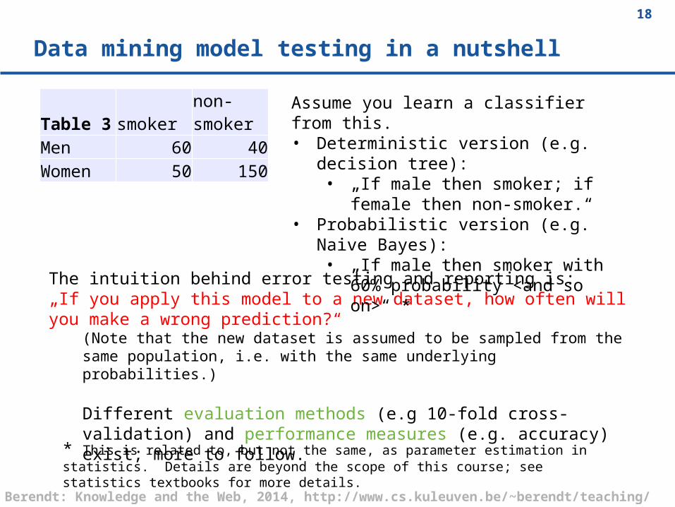
Table 3 smokernon-smoker
Men 60 40Women 50 150
The intuition behind error testing and reporting is:„If you apply this model to a new dataset, how often will you make a wrong prediction?“
(Note that the new dataset is assumed to be sampled from the same population, i.e. with the same underlying probabilities.)
Different evaluation methods (e.g 10-fold cross-validation) and performance measures (e.g. accuracy) exist; more to follow.
* This is related to, but not the same, as parameter estimation in statistics. Details are beyond the scope of this course; see statistics textbooks for more details.
Assume you learn a classifier from this.• Deterministic version (e.g. decision tree):
• „If male then smoker; if female then non-smoker.“
• Probabilistic version (e.g. Naive Bayes):• „If male then smoker with 60%
probability <and so on>“ *
Berendt: Knowledge and the Web, 2014, http://www.cs.kuleuven.be/~berendt/teaching/
19
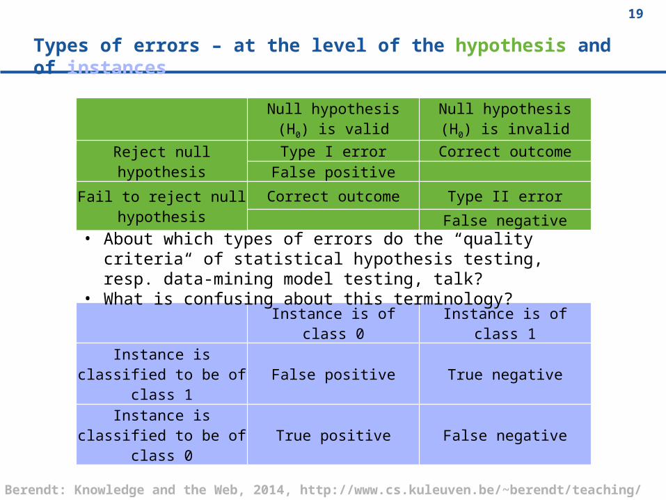
Types of errors – at the level of the hypothesis and of instances
Null hypothesis (H0) is valid
Null hypothesis (H0) is invalid
Reject null hypothesisType I error Correct outcome
False positive
Fail to reject null hypothesis
Correct outcome Type II error
False negative
Instance is of class 0 Instance is of class 1
Instance is classified to be of class 1 False positive True negative
Instance is classified to be of class 0 True positive False negative
• About which types of errors do the “quality criteria“ of statistical hypothesis testing, resp. data-mining model testing, talk?
• What is confusing about this terminology?
Berendt: Knowledge and the Web, 2014, http://www.cs.kuleuven.be/~berendt/teaching/
20
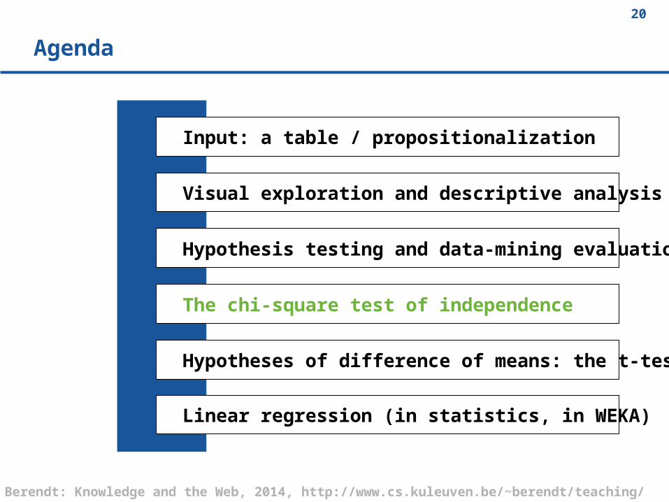
Agenda
Input: a table / propositionalization
Visual exploration and descriptive analysis
Hypothesis testing and data-mining evaluation
The chi-square test of independence
Hypotheses of difference of means: the t-test
Linear regression (in statistics, in WEKA)
Berendt: Knowledge and the Web, 2014, http://www.cs.kuleuven.be/~berendt/teaching/
21
Parametric and Nonparametric Tests
The term "non-parametric" refers to the fact that the chi‑square tests do not require assumptions about population parameters nor do they test hypotheses about population parameters.
Other examples of hypothesis tests (not covered in this lecture), such as the t tests and analysis of variance, are parametric tests and they do include assumptions about parameters and hypotheses about parameters. Slides 16-24: slightly adapted from https://home.ubalt.edu/tmitch/631/PowerPoint_Lectures/chapter18/chapter18.ppt

Berendt: Knowledge and the Web, 2014, http://www.cs.kuleuven.be/~berendt/teaching/
22
22
Data
The most obvious difference between the chi‑square tests and the other hypothesis tests (t and ANOVA) is the nature of the data.
For chi‑square, the data are frequencies rather than numerical scores.
Berendt: Knowledge and the Web, 2014, http://www.cs.kuleuven.be/~berendt/teaching/
23
23
The Chi-Square Test for Independence
This views the data as two (or more) separate samples representing the different populations being compared.*
The same variable is measured for each sample by classifying individual subjects into categories of the variable.
The data are presented in a matrix with the different samples defining the rows and the categories of the variable defining the columns.
* For a 2nd version, see linked slideset.
Berendt: Knowledge and the Web, 2014, http://www.cs.kuleuven.be/~berendt/teaching/
24
24
The Chi-Square Test for Independence (cont.)
The data, called observed frequencies, show how many individuals are in each cell of the matrix.
The null hypothesis for this test states that the proportions (the distribution across categories) are the same for all of the populations.
Berendt: Knowledge and the Web, 2014, http://www.cs.kuleuven.be/~berendt/teaching/
25
25
The Chi-Square Test for Independence (cont.)
Both* chi-square tests use the same statistic. The calculation of the chi-square statistic requires two steps:
1. The null hypothesis is used to construct an idealized sample distribution of expected frequencies that describes how the sample would look if the data were in perfect agreement with the null hypothesis.
* See hyperlinked slideset for details.
Berendt: Knowledge and the Web, 2014, http://www.cs.kuleuven.be/~berendt/teaching/
26
26
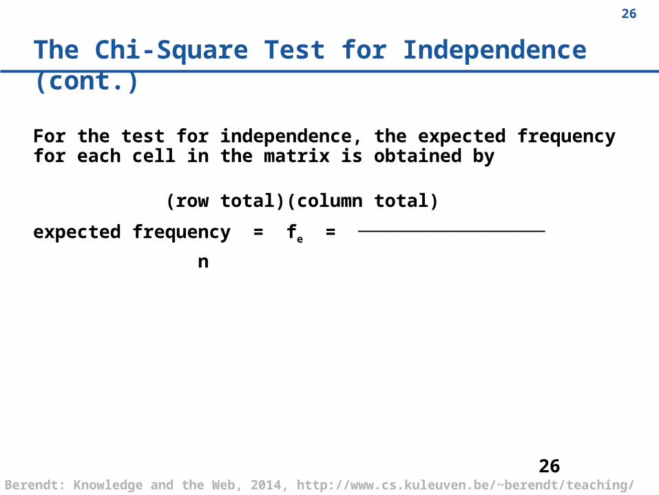
The Chi-Square Test for Independence (cont.)
For the test for independence, the expected frequency for each cell in the matrix is obtained by
(row total)(column total)
expected frequency = fe = ─────────────────
n
Berendt: Knowledge and the Web, 2014, http://www.cs.kuleuven.be/~berendt/teaching/
27
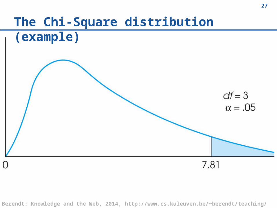
The Chi-Square distribution (example)
Berendt: Knowledge and the Web, 2014, http://www.cs.kuleuven.be/~berendt/teaching/
28
28
The Chi-Square Test for Independence (cont.)
2. A chi-square statistic is computed to measure the amount of discrepancy between the ideal sample (expected frequencies from H0) and the actual sample data (the observed frequencies = fo).
A large discrepancy results in a large value for chi-square and indicates that the data do not fit the null hypothesis and the hypothesis should be rejected.

Berendt: Knowledge and the Web, 2014, http://www.cs.kuleuven.be/~berendt/teaching/
29
29
The Chi-Square Test for Independence (cont.)
The calculation of chi-square is the same for all chi-square tests:
(fo – fe)2
chi-square = χ2 = Σ ─────
fe
The fact that chi‑square tests do not require scores from an interval or ratio scale makes these tests a valuable alternative to the t tests, ANOVA, or correlation, because they can be used with data measured on a nominal or an ordinal scale.
Berendt: Knowledge and the Web, 2014, http://www.cs.kuleuven.be/~berendt/teaching/
30
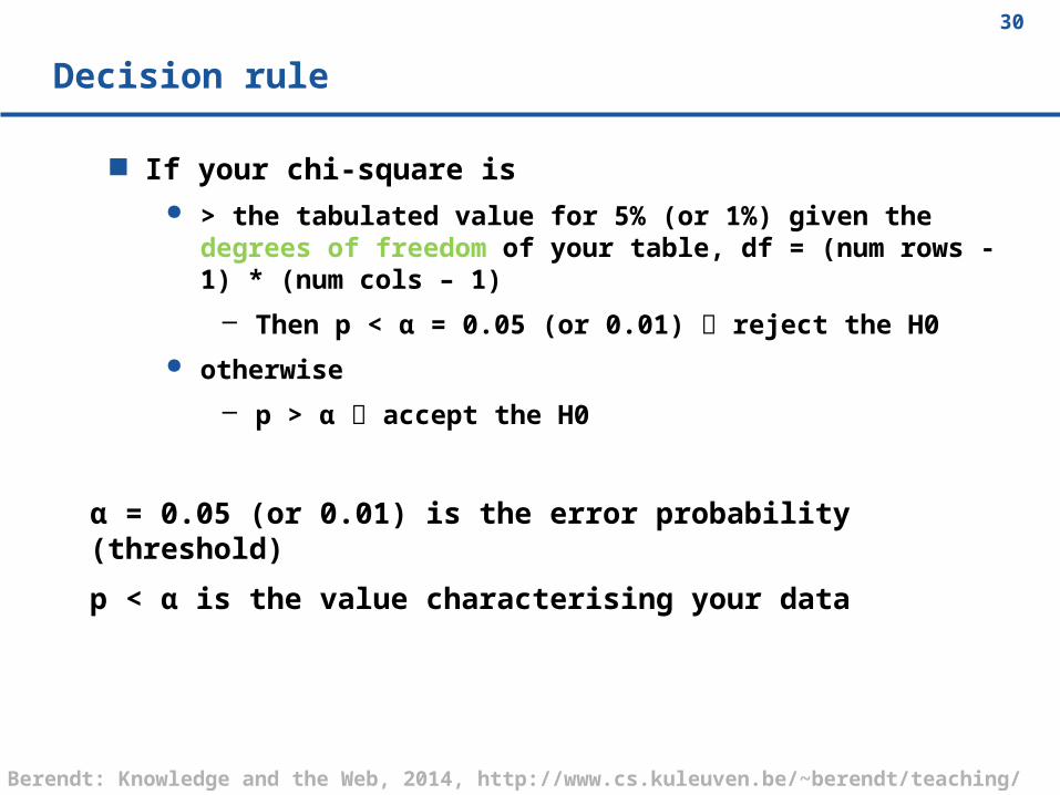
Decision rule
If your chi-square is > the tabulated value for 5% (or 1%) given the degrees of
freedom of your table, df = (num rows -1) * (num cols – 1)
– Then p < α = 0.05 (or 0.01) reject the H0
otherwise
– p > α accept the H0
α = 0.05 (or 0.01) is the error probability (threshold)
p < α is the value characterising your data
Berendt: Knowledge and the Web, 2014, http://www.cs.kuleuven.be/~berendt/teaching/
31
Where do I find the tabulated values?
e.g.
http://www.medcalc.org/manual/chi-square-table.php
Berendt: Knowledge and the Web, 2014, http://www.cs.kuleuven.be/~berendt/teaching/
32
We think this may be relevant at least for projects ...
D – approach 2 (popularity)
Berendt: Knowledge and the Web, 2014, http://www.cs.kuleuven.be/~berendt/teaching/
33
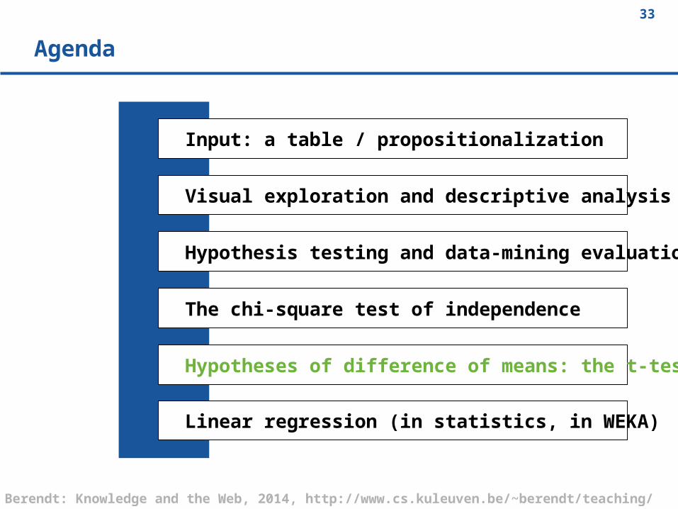
Agenda
Input: a table / propositionalization
Visual exploration and descriptive analysis
Hypothesis testing and data-mining evaluation
The chi-square test of independence
Hypotheses of difference of means: the t-test
Linear regression (in statistics, in WEKA)
Berendt: Knowledge and the Web, 2014, http://www.cs.kuleuven.be/~berendt/teaching/
34
Lead question
“Does one variable affect the value of the other?“
Here: the t-test for independent samples

Berendt: Knowledge and the Web, 2014, http://www.cs.kuleuven.be/~berendt/teaching/
35
35
Independent-Measures Designs
The independent-measures hypothesis test allows researchers to evaluate the mean difference between two populations using the data from two separate samples.
The identifying characteristic of the independent-measures or between-subjects design is the existence of two separate or independent samples.
Thus, an independent-measures design can be used to test for mean differences between two distinct populations (such as men versus women) or between two different treatment conditions (such as drug versus no-drug).
Slides 31-39: slightly adapted from https://home.ubalt.edu/tmitch/631/PowerPoint_Lectures/chapter10/chapter10.ppt

Berendt: Knowledge and the Web, 2014, http://www.cs.kuleuven.be/~berendt/teaching/
36
Berendt: Knowledge and the Web, 2014, http://www.cs.kuleuven.be/~berendt/teaching/
37
37
Independent-Measures Designs (cont.)
The independent-measures design is used in situations where a researcher has no prior knowledge about either of the two populations (or treatments) being compared.
In particular, the population means and standard deviations are all unknown.
Because the population variances are not known, these values must be estimated from the sample data.
Berendt: Knowledge and the Web, 2014, http://www.cs.kuleuven.be/~berendt/teaching/
38
38
Hypothesis Testing with the Independent-Measures t Statistic
As with all hypothesis tests, the general purpose of the independent-measures t test is to determine whether the sample mean difference obtained in a research study indicates a real mean difference between the two populations (or treatments) or whether the obtained difference is simply the result of sampling error.
Remember, if two samples are taken from the same population and are given exactly the same treatment, there still will be some difference between the sample means.
Berendt: Knowledge and the Web, 2014, http://www.cs.kuleuven.be/~berendt/teaching/
39
39
Hypothesis Testing with the Independent-Measures t Statistic (cont.)
This difference is called sampling error
The hypothesis test provides a standardized, formal procedure for determining whether the mean difference obtained in a research study is significantly greater than can be explained by sampling error
Berendt: Knowledge and the Web, 2014, http://www.cs.kuleuven.be/~berendt/teaching/
40
40
Hypothesis Testing with the Independent-Measures t Statistic (cont.)
To prepare the data for analysis, the first step is to compute the sample mean and SS (or s, or s2) for each of the two samples.
The hypothesis test follows the same four-step procedure outlined in Chapters 8 and 9.
Berendt: Knowledge and the Web, 2014, http://www.cs.kuleuven.be/~berendt/teaching/
41
41
Hypothesis Testing with the Independent-Measures t Statistic (cont.)
1. State the hypotheses and select an α level. For the independent-measures test, H0 states that there is no difference between the two population means.
2. Locate the critical region. The critical values for the t statistic are obtained using degrees of freedom that are determined by adding together the df value for the first sample and the df value for the second sample.
Berendt: Knowledge and the Web, 2014, http://www.cs.kuleuven.be/~berendt/teaching/
42
42
Hypothesis Testing with the Independent-Measures t Statistic (cont.)
3. Compute the test statistic. The t statistic for the independent-measures design has the same structure as the single sample t introduced in Chapter 9. However, in the independent-measures situation, all components of the t formula are doubled: there are two sample means, two population means, and two sources of error contributing to the standard error in the denominator.
4. Make a decision. If the t statistic ratio indicates that the obtained difference between sample means (numerator) is substantially greater than the difference expected by chance (denominator), we reject H0 and conclude that there is a real mean difference between the two populations or treatments.

Berendt: Knowledge and the Web, 2014, http://www.cs.kuleuven.be/~berendt/teaching/
43
Berendt: Knowledge and the Web, 2014, http://www.cs.kuleuven.be/~berendt/teaching/
44
Where do I find the tabulated values?
e.g.
https://www.easycalculation.com/statistics/t-distribution-critical-value-table.php
Berendt: Knowledge and the Web, 2014, http://www.cs.kuleuven.be/~berendt/teaching/
45
We think this may be relevant at least for projects ...
D – approach 2 (popularity)
E (weather)

Berendt: Knowledge and the Web, 2014, http://www.cs.kuleuven.be/~berendt/teaching/
46
Agenda
Input: a table / propositionalization
Visual exploration and descriptive analysis
Hypothesis testing and data-mining evaluation
The chi-square test of independence
Hypotheses of difference of means: the t-test
Linear regression (in statistics, in WEKA)
Berendt: Knowledge and the Web, 2014, http://www.cs.kuleuven.be/~berendt/teaching/
47
Lead question
“How does the dependent variable depend on the independent one?“
“Can we predict the likely value of the dependent variable for a new data instance (with a given value of the independent variable)?“

Berendt: Knowledge and the Web, 2014, http://www.cs.kuleuven.be/~berendt/teaching/
48
48
Introduction to Linear Regression(the statistical approach)
The Pearson correlation measures the degree to which a set of data points form a straight line relationship.
Regression is a statistical procedure that determines the equation for the straight line that best fits a specific set of data.
Slides 44-49: slightly adapted from https://home.ubalt.edu/tmitch/631/PowerPoint_Lectures/chapter17/chapter17.ppt

Berendt: Knowledge and the Web, 2014, http://www.cs.kuleuven.be/~berendt/teaching/
49
49
Introduction to Linear Regression (cont.)
Any straight line can be represented by an equation of the form Y = bX + a, where b and a are constants.
The value of b is called the slope constant and determines the direction and degree to which the line is tilted.
The value of a is called the Y-intercept and determines the point where the line crosses the Y-axis.

Berendt: Knowledge and the Web, 2014, http://www.cs.kuleuven.be/~berendt/teaching/
50
Berendt: Knowledge and the Web, 2014, http://www.cs.kuleuven.be/~berendt/teaching/
51
51
Introduction to Linear Regression (cont.)
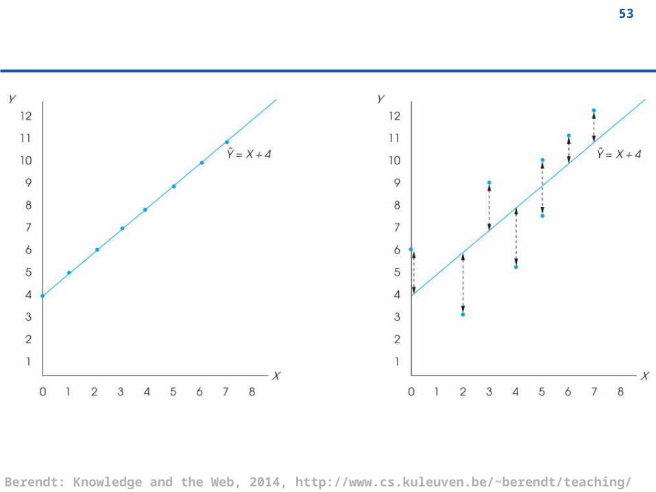
How well a set of data points fits a straight line can be measured by calculating the distance between the data points and the line.
The total error between the data points and the line is obtained by squaring each distance and then summing the squared values.
The regression equation is designed to produce the minimum sum of squared errors.
Berendt: Knowledge and the Web, 2014, http://www.cs.kuleuven.be/~berendt/teaching/
52
52
Introduction to Linear Regression (cont.)
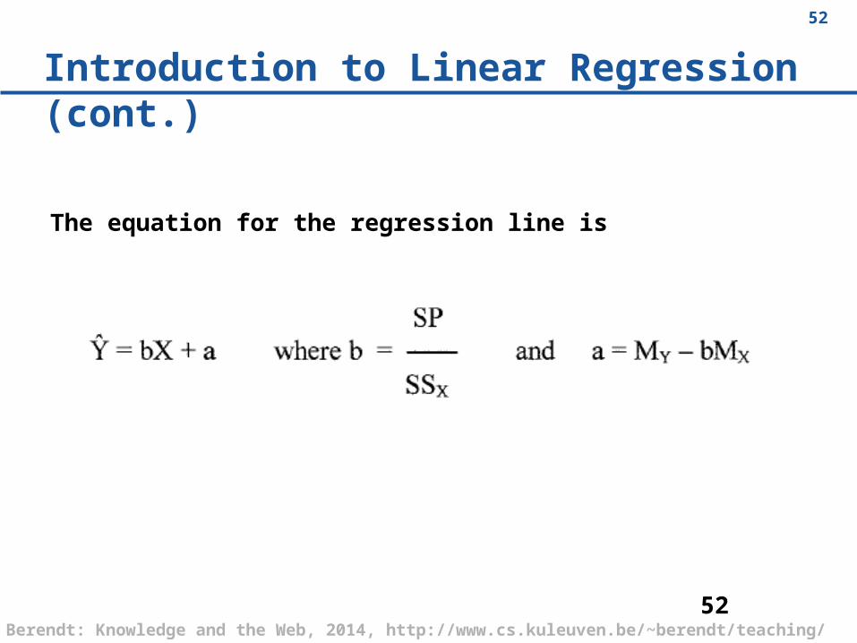
The equation for the regression line is
Berendt: Knowledge and the Web, 2014, http://www.cs.kuleuven.be/~berendt/teaching/
53

Berendt: Knowledge and the Web, 2014, http://www.cs.kuleuven.be/~berendt/teaching/
54
And now for the data-mining / WEKA approach

Berendt: Knowledge and the Web, 2014, http://www.cs.kuleuven.be/~berendt/teaching/
55
Numeric prediction
Variant of classification learning where “class” is numeric (also called “regression”)
Learning is supervised Scheme is being provided with target
value Measure success on test data
……………
40FalseNormalMildRainy
55FalseHighHot Overcast
0TrueHigh Hot Sunny
5FalseHighHotSunny
Play-timeWindyHumidityTemperatureOutlook
Berendt: Knowledge and the Web, 2014, http://www.cs.kuleuven.be/~berendt/teaching/
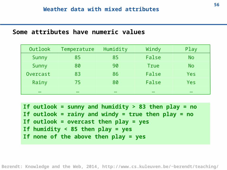
56Weather data with mixed attributes
Some attributes have numeric values
……………
YesFalse8075Rainy
YesFalse8683Overcast
NoTrue9080Sunny
NoFalse8585Sunny
PlayWindyHumidityTemperatureOutlook
If outlook = sunny and humidity > 83 then play = noIf outlook = rainy and windy = true then play = noIf outlook = overcast then play = yesIf humidity < 85 then play = yesIf none of the above then play = yes
Berendt: Knowledge and the Web, 2014, http://www.cs.kuleuven.be/~berendt/teaching/
57
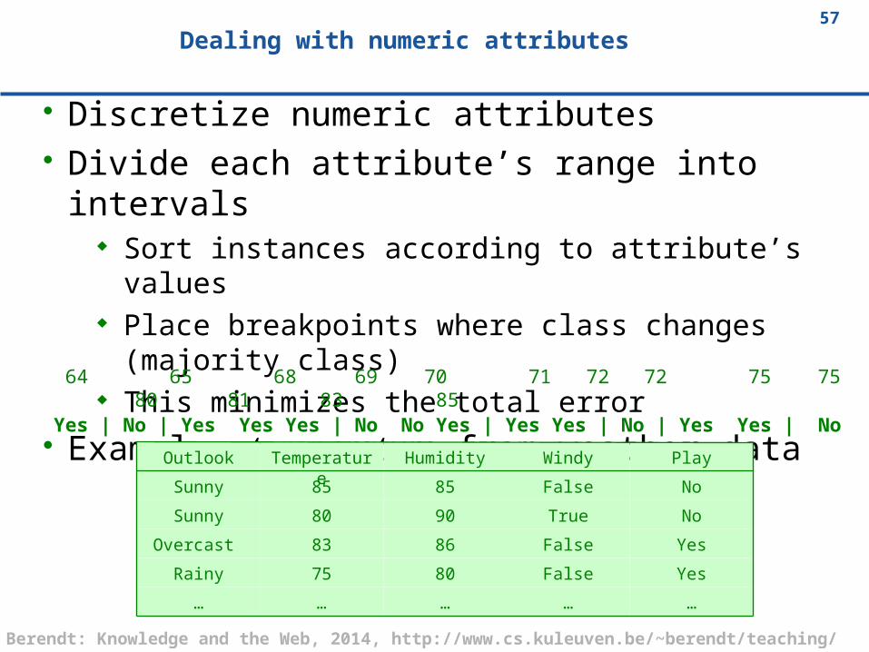
Dealing with numeric attributes
Discretize numeric attributes Divide each attribute’s range into intervals
Sort instances according to attribute’s values Place breakpoints where class changes (majority
class) This minimizes the total error
Example: temperature from weather data 64 65 68 69 70 71 72 72 75 75 80 81 83 85Yes | No | Yes Yes Yes | No No Yes | Yes Yes | No | Yes Yes | No
……………
YesFalse8075Rainy
YesFalse8683Overcast
NoTrue9080Sunny
NoFalse8585Sunny
PlayWindyHumidityTemperature
Outlook
Berendt: Knowledge and the Web, 2014, http://www.cs.kuleuven.be/~berendt/teaching/
58
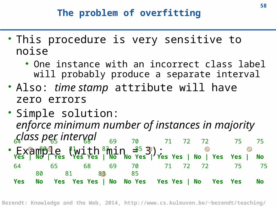
The problem of overfitting
This procedure is very sensitive to noise One instance with an incorrect class label will
probably produce a separate interval Also: time stamp attribute will have zero
errors Simple solution:
enforce minimum number of instances in majority class per interval
Example (with min = 3):64 65 68 69 70 71 72 72 75 75 80 81 83 85Yes | No | Yes Yes Yes | No No Yes | Yes Yes | No | Yes Yes | No
64 65 68 69 70 71 72 72 75 75 80 81 83 85Yes No Yes Yes Yes | No No Yes Yes Yes | No Yes Yes No

Berendt: Knowledge and the Web, 2014, http://www.cs.kuleuven.be/~berendt/teaching/
59
Nominal and numeric attributes
Nominal:number of children usually equal to number values attribute won’t get tested more than once Other possibility: division into two subsets
Numeric:test whether value is greater or less than constant attribute may get tested several times Other possibility: three-way split (or multi-way split)
Integer: less than, equal to, greater than Real: below, within, above
Berendt: Knowledge and the Web, 2014, http://www.cs.kuleuven.be/~berendt/teaching/
60
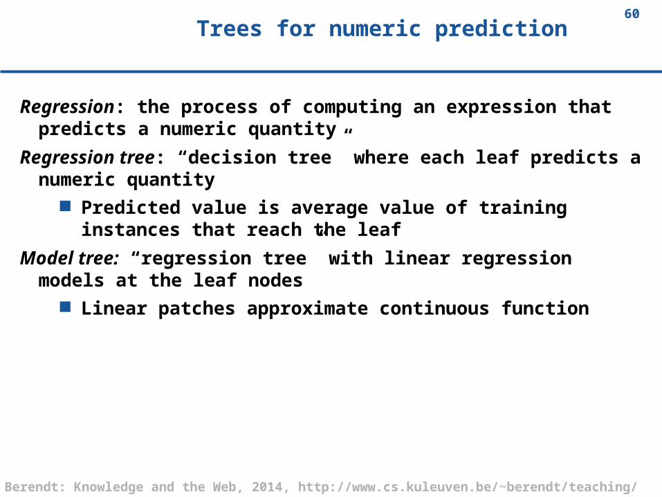
Trees for numeric prediction
Regression: the process of computing an expression that predicts a numeric quantity
Regression tree: “decision tree” where each leaf predicts a numeric quantity
Predicted value is average value of training instances that reach the leaf
Model tree: “regression tree” with linear regression models at the leaf nodes
Linear patches approximate continuous function
Berendt: Knowledge and the Web, 2014, http://www.cs.kuleuven.be/~berendt/teaching/
61
WEKA also supports standard linear regression!
62Data Mining: Practical Machine Learning Tools and Techniques (Chapter 5)
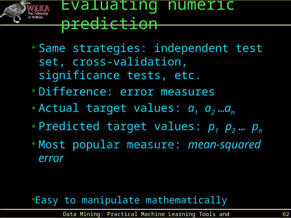
Evaluating numeric prediction
● Same strategies: independent test set, cross-validation, significance tests, etc.
● Difference: error measures● Actual target values: a1 a2 …an
● Predicted target values: p1 p2 … pn
● Most popular measure: mean-squared error
●Easy to manipulate mathematically
(𝑝1−𝑎1 )2+ ...+(𝑝𝑛−𝑎𝑛)2
𝑛

63Data Mining: Practical Machine Learning Tools and Techniques (Chapter 5)
Other measures● The root mean-squared error :
● The mean absolute error is less sensitive to outliers than the mean-squared error:
● Sometimes relative error values are more appropriate (e.g. 10% for an error of 50 when predicting 500)
√ (𝑝1−𝑎1 )2+ ...+(𝑝𝑛−𝑎𝑛)2
𝑛
∣𝑝1−𝑎1 ∣+...+ ∣𝑝𝑛−𝑎𝑛 ∣𝑛

64Data Mining: Practical Machine Learning Tools and Techniques (Chapter 5)
Improvement on the mean
● How much does the scheme improve on simply predicting the average?
● The relative squared error is:
● The relative absolute error is:
𝑝1−𝑎12 ... 𝑝𝑛−𝑎𝑛
2
𝑎
−𝑎12 ... 𝑎
−𝑎𝑛2
∣𝑝1−𝑎1 ∣ ... ∣𝑝𝑛−𝑎𝑛 ∣
∣ 𝑎
−𝑎1∣ ... ∣𝑎
−𝑎𝑛∣

65Data Mining: Practical Machine Learning Tools and Techniques (Chapter 5)
Correlation coefficient
● Measures the statistical correlation between the predicted values and the actual values
● Scale independent, between –1 and +1● Good performance leads to large values!

66Data Mining: Practical Machine Learning Tools and Techniques (Chapter 5)
Which measure?
● Best to look at all of them● Often it doesn’t matter● Example:
0.910.890.880.88Correlation coefficient
30.4%34.8%40.1%43.1%Relative absolute error
35.8%39.4%57.2%42.2%Root rel squared error
29.233.438.541.3Mean absolute error
57.463.391.767.8Root mean-squared error
DCBA
● D best● C second-
best● A, B
arguable

Berendt: Knowledge and the Web, 2014, http://www.cs.kuleuven.be/~berendt/teaching/
67
We think this may be relevant at least for projects ...
A (pubgoers)
C (restaurants)
H (popular routes)
Berendt: Knowledge and the Web, 2014, http://www.cs.kuleuven.be/~berendt/teaching/
68
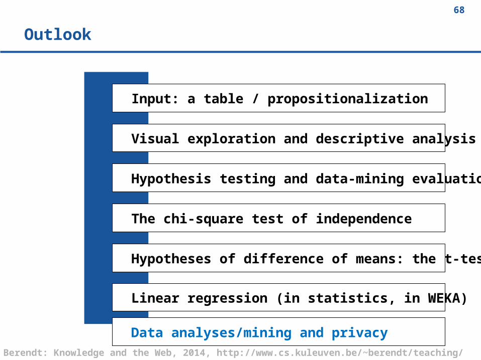
Outlook
Input: a table / propositionalization
Visual exploration and descriptive analysis
Hypothesis testing and data-mining evaluation
The chi-square test of independence
Hypotheses of difference of means: the t-test
Linear regression (in statistics, in WEKA)
Data analyses/mining and privacy
Berendt: Knowledge and the Web, 2014, http://www.cs.kuleuven.be/~berendt/teaching/
69
References / background reading; acknowledgements
The data mining slides are based on / taken from the instructor slides of Witten, I.H., & Frank, E.(2011). Data Mining. Practical Machine Learning Tools and
Techniques with Java Implementations. 3rd ed. Morgan Kaufmann. http://www.cs.waikato.ac.nz/ml/weka/book.html
Recommended reading: the book
Technical details on the other techniques can be found in any standard statistics textbook – consult your local library.
Many thanks to Tom Mitchell for his statistics slides (hyperlinked in this PPT)!