Embed Size (px)
Citation preview

Bennie D Waller, Longwood University
Probability

Bennie D Waller, Longwood University
Probability Probability - the likelihood of an
event occurring
0<=P(X)<=1

Bennie D Waller, Longwood University
Probability
Classical Probability –flipping a coin
Empirical Probability – based on prior events – airline arrival
Subjective Probability – Longwood baseball winning CWS

Bennie D Waller, Longwood University
Probability
Marginal Probability – the likelihood of a particular event occurring P(Smoker)
Joint Probability – the likelihood of two events both occurring – P(Male AND Smoker)
Conditional Probability – likelihood of an event occurring based the previous outcome of another event – P(Rain | Cloudy)
Independence – two events are independent if one’s outcome does not impact the other’s outcome
Mutually exclusive – if one event occurs, the other cannot

Bennie D Waller, Longwood University
Probability
P(A or B) = P(A) + P(B) - P(A and B)
P(A or B) = P(A) + P(B)
Rules of addition

Bennie D Waller, Longwood University
P(A and B) = P(A)P(B|A)
P(A and B) = P(A)P(B)
Probability
Rules of multiplication

Bennie D Waller, Longwood University
Contingency Tables
.30 .05
.20 .45
Male Female
Smoker
Non-smoker
.50 .50
.35
.65

Bennie D Waller, Longwood University
ExamplesProblem: A student is taking two courses, history and math. The probability that the student will pass the history class is .60 and the probability of passing the math class is .70. The probability of passing both is .50. What is the probability of passing at least one of the classes?

Bennie D Waller, Longwood University
Problem: A study by the National Park Service revealed that 50% of the vacationers going to the Rocky Mountain region visit Yellowstone Park, 40% visit the Tetons and 35% visit both. 1. What is the probability that a vacationer will visit at least one of these magnificent
attractions? 2. What is the .35 probability called? 3. Are these events mutually exclusive?
.50 .40.35

Bennie D Waller, Longwood University
General Multiplication Rule
A golfer has 12 golf shirts in his closet. Suppose 9 of these shirts are white and the others blue. He gets dressed in the dark, so he just grabs a shirt and puts it on. He plays golf two days in a row and does not do laundry.
What is the likelihood both shirts selected are white?
P(A and B) = P(A)*P(B|A)

Bennie D Waller, Longwood University
Contingency Tables
In a survey of employee satisfaction, the following table summarizes the results in terms of employee satisfaction and gender.
1. What is the probability that an employee is Female and Dissatisfied?2. What is the probability that an employee is Male or Dissatisfied? 3. What is the probability that an employee is Satisfied given that the employee is Male?

Bennie D Waller, Longwood University
Problem: Airlines monitor the causes of flights arriving late. 75% of flights are late because of weather, 35% of flights are late because of ground operations. 15% of flights are late because of weather and ground operations. What is the probability that a flight arrives late because of weather or ground operations?

Bennie D Waller, Longwood University
Discrete Probability
Bennie Waller
434-395-2046Longwood University
201 High StreetFarmville, VA 23901

Bennie D Waller, Longwood University
Discrete Probability Distributions
DISCRETE RANDOM VARIABLE - A variable that can assume only certain clearly separated values and is the typically the result of counting something.
CHARACTERISTICS OF A PROBABILITY DISTRIBUTION
1.The probability of a particular outcome is between 0 and 1 inclusive.
2. The outcomes are mutually exclusive events.
3. The list is exhaustive. So the sum of the probabilities of the various events is equal to 1.
CONTINUOUS RANDOM VARIABLE – A variable that can assume an infinite number of values within a given range. It is usually the result of some type of measurement

Bennie D Waller, Longwood University
Experiment:
Toss a coin three times. Observe the number of heads. The possible results are: Zero heads, One head, Two heads, andThree heads.
What is the probability distribution for the number of heads?
PROBABILITY DISTRIBUTION A listing of all the outcomes of an experiment and the probability associated with each outcome.
6-15
Probability Distributions

Bennie D Waller, Longwood University
Discrete Probability Distribution
Mean
X P(x)
.05 .20
.06 .20
.07 .20
.08 .20
.09 .20

Bennie D Waller, Longwood University
Discrete Probability Distribution
Variance
X P(x)
.05 .20
.06 .20
.07 .20
.08 .20
.09 .20
Bennie D Waller, Longwood University
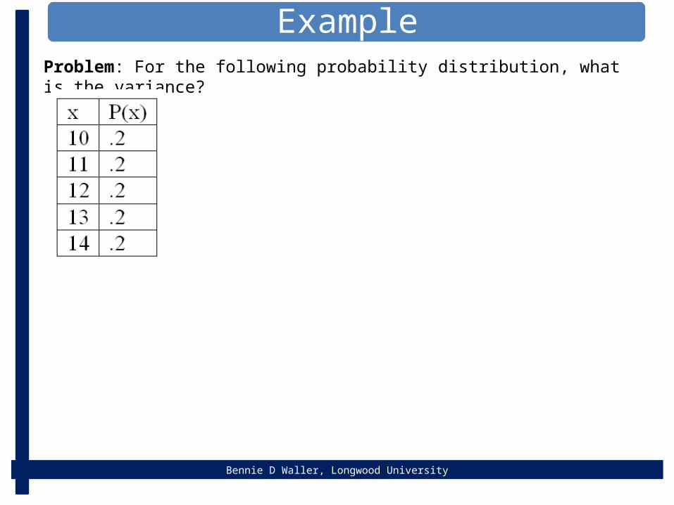
Example
Problem: For the following probability distribution, what is the variance?

Bennie D Waller, Longwood University
Continuous Probability
Bennie Waller
434-395-2046Longwood University
201 High StreetFarmville, VA 23901

Bennie D Waller, Longwood University
Characteristics of a Normal Probability Distribution
1. It is bell-shaped.
2. It is symmetrical about the mean
3. It is asymptotic:
4. The location of a normal distribution is determined by the mean,, the dispersion is determined by the standard deviation,σ .
5. The arithmetic mean, median, and mode are equal
6. The total area under the curve is 1.00; half the area under the normal curve is to the right of this center point, the mean, and the other half to the left of it.
7-20
Continuous Distributions

Bennie D Waller, Longwood University
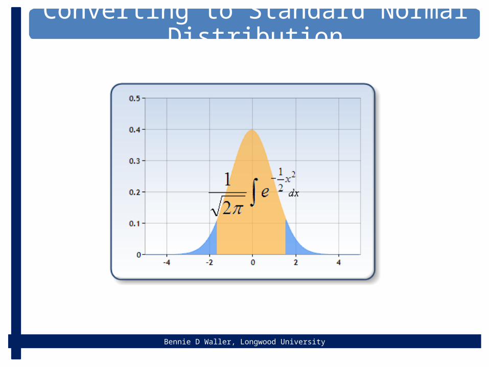
Converting to Standard Normal Distribution
Bennie D Waller, Longwood University
Converting to Standard Normal Distribution

Bennie D Waller, Longwood University
The Standard Normal Probability Distribution
• The standard normal distribution is a normal distribution with a mean of 0 and a standard deviation of 1.
• It is also called the z distribution. • A z-value is the signed distance between a selected
value, designated X, and the population mean , divided by the population standard deviation, σ.
• The formula is:
7-23
Converting to Standard Normal Distribution

Bennie D Waller, Longwood University
Standard Normal DistributionTables
z 0.00 0.01 0.02 0.03 0.04 0.05 0.06 0.07 0.08 0.09
0.0 0.0000 0.0040 0.0080 0.0120 0.0160 0.0190 0.0239 0.0279 0.0319 0.0359
0.1 0.0398 0.0438 0.0478 0.0517 0.0557 0.0596 0.0636 0.0675 0.0714 0.0753
0.2 0.0793 0.0832 0.0871 0.0910 0.0948 0.0987 0.1026 0.1064 0.1103 0.1141
0.3 0.1179 0.1217 0.1255 0.1293 0.1331 0.1368 0.1406 0.1443 0.1480 0.1517
0.4 0.1554 0.1591 0.1628 0.1664 0.1700 0.1736 0.1772 0.1808 0.1844 0.1879
0.5 0.1915 0.1950 0.1985 0.2019 0.2054 0.2088 0.2123 0.2157 0.2190 0.2224
0.6 0.2257 0.2291 0.2324 0.2357 0.2389 0.2422 0.2454 0.2486 0.2517 0.2549
0.7 0.2580 0.2611 0.2642 0.2673 0.2704 0.2734 0.2764 0.2794 0.2823 0.2852
0.8 0.2881 0.2910 0.2939 0.2969 0.2995 0.3023 0.3051 0.3078 0.3106 0.3133
0.9 0.3159 0.3186 0.3212 0.3238 0.3264 0.3289 0.3315 0.3340 0.3365 0.3389
1.0 0.3413 0.3438 0.3461 0.3485 0.3508 0.3513 0.3554 0.3577 0.3529 0.3621
1.1 0.3643 0.3665 0.3686 0.3708 0.3729 0.3749 0.3770 0.3790 0.3810 0.3830
1.2 0.3849 0.3869 0.3888 0.3907 0.3925 0.3944 0.3962 0.3980 0.3997 0.4015
1.3 0.4032 0.4049 0.4066 0.4082 0.4099 0.4115 0.4131 0.4147 0.4162 0.4177
1.4 0.4192 0.4207 0.4222 0.4236 0.4251 0.4265 0.4279 0.4292 0.4306 0.4319
1.5 0.4332 0.4345 0.4357 0.4370 0.4382 0.4394 0.4406 0.4418 0.4429 0.4441
1.6 0.4452 0.4463 0.4474 0.4484 0.4495 0.4505 0.4515 0.4525 0.4535 0.4545
1.7 0.4554 0.4564 0.4573 0.4582 0.4591 0.4599 0.4608 0.4616 0.4625 0.4633
1.8 0.4641 0.4649 0.4656 0.4664 0.4671 0.4678 0.4686 0.4693 0.4699 0.4706
1.9 0.4713 0.4719 0.4726 0.4732 0.4738 0.4744 0.4750 0.4756 0.4761 0.4767
2.0 0.4772 0.4778 0.4783 0.4788 0.4793 0.4798 0.4803 0.4808 0.4812 0.4817
2.1 0.4821 0.4826 0.4830 0.4834 0.4838 0.4842 0.4846 0.4850 0.4854 0.4857
2.2 0.4861 0.4864 0.4868 0.4871 0.4875 0.4878 0.4881 0.4884 0.4887 0.4890
2.3 0.4893 0.4896 0.4898 0.4901 0.4904 0.4906 0.4909 0.4911 0.4913 0.4916
2.4 0.4918 0.4920 0.4922 0.4925 0.4927 0.4929 0.4931 0.4932 0.4934 0.4936
2.5 0.4938 0.4940 0.4941 0.4943 0.4945 0.4946 0.4948 0.4949 0.4951 0.4952
2.6 0.4953 0.4955 0.4956 0.4957 0.4959 0.4960 0.4961 0.4962 0.4963 0.4964
2.7 0.4965 0.4966 0.4967 0.4968 0.4969 0.4970 0.4971 0.4972 0.4973 0.4974
2.8 0.4974 0.4975 0.4976 0.4977 0.4977 0.4978 0.4979 0.4979 0.4980 0.4981
2.9 0.4981 0.4982 0.4982 0.4983 0.4984 0.4984 0.4985 0.4985 0.4986 0.4986
3.0 0.4987 0.4987 0.4987 0.4988 0.4988 0.4989 0.4989 0.4989 0.4990 0.4990
3.1 0.4990 0.4991 0.4991 0.4991 0.4992 0.4992 0.4992 0.4992 0.4993 0.4993
3.2 0.4993 0.4993 0.4994 0.4994 0.4994 0.4994 0.4994 0.4995 0.4995 0.4995
3.3 0.4995 0.4995 0.4995 0.4996 0.4996 0.4996 0.4996 0.4996 0.4996 0.4997
3.4 0.4997 0.4997 0.4997 0.4997 0.4997 0.4997 0.4997 0.4997 0.4997 0.4998
Areas Under the Normal Curve

Bennie D Waller, Longwood University
Standard Normal DistributionTables
z 0.00 0.01 0.02 0.03 0.04 0.05 0.06 0.07 0.08 0.09
0.0 0.0000 0.0040 0.0080 0.0120 0.0160 0.0190 0.0239 0.0279 0.0319 0.0359
0.1 0.0398 0.0438 0.0478 0.0517 0.0557 0.0596 0.0636 0.0675 0.0714 0.0753
0.2 0.0793 0.0832 0.0871 0.0910 0.0948 0.0987 0.1026 0.1064 0.1103 0.1141
0.3 0.1179 0.1217 0.1255 0.1293 0.1331 0.1368 0.1406 0.1443 0.1480 0.1517
0.4 0.1554 0.1591 0.1628 0.1664 0.1700 0.1736 0.1772 0.1808 0.1844 0.1879
0.5 0.1915 0.1950 0.1985 0.2019 0.2054 0.2088 0.2123 0.2157 0.2190 0.2224
0.6 0.2257 0.2291 0.2324 0.2357 0.2389 0.2422 0.2454 0.2486 0.2517 0.2549
0.7 0.2580 0.2611 0.2642 0.2673 0.2704 0.2734 0.2764 0.2794 0.2823 0.2852
0.8 0.2881 0.2910 0.2939 0.2969 0.2995 0.3023 0.3051 0.3078 0.3106 0.3133
0.9 0.3159 0.3186 0.3212 0.3238 0.3264 0.3289 0.3315 0.3340 0.3365 0.3389
1.0 0.3413 0.3438 0.3461 0.3485 0.3508 0.3513 0.3554 0.3577 0.3529 0.3621
1.1 0.3643 0.3665 0.3686 0.3708 0.3729 0.3749 0.3770 0.3790 0.3810 0.3830
1.2 0.3849 0.3869 0.3888 0.3907 0.3925 0.3944 0.3962 0.3980 0.3997 0.4015
1.3 0.4032 0.4049 0.4066 0.4082 0.4099 0.4115 0.4131 0.4147 0.4162 0.4177
1.4 0.4192 0.4207 0.4222 0.4236 0.4251 0.4265 0.4279 0.4292 0.4306 0.4319
1.5 0.4332 0.4345 0.4357 0.4370 0.4382 0.4394 0.4406 0.4418 0.4429 0.4441
1.6 0.4452 0.4463 0.4474 0.4484 0.4495 0.4505 0.4515 0.4525 0.4535 0.4545
1.7 0.4554 0.4564 0.4573 0.4582 0.4591 0.4599 0.4608 0.4616 0.4625 0.4633
1.8 0.4641 0.4649 0.4656 0.4664 0.4671 0.4678 0.4686 0.4693 0.4699 0.4706
1.9 0.4713 0.4719 0.4726 0.4732 0.4738 0.4744 0.4750 0.4756 0.4761 0.4767
2.0 0.4772 0.4778 0.4783 0.4788 0.4793 0.4798 0.4803 0.4808 0.4812 0.4817
2.1 0.4821 0.4826 0.4830 0.4834 0.4838 0.4842 0.4846 0.4850 0.4854 0.4857
2.2 0.4861 0.4864 0.4868 0.4871 0.4875 0.4878 0.4881 0.4884 0.4887 0.4890
2.3 0.4893 0.4896 0.4898 0.4901 0.4904 0.4906 0.4909 0.4911 0.4913 0.4916
2.4 0.4918 0.4920 0.4922 0.4925 0.4927 0.4929 0.4931 0.4932 0.4934 0.4936
2.5 0.4938 0.4940 0.4941 0.4943 0.4945 0.4946 0.4948 0.4949 0.4951 0.4952
2.6 0.4953 0.4955 0.4956 0.4957 0.4959 0.4960 0.4961 0.4962 0.4963 0.4964
2.7 0.4965 0.4966 0.4967 0.4968 0.4969 0.4970 0.4971 0.4972 0.4973 0.4974
2.8 0.4974 0.4975 0.4976 0.4977 0.4977 0.4978 0.4979 0.4979 0.4980 0.4981
2.9 0.4981 0.4982 0.4982 0.4983 0.4984 0.4984 0.4985 0.4985 0.4986 0.4986
3.0 0.4987 0.4987 0.4987 0.4988 0.4988 0.4989 0.4989 0.4989 0.4990 0.4990
3.1 0.4990 0.4991 0.4991 0.4991 0.4992 0.4992 0.4992 0.4992 0.4993 0.4993
3.2 0.4993 0.4993 0.4994 0.4994 0.4994 0.4994 0.4994 0.4995 0.4995 0.4995
3.3 0.4995 0.4995 0.4995 0.4996 0.4996 0.4996 0.4996 0.4996 0.4996 0.4997
3.4 0.4997 0.4997 0.4997 0.4997 0.4997 0.4997 0.4997 0.4997 0.4997 0.4998

Bennie D Waller, Longwood University
Problem: The weight of a bag of corn chips is normally distributed with a mean of 22 ounces and a standard deviation of ½ ounces. What is the probability that a bag of corn chips weighs more than 23 ounces? Tables
z 0.00 0.01 0.02 0.03 0.04 0.05 0.06 0.07 0.08 0.090.0 0.0000 0.0040 0.0080 0.0120 0.0160 0.0190 0.0239 0.0279 0.0319 0.03590.1 0.0398 0.0438 0.0478 0.0517 0.0557 0.0596 0.0636 0.0675 0.0714 0.07530.2 0.0793 0.0832 0.0871 0.0910 0.0948 0.0987 0.1026 0.1064 0.1103 0.11410.3 0.1179 0.1217 0.1255 0.1293 0.1331 0.1368 0.1406 0.1443 0.1480 0.15170.4 0.1554 0.1591 0.1628 0.1664 0.1700 0.1736 0.1772 0.1808 0.1844 0.18790.5 0.1915 0.1950 0.1985 0.2019 0.2054 0.2088 0.2123 0.2157 0.2190 0.22240.6 0.2257 0.2291 0.2324 0.2357 0.2389 0.2422 0.2454 0.2486 0.2517 0.25490.7 0.2580 0.2611 0.2642 0.2673 0.2704 0.2734 0.2764 0.2794 0.2823 0.28520.8 0.2881 0.2910 0.2939 0.2969 0.2995 0.3023 0.3051 0.3078 0.3106 0.31330.9 0.3159 0.3186 0.3212 0.3238 0.3264 0.3289 0.3315 0.3340 0.3365 0.33891.0 0.3413 0.3438 0.3461 0.3485 0.3508 0.3513 0.3554 0.3577 0.3529 0.36211.1 0.3643 0.3665 0.3686 0.3708 0.3729 0.3749 0.3770 0.3790 0.3810 0.38301.2 0.3849 0.3869 0.3888 0.3907 0.3925 0.3944 0.3962 0.3980 0.3997 0.40151.3 0.4032 0.4049 0.4066 0.4082 0.4099 0.4115 0.4131 0.4147 0.4162 0.41771.4 0.4192 0.4207 0.4222 0.4236 0.4251 0.4265 0.4279 0.4292 0.4306 0.43191.5 0.4332 0.4345 0.4357 0.4370 0.4382 0.4394 0.4406 0.4418 0.4429 0.44411.6 0.4452 0.4463 0.4474 0.4484 0.4495 0.4505 0.4515 0.4525 0.4535 0.45451.7 0.4554 0.4564 0.4573 0.4582 0.4591 0.4599 0.4608 0.4616 0.4625 0.46331.8 0.4641 0.4649 0.4656 0.4664 0.4671 0.4678 0.4686 0.4693 0.4699 0.47061.9 0.4713 0.4719 0.4726 0.4732 0.4738 0.4744 0.4750 0.4756 0.4761 0.47672.0 0.4772 0.4778 0.4783 0.4788 0.4793 0.4798 0.4803 0.4808 0.4812 0.48172.1 0.4821 0.4826 0.4830 0.4834 0.4838 0.4842 0.4846 0.4850 0.4854 0.48572.2 0.4861 0.4864 0.4868 0.4871 0.4875 0.4878 0.4881 0.4884 0.4887 0.48902.3 0.4893 0.4896 0.4898 0.4901 0.4904 0.4906 0.4909 0.4911 0.4913 0.49162.4 0.4918 0.4920 0.4922 0.4925 0.4927 0.4929 0.4931 0.4932 0.4934 0.49362.5 0.4938 0.4940 0.4941 0.4943 0.4945 0.4946 0.4948 0.4949 0.4951 0.49522.6 0.4953 0.4955 0.4956 0.4957 0.4959 0.4960 0.4961 0.4962 0.4963 0.49642.7 0.4965 0.4966 0.4967 0.4968 0.4969 0.4970 0.4971 0.4972 0.4973 0.49742.8 0.4974 0.4975 0.4976 0.4977 0.4977 0.4978 0.4979 0.4979 0.4980 0.49812.9 0.4981 0.4982 0.4982 0.4983 0.4984 0.4984 0.4985 0.4985 0.4986 0.49863.0 0.4987 0.4987 0.4987 0.4988 0.4988 0.4989 0.4989 0.4989 0.4990 0.49903.1 0.4990 0.4991 0.4991 0.4991 0.4992 0.4992 0.4992 0.4992 0.4993 0.49933.2 0.4993 0.4993 0.4994 0.4994 0.4994 0.4994 0.4994 0.4995 0.4995 0.49953.3 0.4995 0.4995 0.4995 0.4996 0.4996 0.4996 0.4996 0.4996 0.4996 0.49973.4 0.4997 0.4997 0.4997 0.4997 0.4997 0.4997 0.4997 0.4997 0.4997 0.4998

Bennie D Waller, Longwood University
Problem: A sample of 500 evening students revealed that their annual incomes were normally distributed with a mean income of $30,000 and a standard deviation of $3,000. How many students earned between $27,000 and $33,000?
Tablesz 0.00 0.01 0.02 0.03 0.04 0.05 0.06 0.07 0.08 0.09
0.0 0.0000 0.0040 0.0080 0.0120 0.0160 0.0190 0.0239 0.0279 0.0319 0.03590.1 0.0398 0.0438 0.0478 0.0517 0.0557 0.0596 0.0636 0.0675 0.0714 0.07530.2 0.0793 0.0832 0.0871 0.0910 0.0948 0.0987 0.1026 0.1064 0.1103 0.11410.3 0.1179 0.1217 0.1255 0.1293 0.1331 0.1368 0.1406 0.1443 0.1480 0.15170.4 0.1554 0.1591 0.1628 0.1664 0.1700 0.1736 0.1772 0.1808 0.1844 0.18790.5 0.1915 0.1950 0.1985 0.2019 0.2054 0.2088 0.2123 0.2157 0.2190 0.22240.6 0.2257 0.2291 0.2324 0.2357 0.2389 0.2422 0.2454 0.2486 0.2517 0.25490.7 0.2580 0.2611 0.2642 0.2673 0.2704 0.2734 0.2764 0.2794 0.2823 0.28520.8 0.2881 0.2910 0.2939 0.2969 0.2995 0.3023 0.3051 0.3078 0.3106 0.31330.9 0.3159 0.3186 0.3212 0.3238 0.3264 0.3289 0.3315 0.3340 0.3365 0.33891.0 0.3413 0.3438 0.3461 0.3485 0.3508 0.3513 0.3554 0.3577 0.3529 0.36211.1 0.3643 0.3665 0.3686 0.3708 0.3729 0.3749 0.3770 0.3790 0.3810 0.38301.2 0.3849 0.3869 0.3888 0.3907 0.3925 0.3944 0.3962 0.3980 0.3997 0.40151.3 0.4032 0.4049 0.4066 0.4082 0.4099 0.4115 0.4131 0.4147 0.4162 0.41771.4 0.4192 0.4207 0.4222 0.4236 0.4251 0.4265 0.4279 0.4292 0.4306 0.43191.5 0.4332 0.4345 0.4357 0.4370 0.4382 0.4394 0.4406 0.4418 0.4429 0.44411.6 0.4452 0.4463 0.4474 0.4484 0.4495 0.4505 0.4515 0.4525 0.4535 0.45451.7 0.4554 0.4564 0.4573 0.4582 0.4591 0.4599 0.4608 0.4616 0.4625 0.46331.8 0.4641 0.4649 0.4656 0.4664 0.4671 0.4678 0.4686 0.4693 0.4699 0.47061.9 0.4713 0.4719 0.4726 0.4732 0.4738 0.4744 0.4750 0.4756 0.4761 0.47672.0 0.4772 0.4778 0.4783 0.4788 0.4793 0.4798 0.4803 0.4808 0.4812 0.48172.1 0.4821 0.4826 0.4830 0.4834 0.4838 0.4842 0.4846 0.4850 0.4854 0.48572.2 0.4861 0.4864 0.4868 0.4871 0.4875 0.4878 0.4881 0.4884 0.4887 0.48902.3 0.4893 0.4896 0.4898 0.4901 0.4904 0.4906 0.4909 0.4911 0.4913 0.49162.4 0.4918 0.4920 0.4922 0.4925 0.4927 0.4929 0.4931 0.4932 0.4934 0.49362.5 0.4938 0.4940 0.4941 0.4943 0.4945 0.4946 0.4948 0.4949 0.4951 0.49522.6 0.4953 0.4955 0.4956 0.4957 0.4959 0.4960 0.4961 0.4962 0.4963 0.49642.7 0.4965 0.4966 0.4967 0.4968 0.4969 0.4970 0.4971 0.4972 0.4973 0.49742.8 0.4974 0.4975 0.4976 0.4977 0.4977 0.4978 0.4979 0.4979 0.4980 0.49812.9 0.4981 0.4982 0.4982 0.4983 0.4984 0.4984 0.4985 0.4985 0.4986 0.49863.0 0.4987 0.4987 0.4987 0.4988 0.4988 0.4989 0.4989 0.4989 0.4990 0.49903.1 0.4990 0.4991 0.4991 0.4991 0.4992 0.4992 0.4992 0.4992 0.4993 0.49933.2 0.4993 0.4993 0.4994 0.4994 0.4994 0.4994 0.4994 0.4995 0.4995 0.49953.3 0.4995 0.4995 0.4995 0.4996 0.4996 0.4996 0.4996 0.4996 0.4996 0.49973.4 0.4997 0.4997 0.4997 0.4997 0.4997 0.4997 0.4997 0.4997 0.4997 0.4998

Bennie D Waller, Longwood University
Problem: The weight of a bag of corn chips is normally distributed with a mean of 22 ounces and a standard deviation of ½ ounces. What is the probability that a bag of corn chips weighs between 20.75 and 23.25 ounces? Tables
z 0.00 0.01 0.02 0.03 0.04 0.05 0.06 0.07 0.08 0.090.0 0.0000 0.0040 0.0080 0.0120 0.0160 0.0190 0.0239 0.0279 0.0319 0.03590.1 0.0398 0.0438 0.0478 0.0517 0.0557 0.0596 0.0636 0.0675 0.0714 0.07530.2 0.0793 0.0832 0.0871 0.0910 0.0948 0.0987 0.1026 0.1064 0.1103 0.11410.3 0.1179 0.1217 0.1255 0.1293 0.1331 0.1368 0.1406 0.1443 0.1480 0.15170.4 0.1554 0.1591 0.1628 0.1664 0.1700 0.1736 0.1772 0.1808 0.1844 0.18790.5 0.1915 0.1950 0.1985 0.2019 0.2054 0.2088 0.2123 0.2157 0.2190 0.22240.6 0.2257 0.2291 0.2324 0.2357 0.2389 0.2422 0.2454 0.2486 0.2517 0.25490.7 0.2580 0.2611 0.2642 0.2673 0.2704 0.2734 0.2764 0.2794 0.2823 0.28520.8 0.2881 0.2910 0.2939 0.2969 0.2995 0.3023 0.3051 0.3078 0.3106 0.31330.9 0.3159 0.3186 0.3212 0.3238 0.3264 0.3289 0.3315 0.3340 0.3365 0.33891.0 0.3413 0.3438 0.3461 0.3485 0.3508 0.3513 0.3554 0.3577 0.3529 0.36211.1 0.3643 0.3665 0.3686 0.3708 0.3729 0.3749 0.3770 0.3790 0.3810 0.38301.2 0.3849 0.3869 0.3888 0.3907 0.3925 0.3944 0.3962 0.3980 0.3997 0.40151.3 0.4032 0.4049 0.4066 0.4082 0.4099 0.4115 0.4131 0.4147 0.4162 0.41771.4 0.4192 0.4207 0.4222 0.4236 0.4251 0.4265 0.4279 0.4292 0.4306 0.43191.5 0.4332 0.4345 0.4357 0.4370 0.4382 0.4394 0.4406 0.4418 0.4429 0.44411.6 0.4452 0.4463 0.4474 0.4484 0.4495 0.4505 0.4515 0.4525 0.4535 0.45451.7 0.4554 0.4564 0.4573 0.4582 0.4591 0.4599 0.4608 0.4616 0.4625 0.46331.8 0.4641 0.4649 0.4656 0.4664 0.4671 0.4678 0.4686 0.4693 0.4699 0.47061.9 0.4713 0.4719 0.4726 0.4732 0.4738 0.4744 0.4750 0.4756 0.4761 0.47672.0 0.4772 0.4778 0.4783 0.4788 0.4793 0.4798 0.4803 0.4808 0.4812 0.48172.1 0.4821 0.4826 0.4830 0.4834 0.4838 0.4842 0.4846 0.4850 0.4854 0.48572.2 0.4861 0.4864 0.4868 0.4871 0.4875 0.4878 0.4881 0.4884 0.4887 0.48902.3 0.4893 0.4896 0.4898 0.4901 0.4904 0.4906 0.4909 0.4911 0.4913 0.49162.4 0.4918 0.4920 0.4922 0.4925 0.4927 0.4929 0.4931 0.4932 0.4934 0.4936
2.5 0.4938 0.4940 0.4941 0.4943 0.4945 0.4946 0.4948 0.4949 0.4951 0.49522.6 0.4953 0.4955 0.4956 0.4957 0.4959 0.4960 0.4961 0.4962 0.4963 0.49642.7 0.4965 0.4966 0.4967 0.4968 0.4969 0.4970 0.4971 0.4972 0.4973 0.49742.8 0.4974 0.4975 0.4976 0.4977 0.4977 0.4978 0.4979 0.4979 0.4980 0.49812.9 0.4981 0.4982 0.4982 0.4983 0.4984 0.4984 0.4985 0.4985 0.4986 0.49863.0 0.4987 0.4987 0.4987 0.4988 0.4988 0.4989 0.4989 0.4989 0.4990 0.49903.1 0.4990 0.4991 0.4991 0.4991 0.4992 0.4992 0.4992 0.4992 0.4993 0.49933.2 0.4993 0.4993 0.4994 0.4994 0.4994 0.4994 0.4994 0.4995 0.4995 0.49953.3 0.4995 0.4995 0.4995 0.4996 0.4996 0.4996 0.4996 0.4996 0.4996 0.49973.4 0.4997 0.4997 0.4997 0.4997 0.4997 0.4997 0.4997 0.4997 0.4997 0.4998

Bennie D Waller, Longwood University
End