CONDITIONAL VERSUS UNCONDITIONAL PROCEDURES FOR SAMPLE-FREE ITEM ANALYSIS

BENJAMIN D. WRIGHT

University of Chicago

GRAHAM A. DOUGLAS

University of Western Australia

Two procedures for Rasch, sample-free, item calibration are re-viewed and compared for accuracy. Andersen's (1972) theoretically' ideal "conditional" procedure is impractical for calibrating more than 10 or 15 items. A simplified alternative procedure for condi-tional estimation practical for 20 or 30 items which produces equiva-lent estimates is developed. When more than 30 items are analyzed recourse to Wright's (1969) widely used "unconditional" procedure is inevitable but that procedure is biased. A correction factor which makes the bias negligible is identified and demonstrated.

IN 1969 Wright and Panchepakesan described a procedure for sample-free item analysis based on the simple logistic response model (Rasch,.1960, 1961, 1966a, 1966b) and listed the FORTRAN segments essential to apply this procedure. Since then the procedure has been incorporated in a number of computer programs for item analysis and widely used in this country and abroad.

The procedure described, however, is incomplete in two minor but important ways. Neither the editing of incoming item response data necessary to remove persons or items whose parameters will have infinite estimates, nor the bias in estimation which the procedure is known to entail (because the estimation equations are not conditioned for person ability) are mentioned.

In this article we will refer to the Wright-Panchepakesan procedure as the "unconditional" solution, UCON. We will review UCON;

discuss its inadequacies and the theoretically correct alternative, the "conditional" procedure; report on an investigation of the bias in UCON and make a comparison of the accuracy of the two procedures.

The Unconditional Procedure

The Rasch response model for binary observations defines the prob-ability of a response x, i to item i by person v as given by

Pixvii fiv, exA ,-6, )/(1 + Q ui ( 1 )

x ui = binary response = {0 th 1 it correct

13 v = ability parameter of person v,

a l = difficulty parameter of item i.

The likelihood of the data matrix ((x, i )) is the continued product of Qv, over all values of v and is

N L N L

A = [J H Qui = e 2 tx.0.-60/ Ii H + A - 4). (2) „ v v

Upon taking logarithms and letting

E x„, = r, be the score of person v

and

E xv, = si be the score of item i,

the log likelihood becomes L N

= log A = E GO, — E sib, — E E log (1 + ( 3 )

With a side condition such as E b, = 0 to restrain the in- determinacy of origin in the response parameters (,3, — (5 i ) and with the results:

a log (1 + -6 )

= e8,,-6, /(1 + A -60 = rui ai3v

0 log (1 + ) — — Oo, A -4 /(1 + A - 4) = —

the first and second derivatives of a with respect to 13, and 6, become

ax — = ry — Ea r, v = 1, N (4)

a 2x

a0v 2 = E 'To ( 1 — rut) (5 ) and

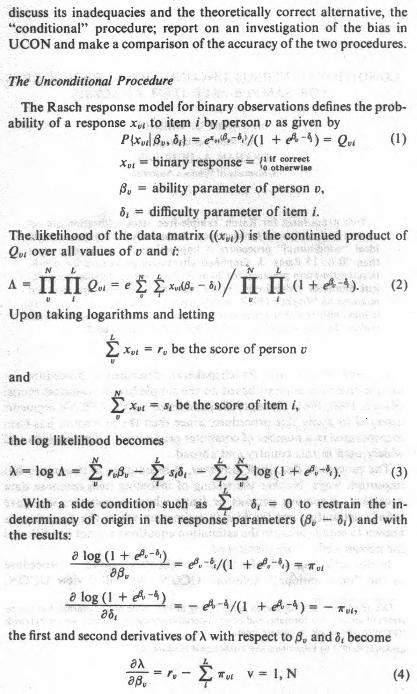
ax = Ea u , i = 1,L (6) as, a 2x

Du i ( 1 — rut) (7)

These are the equations necessary for unconditional maximum like-lihood estimation. The solutions for item difficulty estimates in equa-tions (6) and (7) depend on the presence of values for the person ability estimates. Because the data are binary, abilities can only be estimated for integer scores between 0 and L. Hence we may group persons by their score and let

b r be the ability estimate for any person with score r,

d, be the difficulty estimate of item 1,

nr be the number of persons with score r

and write the estimated probability that a person with a score r will succeed on item i as

er -A/(1 + (8)

Then L

E p„, = E nrpri

as far as estimates are concerned. A convenient algorithm for computing estimates (di ) of (S i ) is as

follows: (1) Define an initial set of (b r ) as

br ° = log (L r r)

r = 1, L — 1

(ii) Define an initial set of (di ), centered at d. = 0, as

di° = log 01 v log — = 1,L 1 Si s,

(iii) Improve each estimate d, by applying Newton-Raphson to equa-tion (6), i.e.,

L-1

+ E nrpri,

d/ L_1 r i = 1, L (9)

— E nrprii(1 — Prig)

until convergence at I c/1 1 +' — < .01

where pH' = eb, — dit /(1 + eb, — di).

and convergence to .01 is usually reached in three or four itera-tions.

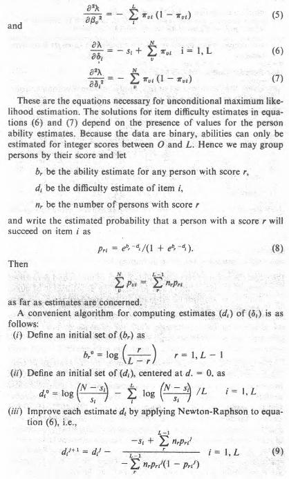
(iv) Recenter the set of (di ) at d. = 0.

(v) Using this improved set of (di ), apply Newton-Raphson to equa-tion (4) to improve each br

r — pr,'

brm+' = brm — L r = 1, L — 1 (10) - E przno - Prim)

until convergence at I b rm' — brml < .01,

where prim = eb"r — d1 /(1 + eb' — d 1 ).

(vi) Repeat steps (iii) through (v) until successive estimates of the whole set of (d,) become stable, i.e.,

E (di k+, _ diva < .0001.

which usually takes three or four cycles.

(vii) Use the negative reciprocal square root of the second derivatives defined in equation (7) and found in the denominator of equa-tion (9) as asymptotic estimates of the standard errors of each difficulty estimate, i.e.,

L -1 )- 1/2

SE(d i ) = (E nrpr, (1 - ( )

The algorithm described above is similar to the calibration tech-niques proposed by Birnbaum (1968) and Bock (1972) in that the person abilities are estimated simultaneously with the item difficulties so that the estimation procedure is not conditioned for the incidential ability parameters. However, Andersen (1970, 1971, 1972, 1973) has shown that this unconditional approach results in inconsistent esti-mates of the item parameters. The presence of the ability parameters (00 in the likelihood equation leads to biased estimates of item diffi-culties (S i ). For a procedure to produce consistent and unbiased esti-mates requires a conditional approach in which the solution equations are conditioned for the ability parameters before maximization. We

will describe the conditional solution and report on a study which supports the use of an unbiasing coefficient.

The Conditional Procedure

A conditional maximum likelihood procedure produces consistent estimates of the set of item parameters (S i) (Andersen, 1973). To develop this procedure we obtain from equation (1) the probability of the response vector (x vi) for a person whose ability parameter is 0,as

Pl(x°010v,(601 = H S r } (12)

= H ex.,4 -6,7(I + ea,-a, )

= Yud3,, — E / IT II (I + e8v -ag)

= erg, x„ ,

(I + e8,,-60.

Next we derive the probability of obtaining any score r. A person v may obtain a score r in CO different ways. Hence we

must sum all the different probabilities like (12) based on values of the response vector (x,i) which sum to r.

If we let E be the sum over all response vectors (x, i ) with E x„ 17(„1

= r and represent the elementary symmetric functions of the set of (e -6 ,) as

r _ E xr,a,

'Yr = E e , (13)

then the probability of a score r becomes

P{'l SU, (bi)} = E Pl(x„ )1 /3,, (Sr)} (14)

r _ v = eri , E e x " —A

/ 11 (1 + et - '5')

= er8, -y r (1 +

Finally, the "conditional" probability of the response vector (x vi), given the score r is obtained by dividing (12) by (14) to yield

uf)ir, (601 = Pl(xug)10,,, (1501/ P Ili (6 (15)

— E = e /7r

in Which r has replaced 0, so that (15) is not a function of Ov. If we define as the r — lth symmetric function with the element

e -a, omitted, i.e., the sum of all the ways responses to the other L — 1 items can add up to a score of r — 1, then the probability of a person with a score r getting item i correct and incorrect become

Pix„, = (16)

and

Plxvi = 01r,(601 = 7rihr•

What we have done is to condition the response model on the minimal sufficient statistic r for the incidental parameter13, The result is a conditional probability dependent only on the structural parame- ters (6,).

L For a group of N = E nr persons the conditional likelihood of

their data (s,) and (nr) is from (15) L-1

A = s '6 ' / .-yrnr (17)

Taking logarithms we have L

= log A = — E s ib, — E nr log 'Yr (18)

The derivatives of log ^y r are obtained by factoring and e - '5 J out of 7 r, i.e.,

Yr — e _fs 'Yr-1,1 + Y r,t (19)

Then a log -yr 1 a-yr _6 = = e

ao, -y r ob i

a2 log -yr = 1 3 2-yr 1 ( 87

(96,2 -yr .6 bt 2 7r2

= — (e -6' 7r-L,t/702

a 2 log -yr — 1 a 2yr ( ao,

)( a -yr a-Yr

abiao, abiab, 7, 2 \ = 7,-2,i1/7r — (e -6' 7r-1,1/7,)(e -6J 7r--1,J/7r)

If we now represent estimates of the symmetric functions y by g with

similar subscripts and define the estimated probability for a person with score r of getting item i correct as

9ri =

and the estimated probability for a person with score r of getting both items i and j correct as

grij = e- dr digr_2,,j/gr

then the three derivatives of equation (18) can be rewritten for max-imum likelihood estimation as

L-1

L* = - Sl + E nrqr, l = I, L (20)

L-1

CI1 * = E nrgri(i — gri) i = 1, L (21)

= 1, L cif * = — L nr(qrif — qr190) j = 1, L

iI (22)

A multi-parameter algorithm for obtaining the estimates and their standard errors for the polychotomous case is described by Andersen (1972). For the binary case the essential steps are:

(i) Initialize item difficulty at

[N — S i ] di° = log t log [ N

si

(ii) Use the current set of (di ) to calculate the symmetric function ratios (r -1,l/gr) and ((gr _ 2, ii/gr )) and hence (A*) and ((c ij*)) over i = 1, L and j = 1, L.

(iii) Reduce (/;*) and ((cij*)) by one item to restrain the estimation equations to a unique solution, e.g.,

= j;* — fi* i = 2, L

= — — cii * + c11* i = 2, L j = 2, L

(iv) Improve (di ) by the multi-parameter Newton-Raphson procedure

Dm -1 = Dm — [Cm] - ' P2

in which

_ _ d2 C22 • • • C2L f 2

D= , C = • • • , F=

dL C L2 • • • CLL fL - _ - _

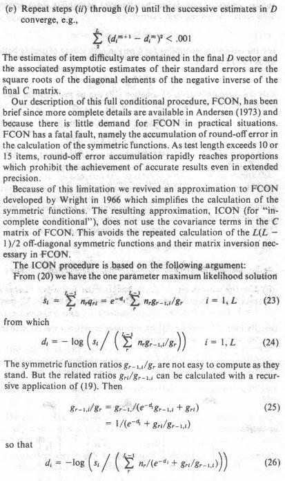
(v) Repeat steps (ii) through (iv) until the successive estimates in D converge, e.g.,

E (di m+' — dm) 2 < . 001 2

The estimates of item difficulty are contained in the final D vector and the associated asymptotic estimates of their standard errors are the square roots of the diagonal elements of the negative inverse of the final C matrix.

Our description of this full conditional procedure, FCON, has been brief since more complete details are available in Andersen (1973) and because there is little demand for FCON in practical situations. FCON has a fatal fault, namely the accumulation of round-off error in the calculation of the symmetric functions. As test length exceeds 10 or 15 items, round-off error accumulation rapidly reaches proportions which prohibit the achievement of accurate results even in extended precision.

Because of this limitation we revived an approximation to FCON developed by Wright in 1966 which simplifies the calculation of the symmetric functions. The resulting approximation, ICON (for "in-complete conditional"), does not use the covariance terms in the C matrix of FCON. This avoids the repeated calculation of the L(L — 1 )/2 off-diagonal symmetric functions and their matrix inversion nec-essary in FCON.

The ICON procedure is based on the following argument: From (20) we have the one parameter maximum likelihood solution

L-1 I = E nrqr, = e-d I nrgr-Li/gr i = 1, L (23)

from which

d, = — log nT o -or-1,14r)) = 1, L (24)

The symmetric function ratios gr _ L i/gr are not easy to compute as they stand. But the related ratios g /g arl, 0,r -1,i can be calculated with a recur- sive application of (19). Then

gr = + gri) (25)

= 1/(c`4 + gagr--1,t)

so that L-1

d = —log (s, E nr/(e-d , + gri/g,_,,,))) (26)

The steps are:

(i) Initialize (d1 ) at cl,°. (ii) Use the current set of (di ) in the right hand side of (26) and obtain

a revised estimate for each di on the left side. (iii) Recenter the (d1 ). (iv) Use the revised set (di ) to recalculate the and repeat

steps (ii) and (iv) until convergence is obtained. (v) At convergence, estimate the standard error from the second

derivative of the likelihood equation as in (21).

ICON takes less computer space and less time for each iteration than FCON, but the total number of iterations required is slightly greater because we have ignored the covariances in C. In trials under a variety of conditions we have found no difference between the esti-mates obtained by FCON and ICON. For example, in three replica-tions of the simulated administration of a 40-item test (in which we generated uniformly distributed item parameters with center at (5 = 0 and range ±2 and then disturbed them by random fluctuations with standard deviation 0.1) to 100 subjects (with mean ability 13 = 2.0, standard deviation .5 and skewed by truncating Q < 3) the maximum discrepancy between an FCON estimate and an ICON estimate was .03 logits.

As a result we dropped FCON from further consideration as an efficient and reasonable estimation algorithm and concentrated on ICON. Although convergence was always obtained from ICON we were limited in our study of its performance by the fact that fatal round-off errors accumulated when there were more than 20 or 30 items in the test, especially in the presence of extreme item parameters. This produced estimates which were biased when compared with the parameters used to generate the simulated data. Thus even ICON was not practical enough.

We had hoped that a useful algorithm could be derived from our study of the theoretically ideal conditional procedure. It is conceivable that fuller use of extended precision and a different organization of the iteration sequence might lead to the practical conditional procedure we were seeking. But we were unable to achieve this. So we turned our attention to an investigation of the extent and direction of the bias in the unconditional procedure UCON.

The Bias in the Unconditional Procedure

Our approach to evaluating the bias in the unconditional estimation procedure commences with the likelihood equations (6) and (20)

which connect parameters and data for FCON and UCON. From.(6) we have

L-1

St = E nrebr- d ,* /( 1 + .") (27)

in which di * is the biased UCON estimate of d t . From (20) we have

St = nre- d gr - 1,1/gr •

But, since g,. = + gri, we can write

(gr- agr) = (gr- i.t/grt Kgr/grt)

(gr-1,1/grt)/(1 + e -d4gr-1,1/grt))•

Were we to extend our analysis of FCON to derive functions of (d,)

which yield optimal ability estimates b r we would find br = log(gr _,/gr ) to be a maximum likelihood solution. If we define the ability estimate that goes with a score of r when item i is removed from the test as brt , then we may let

vv r-1,t/gri

and the FCON estimation equation becomes

St = 1 nrebri-d,/(1 + eb- - d , ) (28)

Since (27) and (28) estimate similar parameters for identical data,

bri = br — d i *.

Thus the bias in the UCON estimate of item i difficulty at score r, when compared with the unbiased d, from FCON is

br — bri = art. (29)

Our aim is to find a way to correct d,* for this bias. The simplest scheme would be to find a correction factor k = di /di *. If we define ert = an/di as the relative bias in the difficulty estimate of item i at score r

then

k = di/d,* = di/(d, + art ) .= 1/(1 + crt). (30)

We explored the possibilities for k by studying how values of a rt and cri vary over r and d, in a wide variety of typical test structures. For each test we

(1) Specified test length L and standard deviation Z for a normal distribution of item difficulties.

(ii) Generated the consequent set of item difficulties (di ). (iii) Calculated from (di ) the log symmetric function ratios

br = log (gr_i/gr)

bri = log (gr-i,i/gri),

(iv) and hence the biases

ari '= br - bri

cri = ari/di except 1c/1 1 < .5.

(v) Calculated the average relative bias L L

CAA = E E ri -

c /(L 1)(L) except 1d11 < . 5

r i

as a basis for estimating k, The results were systematic. They are summarized in Table 1 for a

series of normally shaped tests of lengths L = 20, 30, 40, 50 and 80 and item difficulty standard deviations of Z = 1.0, 1.5, 2.0, 2.5.

The values of c in Table 1 are well approximated by 1/(L - I) regardless of Z.

If c.. 1/(L - 1),

then k 1/(1 + 1/(L - 1)) = (L - 1)/L. (31)

This is the correction factor used in most versions of UCON and coincides with the correction deducible in the simple case where L = 2 and the UCON estimates can be shown to be exactly twice the FCON ones. Thus the corrected UCON procedure is indistinguishable from ICON or FCON in the practice of item calibration.

TABLE 1 Relative Bias in the Unconditional Procedure

(Averaged over Items and Scores)

Test Test Dispersion in Item Std. Dev.s 1

Length 1.0 1.5 2.0 2.5 L - 1

20 .0525 .0525 .0560 .0522 .0526 30 .0345 .0320 .0349 .0349 .0345 40 .0238 .0258 .0261 .0252 .0256 50 .0203 .0192 .0195 .0199 .0204 80 .0126 .0124 .0121 .0127 .0126

L - 1 L

Mean Relative Bias c.. = E E c,,/(L- I)(L) A

where c,, = aad,

= b, - b,, (71,* - d,, the bias.

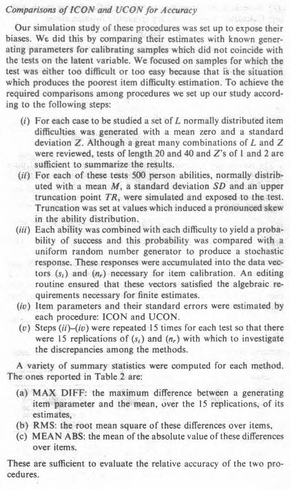
Comparisons of ICON and UCON for Accuracy

Our simulation study of these procedures was set up to expose their biases. We did this by comparing their estimates with known gener-ating parameters for calibrating samples which did not coincide with the tests on the latent variable. We focused on samples for which the test was either too difficult or too easy because that is the situation which produces the poorest item difficulty estimation. To achieve the required comparisons among procedures we set up our study accord-ing to the following steps:

(i) For each case to be studied a set of L normally distributed item difficulties was generated with a mean zero and a standard deviation Z. Although a great many combinations of L and Z were reviewed, tests of length 20 and 40 and Z's of 1 and 2 are sufficient to summarize the results.

(ii) For each of these tests 500 person abilities, normally distrib-uted with a mean M, a standard deviation SD and an upper truncation point TR, were simulated and exposed to the test. Truncation was set at values which induced a pronounced skew in the ability distribution.

(iii) Each ability was combined with each difficulty to yield a proba-bility of success and this probability was compared with a uniform random number generator to produce a stochastic response. These responses were accumulated into the data vec-tors (s 1 ) and (nr ) necessary for item calibration. An editing routine ensured that these vectors satisfied the algebraic re-quirements necessary for finite estimates.

(iv) Item parameters and their standard errors were estimated by each procedure: ICON and UCON.

(v) Steps (ii) — (iv) were repeated 15 times for each test so that there were 15 replications of (si ) and (nr ) with which to investigate the discrepancies among the methods.

A variety of summary statistics were computed for each method. The ones reported in Table 2 are:

(a) MAX DIFF: the maximum difference between a generating item parameter and the mean, over the 15 replications, of its estimates,

(b) RMS: the root mean square of these differences over items, (c) MEAN ABS: the mean of the absolute value of these differences

over items.

These are sufficient to evaluate the relative accuracy of the two pro-cedures.

TABLE 2 Comparison of ICON and UCON for Normal Tests and Truncated Samples

(Based on 15 Replications of 500 Persons Each)

DATA PROCEDURES Test Sample ICON UCON

MAX MEAN MAX MEAN Case L Z M SD TR DIFF RMS ABS DIFF RMS ABS

1 20 1 0 0.5 2.0 .05 .03 .08 - .05 .02 .08 2 20 1 0 1.0 2.0 - .07 .03 .08 - .06 .03 .08 3 20 1 1 1.0 2.5 .08 .03 .09 - .06 .03 .09 4 20 1 1 1.5 2.0 -.05 .03 .09 -.07 .03 .09 5 20 I 1 1.5 2.5 .24 .06 .10 -.07 .03 .10

6 40 1 0 0.5 2.0 -.08 .03 .08 - .08 .03 .08 7 40 I 0 1.0 2.0 .13 .03 .08 -.07 .03 .08 8 40 1 1 1.0 2.5 .11 .03 .08 -.II .03 .09 9 40 1 1 1.5 2.0 .15 .04 .09 .06 .03 .09

10 40 1 1 1.5 2.5 .27 .06 .09 .07 .03 .09

11 40 2 0 2.0 4.5 .31 .07 .10 -.12 .05 .10 12 40 2 2 2.0 4.5 .42 .11 .13 -.30 .06 .12

Where MAX DIFF: the maximum difference between a generating item parameter and the mean, over 15

replications, of its estimates,

RMS: the root mean square of these differences over items,

MEAN ABS: the mean of the absolute value of these differences over items.

In terms of the RMS and MEAN ABS there is little to choose between the procedures, no matter what the test and sample character-istics, so our discussion is confined to the MAX DIFF's. When the items are most appropriate for the calibrating sample (cases 1, 2, 6 and 7) there are no discernible differences between the two procedures. As the mean of the sample shifts away from zero, however (M = 1 or 2), or the severity of truncation and hence skew increases, then the MAX DIFF's tend to increase for both algorithms and particularly for ICON. This latter phenomenon was found to be due to the increasing discrepancy between item and sample characteristics which produced extreme item parameters that are never reasonably estimated by ICON because of accumulated round-off error in the calculation of the symmetric functions.

REFERENCES

Andersen, E. B. Asymptotic properties of conditional maximum likeli-hood estimators. Journal of the Royal Statistical Society. 1970, 32, 283-301.

Andersen, E. B. The asymptotic distribution of conditional likelihood ratio tests. Journal of the American Statistical Association, 1971, 66 (335), 630-33.

Andersen, E. B. The numerical solution of a set of conditional estima-tion equations. The Journal of the Royal Statistical Society; Series B, 1972, 34 (1), 42-54.

Andersen, E. B. Conditional Inference and Models for Measuring. Cophenhagen, Denmark: Mentalhygiejnisk Forlag, 1973.

Birnbaum, A. Estimation of an ability. In F. Lord and M. Novick (Eds.), Statistical Theories of Mental Test Scores. Reading, Mass.: Addison-Wesley, 1968.

Bock, R. D. Estimating item parameters and latent ability when responses are scored in two or more nominal categories. Psycho-metrika, 1972, 37, 29-51.

Rasch, G. Probabilistic Models for Some Intelligence and Attainment Tests. Copenhagen, Denmark: Denmarks Paedagogiske Institut, 1960.

Rasch, G. On general laws and the meaning of measurement in psy-chology. Proceedings of the Fourth Berkeley Symposium on Mathe-matical Statistics, 1961, 4, 321-33.

Rasch, G. An individualistic approach to item analysis. In P. F. Lazarsfeld and N. W. Henry (Eds.), Readings in Mathematical Social Sciences. Chicago: Science Research Associates, 1966. (a)

Rasch, G. An item analysis which takes individual differences into account. British Journal of Mathematical and Statistical Psychol-ogy, 1966, 19, 49-57. (b)

Wright, B. D. and Panchapakesan, N. A procedure for sample-free item analysis, EDUCATIONAL AND PSYCHOLOGICAL MEASUREMENT, 1969, 29, 23-48.