Embed Size (px)
Citation preview
Nonsmooth dynamical systemson stability of hybrid trajectories andbifurcations of discontinuous systems
Benjamin Biemond

The research leading to the results presented in this thesis has received funding fromthe Netherlands Organisation for Scientific Research (NWO), the European UnionSixth Framework Program under grant no. FP6-IST-511368 HYCON Network ofExcellence and the European Union Seventh Framework Programme(FP7/2007-2013) under grant agreement no. 257462 HYCON2 Network of Excellence.
A catalogue record is available from the Eindhoven University of Technology Library.ISBN: 978-90-386-3337-4
c©2012 by J.J.B. Biemond. All rights reserved.

Nonsmooth dynamical systemson stability of hybrid trajectories andbifurcations of discontinuous systems
PROEFSCHRIFT
ter verkrijging van de graad van doctor aan deTechnische Universiteit Eindhoven, op gezag van de
rector magnificus, prof.dr.ir. C.J. van Duijn, voor eencommissie aangewezen door het College voor
Promoties in het openbaar te verdedigenop dinsdag 12 maart 2013 om 16.00 uur
door
Jan Jacobus Benjamin Biemond
geboren te Rotterdam

Dit proefschrift is goedgekeurd door de promotor:
prof.dr. H. Nijmeijer
Copromotor:dr.ir. N. van de Wouw

Contents
1 Introduction 1
1.1 Nonsmooth systems . . . . . . . . . . . . . . . . . . . . . . . . . 1
1.2 Motivation and objectives . . . . . . . . . . . . . . . . . . . . . . 5
1.2.1 Bifurcation analysis . . . . . . . . . . . . . . . . . . . . . 5
1.2.2 Tracking control for hybrid systems . . . . . . . . . . . . 7
1.3 Main contributions . . . . . . . . . . . . . . . . . . . . . . . . . . 8
1.4 Outline of this thesis . . . . . . . . . . . . . . . . . . . . . . . . . 10
I Bifurcation analysis of nonsmooth systems 13
2 Nonsmooth bifurcations of equilibria in planar continuous sys-tems 15
2.1 Introduction . . . . . . . . . . . . . . . . . . . . . . . . . . . . . . 15
2.2 Preliminaries . . . . . . . . . . . . . . . . . . . . . . . . . . . . . 17
2.3 Stability of an equilibrium at the bifurcation point . . . . . . . . 20
2.3.1 Systems with visible eigenvectors . . . . . . . . . . . . . . 20
2.3.2 Systems without visible eigenvectors . . . . . . . . . . . . 22
2.3.3 Stability result . . . . . . . . . . . . . . . . . . . . . . . . 23
2.4 Bifurcation analysis of a conewise affine system . . . . . . . . . . 24
2.4.1 Trajectories visiting a cone Si . . . . . . . . . . . . . . . . 26
2.4.2 Construction of the return map . . . . . . . . . . . . . . . 26
2.4.3 Procedure to obtain all closed orbits . . . . . . . . . . . . 27
2.5 Approximation effects . . . . . . . . . . . . . . . . . . . . . . . . 29
2.6 Illustrative examples . . . . . . . . . . . . . . . . . . . . . . . . . 32
2.6.1 Example for a conewise affine system . . . . . . . . . . . . 32
2.6.2 Example for a piecewise smooth system . . . . . . . . . . 34
2.7 Conclusions . . . . . . . . . . . . . . . . . . . . . . . . . . . . . . 39

ii Contents
3 Bifurcations of equilibrium sets in mechanical systems 413.1 Introduction . . . . . . . . . . . . . . . . . . . . . . . . . . . . . . 413.2 Modelling and main result . . . . . . . . . . . . . . . . . . . . . . 433.3 Structural stability of the system near the equilibrium set . . . . 47
3.3.1 Structural stability of planar systems . . . . . . . . . . . . 483.4 Bifurcations . . . . . . . . . . . . . . . . . . . . . . . . . . . . . . 50
3.4.1 Real or complex eigenvalues . . . . . . . . . . . . . . . . . 513.4.2 Zero eigenvalue . . . . . . . . . . . . . . . . . . . . . . . . 523.4.3 Closed orbits . . . . . . . . . . . . . . . . . . . . . . . . . 53
3.5 Illustrative example . . . . . . . . . . . . . . . . . . . . . . . . . 543.6 Conclusion . . . . . . . . . . . . . . . . . . . . . . . . . . . . . . 563.7 Comparison with existing results on bifurcations and structural
stability of discontinuous systems . . . . . . . . . . . . . . . . . . 58
4 Dynamical collapse of trajectories 614.1 Introduction . . . . . . . . . . . . . . . . . . . . . . . . . . . . . . 614.2 Model of a pendulum with dry friction . . . . . . . . . . . . . . . 634.3 Local behaviour . . . . . . . . . . . . . . . . . . . . . . . . . . . . 644.4 Homoclinic or heteroclinic orbits . . . . . . . . . . . . . . . . . . 654.5 Return map of trajectories around a homoclinic orbit . . . . . . . 674.6 Chaotic saddle . . . . . . . . . . . . . . . . . . . . . . . . . . . . 684.7 Conclusion . . . . . . . . . . . . . . . . . . . . . . . . . . . . . . 70
5 Horseshoes in discrete-time systems described by non-invertiblemaps 715.1 Introduction . . . . . . . . . . . . . . . . . . . . . . . . . . . . . . 715.2 Discrete-time dynamical system . . . . . . . . . . . . . . . . . . . 74
5.2.1 Motivating numerical example . . . . . . . . . . . . . . . 755.2.2 Definition of the discrete-time system . . . . . . . . . . . 775.2.3 Geometry of the limit set . . . . . . . . . . . . . . . . . . 80
5.3 Symbolic dynamics . . . . . . . . . . . . . . . . . . . . . . . . . . 825.4 Topological conjugacy between symbolic dynamics and discrete-
time system . . . . . . . . . . . . . . . . . . . . . . . . . . . . . . 845.5 Conclusion . . . . . . . . . . . . . . . . . . . . . . . . . . . . . . 86
II Tracking control for hybrid systems 87
6 Tracking control for hybrid systems with state-triggered jumps 896.1 Introduction . . . . . . . . . . . . . . . . . . . . . . . . . . . . . . 896.2 Modelling of hybrid control systems . . . . . . . . . . . . . . . . 936.3 Formulation of the tracking control problem . . . . . . . . . . . . 96
6.3.1 Definition of the tracking error measure . . . . . . . . . . 966.3.2 Tracking problem formulation . . . . . . . . . . . . . . . . 98
Contents iii
6.4 Sufficient conditions for stability withrespect to d . . . . . . . . . . . . . . . . . . . . . . . . . . . . . . 1006.4.1 Closed-loop solutions . . . . . . . . . . . . . . . . . . . . . 1006.4.2 Lyapunov-type stability conditions . . . . . . . . . . . . . 101
6.5 Tracking controller design for exemplarysystems . . . . . . . . . . . . . . . . . . . . . . . . . . . . . . . . 1046.5.1 Global tracking for a scalar hybrid system . . . . . . . . . 1046.5.2 Tracking control for the bouncing ball . . . . . . . . . . . 107
6.6 Conclusion . . . . . . . . . . . . . . . . . . . . . . . . . . . . . . 111
7 Conclusions and recommendations 1157.1 Conclusions . . . . . . . . . . . . . . . . . . . . . . . . . . . . . . 1157.2 Recommendations . . . . . . . . . . . . . . . . . . . . . . . . . . 117
A Proofs and technical results 121A.1 Appendices of Chapter 2 . . . . . . . . . . . . . . . . . . . . . . . 122
A.1.1 Computation of maps gi, i = 1, . . . ,m. . . . . . . . . . . . 122A.1.2 Proofs . . . . . . . . . . . . . . . . . . . . . . . . . . . . . 123
A.2 Appendices of Chapter 3 . . . . . . . . . . . . . . . . . . . . . . . 141A.2.1 Existence of an equilibrium set . . . . . . . . . . . . . . . 141A.2.2 Proof of Theorem 3.1 . . . . . . . . . . . . . . . . . . . . 145A.2.3 Proof of Theorem 3.2 . . . . . . . . . . . . . . . . . . . . 148A.2.4 Proof of Lemma 3.3 . . . . . . . . . . . . . . . . . . . . . 154
A.3 Proofs of theorems and lemmas of Chapter 5 . . . . . . . . . . . 156A.4 Local phase portrait near an equilibrium set of a periodically
forced mechanical system with dry friction . . . . . . . . . . . . . 166A.4.1 Unperturbed system dynamics . . . . . . . . . . . . . . . 166A.4.2 Effect of a time-dependent perturbation . . . . . . . . . . 168
A.5 Appendices of Chapter 6 . . . . . . . . . . . . . . . . . . . . . . . 182A.5.1 Proof of Theorem 6.1 . . . . . . . . . . . . . . . . . . . . 182A.5.2 Proof of Theorem 6.2 . . . . . . . . . . . . . . . . . . . . 183A.5.3 Proof of Theorem 6.3 . . . . . . . . . . . . . . . . . . . . 184A.5.4 Proof of Theorem 6.4 . . . . . . . . . . . . . . . . . . . . 184A.5.5 Proof of Theorem 6.5 . . . . . . . . . . . . . . . . . . . . 185A.5.6 Proof of Theorem 6.6 . . . . . . . . . . . . . . . . . . . . 186
Bibliography 189
Abstract 201
Samenvatting 203
Dankwoord 205
List of publications 207
Curriculum vitae 209

Chapter 1
Introduction
1.1 Nonsmooth systems
Nonsmooth systems are used to model various dynamical behaviours in physics,engineering, biology, and economy. In these models, nonsmooth elements areadded such that complex dynamical characteristics can be captured. In thismanner, nonsmooth systems are obtained that can provide a dynamical modelat a level of abstraction that is appropriate for design, analysis or control pur-poses. In this thesis, the qualitative dynamical behaviour and the stability ofnonsmooth systems are analysed to support the application of such systems.
To illustrate one of the dynamical characteristics that are effectively modelledwith nonsmooth elements, observe that a printed copy of this thesis does notshow any motion shortly after it has been placed on a desk, even though the deskits surface is probably not perfectly horizontal. Hence, the thesis arrives at anequilibrium position in a finite time. If Newton’s second law is used to describethis dynamics, then a discontinuous force model for the friction between the deskand the thesis, e.g. Coulomb’s friction law, can accurately model the observedbehaviour, without the infinitely long transient behaviour that is expected insmooth differential equations, and without the need to model the detailed profileof the surface of the desk.
Next to the possibility to attain equilibrium positions in finite time, thisexample illustrates another reason to employ nonsmooth dynamical models. Ifthe desk with the thesis is slightly tilted, no motion is expected, and the thesiswill stick to its original position. Consequently, the equilibrium position is com-pletely robust with respect to certain perturbations, including small tilting ofthe desk. Equilibrium points of smooth differential equations will not showsuch robustness properties, whereas a discontinuous dynamical model that uses

2 Chapter 1. Introduction
Coulomb’s friction law does effectively represent this behaviour.In addition to finite-time convergence and different robustness properties,
various other properties of dynamical systems have motivated the use of non-smooth models. For example, nonsmooth systems provide an effective methodto model dynamical behaviour that combines slow and fast motions. If thetimescales of the slow and fast motions are far apart, then smooth differen-tial equations will have steep gradients. This makes their numerical simulationcumbersome, and complicates the application of conventional results on stabil-ity, control and robustness. A way to proceed is to model the fast phenomena tooccur instantaneously. In mechanical systems with unilateral constraints, thisapproach leads to nonsmooth dynamical models with idealised contact and im-pact laws. Such models are called hybrid systems, and contain both continuous-time evolution and discrete events, i.e. instantaneous jumps in the system states,that represent the fast phenomena. Hybrid systems form an important subset ofthe class of nonsmooth systems. Hybrid models can also be employed to modelsystems that feature both continuous evolution in time and discrete events, asis e.g. apparent in switching control systems.
Nonsmooth systems have been used to model dynamical behaviour in variousdisciplines. In mechanical engineering, the interaction between rigid bodies canbe modelled using nonsmooth force laws for contact, impact and friction, leadingto nonsmooth dynamical systems, cf. [66, 103, 104, 125, 159]. In control engin-eering, sliding mode controllers [144, 154], controller saturation [150], switchingpiecewise affine controllers [50,109], and networked control systems [78] are usu-ally modelled with nonsmooth dynamical systems. In various control systems,including sliding mode controllers and control systems with hysteresis elements,nonsmooth elements are intentionally introduced in the closed-loop system to ex-ploit properties that are specific to nonsmooth systems, such as finite-time tran-sients or increased robustness, cf. [136, 144]. In electrical engineering, switches(relays) and diodes can induce nonsmooth dynamical behaviour, cf. e.g. [3,14,65].Nonsmooth dynamical models are also used in other disciplines, such as phys-ics [89], biology [113] and economics [124].
This thesis is focussed on nonsmooth systems that display continuous-timeevolution, and dynamical systems described by difference equations (i.e. itera-tions of maps) are only used as an analysis tool for nonsmooth systems withcontinuous-time evolution. The class of continuous-time systems with non-smooth behaviour, as studied in this thesis, can be classified in the followingthree cases with increasing degree of nonsmoothness, cf. [15, 102,103,143]:
• Non-differentiable systems – Systems described by a continuous differen-tial equation that is piecewise smooth, such that it is non-differentiableonly at some (n−1)-dimensional surfaces in an n-dimensional state space.An example is given by a mechanical system with a one-sided spring, cf.Fig. 1.1. Despite the non-differentiability of the right-hand side, these dif-ferential equations still satisfy a local Lipschitz’s condition, see e.g. [91],

1.1 Nonsmooth systems 3
Non-differentiablesystems
Mx+ cx+ g =0, x ≥ 0−kx, x < 0
Discontinuoussystems
Mx+ kx+ cx ∈ −µMg, x > 0[−µMg, µMg] , x = 0
µMg, x < 0
Hybrid systemsMx+cx = −Mg, x > 0impact+unilat-eral contact law,
x = 0
Fig. 1.1. Examples of the three types of nonsmooth systems.
such that the standard definition of solutions for differential equations canbe applied. Consequently, for a given initial condition, a unique solutioncurve is found that is differentiable with respect to time. The lack of dif-ferentiability of the vector field renders existing results on stability androbustness for smooth systems inapplicable when they rely on local linear-isation. For example, the indirect method of Lyapunov to study stability,cf. [91], and the Hartman-Grobman theorem to study robustness, cf. [74],can no longer be employed.
• Discontinuous systems – Systems described by an n-dimensional differen-tial equation that is piecewise smooth and contains discontinuities at some(n − 1)-dimensional surfaces in the state space. For example, Coulomb’s
4 Chapter 1. Introduction
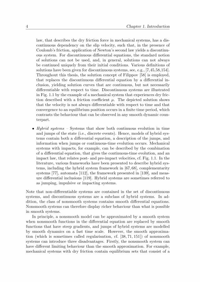
law, that describes the dry friction force in mechanical systems, has a dis-continuous dependency on the slip velocity, such that, in the presence ofCoulomb’s friction, application of Newton’s second law yields a discontinu-ous system. For discontinuous differential equations, the standard notionof solutions can not be used, and, in general, solutions can not alwaysbe continued uniquely from their initial conditions. Various definitions ofsolutions have been given for discontinuous systems, see, e.g., [7,45,58,154].Throughout this thesis, the solution concept of Filippov [58] is employed,that replaces the discontinuous differential equation by a differential in-clusion, yielding solution curves that are continuous, but not necessarilydifferentiable with respect to time. Discontinuous systems are illustratedin Fig. 1.1 by the example of a mechanical system that experiences dry fric-tion described with a friction coefficient µ. The depicted solution showsthat the velocity is not always differentiable with respect to time and thatconvergence to an equilibrium position occurs in a finite time period, whichcontrasts the behaviour that can be observed in any smooth dynamic coun-terpart.
• Hybrid systems – Systems that show both continuous evolution in timeand jumps of the state (i.e., discrete events). Hence, models of hybrid sys-tems contain both a differential equation, a description of the jumps, andinformation when jumps or continuous-time evolution occurs. Mechanicalsystems with impacts, for example, can be described by the combinationof a differential equation, that gives the continuous-time evolution, and animpact law, that relates post- and pre-impact velocities, cf. Fig. 1.1. In theliterature, various frameworks have been presented to describe hybrid sys-tems, including the hybrid system framework in [67, 68], complementaritysystems [77], automata [112], the framework presented in [139], and meas-ure differential inclusions [119]. Hybrid systems are sometimes referred toas jumping, impulsive or impacting systems.
Note that non-differentiable systems are contained in the set of discontinuoussystems, and discontinuous systems are a subclass of hybrid systems. In ad-dition, the class of nonsmooth systems contains smooth differential equations.Nonsmooth systems can therefore display richer behaviour than what is possiblein smooth systems.
In principle, a nonsmooth model can be approximated by a smooth systemwhen nonsmooth functions in the differential equation are replaced by smoothfunctions that have steep gradients, and jumps of hybrid systems are modelledby smooth dynamics on a fast time scale. However, the smooth approxima-tion (which is sometimes called regularisation, cf. [38, 71, 151]) of nonsmoothsystems can introduce three disadvantages. Firstly, the nonsmooth system canhave different limiting behaviour than the smooth approximation. For example,mechanical systems with dry friction contain equilibrium sets that consist of a

1.2 Motivation and objectives 5
continuum of non-isolated equilibrium positions, whereas a smooth approxim-ation will only show isolated equilibrium points. Secondly, the effect of smallperturbations of the vector field is different for nonsmooth systems and their reg-ularised version. Finally, smooth differential equations that describe nonsmoothphenomena, generically, have steep gradients, which make such smooth modelsless suited for simulation purposes.
1.2 Motivation and objectives
In this thesis, two different problems are considered in nonsmooth dynamicalsystems. Consequently, the thesis consists of two parts. In Part I, that con-tains Chapters 2-5, the effect of small parameter variations on the qualitativebehaviour of nonsmooth systems is studied and, in particular, bifurcations inseveral classes of nonsmooth systems are investigated. In Part II, that consistsof Chapter 6, the tracking control problem for hybrid systems is considered. Inthe present section, the motivation for both research topics is given. This in-troductory chapter is written in a concise fashion to highlight the motivationand contributions of the thesis. Detailed literature surveys are presented in theindividual chapters.
1.2.1 Bifurcation analysis
The qualitative behaviour of a dynamical system is mainly determined by itslimit sets, the stability of the limit sets, and the trajectories converging to, ordiverging from these sets. Limit sets consist of the points in the state space towhich trajectories tend when time evolves to infinity, or from which trajectorieshave diverged in the past. Examples of limit sets are equilibria and periodicorbits. In general, small changes of a dynamical system will only change thedynamics quantitatively, and such changes will not induce qualitative changesof the limit sets. Loosely speaking, changes in the qualitative behaviour of adynamical system, such as the loss of stability of an equilibrium point or thecreation of a new limit set, are called bifurcations when they are caused by avariation in a system parameter. A formal definition of bifurcations will be givenin Chapter 2. We note that bifurcations induce structural changes in the phaseportrait of a dynamical system.
A dynamical system is called structurally stable when small perturbationsof the system cannot induce qualitative changes in its behaviour. Hence, anarbitrary small variation of the system parameters may induce qualitatively dif-ferent dynamics only when a system is not structurally stable. Consequently,structural stability excludes the occurrence of bifurcations, and vice versa.
The study of structural stability and bifurcations in dynamical systems is mo-tivated in two ways. Firstly, structural stability and bifurcation results give im-portant insight in the robustness to parameter variations in the analysis, design

6 Chapter 1. Introduction
and modelling of dynamical systems. When the amplitude of an external disturb-ance is considered as a system parameter, knowledge on the possible bifurcationscan be used to assess the robustness for disturbances. Secondly, the study ofbifurcations allows to explore the types of behaviour that can be displayed bya given dynamical system, thereby giving insight in the overall dynamics. Suchinsight can, for example, be instrumental in supporting the design of robustsystems.
The theory of bifurcations and structural stability in smooth dynamical sys-tems is well developed, cf. [72, 95, 127, 132, 142, 145], and hinges on dimensionreduction by methods such as the center manifold theorem, cf. [43] and normalhyberbolicity, cf. [57, 142], and the analysis of low-dimensional systems usingnormal forms, which, in the simplest cases, can be obtained using linearisation,cf. [74].
In nonsmooth dynamical systems, both dimension reduction techniques andbifurcations in low-dimensional systems are not well understood and are still sub-ject to ongoing research. In Part I of this thesis, bifurcations of low-dimensionalsystems are discussed. The development of dimension reduction techniques fallsoutside the scope of this thesis.
A large portion of the current literature on bifurcation theory for nonsmoothdynamical systems deals with non-differentiable or discontinuous systems of lowdimensions (in particular, systems with a two or three dimensional state space),see e.g. [15,103,114]. Moreover, most results are focussed on bifurcations of thelocal dynamical behaviour near limit cycles and isolated equilibrium points. Itis common to assume that the nonsmooth behaviour is localised to one surfacein the state space, and away from this surface, trajectories are described by alocally smooth differential equation.
In the neighbourhood of limit cycles, bifurcation scenarios have been iden-tified where, due to parameter variation, a limit cycle becomes tangential to asurface where the vector field is nonsmooth, or when a limit cycle arrives at apoint where this surface is not-differentiable, e.g. makes a sharp corner. Bifurc-ations induced by such interactions are called grazing and boundary crossingbifurcations, respectively, cf. [8, 15, 47, 58, 123, 155]. Normally, such bifurcationsare investigated using a Poincare return map, see e.g. [138], that reduces theproblem to the analysis of the iterates of a non-differentiable or discontinuousdifference equation.
Various bifurcations have been investigated that can occur in the neighbour-hood of equilibrium points for nonsmooth systems, see e.g. [14,56,58,103]. Classi-fication of these bifurcations has yielded lists of bifurcations in non-differentiableand discontinuous systems, as can be found in [14,71,96,143,151]. In these stud-ies, systems are considered where the discontinuity of the vector field is restrictedto an n-1-dimensional surface in the n-dimensional state space. The vector fieldson both sides of this surface are chosen to be two arbitrary vector fields withno relation between them, (in contrast to, e.g., models of mechanical systems

1.2 Motivation and objectives 7
with dry friction, where the difference between the vector field on both sides ofthe discontinuity is constant). Certain behaviour that does occur in physicalsystems, (e.g. the existence of non-isolated equilibrium positions in mechanicalsystems with friction) will be considered highly non-generic in this approach. Onthe other hand, some bifurcations that occur generically according to the listspresented in [14, 71, 96, 143, 151] have not yet been observed in discontinuoussystem models of physical systems.
The bifurcation analysis presented in Chapter 2 can be considered as anextension of this line of research towards the case where, in the neighbour-hood of an equilibrium point, the nonsmoothness is not completely located on asingle smooth 1-dimensional surface (i.e. a smooth curve) in the 2-dimensionalstate space, but either a single non-differentiable curve, or multiple intersectingcurves are required to describe the set where the vector field is non-differentiable.Hence, the approach presented in Chapter 2 can be used to study the case wherethree or more distinct domains are present in which the trajectories are describedwith different smooth differential equations. The results in Chapter 2 also illus-trate that a complete classification of all possible bifurcations will be very hard toachieve, as this classification should contain very diverse bifurcation scenarios,even when restricted to the simple case of non-differentiable two-dimensionalsystems.
In [86, 163] and Chapters 3-5, an alternative approach is pursued, namely,structural stability and bifurcations of specific nonsmooth systems are investig-ated, that model mechanical systems with dry friction. This restricts the class ofvector fields under study, such that dynamical behaviour appears that is rathernon-generic in the full class of discontinuous systems, but which does corres-pond to behaviour that is highly relevant in mechanical systems. In particular,equilibrium points are, in general, not isolated for mechanical systems with dryfriction, but appear in connected sets of non-isolated equilibrium points, which,in this thesis, are called equilibrium sets. In Chapter 3, structural stability andbifurcations are investigated of the local vector field near such equilibrium sets.In Chapter 4, the effect on the dynamics of this system is discussed of periodicperturbations, and a new type of limit set is discovered that can be induced bythe perturbation of such discontinuous differential equations. The new limit sethas some interesting analogies with chaotic saddles found in smooth systems,cf. [98, 145]. In Chapter 4, the properties of the limit set are analysed by con-struction of a Poincare return map. Motivated by this argument, in Chapter 5,we analyse the dynamics of such maps in more detail.
1.2.2 Tracking control for hybrid systems
In Part II of this thesis, the tracking control problem for hybrid systems isstudied. In tracking control problems, a control law should be designed suchthat a given physical system, that is called the plant and that is modelled as a

8 Chapter 1. Introduction
dynamical system with inputs, performs a task by following a pre-described ref-erence trajectory. Since initial conditions of the plant will not be exactly known,the controller should induce asymptotic stability of the reference trajectory. Inwords, the stability of a trajectory implies that, if another trajectory is initiallyclose, it remains close in the future. Asymptotic stability implies, in addition tostability, that both trajectories tend towards each other over time. In this part,a notion of stability of trajectories is formulated that can be applied to hybridsystems with state-triggered jumps, and show that this notion is instrumentalin the design of a control law solving the tracking problem.
In smooth systems, the stability of a trajectory is conventionally analysed byevaluation of the difference between the given trajectory and trajectories withnearby initial conditions, cf. [130, 157]. Usually, the evolution of this differenceover time is called the error system. The asymptotic stability of the giventrajectory is equivalent to the asymptotic stability of the origin for the errorsystem, which is commonly defined in the sense of Lyapunov, cf. [91].
In non-differentiable or discontinuous dynamical systems, this stability no-tion can directly be employed. However, for hybrid systems, this approach isnot always satisfactory. Namely, the jump times of two trajectories of a hybridsystem do not necessarily coincide, i.e. they may display a small timing mis-match. During this time interval, the Euclidean distance between the states ofboth trajectories is expected to be large. Hence, the conventional Euclidean er-ror between both trajectories cannot be made arbitrarily small by selecting theinitial conditions sufficiently close, contradicting asymptotic stability in termsof the Euclidean distance, as observed e.g. in [75,104,116]. A small timing mis-match of the jumps (converging to zero over time), however, does not alwayscontradict desired behaviour. For this reason, asymptotic stability, evaluated interms of the Euclidian distance between the states of two hybrid systems, canbe infeasible, even though intuitively desirable behaviour can still be achieved.
In Part II of this thesis, we propose a novel notion for the stability of tra-jectories for hybrid systems, that does not require that jump times coincide, butstill corresponds to an intuitive notion of stability for jumping solutions. Usingthis notion of stability, in Chapter 6, a tracking control problem is formulatedthat is feasible for a larger class of hybrid systems, including hybrid systemswith state-triggered jumps. For two exemplary systems, controllers are designedthat solve this problem.
1.3 Main contributions
Based on the discussion in the previous section, the main contributions of thisthesis with respect to the bifurcation analysis of nonsmooth systems (Part I ofthis thesis) can be summarised as follows:
• For two-dimensional non-differentiable systems, in Chapter 2, a procedure
1.3 Main contributions 9
is presented to identify all limit sets that can be created when under para-meter variation, an equilibrium arrives at a point where the vector fieldis non-differentiable. This procedure does not require the nonsmoothnessof the vector field to be restricted to a single differentiable surface in thestate space, and allows to study bifurcations in which an equilibrium pointarrives at the intersection of multiple surfaces where the vector field is non-differentiable, or where such a surface displays a ‘kink’. The procedure isbased on a local approximation that represents the dynamics in the neigh-bourhood of the equilibrium point with affine differential equations thatare employed in cones of the state space. Conditions are provided thatguarantee that the topological structure of the vector field of the originalsystem is accurately represented by the approximation.
The applicability of this procedure is illustrated in a few examples. Inthese examples, using this procedure, new bifurcations are shown that canchange the dynamics near isolated equilibrium points.
• Sufficient conditions for the structural stability of the dynamics near equi-librium sets in discontinuous systems describing mechanical systems withdry friction are presented in Chapter 3. Focussing on systems where dryfriction acts only in one direction, it is shown that equilibrium sets areintervals of curves in the state space. It is shown that parameter changescan only induce qualitative changes of the vector field near the endpointsof these equilibrium sets. This result significantly simplifies the furtherstudy of structural stability and bifurcations of equilibrium sets for thisclass of mechanical systems with friction.
Since the obtained conditions for structural stability are only sufficient, theconservatism of these conditions is studied in examples. In these examples,no conservatism is observed, since violation of the conditions for structuralstability directly induces bifurcations of the discontinuous system in theneighbourhood of the equilibrium set.
Furthermore, it is argued in Chapter 3 that the class of allowed perturb-ations should be tailored to the application of the discontinuous systemunder study. When arbitrary perturbations of the right-hand side areconsidered, as is common in smooth dynamical systems, then such per-turbations will generically destroy the equilibrium sets, whereas, from apractical point of view, equilibrium sets in mechanical systems with fric-tion are expected to be persistent at most system parameters.
• In Chapters 4, the effect of time-dependent perturbations is studied indiscontinuous differential equations describing mechanical systems withfriction. It is shown that small time-dependent perturbations can induceunexpected dynamical behaviour when the discontinuous system containsa homoclinic trajectory that emanates from an equilibrium set. A new

10 Chapter 1. Introduction
type of limit set is discovered in Chapter 4 that governs this behaviourand is an analogue of a chaotic saddle in smooth systems. By constructionof a Poincare return map, the properties of the newly found limit setare analysed, and many similarities are found between this chaotic saddleand the chaotic saddles in smooth systems. In contrast to smooth chaoticsaddles, the discontinuous behaviour of friction makes the future dynamicsqualitatively different from the dynamical behaviour in backward time. Inaddition, the fractal geometry of the newly discovered limit set is notsimilar to the smooth chaotic saddle: the discontinuous effect of frictionhas simplified this geometry in one direction.
• To analyse the dynamics in the limit set discovered in Chapter 4 in moredetail, in Chapter 5, a class of discrete-time systems is studied which weexpect to describe the phenomena discussed in Chapter 4. A rigourousdescription is given of the geometry of the limit set of this class of discrete-time systems. In addition, a symbolic dynamical system is presented thatis topologically conjugate to the discrete-time system under study. Usingthis topological conjugacy, it is proven that the limit set contains an infinitenumber of periodic orbits and, in addition, that the limit set is transitive.
The contributions of this thesis on tracking control for hybrid systems (Part IIof this thesis) are summarised as follows:
• Tracking control problems are naturally formulated by requiring asymp-totic stability of a given reference trajectory. The stability of jumpingtrajectories of hybrid systems, however, can not always be studied usingthe Euclidean distance measure. This problem is overcome in Chapter 6 bythe formulation of a new distance function. Using this distance function,a definition of stability of trajectories is formulated that does correspondto an intuitively correct notion of stability. This stability concept allowsto study stability problems of jumping trajectories in various disciplines,including tracking control, synchronisation, and observer design.
• The applicability of the new notion of stability is illustrated for trackingcontrol problems in two examples of hybrid systems, including a mechanicalsystem with a unilateral position constraint. For these systems, it is shownthat the new distance function greatly facilitates the design of controllersthat achieve asymptotic stability of a jumping reference trajectory, andthat the closed-loop system indeed shows desirable tracking behaviour.
1.4 Outline of this thesis
As mentioned above, the contributions of this thesis are divided between resultson bifurcation theory, and results on the stability of trajectories. Consequently,the thesis consists of two parts.
1.4 Outline of this thesis 11
In Part I, bifurcations and structural stability are investigated in nonsmoothsystems. In Chapter 2, bifurcations of non-differentiable systems near an equi-librium point are considered and a procedure is presented to find all limit setsthat are created in such bifurcations.
In Chapter 3, equilibrium sets are studied in discontinuous systems describ-ing mechanical systems with dry friction. Focussing on trajectories in the neigh-bourhood of the equilibrium set, structural stability and bifurcations are invest-igated. In addition, it is shown that perturbations of the full right-hand side ofthe differential equation are not appropriate to model perturbations of mechan-ical systems with dry friction. At the end of this chapter, it is recommended tofurther study bifurcations of specific classes of discontinuous systems relevant inapplications, in contrast to generic discontinuous systems, where little structureis imposed on the vector field.
In Chapters 4 and 5, the effect of time-dependent perturbations is invest-igated in discontinuous systems describing mechanical systems with dry fric-tion. A phenomenological description of the resulting dynamics is presentedin Chapter 4, whereas a mathematically more rigourous study is presented inChapter 5. In particular, in Chapter 5, the topological properties of the traject-ories in the newly discovered limit set are studied with a dynamical representa-tion given by a map between infinite strings of symbols. In particular, under atechnical assumption, it is proven that this symbolic dynamics is topologicallyconjugate to the dynamics occurring in the discontinuous mechanical systemunder study.
In Part II, that consists of Chapter 6, the tracking control problem for hybridsystems is studied and the stability of jumping trajectories is investigated. Anew notion of stability is formulated, based on a non-Euclidean tracking errormeasure. For two exemplary systems, this tracking error measure is designed andthe resulting tracking problem is formulated. Moreover, based on this trackingerror measure, controllers are designed solving the tracking control problem.
Conclusions of this research are presented in Chapter 7. In addition, this chapterpresents recommendations for future research on nonsmooth and hybrid systems.

12 Chapter 1. Introduction

Part I
Bifurcation analysis ofnonsmooth systems


Chapter 2
Nonsmooth bifurcations ofequilibria in planar continuous
systems
Abstract – In this chapter, we present a procedure to find all limit sets near bifurcating
equilibria in a class of hybrid systems described by continuous, piecewise smooth differential
equations. For this purpose, the dynamics near the bifurcating equilibrium is locally approx-
imated as a piecewise affine system defined on a conic partition of the plane. To guarantee that
all limit sets are identified, conditions for the existence or absence of limit cycles are presented.
Combining these results with the study of return maps, a procedure is presented for a local
bifurcation analysis of bifurcating equilibria in continuous, piecewise smooth systems. With
this procedure, all limit sets that are created or destroyed by the bifurcation are identified in
a computationally feasible manner.
2.1 Introduction
In this chapter, local bifurcations are studied for a class of hybrid systems de-scribed by continuous, piecewise smooth differential equations. This type ofsystem models can be used to describe mechanical, electrical, biological or eco-nomical systems, see e.g. [48, 103, 109, 124]. These systems can exhibit the so-called discontinuity-induced bifurcations, see [15,103]. In this chapter, we studydiscontinuity-induced bifurcations of equilibria in planar systems. We present aprocedure to find all limit sets which are created or destroyed by the bifurcationof an equilibrium point. Using this procedure, all these limit sets are identifiedin a computationally feasible manner.
This chapter is based on [23], and parts have appeared in [22].

16 Chapter 2. Bifurcations of equilibria in non-differentiable systems
The state space of piecewise smooth systems can be partitioned in a numberof domains where the dynamics is smooth, and their boundaries, where the dy-namics is nonsmooth. Discontinuity-induced bifurcations are topological changesin behaviour when system parameters are varied around the values where a limitset collides with such a boundary. Although the effect of such bifurcations isobserved both in simulations and experiments, [15, 103], no complete theory isavailable to describe these bifurcations.
In planar autonomous systems, limit sets can be equilibria, periodic orbits(including limit cycles), homoclinic or heteroclinic orbits. Discontinuity-inducedbifurcations of periodic orbits and homoclinic or heteroclinic orbits can be stud-ied by taking a Poincare section transversal to these orbits and analysing theresulting return map. In this manner, bifurcations of limit cycles in piecewisesmooth dynamical systems are rather well understood, cf. [15, 123].
Several studies exist in which bifurcations of equilibria are investigated, whereat the bifurcation point the equilibrium is positioned on a single, smooth bound-ary, see [14, 15, 101]. However, no theoretical result is available when this equi-librium is positioned on multiple boundaries, or when the boundary is a locallynonsmooth curve in state space. Existence of such bifurcations was recognizedin numerical simulations of exemplary systems in [101,102].
The main contribution of this chapter is a procedure for a class of planarhybrid systems, namely systems described by continuous, piecewise smooth dif-ferential equations, to find all limit sets that can be created or destroyed duringa bifurcation of an equilibrium. Using this procedure, all limit sets that arecreated or destroyed during a bifurcation are identified in a computationallyfeasible manner.
To analyse the dynamics near the bifurcation point, we construct a local ap-proximation of the dynamics in a neighbourhood of the bifurcating equilibrium,such that we obtain an approximate system, where the dynamics is affine withrespect to the bifurcation parameter in each smooth domain, that is a cone.Furthermore, the dynamics is dependent on the bifurcation parameter in theaffine term. These systems are called conewise affine systems, and also representa class of hybrid systems. We derive criteria under which the limit set of thenonsmooth systems are accurately described by the approximated system.
To exclude closed orbits in certain regions of state space, Bendixson’s The-orem and index theory are used. To obtain all closed orbits in the remainingpart of the state space, return maps are derived, whose Poincare sections arechosen at locations that are selected by the investigation of specific trajectories.Fixed points of these return maps determine the existence, location and stabilityof limit cycles or closed orbits.
We derive general conditions for the existence of a halfline in the conewiseaffine system, that can not be traversed by closed orbits. Using these conditions,one can guarantee that all limit sets can be found in a computationally feasiblemanner with the given procedure. According to index theory, closed orbits,

2.2 Preliminaries 17
including limit cycles, should encircle at least one equilibrium point. Derivationof all possible return maps for the trajectories that cross a line between theequilibria and the halfline mentioned above will obtain all existing closed orbits.The domain of these return maps is bounded, such that all fixed points can bedetected efficiently with numerical methods.
Although the Poincare-Bendixson theorem can be used to give sufficient con-ditions for the existence of limit cycles, cf. [74], we will use a different approachto guarantee that all limit cycles are identified.
This chapter is organized as follows. In Section 2.2, some preliminary resultsare given, including the local approximation of the piecewise smooth systemby a conewise affine system. Subsequently, in Section 2.3, the stability of anequilibrium of the resulting conewise affine system at the bifurcation point isinvestigated. In Section 2.4, the main theoretical results of this chapter arepresented, together with the procedure to find all limit sets near the bifurcationpoint. Subsequently, in Section 2.5, the effect of the used approximation isstudied. The presented procedure is illustrated with examples in Section 2.6.Finally, conclusions are formulated in Section 2.7.
2.2 Preliminaries
Throughout this chapter, for the sake of brevity, we will adopt the term non-differentiable systems to annotate the class of continuous piecewise smooth sys-tems. These systems can be described by the ordinary differential equation:
x = F (x, ν), (2.1)
F (x, ν) = Fi(x, ν), x ∈ Di ⊂ R2, (2.2)
with open, non-overlapping domains Di, i = 1, . . . , m, such that⋃i∈1,...,m Di =
R2, all functions Fi are smooth in x for all x ∈ R2, and smooth in ν for all ν ∈ R,which is a single system parameter. Throughout this chapter, let D denote theclosure of an open set D. We assume that the domains Di, i = 1, . . . , m,are independent on the system parameter ν. These domains are separated bythe boundaries Cij between Di and Dj . Note that the boundaries Cij can benonsmooth curves in R2. Let the domains Di, i = 1, . . . , m, and boundariesCij be such that every finite line segment in R2 traverses each boundary Cij afinite number of times. Similar to the approach given in [61], one can prove thatF (x, ν) is Lipschitz continuous in x.
In this chapter, we adopt the following assumptions:
Assumption 2.1. At ν = 0, a single isolated equilibrium coincides with one ormore boundaries Cij.
Without loss of generality, we will assume that this equilibrium point ispositioned at the origin x = 0 for ν = 0.
18 Chapter 2. Bifurcations of equilibria in non-differentiable systems
Assumption 2.2. The derivative ∂F∂ν
∣∣(x,ν)=(0,0)
6= 0.
Under these assumptions, a local analysis of the dynamics around the equi-librium is constructed. We will make a local approximation of system (2.1) thataccurately represents the existence and stability of equilibria and limit cyclesof the original system, as we will show in Section 2.5. Hence, bifurcations thatchange the limit sets of the system (2.1) will be accurately represented in thislocal approximation.1
The boundaries on which the equilibrium is positioned are approximated byhalflines that coincide at the equilibrium. In this manner, the neighbourhood ofthe equilibrium can be partitioned by a number of open cones Si, i = 1, . . . ,m,separated by these halflines, where m ≤ m. We denote the boundaries such thatthe boundary between Si and Sj is denoted as Σij . Possibly after renumberingthe sets Di, i = 1, . . . , m, each cone Si, i = 1, . . .m, is a local approximation ofthe sets Di. The smooth vector field Fi in each of the cones Si, i = 1, . . . ,m,can be approximated by a linear differential equation x = Aix, where Ai =∂Fi∂x
∣∣(x,ν)=(0,0)
. When a Taylor approximation is used to approximate the effect
on F (x, ν) of changes in the system parameter ν, an affine term ν ∂F∂ν
∣∣(x,ν)=(0,0)
is obtained, such that the dynamics is approximated by a conewise affine system,described by:
x = f(x, µ), (2.3)
f(x, µ) = fi(x, µ) := Aix+ µb, x ∈ Si, (2.4)
where all regions Si, i = 1, 2, . . . ,m, are cones coinciding at the origin, and
we define µ = ν∥∥∥ ∂F∂ν ∣∣(x,ν)=(0,0)
∥∥∥, such that b := ∂F∂µ
∣∣∣(x,µ)=(0,0)
satisfies ‖b‖ = 1.
Here, ‖·‖ denotes the Euclidian norm of a vector. The matrices Ai are such thatthe function f(x, µ) is continuous. Choose the indices i of the open sets Si, i =1, . . . ,m, such that the set S1, . . .Sm is ordered in anticlockwise direction.Let Σij be the boundary between the cones Si and Sj and let ρ12, . . . , ρm−1,m,ρm1 be the set of distinct unit vectors in R2 parallel to the boundaries Σ12, . . . ,
1Formally, bifurcations of parameterised dynamical systems can be defined as follows.
Definition 2.1. A parameterised dynamical system x = F (x, ν), with x ∈ Rn and functionF smoothly depending on the parameter ν ∈ R, is said to undergo a bifurcation at parameterν = ν? if there does not exist a neighbourhood N of ν? such that for each pair ν1, ν2, withν1, ν2 ∈ N , there exists a homeomorphism h : Rn → Rn that maps the trajectories of thesystem for ν = ν1 to the trajectories of the system for ν = ν2, and, in addition, preserves thedirection of time along the trajectories.
This definition corresponds to the definitions used in [95] and [103]. In the literature,alternative definitions for bifurcations of non-differentiable or discontinuous systems have alsobeen proposed, see, e.g. [14, 71]. In [103], a comparison is given between various definitionsfor bifurcations. In general, the existence of such a homeomorphism can be hard to prove.However, the appearance or disappearance of limit cycles or equilibria at a system parameterν = ν? provide a sufficient condition that guarantees that a bifurcation occurs.

2.2 Preliminaries 19
Σm−1,m,Σm1, respectively. Define ρ01 := ρm1 and Σ01 := Σm1, such that eachSi is bounded by Σi−1,i = x ∈ R2|x = cρi−1,i, c ∈ [0,∞) and Σi,i+1 = x ∈R2|x = cρi,i+1, c ∈ [0,∞). For µ = 0, the system is called conewise linear.Note that (2.3) is a subclass of the systems given in (2.1), which implies thatthe conewise affine system satisfies the Lipschitz condition.
In this chapter, the following definition of a cone is used, that is an adaptedversion of the definition given in [41].
Definition 2.2. Consider a region S ⊂ Rn. If x ∈ S implies cx ∈ S,∀c ∈ (0,∞)and S \ 0 is connected, then S is a cone.
Note that when the bifurcating equilibrium is positioned on a single bound-ary Σij that is nonsmooth at the origin, then the conewise affine system containsone convex cone, and one nonconvex cone. To assess the validity of the approx-imation, the relation between limit sets of the non-differentiable system (2.1)and the conewise affine approximation (2.3) will be discussed in Section 2.5.
Similar to [4], we define visible eigenvectors.
Definition 2.3. Let x = Aix+µb be the dynamics on an open cone Si ⊂ R2, i =1, . . . ,m. An eigenvector of Ai is visible if it lies in Si.
Based on the index theory presented in [46], we can formulate the followingtheorem.
Theorem 2.1. Inside a closed orbit C of the planar dynamical system x =f(x), where f : E → R2 is a Lipschitz continuous function on E, at least oneequilibrium point exists. If all equilibria inside C are hyperbolic nodes, saddles,or foci, then there must be an odd number 2n + 1 of equilibria, where n is aninteger, such that n equilibria are saddles and n+ 1 equilibria are nodes or foci.
Proof. The proof of this theorem is given in Appendix A.1.2.
Isolated closed orbits are limit cycles. According to the definition in [82], allclosed orbits are limit sets. The following extension of Bendixson’s Theorem isused.
Theorem 2.2 ([27]). Suppose E is a simply connected domain in R2 and f(x)is a Lipschitz continuous vector field on E, such that the quantity ∇f(x) :=∂f1
∂x1(x) + ∂f2
∂x2(x) is not zero almost everywhere over any subregion of E and
is of the same sign almost everywhere in E. Then E does not contain closed
trajectories of x = f(x), where x =
(x1
x2
)and f =
(f1
f2
).

20 Chapter 2. Bifurcations of equilibria in non-differentiable systems
2.3 Stability of an equilibrium at the bifurcationpoint
For µ = 0, the dynamics of the system (2.3) is described by the continuous,conewise linear system:
y = f(y), (2.5)
f(y) = Aiy, y ∈ Si, i = 1, . . . ,m. (2.6)
To analyse the dynamics of the conewise affine system (2.3), the stability of theequilibrium y = 0 of the conewise linear system (2.5) is important. The stabilityresult presented here provides necessary and sufficient conditions for the stabilityof the origin of (2.5) and is an extension of a result presented in [4], since in thatwork all cones are required to be convex. For the sake of brevity, in this chapter,we restrict ourselves to the case of systems described by differential equationswith continuous right-hand side. We note that the stability result presentedhere can readily be extended to obtain necessary and sufficient conditions forexponential stability or to allow for discontinuous functions f(·) in (2.5). Here,we refrain from treating such extensions since the focus of the current chapteris on bifurcation analysis.
To assess the stability of the equilibrium point y = 0 of (2.5), we distinguishsystems with, or without, visible eigenvectors, as defined in Definition 2.3. InSection 2.3.1, the case of systems with visible eigenvectors is discussed. Sub-sequently, in Section 2.3.2, the case of systems without visible eigenvectors isstudied. Finally, in Section 2.3.3, necessary and sufficient conditions for asymp-totic stability of (2.5) are derived.
2.3.1 Systems with visible eigenvectors
Here, conewise linear systems of the form (2.5) with visible eigenvectors arestudied. When a closed cone S does contain a visible eigenvector, the followingresult holds for trajectories inside this cone.
Lemma 2.3. Let S be a closed cone, in which the dynamics is described byy = Ay, and let there exist a visible eigenvector v in S, corresponding to theeigenvalue λ < 0. Suppose no visible eigenvectors exist in this cone, associatedwith λ ≥ 0. Then, all trajectories inside S converge to y = 0 or leave S in finitetime.
Proof. This lemma is proven in Appendix A.1.2.
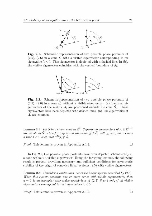
In Fig. 2.1, two possible phase portraits have been depicted schematically ina cone with a visible eigenvector. A similar result is obtained for trajectoriesinside cones, that do not contain visible eigenvectors.
2.3 Stability of an equilibrium at the bifurcation point 21
Fig. 2.1. Schematic representation of two possible phase portraits of(2.5), (2.6) in a cone Si with a visible eigenvector corresponding to aneigenvalue λ < 0. This eigenvector is depicted with a dashed line. In (b),the visible eigenvector coincides with the vertical boundary of Si.
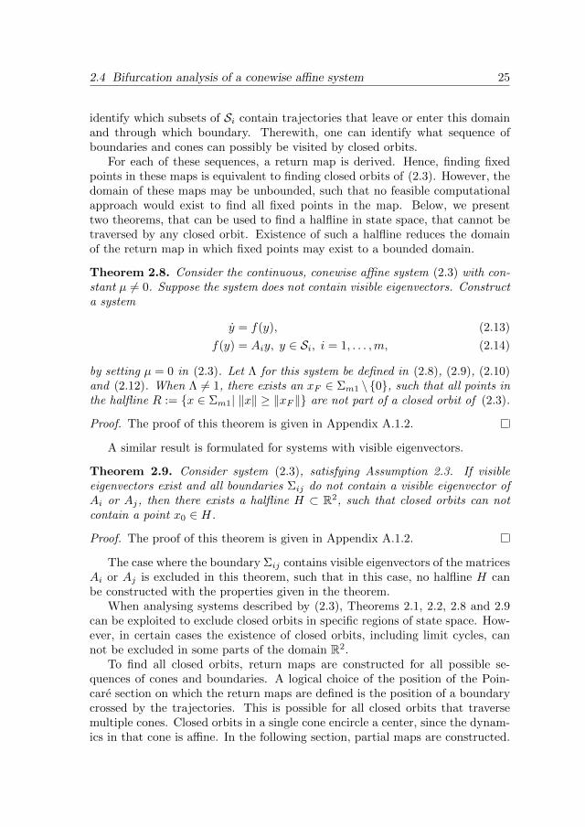
Fig. 2.2. Schematic representation of two possible phase portraits of(2.5), (2.6) in a cone Si without a visible eigenvector. (a) Two real ei-genvectors of the matrix Ai are positioned outside the cone Si. Theseeigenvectors have been depicted with dashed lines. (b) The eigenvalues ofAi are complex.
Lemma 2.4. Let S be a closed cone in R2. Suppose no eigenvectors of A ∈ R2×2
are visible in S. Then for any initial condition y0 ∈ S, with y0 6= 0, there existsa time t ≥ 0 such that eAty0 6∈ S.
Proof. This lemma is proven in Appendix A.1.2.
In Fig. 2.2, two possible phase portraits have been depicted schematically ina cone without a visible eigenvector. Using the foregoing lemmas, the followingresult is proven, providing necessary and sufficient conditions for asymptoticstability of the origin of conewise linear systems (2.5) with visible eigenvectors.
Lemma 2.5. Consider a continuous, conewise linear system described by (2.5).When this system contains one or more cones with visible eigenvectors, theny = 0 is an asymptotically stable equilibrium of (2.5) if and only if all visibleeigenvectors correspond to real eigenvalues λ < 0.
Proof. This lemma is proven in Appendix A.1.2.

22 Chapter 2. Bifurcations of equilibria in non-differentiable systems
Fig. 2.3. Illustration of a trajectory of (2.5) that traverses each coneSi, i = 1, . . . , 4, once per rotation.
2.3.2 Systems without visible eigenvectors
In conewise linear systems (2.5) without visible eigenvectors, trajectories exhibita spiralling motion around the origin, visiting each region Si, i = 1, . . . ,m, onceper rotation, as shown in Fig. 2.3. Stability results are obtained for the spirallingmotion by the computation of a return map.
In the absence of visible eigenvectors, a trajectory in the region Si, i =1, . . . ,m, will traverse this region in finite time, cf. Lemma 2.4. The position y0
where a trajectory enters this region at time t0 = 0 is located on the boundaryΣi−1,i, such that y0 can be expressed as y0 = piρi−1,i. Furthermore, this tra-jectory will cross Σi,i+1 in a finite time ti. The position of this crossing can begiven as: y(ti) = pi+1ρi,i+1. Since the dynamics inside the cone are linear, thetime ti can be solved for, such that y(ti) is parallel to ρi,i+1. In this manner,in [4], expressions for the traversal time and crossing positions are derived. Thecrossing positions are linear in pi. Using such analysis, we can derive expressionsfor a scalar Mi, such that pi+1 = Mip
i. Note, that similar expressions have beenderived in [4] for systems (2.5) with cones, that are convex.
First, the position vectors y and tangency vectors ρ are represented in a newcoordinate frame:
yi = P−1i y, for yi ∈ Si := yi ∈ R2|yi = P−1
i y, y ∈ Si, (2.7)
where Pi is given by the real Jordan decomposition of Ai, yielding Ai = PiJiP−1i .
This decomposition distinguishes three cases.
Case 1: If Ai has complex eigenvalues, then Ji =
[ai −ωiωi ai
], where ai and ωi
are real constants and ωi > 0. Define Ψ(a1, a2) to be the angle in anticlockwisedirection from vector a1 to vector a2. Herewith,
Mi =‖ρii−1,i‖‖ρii,i+1‖
eaiωi
Ψ(ρii−1,i,ρii,i+1)
. (2.8)

2.3 Stability of an equilibrium at the bifurcation point 23
Case 2: If Ai has two distinct real eigenvalues λai and λbi and two distinct
eigenvectors, then Ji =
[λai 00 λbi
]and
Mi =
∣∣∣∣∣eT2 ρii,i+1
eT2 ρii−1,i
∣∣∣∣∣λai
λbi−λai∣∣∣∣∣eT1 ρii,i+1
eT1 ρii−1,i
∣∣∣∣∣λbi
λai−λbi
, (2.9)
where e1 :=(1 0)T
and e2 :=(0 1)T
.Case 3: If Ai has two equal real eigenvalues λai with geometric multiplicity 1,
then Ji =
[λai 10 λai
]and
Mi =
∣∣∣∣∣eT2 ρii−1,i
eT2 ρii,i+1
∣∣∣∣∣ eλai(eT1 ρ
ii,i+1
eT2 ρii,i+1
−eT1 ρ
ii−1,i
eT2 ρii−1,i
). (2.10)
By computation of the scalars Mi with (2.8), (2.9) or (2.10) for each cone Si, i =1, . . . ,m, one can compute the return map between the positions yk and yk+1 oftwo subsequent crossings of the trajectory y(t) with the boundary Σm1:
yk+1 = Λyk, (2.11)
where
Λ =
m∏i=1
Mi. (2.12)
2.3.3 Stability result
Using the results given in Sections 2.3.1 and 2.3.2, we can derive necessaryand sufficient conditions for the global asymptotic stability of the origin of theconewise linear system (2.5).
Theorem 2.6. The origin of the continuous, conewise linear system (2.5) isglobally asymptotically stable if and only if
(i) in each cone Si, i = 1, . . . ,m, all visible eigenvectors are associated witheigenvalues λ < 0,
(ii) in case no visible eigenvectors exist, it holds that Λ < 1, with Λ defined in(2.8), (2.9), (2.10) and (2.12).
Proof. The proof of this theorem is given in Appendix A.1.2.

24 Chapter 2. Bifurcations of equilibria in non-differentiable systems
2.4 Bifurcation analysis of a conewise affine sys-tem
The limit sets that can occur in planar continuous systems are equilibria, closedorbits and homoclinic or heteroclinic orbits. To analyse the occurring bifurca-tions in (2.3), we are interested in characterisation of these limit sets, includingtheir local stability, for different values of the system parameter µ. The rela-tionship between these limit sets and the limit sets of (2.1) will be discussed inSection 2.5. The following assumption is adopted to study the conewise affinesystem (2.3).
Assumption 2.3. All matrices Ai, i = 1, . . .m, of (2.3) are invertible.
Note that this assumption implies that for given bifurcation parameter µ,all equilibrium points xeq(µ) of (2.3), that satisfy f(xeq(µ), µ) = 0, are isolated.Solutions of conewise affine systems as given in (2.3) scale linearly with thebifurcation parameter µ, as formalised in the following lemma.
Lemma 2.7. Consider two continuous conewise affine systems x = f(x) +µib, µi ∈ (0,∞), i = 1, 2, where f(·) is piecewise linear with cone-shaped regions.If φ1(t) is a solution of x = f(x) + µ1b, then φ2(t) = µ2
µ1φ1(t) is a solution of
x = f(x) + µ2b.
Proof. The proof is omitted for the sake of brevity and follows from the obser-vation that f(x) is homogeneous of degree 1.
From this lemma, we conclude that a complete bifurcation diagram can be ob-tained by finding all existing limit sets at an arbitrary negative, and an arbitrarypositive parameter µ, and at the bifurcation point with µ = 0. Subsequently,with Lemma 2.7, the limit sets for all parameters µ can be found. The conewiseaffine system (2.3) is conewise linear if µ = 0. The dynamical behaviour of (2.3)at µ = 0 has been analysed in the previous section.
In continuous, conewise affine systems with µ 6= 0, the trajectories are tan-gent to a specific boundary Σij at zero, one, or all points on this boundary.When, at this boundary, there exists an isolated point where the trajectoriesare tangent to the boundary, then such a point will be called a tangency pointand denoted with Tij . We determine all tangency points of the conewise affinesystem and compute trajectories in forward and backward time through thesetangency points and through the origin. When the vector f(x, µ) of (2.3) isparallel to a boundary at all points of this boundary, then a trajectory existsthat is parallel to the boundary.
In addition, when a node or saddle point exists, the stable and unstablemanifolds of this point are computed. Computation of this finite number oftrajectories yields insight in the possible behaviour of all trajectories. Withthese manifolds and trajectories, for each domain Si, i = 1, . . . ,m, we can
2.4 Bifurcation analysis of a conewise affine system 25
identify which subsets of Si contain trajectories that leave or enter this domainand through which boundary. Therewith, one can identify what sequence ofboundaries and cones can possibly be visited by closed orbits.
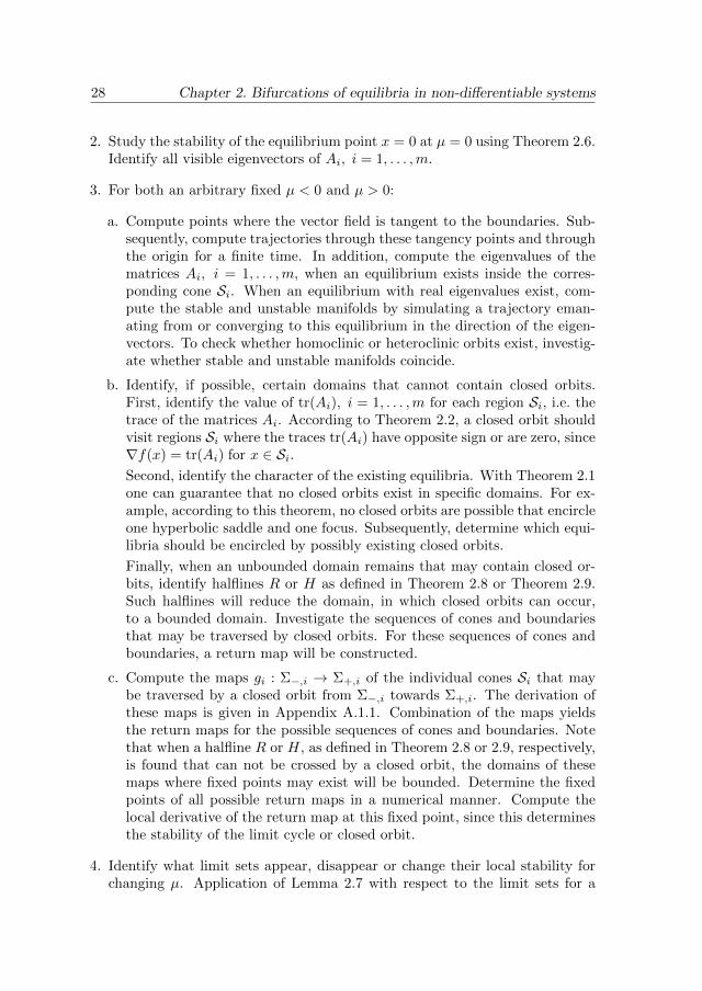
For each of these sequences, a return map is derived. Hence, finding fixedpoints in these maps is equivalent to finding closed orbits of (2.3). However, thedomain of these maps may be unbounded, such that no feasible computationalapproach would exist to find all fixed points in the map. Below, we presenttwo theorems, that can be used to find a halfline in state space, that cannot betraversed by any closed orbit. Existence of such a halfline reduces the domainof the return map in which fixed points may exist to a bounded domain.
Theorem 2.8. Consider the continuous, conewise affine system (2.3) with con-stant µ 6= 0. Suppose the system does not contain visible eigenvectors. Constructa system
y = f(y), (2.13)
f(y) = Aiy, y ∈ Si, i = 1, . . . ,m, (2.14)
by setting µ = 0 in (2.3). Let Λ for this system be defined in (2.8), (2.9), (2.10)and (2.12). When Λ 6= 1, there exists an xF ∈ Σm1 \ 0, such that all points inthe halfline R := x ∈ Σm1| ‖x‖ ≥ ‖xF ‖ are not part of a closed orbit of (2.3).
Proof. The proof of this theorem is given in Appendix A.1.2.
A similar result is formulated for systems with visible eigenvectors.
Theorem 2.9. Consider system (2.3), satisfying Assumption 2.3. If visibleeigenvectors exist and all boundaries Σij do not contain a visible eigenvector ofAi or Aj, then there exists a halfline H ⊂ R2, such that closed orbits can notcontain a point x0 ∈ H.
Proof. The proof of this theorem is given in Appendix A.1.2.
The case where the boundary Σij contains visible eigenvectors of the matricesAi or Aj is excluded in this theorem, such that in this case, no halfline H canbe constructed with the properties given in the theorem.
When analysing systems described by (2.3), Theorems 2.1, 2.2, 2.8 and 2.9can be exploited to exclude closed orbits in specific regions of state space. How-ever, in certain cases the existence of closed orbits, including limit cycles, cannot be excluded in some parts of the domain R2.
To find all closed orbits, return maps are constructed for all possible se-quences of cones and boundaries. A logical choice of the position of the Poin-care section on which the return maps are defined is the position of a boundarycrossed by the trajectories. This is possible for all closed orbits that traversemultiple cones. Closed orbits in a single cone encircle a center, since the dynam-ics in that cone is affine. In the following section, partial maps are constructed.

26 Chapter 2. Bifurcations of equilibria in non-differentiable systems
A partial map describes the position of a trajectory before and after the visit ofa specific cone Si, i = 1, . . . ,m. Subsequently, we discuss how to combine thesepartial maps to obtain the return map.
2.4.1 Trajectories visiting a cone SiIn Sections 2.3.1 and 2.3.2, a trajectory of a conewise linear system is followedinside a specific cone Si during the traversal of this cone. During this traversal,the trajectory is described by the linear differential equation y = Aiy, such thatan analytical expression for the trajectory y(t) with initial position y0 ∈ Σi−1,i
has been derived. With this expression, the traversal time ti and final positiony(ti) are obtained. Here, a similar approach is used for the conewise affinesystem (2.3), where we focus our attention on trajectories that traverse conesSi, i = 1, . . . ,m.
For a given cone Si, i = 1, . . . ,m, and given boundaries where the traject-ory enters or leaves this domain, the partial map is constructed that gives theexit position as a function of the position, where Si is entered. Since (2.3) isautonomous, we can assume without loss of generality that the domain Si isentered at the time t = 0. We study a trajectory traversing Si from the bound-ary Σ− towards the boundary Σ+ in a finite time ti. Therefore, the trajectoryx(t) satisfies x(t) ∈ Si, t ∈ (0, ti), x(0) ∈ Σ− and x(ti) ∈ Σ+. We define themaps gi : Di ⊂ Σ− → Ii ⊂ Σ+, describing the position x(ti) as a function ofx(0). Expressions for gi are derived in Appendix A.1.1.
2.4.2 Construction of the return map
The stable or unstable manifolds of nodes and saddle points and the trajectoriesthrough tangency points and the origin are computed. Therewith, for eachdomain Si, we can identify what subsets of Si contain trajectories that leave orenter this domain and through which boundary. Combining these domains, onecan identify what sequences of boundaries and cones can contain closed orbits.A return map is computed for each sequence to find all closed orbits and theirstability properties.
For example, suppose we want to study whether there exist one or moreclosed orbits that traverse the regions and boundaries S1,Σ12,S2,Σ23,S3,Σ31 inthis order. A Poincare section is taken at the moments where trajectories crossΣ31, the corresponding return map is denoted as M : DM ⊂ Σ31 → IM ⊂ Σ31.Therewith, M(xk) describes the first crossing of a trajectory x(t), t > 0 withboundary Σ31, where x(t) corresponds to the initial condition x(0) = xk ∈ DM .Define g1 : D1 ⊂ Σ31 → I1 ⊂ Σ12, which can be computed with Appendix A.1.1,where Σ− = Σ31 and Σ+ = Σ12. In addition, define g2 : D2 ⊂ Σ12 → I2 ⊂ Σ23
and g3 : D3 ⊂ Σ23 → I3 ⊂ Σ31 in a similar fashion. From a combination of g1,g2 and g3, one obtains the return map M(xk) = g3 g2 g1(xk).

2.4 Bifurcation analysis of a conewise affine system 27
Since M is a return map, every fixed point of this map is on a closed orbit.If this fixed point is isolated, then the periodic orbit is a limit cycle. Further-more, each closed orbit of (2.3) that traverses the boundaries and regions in thesequence S1,Σ12,S2,Σ23,S3,Σ31, yields a fixed point in M .
The return map M can be computed for the possible sequences of cones andboundaries. By determining the fixed points of such maps, the existence or ab-sence of limit cycles and closed orbits can be investigated. Each return map iscontinuous, since (2.3) is Lipschitz continuous, and trajectories of this class ofsystems are continuous with respect to initial conditions, see [91], Theorem 3.4.Furthermore, the Euclidean norm of the map, ‖M(x)‖, is monotonously increas-ing in ‖x‖. Monotonicity follows from the fact that the time-reversed system of(2.3) is Lipschitz as well, such that the inverse of M should exist and should beunique. The norm ‖M(x)‖ has to be increasing in ‖x‖. Otherwise, there wouldhave to exist points xa, xb ∈ DM , where ‖xa‖ < ‖xb‖ and ‖M(xa)‖ > ‖M(xb)‖.Note that M is a return map, such that there exist a trajectory from xa toM(xa) and a trajectory from xb towards M(xb). The positions xa, M(xa), xband M(xb) should all be positioned on the same boundary, that is a halfline. If‖xa‖ < ‖xb‖ and ‖M(xa)‖ > ‖M(xb)‖, in planar systems, the trajectories fromxa and xb have to cross each other before they return to the Poincare section.Such a crossing is not possible in systems that are Lipschitz. The fact thatthe return map is continuous and monotonously increasing can be used in thecomputational approach to find all fixed points.
2.4.3 Procedure to obtain all closed orbits
In this section, a stepwise procedure is developed such that all limit sets of (2.3)are found for negative, positive and zero bifurcation parameter µ. With thisprocedure, the bifurcations of the continuous, conewise affine system (2.3) canbe described entirely.
Lemma 2.7 implies that only an arbitrary positive and negative µ, and µ = 0,should be studied to obtain the full bifurcation diagram. Theorems 2.1 and 2.2are used to exclude the existence of closed orbits. For systems without visibleeigenvectors, Theorem 2.8 supplies a bound to exclude closed orbits far awayfrom the origin. If visible eigenvectors exist, Theorem 2.9 can be applied tobound the domain, in which closed orbits can occur. When Theorem 2.8 or2.9 can be applied, a bounded domain for the return map remains, such thatit is computationally feasible to find all fixed points of the return map with anumerical method. When certain sequences of boundaries and cones may containclosed orbits, return maps will be constructed.
The following procedure yields a bifurcation diagram of (2.3) that containsall limit sets:
1. Identify all equilibria for positive and negative µ, i.e. the points x ∈ R2 wheref(x, µ) = 0, with f(x, µ) given in (2.3).
28 Chapter 2. Bifurcations of equilibria in non-differentiable systems
2. Study the stability of the equilibrium point x = 0 at µ = 0 using Theorem 2.6.Identify all visible eigenvectors of Ai, i = 1, . . . ,m.
3. For both an arbitrary fixed µ < 0 and µ > 0:
a. Compute points where the vector field is tangent to the boundaries. Sub-sequently, compute trajectories through these tangency points and throughthe origin for a finite time. In addition, compute the eigenvalues of thematrices Ai, i = 1, . . . ,m, when an equilibrium exists inside the corres-ponding cone Si. When an equilibrium with real eigenvalues exist, com-pute the stable and unstable manifolds by simulating a trajectory eman-ating from or converging to this equilibrium in the direction of the eigen-vectors. To check whether homoclinic or heteroclinic orbits exist, investig-ate whether stable and unstable manifolds coincide.
b. Identify, if possible, certain domains that cannot contain closed orbits.First, identify the value of tr(Ai), i = 1, . . . ,m for each region Si, i.e. thetrace of the matrices Ai. According to Theorem 2.2, a closed orbit shouldvisit regions Si where the traces tr(Ai) have opposite sign or are zero, since∇f(x) = tr(Ai) for x ∈ Si.Second, identify the character of the existing equilibria. With Theorem 2.1one can guarantee that no closed orbits exist in specific domains. For ex-ample, according to this theorem, no closed orbits are possible that encircleone hyperbolic saddle and one focus. Subsequently, determine which equi-libria should be encircled by possibly existing closed orbits.
Finally, when an unbounded domain remains that may contain closed or-bits, identify halflines R or H as defined in Theorem 2.8 or Theorem 2.9.Such halflines will reduce the domain, in which closed orbits can occur,to a bounded domain. Investigate the sequences of cones and boundariesthat may be traversed by closed orbits. For these sequences of cones andboundaries, a return map will be constructed.
c. Compute the maps gi : Σ−,i → Σ+,i of the individual cones Si that maybe traversed by a closed orbit from Σ−,i towards Σ+,i. The derivation ofthese maps is given in Appendix A.1.1. Combination of the maps yieldsthe return maps for the possible sequences of cones and boundaries. Notethat when a halfline R or H, as defined in Theorem 2.8 or 2.9, respectively,is found that can not be crossed by a closed orbit, the domains of thesemaps where fixed points may exist will be bounded. Determine the fixedpoints of all possible return maps in a numerical manner. Compute thelocal derivative of the return map at this fixed point, since this determinesthe stability of the limit cycle or closed orbit.
4. Identify what limit sets appear, disappear or change their local stability forchanging µ. Application of Lemma 2.7 with respect to the limit sets for a

2.5 Approximation effects 29
given µ < 0 or µ > 0 yields all limit sets for µ 6= 0. Combination with thepiecewise linear stability result for the case µ = 0 gives a bifurcation diagram,containing all changes in limit sets and their stability.
The procedure given above yields all changes in the limit sets of the conewiseaffine system (2.3). Completeness of the obtained limit cycles follows from thefact that for each conewise affine system (2.3), a finite number of return mapscan be determined, that may contain fixed points. Computation of each of thesereturn maps yields all limit cycles.
2.5 Approximation effects
In this section, the effect of the conewise affine approximation of a non-differ-entiable system is studied, as introduced in Section 2.2. Results are presentedfor the existence and stability of equilibria (Theorem 2.10) and limit cycles(Theorem 2.11) in the non-differentiable system (2.1) when such limit sets existin the conewise affine system (2.3) and vise versa. With these theorems, weshow the applicability of the procedure for the bifurcation analysis as presentedin Section 2.4 for non-differentiable systems of the form (2.1).
We will use the following assumptions in addition to Assumptions 2.1 and2.2.
Assumption 2.4. For all functions Fi(x, ν), i = 1, . . . , m, the Jacobian at theorigin, i.e. ∂Fi
∂x
∣∣(x,ν)=(0,0)
, is invertible.
Note that this assumption is stricter than Assumption 2.3, in which only thevector fields Fi(x, ν), i = 1, . . . ,m, are considered. In a neighbourhood aroundthe origin, Assumption 2.4 excludes the existence of non-isolated equilibria indomains Di that are cusp-shaped at the origin.
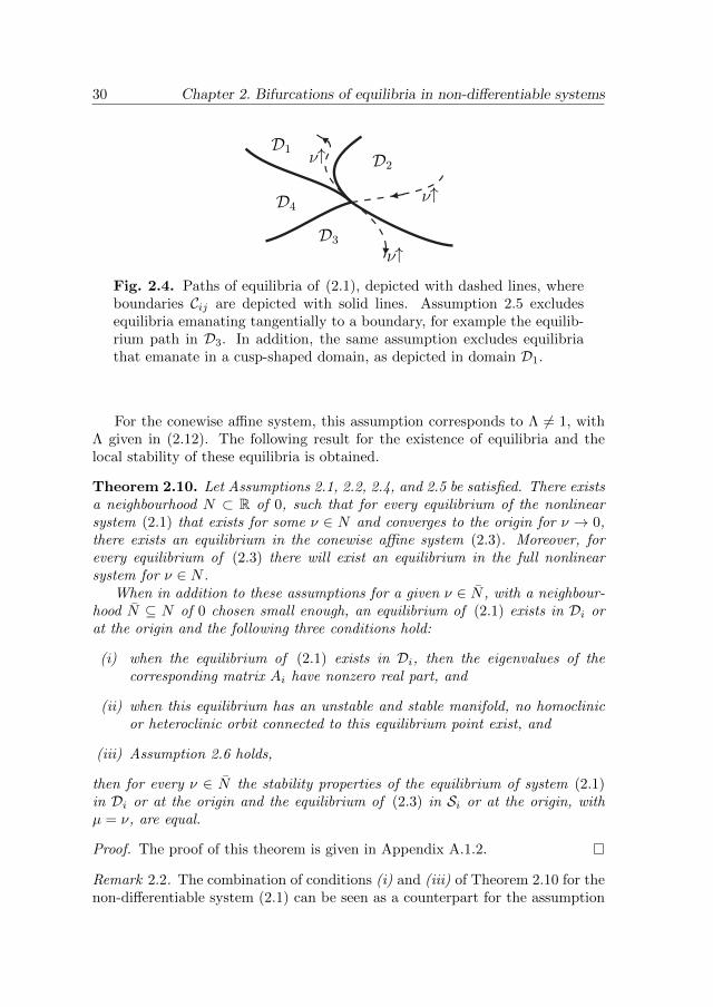
Assumption 2.5. The equilibria of the nonlinear system (2.1) do not movelocally tangential to the boundaries when ν is varied around 0.
We illustrate Assumption 2.5 in Fig. 2.4. This assumption implies thatnTi−1,iA
−1i b 6= 0,∀i ∈ 1, . . . ,m.
Remark 2.1. Paths of equilibria that approach the origin through a cusp-shapedregion are excluded by Assumption 2.5. C
Without loss of generality, we may assume that∥∥∥ ∂F∂ν ∣∣(x,ν)=(0,0)
∥∥∥ = 1, yielding
µ = ν. In the following assumption, the occurrence of center-like behaviour isexcluded.
Assumption 2.6. In a neighbourhood around the origin, the non-differentiablesystem (2.1) and conewise affine system (2.3) at the bifurcation point ν = 0or µ = 0 do not contain trajectories that are encircling the equilibrium withoutconverging to the origin for t→∞ or t→ −∞.
30 Chapter 2. Bifurcations of equilibria in non-differentiable systems
Fig. 2.4. Paths of equilibria of (2.1), depicted with dashed lines, whereboundaries Cij are depicted with solid lines. Assumption 2.5 excludesequilibria emanating tangentially to a boundary, for example the equilib-rium path in D3. In addition, the same assumption excludes equilibriathat emanate in a cusp-shaped domain, as depicted in domain D1.
For the conewise affine system, this assumption corresponds to Λ 6= 1, withΛ given in (2.12). The following result for the existence of equilibria and thelocal stability of these equilibria is obtained.
Theorem 2.10. Let Assumptions 2.1, 2.2, 2.4, and 2.5 be satisfied. There existsa neighbourhood N ⊂ R of 0, such that for every equilibrium of the nonlinearsystem (2.1) that exists for some ν ∈ N and converges to the origin for ν → 0,there exists an equilibrium in the conewise affine system (2.3). Moreover, forevery equilibrium of (2.3) there will exist an equilibrium in the full nonlinearsystem for ν ∈ N .
When in addition to these assumptions for a given ν ∈ N , with a neighbour-hood N ⊆ N of 0 chosen small enough, an equilibrium of (2.1) exists in Di orat the origin and the following three conditions hold:
(i) when the equilibrium of (2.1) exists in Di, then the eigenvalues of thecorresponding matrix Ai have nonzero real part, and
(ii) when this equilibrium has an unstable and stable manifold, no homoclinicor heteroclinic orbit connected to this equilibrium point exist, and
(iii) Assumption 2.6 holds,
then for every ν ∈ N the stability properties of the equilibrium of system (2.1)in Di or at the origin and the equilibrium of (2.3) in Si or at the origin, withµ = ν, are equal.
Proof. The proof of this theorem is given in Appendix A.1.2.
Remark 2.2. The combination of conditions (i) and (iii) of Theorem 2.10 for thenon-differentiable system (2.1) can be seen as a counterpart for the assumption
2.5 Approximation effects 31
of hyperbolic dynamics near equilibria of smooth systems, as would be requiredto apply the Hartman-Grobman Theorem, cf. [74]. C
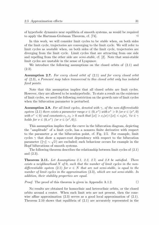
In this work, we will consider limit cycles to be stable when, on both sidesof the limit cycle, trajectories are converging to the limit cycle. We will refer tolimit cycles as unstable when, on both sides of the limit cycle, trajectories arediverging from the limit cycle. Limit cycles that are attracting from one sideand repelling from the other side are semi-stable, cf. [2]. Note that semi-stablelimit cycles are unstable in the sense of Lyapunov.
We introduce the following assumptions on the closed orbits of (2.1) and(2.3).
Assumption 2.7. For every closed orbit of (2.1) and for every closed orbitof (2.3), a Poincare map taken transversal to this closed orbit only has isolatedfixed points.
Note that this assumption implies that all closed orbits are limit cycles.However, they are allowed to be nonhyperbolic. To state a result on the existenceof limit cycles, we need the following restriction on the growth rate of limit cycleswhen the bifurcation parameter is perturbed.
Assumption 2.8. For all limit cycles, denoted with γ, of the non-differentiablesystem (2.1) there exists a parameter range ν ∈ (0, ν∗) with ν∗ > 0 (or ν ∈ (ν∗, 0)with ν∗ < 0) and constants c1, c2 > 0 such that ‖x‖ > c1|ν|∧‖x‖ < c2|ν|, ∀x ∈ γholds for ν ∈ (0, ν∗) (or ν ∈ (ν∗, 0)).
This assumption implies that the curve in the bifurcation diagram, depictingthe ”amplitude” of a limit cycle, has a nonzero finite derivative with respectto the parameter µ at the bifurcation point, cf. Fig. 2.5. For example, limitcycles γ that show a square-root dependency with respect to the bifurcationparameter (‖γ‖ ∼ √ν) are excluded; such behaviour occurs for example in theHopf bifurcations of smooth systems.
The following theorem describes the relationship between limit cycles of (2.1)and (2.3).
Theorem 2.11. Let Assumptions 2.1, 2.2, 2.7, and 2.8 be satisfied. Thereexists a neighbourhood N of 0, such that the number of limit cycles in the non-differentiable system (2.1) for ν ∈ N that are not semi-stable, is equal to thenumber of limit cycles in the approximation (2.3), which are not semi-stable. Inaddition, their stability properties are equal.
Proof. The proof of this theorem is given in Appendix A.1.2.
No results are obtained for homoclinic and heteroclinic orbits, or the closedorbits around a center. When such limit sets are not present, then the cone-wise affine approximation (2.3) serves as a good local approximation of (2.1).Theorem 2.10 shows that equilibria of (2.1) are accurately represented in the
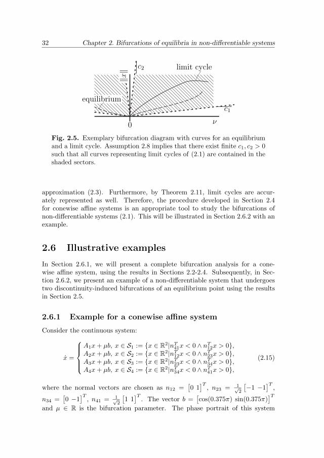
32 Chapter 2. Bifurcations of equilibria in non-differentiable systems
Fig. 2.5. Exemplary bifurcation diagram with curves for an equilibriumand a limit cycle. Assumption 2.8 implies that there exist finite c1, c2 > 0such that all curves representing limit cycles of (2.1) are contained in theshaded sectors.
approximation (2.3). Furthermore, by Theorem 2.11, limit cycles are accur-ately represented as well. Therefore, the procedure developed in Section 2.4for conewise affine systems is an appropriate tool to study the bifurcations ofnon-differentiable systems (2.1). This will be illustrated in Section 2.6.2 with anexample.
2.6 Illustrative examples
In Section 2.6.1, we will present a complete bifurcation analysis for a cone-wise affine system, using the results in Sections 2.2-2.4. Subsequently, in Sec-tion 2.6.2, we present an example of a non-differentiable system that undergoestwo discontinuity-induced bifurcations of an equilibrium point using the resultsin Section 2.5.
2.6.1 Example for a conewise affine system
Consider the continuous system:
x =
A1x+ µb, x ∈ S1 := x ∈ R2|nT41x < 0 ∧ nT12x > 0,A2x+ µb, x ∈ S2 := x ∈ R2|nT12x < 0 ∧ nT23x > 0,A3x+ µb, x ∈ S3 := x ∈ R2|nT23x < 0 ∧ nT34x > 0,A4x+ µb, x ∈ S4 := x ∈ R2|nT34x < 0 ∧ nT41x > 0,
(2.15)
where the normal vectors are chosen as n12 =[0 1]T
, n23 = 1√2
[−1 −1
]T,
n34 =[0 −1
]T, n41 = 1√
2
[1 1]T
. The vector b =[cos(0.375π) sin(0.375π)
]Tand µ ∈ R is the bifurcation parameter. The phase portrait of this system
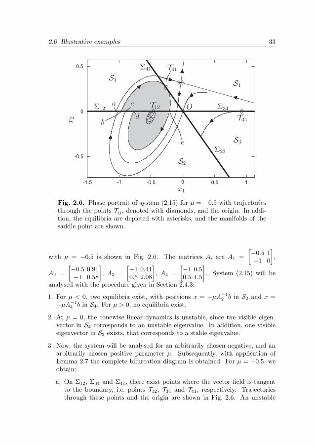
2.6 Illustrative examples 33
Fig. 2.6. Phase portrait of system (2.15) for µ = −0.5 with trajectoriesthrough the points Tij , denoted with diamonds, and the origin. In addi-tion, the equilibria are depicted with asterisks, and the manifolds of thesaddle point are shown.
with µ = −0.5 is shown in Fig. 2.6. The matrices Ai are A1 =
[−0.5 1−1 0
],
A2 =
[−0.5 0.91−1 0.58
], A3 =
[−1 0.410.5 2.08
], A4 =
[−1 0.50.5 1.5
]. System (2.15) will be
analysed with the procedure given in Section 2.4.3:
1. For µ < 0, two equilibria exist, with positions x = −µA−12 b in S2 and x =
−µA−14 b in S4. For µ > 0, no equilibria exist.
2. At µ = 0, the conewise linear dynamics is unstable, since the visible eigen-vector in S4 corresponds to an unstable eigenvalue. In addition, one visibleeigenvector in S3 exists, that corresponds to a stable eigenvalue.
3. Now, the system will be analysed for an arbitrarily chosen negative, and anarbitrarily chosen positive parameter µ. Subsequently, with application ofLemma 2.7 the complete bifurcation diagram is obtained. For µ = −0.5, weobtain:
a. On Σ12, Σ34 and Σ41, there exist points where the vector field is tangentto the boundary, i.e. points T12, T34 and T41, respectively. Trajectoriesthrough these points and the origin are shown in Fig. 2.6. An unstable

34 Chapter 2. Bifurcations of equilibria in non-differentiable systems
focus exist in S2, since the related eigenvalues of A2 are 0.42±0.79ı, whereı2 = −1. A saddle point exist in S4 with eigenvalues −1.10 and 1.60. Thestable and unstable manifolds of this point are shown and do not form ahomoclinic orbit.
b. The trace tr(A1) < 0, whereas all other traces satisfy tr(Ai) > 0, i = 2, 3, 4.Therefore, application of Theorem 2.2 yields that each possible closed orbitvisits S1. To satisfy Theorem 2.1, closed orbit(s) should encircle the focuswithout encircling the saddle point.
By studying the depicted trajectories, one can conclude, that no closedorbit can traverse Σ12 \ [O, a], since these trajectories cannot encircle thefocus without encircling the saddle point, which is required according toTheorem 2.1. Furthermore, closed orbits can not traverse the interior ofthe line [a, b], since trajectories through this open line will arrive at theline [c, d] in finite time, and enter the positively invariant region that isdepicted gray in Fig. 2.6. Now, one can conclude, that possible closedorbits visit only the regions S1 and S2, such that they should be containedin the domain, that is depicted gray. This implies, that all closed orbitstraverse the line [T12, e].
c. Existing closed orbits should traverse the line [T12, e]. We construct a mapg2 : [T12, e] → [d, T12], that yields the position g2(x) where a trajectoryleaves the cone S2 when this cone was entered at x. Similarly, the mapg1 : [b, T12] → [T12, e] is computed. The maps are computed as presentedin Appendix A.1.1. The combined map M := g1 g2(x) is the return mapand is shown in Fig. 2.7(a). It contains one fixed point. Apparently, a
unique stable limit cycle exists that contains x =(−0.55 0
)T.
For µ = 0.5, no equilibrium point of (2.15) exists, such that according toTheorem 2.1, no closed orbits can exist.
4. With the analysis above and application of Lemma 2.7, the bifurcation dia-gram is constructed, as given in Fig. 2.7(b). Both the limit cycle, focus andsaddle exist only for µ < 0. For µ = 0, unstable behaviour is observed. Wenote that this bifurcation can not occur in smooth dynamical systems and isexplicitly induced by the nonsmoothness of the system.
2.6.2 Example for a piecewise smooth system
In the following example, a piecewise smooth system is studied that under-goes two bifurcations of an equilibrium. Using the procedure presented in thischapter, a local analysis of these bifurcations is performed. For the conewiseaffine approximations, this analysis guarantees to find all equilibria and limitcycles that are created or destroyed locally during the bifurcations. According

2.6 Illustrative examples 35
Fig. 2.7. (a) Combined map M of (2.15) with µ = −0.5. (b) Bifurcationdiagram of (2.15) with the bifurcation parameter µ.
to Theorems 2.10 and 2.11, the local bifurcations of the piecewise smooth systemare accurately described.
We consider the following continuous piecewise smooth system:
x = Fi(x, ν), x ∈ Di, i = 1, 2, 3, (2.16)
where x =[x1 x2
]T ∈ R2, ν ∈ R is the bifurcation parameter and
F1(x, ν) =A1x+ νb+ 0.1
[0x3
1
], (2.17)
F2(x, ν) =A2x+ νb+ 0.1
[0x3
1
], (2.18)
F3(x, ν) =A3x+ νb, (2.19)
and A1 =
[0.5 −11 0
], A2 =
[0.5 −11 −0.75
], A3 =
[0.5 −1−0.5 0
]. The vector
b =[cos(0.375π) sin(0.375π)
]T. The domains Di, i = 1, 2, 3, are given by
D1 =x ∈ R2|nT31x < 0 ∧ nT12x > 0, (2.20)
D2 =x ∈ R2|nT12x < 0 ∨ h23(x) < 0, (2.21)
D3 =x ∈ R2|nT31x > 0 ∧ h23(x) > 0, (2.22)
where the function h23(x) is defined to describe the boundary between D2 andD3:
h23(x) := x2 −4
30x3
1 − 2x1, (2.23)
n31 =[1 0]T
and n12 =[0 1]T
. The boundary between Di and Dj is called Cij .The partitioning of the state space of this piecewise smooth system is depictedin Fig. 2.8(a).
First, we study at what parameters an equilibrium point is coinciding withone or more boundaries. An equilibrium point is positioned at the origin at
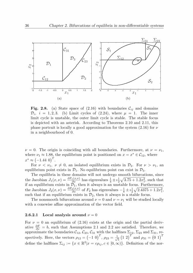
36 Chapter 2. Bifurcations of equilibria in non-differentiable systems
(a) (b)
Fig. 2.8. (a) State space of (2.16) with boundaries Cij and domainsDi, i = 1, 2, 3. (b) Limit cycles of (2.24), where µ = 1. The innerlimit cycle is unstable, the outer limit cycle is stable. The stable focusis depicted with an asterisk. According to Theorems 2.10 and 2.11, thisphase portrait is locally a good approximation for the system (2.16) for νin a neighbourhood of 0.
ν = 0. The origin is coinciding with all boundaries. Furthermore, at ν = ν1,where ν1 ≈ 1.88, the equilibrium point is positioned on x = x∗ ∈ C12, where
x∗ ≈(−1.44 0
)T.
For ν < ν1, ν 6= 0, an isolated equilibrium exists in D2. For ν > ν1, anequilibrium point exists in D1. No equilibrium point can exist in D3.
The equilibria in these domains will not undergo smooth bifurcations, since
the Jacobian J1(x, ν) = ∂F1(x,ν)∂x has eigenvalues 1
4 ± ı 12√
3.75 + 1.2x21, such that
if an equilibrium exists in D1, then it always is an unstable focus. Furthermore,
the Jacobian J2(x, ν) = ∂F2(x,ν)∂x of F2 has eigenvalues − 1
8 ± ı 12√
2.4375 + 1.2x21,
such that if an equilibrium exists in D2, then it always is a stable focus.The nonsmooth bifurcations around ν = 0 and ν = ν1 will be studied locally
with a conewise affine approximation of the vector field.
2.6.2.1 Local analysis around ν = 0
For ν = 0 an equilibrium of (2.16) exists at the origin and the partial deriv-ative ∂F
∂ν = b, such that Assumptions 2.1 and 2.2 are satisfied. Therefore, weapproximate the boundaries C12, C23, C31 with the halflines Σ12, Σ23 and Σ31, re-
spectively. Here, the vectors ρ12 =(−1 0
)T, ρ23 = 1√
5
(1 2)T
and ρ31 =(0 1)T
define the halflines Σij := x ∈ R2|x = cρij , c ∈ [0,∞). Definition of the nor-
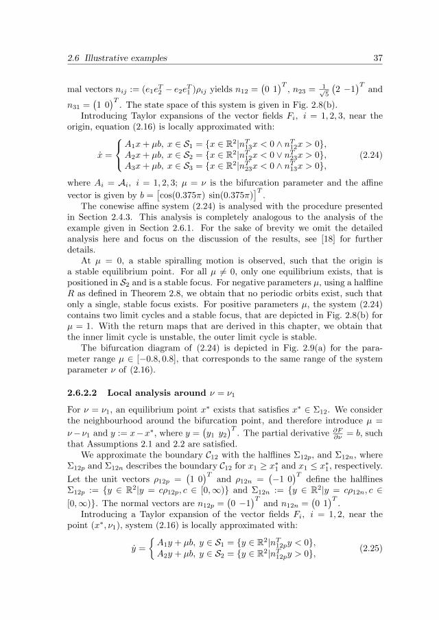
2.6 Illustrative examples 37
mal vectors nij := (e1eT2 − e2e
T1 )ρij yields n12 =
(0 1)T
, n23 = 1√5
(2 −1
)Tand
n31 =(1 0)T
. The state space of this system is given in Fig. 2.8(b).Introducing Taylor expansions of the vector fields Fi, i = 1, 2, 3, near the
origin, equation (2.16) is locally approximated with:
x =
A1x+ µb, x ∈ S1 = x ∈ R2|nT13x < 0 ∧ nT12x > 0,A2x+ µb, x ∈ S2 = x ∈ R2|nT12x < 0 ∨ nT23x > 0,A3x+ µb, x ∈ S3 = x ∈ R2|nT23x < 0 ∧ nT13x > 0,
(2.24)
where Ai = Ai, i = 1, 2, 3; µ = ν is the bifurcation parameter and the affine
vector is given by b =[cos(0.375π) sin(0.375π)
]T.
The conewise affine system (2.24) is analysed with the procedure presentedin Section 2.4.3. This analysis is completely analogous to the analysis of theexample given in Section 2.6.1. For the sake of brevity we omit the detailedanalysis here and focus on the discussion of the results, see [18] for furtherdetails.
At µ = 0, a stable spiralling motion is observed, such that the origin isa stable equilibrium point. For all µ 6= 0, only one equilibrium exists, that ispositioned in S2 and is a stable focus. For negative parameters µ, using a halflineR as defined in Theorem 2.8, we obtain that no periodic orbits exist, such thatonly a single, stable focus exists. For positive parameters µ, the system (2.24)contains two limit cycles and a stable focus, that are depicted in Fig. 2.8(b) forµ = 1. With the return maps that are derived in this chapter, we obtain thatthe inner limit cycle is unstable, the outer limit cycle is stable.
The bifurcation diagram of (2.24) is depicted in Fig. 2.9(a) for the para-meter range µ ∈ [−0.8, 0.8], that corresponds to the same range of the systemparameter ν of (2.16).
2.6.2.2 Local analysis around ν = ν1
For ν = ν1, an equilibrium point x∗ exists that satisfies x∗ ∈ Σ12. We considerthe neighbourhood around the bifurcation point, and therefore introduce µ =
ν−ν1 and y := x−x∗, where y =(y1 y2
)T. The partial derivative ∂F
∂ν = b, suchthat Assumptions 2.1 and 2.2 are satisfied.
We approximate the boundary C12 with the halflines Σ12p, and Σ12n, whereΣ12p and Σ12n describes the boundary C12 for x1 ≥ x∗1 and x1 ≤ x∗1, respectively.
Let the unit vectors ρ12p =(1 0)T
and ρ12n =(−1 0
)Tdefine the halflines
Σ12p := y ∈ R2|y = cρ12p, c ∈ [0,∞) and Σ12n := y ∈ R2|y = cρ12n, c ∈[0,∞). The normal vectors are n12p =
(0 −1
)Tand n12n =
(0 1)T
.Introducing a Taylor expansion of the vector fields Fi, i = 1, 2, near the
point (x∗, ν1), system (2.16) is locally approximated with:
y =
A1y + µb, y ∈ S1 = y ∈ R2|nT12py < 0,A2y + µb, y ∈ S2 = y ∈ R2|nT12py > 0, (2.25)

38 Chapter 2. Bifurcations of equilibria in non-differentiable systems
Fig. 2.9. Application of conewise affine approximations for the bifurc-ation analysis of (2.16). In panel (a), the limit sets are shown of theconewise affine approximations at ν = 0 and ν = ν1. In panel (b), theequilibrium path of (2.16) is shown, which is computed analytically. Fur-thermore, the limit cycles are computed by repeated application of theshooting method. Since the stable limit cycle grows in amplitude with in-creasing ν, the contents of panel (b) is repeated in panel (c) with a largery-scale.
where A1 =
(A1 +
(0 0
0.3(x∗1)2 0
))and A2 =
(A2 +
(0 0
0.3(x∗1)2 0
)), where
the affine vector is given by b =[cos(0.375π) sin(0.375π)
]Tand µ ∈ R is the
bifurcation parameter.
Once more, for details of the analysis of bifurcations of (2.25) using theprocedure of Section 2.4, we refer to [18]. Here we focus on discussing theresults. For µ < 0, one equilibrium point exists in S2, that is a stable focus.This focus is encircled by an unstable limit cycle, as depicted in Fig. 2.10 forµ = −1. At µ = 0, an expanding spiralling motion is observed around the origin,such that the equilibrium at the origin is unstable. For µ > 0, one equilibriumpoint exist in S2, and no limit cycles exist.
The bifurcation diagram is depicted in Fig. 2.9(a) for the parameter rangeµ ∈ [−0.8, 0.8], that corresponds to the range of the system parameters ν ∈

2.7 Conclusions 39
Fig. 2.10. Unstable limit cycle of (2.25) with µ = −1. The stable focusis depicted with an asterisk.
[1.08, 2.68] of system (2.16). This type of bifurcation was identified in [101] as adiscontinuous Hopf bifurcation.
2.6.2.3 Bifurcations of the non-differentiable system
The nonsmooth bifurcations around ν = 0 and ν = ν1 are approximated loc-ally in the previous sections, yielding the bifurcation diagram as depicted inFig. 2.9.a. According to Theorems 2.10 and 2.11, similar limit sets exist in thesmooth system (2.16). Using the approximations, the bifurcation diagram of(2.16) is given in Fig. 2.9.b and 2.9.c. The limit cycles created or destroyed bythe bifurcations, as found by the conewise affine approximations, are followedfor varying ν 6= 0 and ν 6= ν1 using a sequential implementation of the shootingalgorithm, cf. [129]. The path of the equilibrium point is computed analytically.
The local bifurcations of the equilibrium at ν = 0 and ν = ν1 are accur-ately described. However, since the conewise affine approximation uses a localapproximation of (2.16) near (ν, x) = (ν1, x
∗), the stable limit cycle induced atν = 0 is not identified by the local approximation around ν = ν1.
Note that the approach of this chapter does not yield information on bi-furcations of limit cycles. For example, with the presented analysis we can notexclude a bifurcation of the stable limit cycle for ν > 0.
2.7 Conclusions
A procedure is presented that yields a complete analysis of bifurcating equilib-ria in a class of hybrid systems, described by a continuous, piecewise smoothdifferential equations. This procedure is a computationally feasible method to

40 Chapter 2. Bifurcations of equilibria in non-differentiable systems
identify all limit sets that are created or destroyed during the bifurcation of anequilibrium point.
To analyse the bifurcation with the given procedure, under certain assump-tions, continuous, piecewise smooth hybrid systems can be approximated nearthe bifurcation point by a conewise affine system. The bifurcation of the ap-proximated, conewise affine system accurately describes the local bifurcation ofthe equilibrium point in the continuous, piecewise smooth system.
For the conewise affine system, we study what limit sets appear or disap-pear, change in character or in their stability properties under change of a sys-tem parameter. Existing equilibria, homoclinic and heteroclinic orbits of theconewise affine system can be found in a relatively straightforward manner. Theother limit sets that are possible in autonomous planar systems are closed orbits,including limit cycles. To find these, we study the Poincare return maps.
To be able to find all limit sets in a computationally feasible manner, newtheoretical results are presented. With these results, one can exclude the ex-istence of closed orbits far away from the equilibria. Using these theoreticalresults, the presented procedure is able to identify, in a computationally efficientmanner, all limit sets, which appear or disappear in the discontinuity-inducedbifurcation of the equilibrium of the approximated, conewise affine system. Theprocedure will identify all closed orbits, when multiple closed orbits are createdat the bifurcation point. In two examples, the theoretical results are illustrated.
The procedure presented in this chapter is useful to assess the parameterdependency of the dynamics of planar piecewise smooth systems. Knowledge onwhat limit sets can appear or disappear under parameter changes of a systemcan be useful in the design of a system that is non-differentiable, and can beused to evaluate the robustness of the system, which is generally an importantdesired characteristic for non-differentiable control systems.
The results of this work can be extended to a more general class of hybridsystems, described by piecewise smooth systems with a discontinuous right-hand side, which are relevant, for example, in the context of mechanical sys-tems with Coulomb friction. Analogue to the conewise affine approximation ofnon-differentiable systems, in the following chapter, we employ the linearisationof one smooth vector field near a discontinuity to study trajectories near equi-librium sets in discontinuous systems describing mechanical systems with dryfriction.

Chapter 3
Bifurcations of equilibrium sets inmechanical systems with dry
friction
Abstract – The presence of dry friction in mechanical systems induces the existence of an
equilibrium set, consisting of infinitely many equilibrium points. The local dynamics of the
trajectories near an equilibrium set is investigated for systems with one frictional interface. In
this case, the equilibrium set will be an interval of a curve in phase space. It is shown in this
chapter that local bifurcations of equilibrium sets occur near the endpoints of this curve. Based
on this result, sufficient conditions for structural stability of equilibrium sets in planar systems
are given and two new bifurcations are identified. The results are illustrated by application to
a controlled mechanical system with friction.
3.1 Introduction
Many mechanical systems experience stick due to dry friction, such that traject-ories converge to an equilibrium set, that consists of a continuum of equilibriumpoints, rather than to an isolated equilibrium point. Dry friction appears atvirtually all physical interfaces that are in contact. The presence of equilibriumsets in engineering systems compromises positioning accuracy in motion controlsystems, such as robot positioning control, see e.g. [115, 120, 133]. Dry frictionmay also cause other effects that deteriorate performance of motion control sys-tems, such as the occurrence of periodic orbits, cf. [79, 133]. In this chapter,sufficient conditions for structural stability of equilibrium sets are given, andbifurcations of equilibrium sets are studied.
This chapter is based on [26], and parts have appeared in [24,25].

42 Chapter 3. Bifurcations of equilibrium sets in mechanical systems
The dry friction force is modelled with a set-valued friction law that dependson the slip velocity, such that the friction law is set-valued only at zero slipvelocity. Using such a set-valued friction law, the systems are described by adifferential inclusion. Such friction laws can accurately describe the existence ofan equilibrium set, see e.g. [66, 104, 164]. This class of friction models containsthe models of Coulomb and Stribeck. Dynamic friction models as discussedin [125] are not considered, since these models increase the dimension of thephase space, such that the study of bifurcations becomes more involved. In thischapter, the dynamics of mechanical systems are studied where dry friction ispresent in one interface.
The equilibrium sets of systems with dry friction may be stable or unstablein the sense of Lyapunov. In addition, equilibrium sets may attract all nearbytrajectories in finite time, cf. [104]. A natural question is to ask how changesin system parameters may influence these properties. To answer this question,structural stability and bifurcations of equilibrium sets are studied.
For this purpose, the local phase portrait near an equilibrium set is studiedand possible bifurcations are identified. Under a non-degeneracy condition, thelocal dynamics is shown to be always structurally stable near the equilibriumset except for two specific points, namely, the endpoints of the equilibrium set.Hence, analysis of the trajectories near these points yields a categorisation ofthe bifurcations that are possible. In this manner, particularly, bifurcations ofequilibrium sets of planar systems are studied in this chapter.
Although quite some results exist on the asymptotic stability and attractiv-ity of equilibrium sets of mechanical systems with dry friction, see [1, 39, 85,104,105,159], few results exist that describe bifurcations of equilibrium sets, seee.g. [86, 163]. In [104, 105, 159], Leine and van de Wouw derive sufficient condi-tions for attractivity and asymptotic stability of equilibrium sets using Lyapunovtheory and invariance results. In the papers of Adly, Attouch and Cabot [1,39],conditions are presented under which trajectories converge to the equilibrium setin finite time. Using Lyapunov functions, the attractive properties of individualpoints in the equilibrium sets are analysed in [85]. Existing results on bifurca-tions of systems with dry friction are either obtained using the specific propertiesof a given model, or they do not consider trajectories in the neighbourhood ofan equilibrium set. In [163], a van der Pol system is studied that experiencesCoulomb friction. By constructing a Poincare return map, Yabuno et al. showthat the limit cycle, created by a Poincare-Andronov-Hopf bifurcation for thesystem without friction, can not be created near the equilibrium set in the pres-ence of friction. In [86], the appearance or disappearance of an equilibrium setis studied by solving an algebraic inclusion.
Bifurcations of the larger family of differential inclusions, that contains mod-els of mechanical systems with friction, are studied e.g. in [15,16,47,58,71,94,96,101, 103, 151]. Bifurcations of limit cycles of discontinuous systems are studiedusing a return map, see [15, 47, 94, 103]. However, in these systems the fric-

3.2 Modelling and main result 43
tion interface is moving, such that the discontinuity surface does not containequilibria. Bifurcations of equilibria in two- or three-dimensions are studied ine.g. [16, 58, 96, 151]. Here, the dynamics is understood by following the traject-ories that become tangent to a discontinuity boundary. Guardia et al. presentin [71] a generic classification of bifurcations with codimension one and two inplanar differential inclusions. However, the special structure of differential in-clusions describing mechanical systems with dry friction, which we will analysein this chapter, is considered to be non-generic by Guardia et al.. In the classof systems studied in this chapter, equilibrium sets occur generically, and per-sist when physically relevant perturbations are applied. Due to the difference inallowed perturbations, the scenarios observed in this chapter are not consideredin [71]. In [15, 101], the authors study bifurcations of equilibria in continuoussystems, that are not differentiable. Due to the assumptions posed in thesepapers, all equilibria are isolated points.
In this chapter, a more general class of mechanical systems with friction isstudied. Both the existence of an equilibrium set and the local phase portraitare investigated. Sufficient conditions for structural stability of this phase por-trait are given. Such conditions are derived for equilibrium points in smoothsystems, among others, by Hirsch, Smale, Hartman, and Pugh, see [74, 82, 132].Parallel to their approach in smooth systems, we analyse the structural stabilityof differential inclusions restricted to a neighbourhood of the equilibrium set. Atsystem parameters where the conditions for structural stability are not satisfied,two bifurcations are identified that do not occur in smooth systems.
The outline of this chapter is as follows. First, we introduce a model of amechanical system with friction in Section 3.2 and present the main result. Thistheorem states that local bifurcations of equilibrium sets occur in the neighbour-hood of two specific points, which are the endpoints of the equilibrium set. InSection 3.3, classes of systems are identified that are structurally stable. In Sec-tion 3.4, two bifurcations of the equilibrium set of planar systems are presented.In addition, it is shown that no limit cycles can be created by a local scenariosimilar to the Poincare-Andronov-Hopf bifurcation. In Section 3.5, the resultsof this chapter are illustrated with an example of a controlled mechanical sys-tem with dry friction. Conclusions are given in Section 3.6. In Section 3.7, wepresent an additional discussion on the relation to and differences with existingresults in the literature on bifurcations of discontinuous systems.
3.2 Modelling and main result
Consider a mechanical system that experiences friction on one interface betweentwo surfaces that move relative to each other in a given direction. Let x denotethe displacement in this direction and x denote the slip velocity, see Fig. 3.1 foran example. For an n−dimensional dynamical system this implies that n − 2other states y are required besides x and x. These states contain the other

44 Chapter 3. Bifurcations of equilibrium sets in mechanical systems
M2M1
−Fs Sign(x)
xy1
Fig. 3.1. Mechanical system subject to dry friction.
positions and velocities of the mechanical system, and, for example, controllerand observer states in the case of a feedback-controlled motion system. The
system given in Fig. 3.1 can be modelled with the additional states y =
(y1
y1
). In
general, using the states x, x and y, the dynamics are described by the followingdifferential inclusion, cf. [58]:
x− f(x, x, y) ∈ −Fs Sign(x),y = g(x, x, y),
(3.1)
where f and g are sufficiently smooth, Fs 6= 0, and Sign(·) denotes the set-valued
sign function Sign(p) =
p|p| , p 6= 0,
[−1, 1], p = 0.Note that (3.1) also encompasses systems with other nonlinearities than dry
friction, e.g. robotic systems. Introducing the state variables q =(x x yT
)T,
the dynamics of (3.1) can be reformulated as:
q ∈ F (q), (3.2)
F (q) =
F1(q), q ∈ S1 := q ∈ Rn : h(q) < 0,F2(q), q ∈ S2 := q ∈ Rn : h(q) > 0,coF1(q), F2(q), q ∈ Σ := q ∈ Rn : h(q) = 0,
(3.3)
where q ∈ Rn, co(a, b) denotes the smallest convex hull containing a and b, andF1, F2 and h are given by the smooth functions:
F1(q) =
xf(x, x, y) + Fsg(x, x, y)
; F2(q) =
xf(x, x, y)− Fsg(x, x, y)
; h(q) = x. (3.4)
In most existing bifurcation results for differential inclusions, see e.g. [16,58,96,151], parameter changes are considered that induce perturbations of the functionF in (3.2). Hence, in these studies the first component of F is perturbed, whichimplies that the case where the discontinuity surface coincides with the set where
3.2 Modelling and main result 45
the first element of F is zero is considered non-generic by these authors. Thisimplies that the existence of an equilibrium set in (3.2) is non-generic. However,parameter changes for the specific system (3.1) will only yield perturbations off and g in (3.2). Namely, for such mechanical systems, the perturbation ofthe kinematic relationship between position and velocity is not realistic. Usingthis insight, we show that for the class of systems under study, i.e. mechanicalsystems with set-valued friction, equilibrium sets will occur, generically.
To study trajectories at the discontinuity surface Σ, the solution concept ofFilippov is used, see [58]. Three domains are distinguished on the discontinuitysurface. If trajectories on both sides arrive at the boundary, then we have astable sliding region Σs. If one side of the boundary has trajectories towards theboundary, and trajectories on the other side leave the boundary, this domain iscalled the crossing region Σc (or transversal intersection). Otherwise, we havethe unstable sliding motion on the domain Σu. The mentioned domains areidentified as follows:
Σ : = q ∈ Rn : h(q) = 0Σs : = q ∈ Σ : LF1h > 0 ∧ LF2h < 0,Σu : = q ∈ Σ : LF1
h < 0 ∧ LF2h > 0,
Σc : = q ∈ Σ : (LF1h)(LF2
h) > 0,(3.5)
where LFih, i = 1, 2, denotes the directional derivative of h with respect to Fi,i.e. LFih = ∇hFi(q).
The vector field q = F s(q), that is active during sliding motion for q ∈Σu∪Σs, is defined by employing Filippov’s solution concept as follows. For eachq, the vector F s(q) is the vector on the segment between F1(q) and F2(q) thatis tangent to Σ at q:
q = F s(q) :=LF1
h(q)F2(q)− LF2h(q)F1(q)
LF1h(q)− LF2h(q)=
00
g(x, 0, y)
. (3.6)
Since LF1h = LF2
h + 2Fs, it follows from (3.5) that Fs > 0 implies that nounstable sliding occurs, and Fs < 0 implies that no stable sliding occurs. Theresulting phase space is shown schematically in Fig. 3.2 for the case n = 3.
In Lemma A.7, which is presented in Appendix A.2.1, we show that theequilibrium set is a segment of a curve on the discontinuity surface Σ when thefollowing assumption is satisfied.
Assumption 3.1. The functions f and g are such that
f(0, 0, 0) = 0, g(0, 0, 0) = 0 and
(∂f(x,0,y)
∂x∂f(x,0,y)
∂y∂g(x,0,y)
∂x∂g(x,0,y)
∂y
)is invertible for all (x, y) ∈
R× Rn−2. Furthermore, the map
(fg
)is proper1.
1A continuous map is proper if the inverse image of any compact set is compact.

46 Chapter 3. Bifurcations of equilibrium sets in mechanical systems
Fig. 3.2. Sketch of discontinuity surface Σ of (3.2)-(3.4) with n = 3 andFs > 0, containing an equilibrium set E .
For systems satisfying this assumption, the equilibrium set E of (3.1) is a one-dimensional curve as shown in Fig. 3.2. The equilibrium set of a differential in-clusion is given by 0 ∈ F (q), which is equivalent with (q ∈ Σs∪Σu∧LF2
hF1(q)−LF1
hF2(q) = 0), since 0 ∈(
q2
cof(q)− Fs, f(q) + Fs
)is equivalent with q ∈
Σs ∩ Σu and g(q) = 0 is equivalent with LF2hF1(q) − LF1
hF2(q) = 0 forq ∈ Σs ∩ Σu, see (3.6).
The equilibrium set is divided into interior points and the two endpoints asfollows:
E : = q ∈ Σu ∪ Σs : LF2hF1 − LF1hF2 = 0,I : = q ∈ E : F1 6= 0 ∧ F2 6= 0,Ei : = q ∈ E : Fi = 0, i = 1, 2.
(3.7)
Note that interior points are called pseudo-equilibria in [15]. The endpoints E1
and E2 satisfy LF1h = 0 or LF2
h = 0, respectively, hence they are positioned onthe boundary of the stable or unstable sliding mode as given by (3.5).
In this chapter, the trajectories near the equilibrium set will be studied. Theinfluence of perturbations of (3.1) on the phase portrait of a system is studied.For this purpose, we define the topological equivalence of phase portraits of(3.1) in Definition 3.1. We note that this definition is equal to the definition forsmooth systems, see e.g. [6, 32,72].
Definition 3.1 ([58]). We say that two dynamical systems in open domainsG1 and G2, respectively, are topologically equivalent if there exists a homeo-morphism from G1 to G2 which carries, as does its inverse, trajectories intotrajectories.
This equivalence relation allows for a homeomorphism that does not pre-serve the parameterisation of the trajectory with time, as required for topolo-gical conjugacy defined in [72]. Throughout this chapter, we assume that f andg smoothly depend on system parameters. When a parameter variation of a

3.3 Structural stability of the system near the equilibrium set 47
dynamical system A yields a system A which is not topologically equivalent toA, then the dynamical system experiences a bifurcation.
With the definitions given above, we can formulate our main result in thefollowing theorem.
Theorem 3.1. Assume (3.1) satisfies Assumption 3.1. If ∂g∂y
∣∣∣p
has no eigen-
value λ with real(λ) = 0 for any p ∈ E, then the dynamical system (3.1), in aneighbourhood of the equilibrium set, can only experience bifurcations near theendpoints E1 or E2.
Proof. The proof is given in Appendix A.2.2.
In the next section, we will first introduce the concept of structural stabil-ity, which is used in the proof of Theorem 3.1. We will employ a structuralstability definition that is tailored to systems of the form (3.1) and differs fromthe commonly used notion of structural stability for generic systems of the form(3.2). In particular, only perturbations on the right-hand side of (3.1) shouldbe considered. Subsequently, we will discuss the similarities between the line ofreasoning used in the proof of Theorem 3.1 and the standard arguments thatprove structural stability of hyperbolic equilibrium points in smooth systems.
3.3 Structural stability of the system near theequilibrium set
To prove Theorem 3.1, the influence of perturbations on systems (3.1) are stud-ied. If perturbations of f and g of (3.1) can not yield a dynamical system whichis not topologically equivalent to the original system, then the occurrence of bi-furcations is excluded. Hence, structural stability of (3.1) is investigated, whichis defined as follows.
Definition 3.2. A system A given by (3.1) is structurally stable for perturba-tions in f and g if there exists an ε > 0 such that the system A given by (3.1)with f and g such that
|f − f | < ε,
∥∥∥∥∥∂(f − f)
∂q
∥∥∥∥∥ < ε, ‖g − g‖ < ε,
∥∥∥∥∂(g − g)
∂q
∥∥∥∥ < ε, (3.8)
is topologically equivalent to system A.
Note, that this definition corresponds to C1-structural stability as definedby [146], and is tailored to dynamical systems described using second-order timederivatives of the state x.
Note that perturbations of (3.1) in f and g do not cause perturbations ofthe first component of F (·) in (3.2), as observed e.g. in [146] or [58, page 226].

48 Chapter 3. Bifurcations of equilibrium sets in mechanical systems
One consequence of this fact is that equilibrium sets occur generically in sys-tems (3.1), although they are non-generic in systems (3.2). In experiments onmechanical systems with dry friction, such equilibrium sets are found to occurgenerically, see e.g. [125]. For this reason, perturbations of the class (3.8) areused throughout this chapter. System A can be structurally stable for perturb-ations in f and g, whereas the corresponding system (3.2) is not structurallystable for general perturbations of F . Small changes of system parameters causesmall perturbations of f and g and their derivatives. However, the first equationof (3.2) will not change under parameter changes. Namely, this equation rep-resents the kinematic relationship between position and velocity of a mechanicalsystem, such that perturbation of this equation does not make sense for the classof physical systems under study. Hence, structural stability for perturbationsin f and g excludes the occurrence of bifurcations near the system parametersstudied.
In smooth systems, structural stability of dynamical systems in the neigh-bourhood of equilibrium points is studied four decades ago by, among others,Hirsch, Smale, Hartman, Grobman, and Pugh, see [74, 82, 132]. It is now wellknown that, restricted to the neighbourhood of an equilibrium point, smooth dy-namical systems are structurally stable when the equilibrium point is hyperbolic.For hyperbolic equilibrium points of smooth systems, the inverse function the-orem implies that the equilibrium point is translated over a small distance whenthe vector field is perturbed, and the perturbed vector field near this equilibriumpoint is ’close’ to the original vector field near the unperturbed equilibrium.Hence, the Hartman-Grobman theorem shows that there exists a topologicalequivalence for the phase portrait in the neighbourhoods of both equilibria. Inthis chapter, the structural stability of system (3.1) in the neighbourhood ofequilibrium sets is studied analogously.
Small perturbations of system (3.1) will cause the equilibrium set E to deform,but the equilibrium set of the perturbed system remains a smooth curve in statespace. Hence, there exists a smooth coordinate transformation (analogous tothe translation for smooth systems) that transforms the original equilibrium setE to the equilibrium set of the perturbed system, as shown in Appendix A.2.1.Furthermore, the vector field near both equilibrium sets are ’close’, as shown inLemma A.10. Using this coordinate transformation, Theorem 3.1 is be provenin Appendix A.2.2.
3.3.1 Structural stability of planar systems
In this section, sufficient conditions are presented for the structural stability ofplanar systems restricted to a neighbourhood of equilibrium sets, which form anextension of the conditions presented in Theorem 3.1. In the planar case, (3.1)and (3.2) reduce to, respectively:
x− f(x, x) ∈ −Fs Sign(x), (3.9)
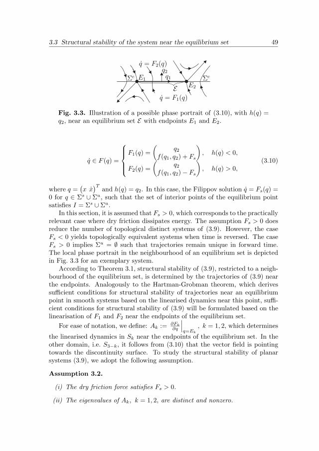
3.3 Structural stability of the system near the equilibrium set 49
Fig. 3.3. Illustration of a possible phase portrait of (3.10), with h(q) =q2, near an equilibrium set E with endpoints E1 and E2.
q ∈ F (q) =
F1(q) =
(q2
f(q1, q2) + Fs
), h(q) < 0,
F2(q) =
(q2
f(q1, q2)− Fs
), h(q) > 0,
(3.10)
where q =(x x)T
and h(q) = q2. In this case, the Filippov solution q = Fs(q) =0 for q ∈ Σs ∪ Σu, such that the set of interior points of the equilibrium pointsatisfies I = Σs ∪ Σu.
In this section, it is assumed that Fs > 0, which corresponds to the practicallyrelevant case where dry friction dissipates energy. The assumption Fs > 0 doesreduce the number of topological distinct systems of (3.9). However, the caseFs < 0 yields topologically equivalent systems when time is reversed. The caseFs > 0 implies Σu = ∅ such that trajectories remain unique in forward time.The local phase portrait in the neighbourhood of an equilibrium set is depictedin Fig. 3.3 for an exemplary system.
According to Theorem 3.1, structural stability of (3.9), restricted to a neigh-bourhood of the equilibrium set, is determined by the trajectories of (3.9) nearthe endpoints. Analogously to the Hartman-Grobman theorem, which derivessufficient conditions for structural stability of trajectories near an equilibriumpoint in smooth systems based on the linearised dynamics near this point, suffi-cient conditions for structural stability of (3.9) will be formulated based on thelinearisation of F1 and F2 near the endpoints of the equilibrium set.
For ease of notation, we define: Ak := ∂Fk∂q
∣∣∣q=Ek
, k = 1, 2, which determines
the linearised dynamics in Sk near the endpoints of the equilibrium set. In theother domain, i.e. S3−k, it follows from (3.10) that the vector field is pointingtowards the discontinuity surface. To study the structural stability of planarsystems (3.9), we adopt the following assumption.
Assumption 3.2.
(i) The dry friction force satisfies Fs > 0.
(ii) The eigenvalues of Ak, k = 1, 2, are distinct and nonzero.
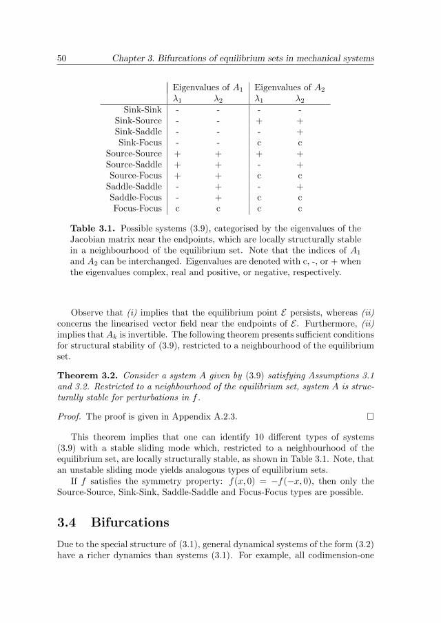
50 Chapter 3. Bifurcations of equilibrium sets in mechanical systems
Eigenvalues of A1 Eigenvalues of A2
λ1 λ2 λ1 λ2
Sink-Sink - - - -Sink-Source - - + +Sink-Saddle - - - +Sink-Focus - - c c
Source-Source + + + +Source-Saddle + + - +Source-Focus + + c c
Saddle-Saddle - + - +Saddle-Focus - + c cFocus-Focus c c c c
Table 3.1. Possible systems (3.9), categorised by the eigenvalues of theJacobian matrix near the endpoints, which are locally structurally stablein a neighbourhood of the equilibrium set. Note that the indices of A1
and A2 can be interchanged. Eigenvalues are denoted with c, -, or + whenthe eigenvalues complex, real and positive, or negative, respectively.
Observe that (i) implies that the equilibrium point E persists, whereas (ii)concerns the linearised vector field near the endpoints of E . Furthermore, (ii)implies that Ak is invertible. The following theorem presents sufficient conditionsfor structural stability of (3.9), restricted to a neighbourhood of the equilibriumset.
Theorem 3.2. Consider a system A given by (3.9) satisfying Assumptions 3.1and 3.2. Restricted to a neighbourhood of the equilibrium set, system A is struc-turally stable for perturbations in f .
Proof. The proof is given in Appendix A.2.3.
This theorem implies that one can identify 10 different types of systems(3.9) with a stable sliding mode which, restricted to a neighbourhood of theequilibrium set, are locally structurally stable, as shown in Table 3.1. Note, thatan unstable sliding mode yields analogous types of equilibrium sets.
If f satisfies the symmetry property: f(x, 0) = −f(−x, 0), then only theSource-Source, Sink-Sink, Saddle-Saddle and Focus-Focus types are possible.
3.4 Bifurcations
Due to the special structure of (3.1), general dynamical systems of the form (3.2)have a richer dynamics than systems (3.1). For example, all codimension-one
3.4 Bifurcations 51
bifurcations of (3.2) as observed in [96] can not occur in (3.1). In general, thesliding motion of the system (3.2) yields a nonzero sliding vector field, whereasthe sliding motion of (3.1) contains a set of equilibria. Therefore, in this sectionbifurcations of (3.1) are studied, restricting ourselves to planar systems as givenin (3.9). Such bifurcations occur in systems (3.2) as well, but will have a highercodimension.
Using Assumption 3.2, in Section 3.3 several types of topologically distinctplanar systems (3.9) are identified, which are structurally stable in a neigh-bourhood of the equilibrium set. Hence, it seems a reasonable step to considerparameter-dependent systems and study the parameters where the given con-ditions on the differential inclusion (3.9) no longer hold. In this manner, twobifurcations of planar systems (3.1) are presented. At the bifurcations points,Assumption 3.2.(ii) is violated.
3.4.1 Real or complex eigenvalues
Consider system (3.9) where eigenvalues of A1 change from real to complex eigen-
values under a parameter variation. From (3.9) it follows that A1 =
(0 1a21 a22
),
hence the eigenvalues of A1 are distinct when a21 6= − 14a
222 and the eigen-
values are both nonzero given a21 6= 0. Now, let the first part of Assump-tion 3.2(ii) be violated, such that the eigenvalues are equal. In that case, weobtain a21 = − 1
4a222.
Arbitrarily small variations of the system parameter a21 near a21 = − 14a
222
can create topologically distinct systems, since a system where A1 has complexeigenvalues is topologically distinct from a system where A1 has real eigenvalues.This follows from the observation that there exists a stable or unstable manifoldcontaining E1 if and only if A1 has real eigenvalues. Namely, there can notexist a homeomorphism that satisfies the conditions in Definition 3.1 and mapsa trajectory on this manifold to a trajectory of a system where A1 has complexeigenvalues, since in that case only one trajectory converges towards E1, whichoriginates from S2.
This bifurcation is illustrated with the following exemplary system:
x− a21x− a22x ∈ −Fs Sign(x), (3.11)
with Fs = 1, a22 = −0.1 and varying a21. In this example, the matrices A1
and A2 are equal, such that both endpoints undergo a bifurcation at the sametime. This system shows a bifurcation when a21 = −0.0025, as shown in Fig. 3.4.We refer to this bifurcation as a focus-node bifurcation. According to [39], alltrajectories of system (3.11) will arrive in the equilibrium set E in finite timeif and only if a21 < − 1
4a222 = −0.0025. For a21 ≥ 0.0025, the matrices A1
and A2 have a real eigenvector corresponding to an eigenvalue λ. The span ofthis eigenvector contains trajectories that converge exponentially according to

52 Chapter 3. Bifurcations of equilibrium sets in mechanical systems
−2000 −1000 0 1000−50
0
50
x
x
(a) a21 = −0.001
−2000 −1000 0 1000−50
0
50
xx
(b) a21 = −0.0025
−2000 −1000 0 1000−50
0
50
x
x
(c) a21 = −0.004
Fig. 3.4. System (3.11) with Fs = 1 and a22 = −0.1 showing a focus-node bifurcation. The equilibrium set E is given by a bold line, the realeigenvectors of the stable eigenvalues of A are represented with dashedlines. The real eigenvectors are distinct for a21 > −0.0025, collide at a21
and subsequently become imaginary.
x(t) − Ei = eλt(x(0) − Ei), i = 1, 2, which consequently does not converge infinite time. Hence, this change of the attractivity properties of the equilibriumset coincides with a bifurcation, defined using topological equivalence as used inthis chapter, see Definition 3.1.
3.4.2 Zero eigenvalue
Consider system (3.9) where an eigenvalue of A1 becomes zero under parameter
variation, where A1 =
(0 1a21 a22
). This matrix has an eigenvalue equal to zero
when a21 = 0 becomes zero.At the point E1 of the equilibrium set, the vector field satisfies F1(E1) = 0.
By definition, the point E1 is an endpoint of E , such that trajectories cross Σoutside E . This implies that the second component of F1, denoted F x1 , evaluatedon the curve Σ changes sign at E1. Since F1 is smooth and F x1 changes sign
at E1, we obtain∂kFx1∂xk
∣∣∣E1
6= 0 for an odd integer k ≥ 3, and∂iFx1∂xi
∣∣∣E1
= 0, for
i = 1, . . . , k − 1. The equilibrium set E on Σ is given by F x2 ≤ 0 and F x1 ≥ 0.A change of a system parameter can create two distinct domains where F x1 ≥ 0near E1, such that two equilibrium sets are created.
This bifurcation is illustrated with the following exemplary system:
x− a21x− a22x+ Fs + x3 ∈ −Fs Sign(x), (3.12)
with Fs = 1, a22 = −1 and varying a21. The system is designed such that theorigin is always the endpoint of an equilibrium set. The resulting phase portrait

3.4 Bifurcations 53
−1 −0.5 0 0.5−0.5
0
0.5
1
x
x
(a) a21 = −0.1
−1 −0.5 0 0.5−0.5
0
0.5
1
x
x(b) a21 = 0
−1 −0.5 0 0.5−0.5
0
0.5
1
x
x
(c) a21 = 0.1
Fig. 3.5. System (3.12) with Fs = 1, a22 = −1 and varying a21, showinga bifurcation where an eigenvalue becomes zero. A neighbourhood of theorigin is depicted, that does not contain the complete equilibrium set.The equilibrium set E is given by a bold line, the eigenvectors of stable or
unstable eigenvalues of ∂F2
∂q
∣∣∣q=0
are represented with dashed lines.
is given in Fig. 3.5, and shows the mentioned bifurcation. For a21 = −0.1,one compact equilibrium set exists. For a21 = 0, an eigenvalue of the systembecomes zero, and the corresponding eigenvector is parallel to the equilibriumset. Note that this implies that both Assumptions 3.1 and 3.2.(ii) are violated.For a21 > 0, the equilibrium set splits in two separated, compact, equilibriumsets, cf. Fig. 3.5(c).
Another bifurcation occurs when F1 and F2 are linear systems. In that case,the equilibrium set grows unbounded when a21 → 0, and becomes the completeline satisfying x ∈ R, x = 0. This bifurcation is illustrated in Fig. 3.6 usingsystem (3.11) with a22 = −0.1, Fs = 1 and varying a21.
3.4.3 Closed orbits
In smooth systems, the Poincare-Andronov-Hopf bifurcation can create a smallclosed orbit near an equilibrium point. A similar scenario can not occur in planarsystems (3.9) when Fs 6= 0, as shown in the following lemma.
Lemma 3.3. Consider system (3.9) with Fs 6= 0 satisfying Assumption 3.1which has closed orbit γ with period Tγ . Given a period time Tγ , there exists anε > 0 such that E + Bε does not contain parts of the closed orbit γ.
Proof. The proof is given in Appendix A.2.4.
This lemma contradicts the appearance of a limit cycle with finite periodnear the equilibrium set, as appears close to a smooth Poincare-Andronov-Hopfbifurcation point in smooth systems. Note, that the appearance of limit cycles isnot excluded, when changes of system parameters causes the dry friction force Fs

54 Chapter 3. Bifurcations of equilibrium sets in mechanical systems
−2000 −1000 0 1000−50
0
50
x
x
(a) a21 = −0.001
−2000 −1000 0 1000−50
0
50
xx
(b) a21 = 0
−2000 0 2000−50
0
50
x
x
(c) a21 = 0.001
Fig. 3.6. System (3.11) with Fs = 1, a22 = −0.1 and varying a21,showing a bifurcation when an eigenvalue becomes zero and the system islinear. The equilibrium set E is given by a bold line, the stable or unstablemanifolds are represented with dashed lines. At a21 = 0, the equilibriumset coincides with the line x ∈ R, x = 0.
to change sign, which is physically unrealistic. When the discontinuous natureof the system is introduced by other effects than dry friction, the appearance oflimit cycles can occur in physical systems, see e.g. [165].
Remark 3.1. A heteroclinic orbit may exist that connects the endpoints E1 toE2 through two trajectories, one positioned in the smooth domain S1 and theother positioned in the opposite smooth domain S2. Small perturbations of thissystem can be expected to cause the appearance of limit cycles with an arbitrarylarge period time. C
The result given in Lemma 3.3 is derived using the specific structure of thevector field near the equilibrium set. Non-local events such as the appearanceof homoclinic or heteroclinic orbits are not considered in this chapter and willbe studied in Chapters 4 and 5.
3.5 Illustrative example
The applicability of Theorem 3.1 for higher-dimensional systems is illustratedwith an observer-based control system, where a single mass is controlled usinga velocity observer. The system is given by:
q = Aq +B(u+ f(q)), (3.13)
with q =(x x)T ∈ R2, measurement z = x, control input u and friction force
f(q) ∈ −Fs Sign(q2), as shown schematically in Fig. 3.7. We assume M = 1. The
matrix A is given by A =
(0 10 −c
), with c > 0 and B =
(0 1)T
. For this system,

3.5 Illustrative example 55
M−Fs Sign(x)
c
x
u
Fig. 3.7. Example of mechanical system subject to dry friction.
a linear state feedback controller of PD-type is designed, yielding u = −kpx−kdv,with proportional gain kp, differential gain kd, and v an estimate of the velocityx. This estimate is obtained with the following reduced-order observer, that isdesigned for the linear system without friction, see [64]:
v = −cv + u, (3.14)
After the notational substitution of v = y, the resulting closed-loop system isgiven by xx
y
= Ac
xxy
+
0−Fs Sign(x)
0
, (3.15)
Ac =
0 1 0−kp −c −kd−kp 0 −c− kd
, (3.16)
which is equivalent with (3.2), where f(x, x, y) = −kpx−cx−kdy and g = −kpx−(c+ kd)y. Assumption 3.1 implies ckp 6= 0. If this is satisfied, system (3.16) has
the equilibrium set q =(x x y
)∈ R3 :
(x x y
)=(−( 1
kp+ kd
ckp)α 0 α
c
), α ∈
[−Fs, Fs].Since ∂g
∂y = −c − kd, Theorem 3.1 shows that when −c − kd 6= 0, no bi-
furcations occur away from the endpoints E1 and E2, given by(x x y
)=
±(−( 1
kp+ kd
ckp)Fs 0 Fs
c
).
The structural stability of trajectories near the endpoints of an equilibriumset is studied in this chapter only for planar systems, while the current exampleis 3-dimensional. However, we will still present a bifurcation of trajectories nearthe endpoints. Similar to the approach used in Section 3.4, the linearisation ofthe vector field near the endpoints is used. Here, matrices A1 and A2 coincidewith Ac, which has eigenvalues λ1 = −c and λ2,3 = − c+kd2 ± 1
2
√(c+ kd)2 − 4kp.
The eigenvalues λ2,3 change from real to complex when kd = −c + 2√kp. At
this point a bifurcation occurs similar to the focus-node bifurcation observed in
56 Chapter 3. Bifurcations of equilibrium sets in mechanical systems
Section 3.4.1. When two eigenvalues are complex, for both endpoints Ei, i = 1, 2,there exists only one trajectory that converges to the endpoints Ei from domainSi for t → ∞ or t → −∞. When eigenvalues λ2,3 are real, more trajectoriesexist with this property. Hence, a bifurcation occurs when kd crosses the value−c+ 2
√kp. This bifurcation is illustrated in Fig. 3.8 where the parameters c =
0.5, kp = 1, Fs = 2 are used. At these parameters, the mentioned bifurcationoccurs at kd = 1.5. For the used system parameters, the eigenvalues of Ac havenegative real part. In Fig. 3.8, only trajectories near the endpoint E2 are shown.Since the system is symmetric, the same bifurcation occurs near the endpointE1.
These results suggest that using the linearisation of the dynamics near theendpoints, sufficient conditions for structural stability of trajectories can beconstructed for higher-dimensional systems, analogously to the results in Sec-tions 3.3.1 and 3.4 for planar systems.
3.6 Conclusion
In this chapter, bifurcations and structural stability of a class of nonlinear mech-anical systems with dry friction are studied in the neighbourhood of equilibriumsets. It has been shown in Theorem 3.1 that local bifurcations of equilibrium setsof a class of nonlinear mechanical systems with a single frictional interface canbe understood by studying the trajectories of two specific points in phase space,which are the endpoints of the equilibrium set. Hence, local techniques can beapplied in a neighbourhood of these points. For differential inclusions given by(3.1), the linearisation of vector fields is only applicable to the part of the statespace where the vector field is described by a smooth function. A careful studyof this linearisation has given insight in the topological nature of solutions ofthe differential inclusion near the equilibrium set. Hence, in the neighbourhoodof equilibrium sets, the result of Theorem 3.1 significantly simplifies the furtherstudy of structural stability and bifurcations for this class of mechanical systemswith friction.
Using this approach, sufficient conditions are derived for structural stabilityof planar systems given by (3.1), restricted to a neighbourhood of the equilibriumset. Furthermore, two types of bifurcations of the equilibrium set of this class ofsystems are identified, which do not occur in smooth systems.

3.6 Conclusion 57
-10-5
05
0
5
10
-1
-0.5
0
0.5
1
1.5
2
Σs
ΣcΣc
LF1h = 0 LF2h = 0
E1
E2
x
x
y
(a) kd = 1.6
-10-5
05
0
5
10
-1
-0.5
0
0.5
1
1.5
2
Σs
ΣcΣc
LF1h = 0 LF2h = 0
E1
E2
x
x
y
(b) kd = 1.5
-10-5
05
0
5
10
-1
-0.5
0
0.5
1
1.5
2
Σs
ΣcΣc
LF1h = 0 LF2h = 0
E1
E2
x
x
y
(c) kd = 1.4
Fig. 3.8. System (3.16) with c = 0.5, kp = 1 and Fs = 2, showing abifurcation near the endpoints at kd = 1.5. The equilibrium set E is givenby a dotted line, and the real eigenvectors of A2 are represented with thicklines.

58 Chapter 3. Bifurcations of equilibrium sets in mechanical systems
3.7 Comparison with existing results on bifurc-ations and structural stability of discontinu-ous systems
Sections 3.1-3.6 have been published as the paper [26]. Here, we aim to add afurther discussion on the relation to and differences with existing results in theliterature on bifurcations of systems of the form (3.2).
The results in this chapter are tailored to the class of systems (3.1), thatform a specific subclass of the differential inclusions given by (3.2)-(3.3). Inthe literature, various results are available on bifurcations of the latter classof systems, where smooth functions F1, F2 : Rn → Rn and h : Rn → R areconsidered, and the only assumption imposed is that h satisfies ∂h
∂x 6= 0 alongthe discontinuity boundary.
Since the behaviour that can be displayed by these systems is very diverse,few results exist for systems of arbitrary dimension. Exceptions are bifurca-tions of limit cycles, see e.g. [13], and the results presented in [14, 51], wheren−dimensional systems are considered and the appearance or disappearance ofequilibria is studied. However, in n-dimensional systems, structural stabilityresults are not yet available.
Focussing on two- and three-dimensional systems, various local bifurcationscenarios have been identified where isolated equilibrium points interact withthe discontinuity boundary, cf. [15, 17, 51, 53, 58, 71, 88, 96, 103]. Most notably,in [71, 96], classifications are presented of the bifurcations that can occur nearequilibria in planar discontinuous systems.
In contrast to Definition 3.2 used in this chapter, in these studies, structuralstability is considered with respect to arbitrary perturbations of Fi, i = 1, 2,that are small in C1 metric, that is, where the perturbed vector fields Fi satisfy:
|Fi(q)− Fi(q)| < ε,
∥∥∥∥∥∂(Fi(q)− Fi(q))∂q
∥∥∥∥∥ < ε, ∀q ∈ Rn, i = 1, 2. (3.17)
At the system parameters where the vector field is not structurally stable forperturbations satisfying (3.17), bifurcations are observed.
Analogously to smooth systems, bifurcations can be classified based on theircodimension, which gives the smallest dimension of a parameter space such thatthe bifurcation occurs persistently, even when perturbations of Fi, i = 1, 2,satisfying (3.17) are allowed. In [15, 88, 96], codimension one bifurcations areconsidered, and in [15,17,51,53,71], codimension two phenomena are studied.
Most of the recent contributions to the bifurcation analysis of discontinu-ous systems aim to develop a categorisation of bifurcations in two- and three-dimensional systems of the form (3.2)-(3.3) for bifurcations of low codimension.In the literature, nonsmooth models can be found where some of these bifurc-ations occur, see, for example, models of superconducting resonators [89], pop-
3.7 Comparison with existing results on discontinuous systems 59
ulation models in ecology [53], and switching electronic circuits [14]. However,other bifurcations that should occur generically in (3.2)-(3.3), have, to the bestof the author’s knowledge, not yet been observed in models of physical systems.
In order to apply the results from bifurcation analysis in nonsmooth modelsthat describe physical systems, we are convinced that bifurcation results for morerestricted classes of dynamical systems than (3.2)-(3.3) are highly desirable.Namely, in various nonsmooth models that occur in mechanical and controlengineering, some structure is directly imposed on the vector fields F1 and F2
in (3.2)-(3.3). In these cases, it is not desirable to define structural stabilitybased on perturbations given in (3.17), as this may not correspond to behaviourthat is persistent in the physical system.
Mathematically, one may think here about the classes of Hamiltonian sys-tems [28] and systems with time-reversal symmetry [99], that have attractedspecific attention in the study of smooth dynamical systems. For Hamiltoniansystems, next to arbitrary small perturbations of the right-hand side of the vec-tor fields (see e.g. [34]), also perturbations of the Hamiltonian function [30, 33],and perturbations that preserve spatial, or spatio-temporal, symmetries of thesystem have been considered [29,31]. For systems with a time-reversal symmetry,as discussed in [99], reversibility-preserving or non-reversible perturbations alsolead to different definitions of structural stability.
In the existing literature of discontinuous systems, in addition to the classof systems (3.1) studied in this chapter, special attention has been paid to dis-continuous dynamical systems described by a piecewise-affine Hamiltonian func-tion [149], and systems with a time-reversing symmetry [87]. Next to thesesystem classes, one could identify subclasses of discontinuous systems that arerelevant for the modelling of physical systems by imposing the following condi-tions on F1 and F2 for the discontinuous system (3.2).
Various nonsmooth models exist where the difference F1(x) − F2(x) is con-stant. For example, this occurs in control system where a switching controller isemployed, cf. [144], and in mechanical systems with friction, as studied in thischapter. Another example is the buck-converter introduced in [15]. If the dis-continuity boundary is linear, then a constant difference F1(x)− F2(x) directlyimplies that either a stable or unstable sliding motion is not feasible, i.e. eitherΣs or Σu are empty sets.
Alternatively, for some classes of physical systems, equilibrium points areonly expected to occur on the discontinuity boundary, and no equilibrium pointsare possible in the domains where (3.2) is smooth. For example, sliding modecontrollers are typically employed in order to achieve fast convergence towards anequilibrium position at the origin, such that the controller design guarantees thatall equilibrium points have to lie on the discontinuity boundary. Furthermore,the mechanical systems studied in Sections 3.1-3.6 of this chapter can only haveequilibrium points at the discontinuity boundary, since Coulomb’s friction lawis discontinuous at the boundary in state space where the slip velocity is zero.

60 Chapter 3. Bifurcations of equilibrium sets in mechanical systems
We expect two advantages from results on bifurcations and structural sta-bility results that are specific to a smaller class of systems than the full class ofsystems given by (3.2). Firstly, since one focusses on a more structured class ofsystems, the number of possible bifurcations will be reduced, and the remainingbifurcations are more likely to be found in nonsmooth models in, for example,engineering. Secondly, restrictions on the vector field (3.2) will simplify the dy-namics, which may be of help to explore structural stability and bifurcationsin higher-dimensional systems. In fact, the structure imposed by (3.1) is usedin this chapter to derive Theorem 3.1, which forms a particular step in thisdirection.
Discontinuous systems modelled by (3.2) have been studied in [38,147] usinga smooth approximation of the discontinuity, followed by the use of singularperturbation theory to obtain the dynamics on a slow manifold. However, theinterpretation of the results of this analysis for the discontinuous system is notyet fully understood. For example, if this approach is followed for system (3.1),then the equilibrium set is represented by an isolated equilibrium point on theslow manifold. An interesting question is whether the result of this approach canbe interpreted in a more direct way for more restricted classes of vector fields.
In conclusion, the study of structural stability and bifurcations of discontinu-ous vector fields described by (3.2) should be supplemented by the dynamicalanalysis of particular discontinuous vector fields that have a more restrictedstructure than the full class described by (3.2), but that are relevant in non-smooth models of physical systems.
Chapter 4
Dynamical collapse of trajectories
Abstract – Friction induces unexpected dynamical behaviour. In the paradigmatic pen-
dulum and double-well systems with friction, modelled with differential inclusions, distinct
trajectories can collapse onto a single point. Transversal homoclinic orbits display collapse
and generate chaotic saddles with forward dynamics that is qualitatively different from the
backward dynamics. The space of initial conditions converging to the chaotic saddle is fractal,
but the set of points diverging from it is not: friction destroys the complexity of the forward
dynamics by generating a unique horseshoe-like topology.
4.1 Introduction
Friction remains one of the poorly understood ‘f’ problems in physics, fractureand fatigue being the others. Throughout history, friction has been dealt within different ways. The tire industry aims at maximising the friction between thecar and the road. Galileo, in his famous inclined plane experiment to measurethe acceleration of gravity experimentally, made every effort to minimise friction.Though friction is ever present in many natural and man-made systems, it in-duces complex dynamical behaviour which is not yet fully understood. Frictionforces are notoriously hard to model, since they are influenced by surface imper-fections, wear and debris, crack formation, creep, local stress distribution, andmaterial properties [12, 42, 54, 80, 125, 153]. However, qualitative dynamical be-haviour of physical oscillators with friction, such as stick-slip behaviour, can berepresented by empirical models where the friction force only depends on the slipvelocity, and a dry friction (or Amontons-Coulomb) element is used to includea stick-phase. Using such models, we show that friction induces novel dynam-ical behaviour in physical oscillators, and in particular, creates a horseshoe-like
This chapter is based on [19].
62 Chapter 4. Dynamical collapse of trajectories
object with unexpected dynamics.
Dry friction is described by a force F , which, for non-zero velocities, is con-stant in magnitude, and its direction is opposite to the velocity. For zero velo-cities, F can take a range of values. This singular behaviour has very importantconsequences for the dynamics of physical oscillators. Because F has constantvalue in magnitude for any non-zero velocity, trajectories of systems with fric-tion can come to rest in finite time, without the exponential approach one isused to in smooth systems. This finite-time convergence causes the violation ofthe uniqueness of trajectories in backward time: different initial conditions canend up in the same point in finite time. Equilibria are typically not isolated:an equilibrium point is turned into a one-dimensional manifold of degenerateequilibria by the addition of friction, see e.g. [1, 39, 85, 104, 105, 159, 164] andChapter 3 of this thesis.
To visualise this in a classical physical oscillator, consider a pendulum withconstant dry friction torque of magnitude Tf acting in the joint, and moment ofinertia I. Near the bottom position and for nonzero velocities, the friction torqueis dominant and acts in opposite direction of the motion, i.e. Iθ ≈ −Tf sign(θ),where θ denotes the angle of the pendulum. Hence, if the initial velocity is small,then the acceleration is approximately constant and the pendulum comes to restin finite time. An interval of equilibria exists near the top and bottom positionof the pendulum, and all points in these sets attract an infinite set of trajectoriesin finite time.
In more complex systems displaying chaos, such as the paradigmatic caseof the pendulum with forcing, we expect these singular properties of frictionto have deep consequences for the global dynamics and the chaotic saddle intransient systems [98, 145]. In particular, the collapse of trajectories suggeststhat the future and past dynamics are qualitatively different: only in forwardtime, trajectories can be continued uniquely from their initial conditions. We willshow that this induces a complete asymmetry in the geometry of the stable andthe unstable sets of the chaotic saddle. The stable set, corresponding to the set ofinitial conditions whose orbits converge to the chaotic saddle, is fractal, whereasthe unstable set is a regular, non-fractal set. This feature has no counterpartin smooth systems, where the stable and unstable sets are either both fractal(with the same fractal dimensions) or both non-fractal [98]. We will explainhow this comes about by adapting the Smale horseshoe [145] to the case offrictional oscillators. The broad impact of our findings is shown in simulationsof a paradigmatic system in physics, the perturbed pendulum.
In this chapter, we show that in physical systems with friction, homoclinicorbits collapse in finite time onto the equilibrium set, creating a homoclinictangle with a surprising geometry. To show this phenomenon, we consider planarautonomous oscillators with a homoclinic orbit from an equilibrium set and adda small periodic perturbation. As expected from standard dynamical systemtheory, the separatrix breaks up, creating infinitely many crossings between the

4.2 Model of a pendulum with dry friction 63
set of points converging to the equilibrium set and the set of points emanatingfrom its neighbourhood. We show that the created homoclinic tangle has entirelynovel properties compared to homoclinic sets in conventional systems, due tothe collapse of trajectories. A return map shows that this new homoclinic tanglegenerates a chaotic saddle whose forward dynamics is qualitatively different fromthe dynamics in backward time.
The singular behaviour displayed by frictional oscillators cannot be mod-elled with ordinary differential equations. Instead, differential inclusions areused, where time-derivatives of the state are elements of a set-valued right-handside [66,131]. Solutions of differential inclusions (as defined by Filippov [58,89])depend continuously on initial conditions. However, differential inclusions areessentially distinct from differential equations in two ways. First, the collapse oftrajectories at the discontinuity surface implies that not all solutions are defineduniquely in backward time. Second, differential inclusions exhibit equilibriumsets, i.e., intervals of non-isolated equilibria, e.g. a pendulum with friction hasan interval of equilibrium points near its top or bottom position. Previous res-ults show that physical systems with friction can be modelled using differentialinclusions (see e.g. [37,148] and also Chapter 3). Although stability and bifurc-ations of isolated equilibria or limit cycles in these systems have been studiedextensively, [14, 49], and homoclinic orbits from isolated equilibria are studiede.g. in [107] for a planar autonomous system, the global phenomenon presentedin this chapter is still unexplored to this date.
4.2 Model of a pendulum with dry friction
Our results are generic for planar systems with friction that have unstable equi-librium sets, such that homoclinic or heteroclinic orbits can occur. We illus-trate them with a periodically perturbed pendulum experiencing friction, seeFig. 4.1(a), modelled by the differential inclusion:
θ ∈ g sin(θ)− δθ − Tf Sign(θ) + γ cos(t), (4.1)
with (Tf , g) = (2, 10), parameters δ, γ and Sign(θ) = θ/|θ| for θ 6= 0, andSign(0) = [−1, 1]. Fig. 4.1(b) shows the equilibrium sets E and E of (4.1) andtheir basins of attraction without perturbations (i.e. for γ = 0). Points nearthe endpoints of an equilibrium set display complex dynamics, while trajectoriesnear other, interior, points of this set behave in a simple fashion, as discussed inChapter 3: locally, friction dominates the vector field, such that these trajectoriescollapse onto the equilibrium set in a finite time. Hence, all equilibrium setsin frictional systems, which are line intervals, are attractive and have a two-dimensional basin of attraction, cf. Fig. 4.1.

64 Chapter 4. Dynamical collapse of trajectories
Fig. 4.1. (a) Pictorial of the pendulum. (b) Phase space of system(4.1) for (γ, δ) = 0, with equilibrium sets (black lines) and their basins ofattraction, depicted in two shades of gray.
Fig. 4.2. (a) Local phase portrait of (4.1) with sets Σs and Σc forγ = 0. (b) Pictorial of the upright pendulum. (c) Stick set Σs(t) and(d)-(e) pictorials for t = 0 and t = π with perturbation γ 6= 0.
4.3 Local behaviour
Trajectories θ(t) of the differential inclusion (4.1) follow smooth vector fieldswhen θ < 0 or θ > 0; let such trajectories be given by θ = f−(t, θ, θ) or θ =f+(t, θ, θ), respectively, see Fig. 4.2(a). Trajectories stick to the surface whereθ = 0, denoted Σ, when the vector fields f− and f+ point towards Σ, otherwise,trajectories instantly cross Σ. We denote with Σs(t) and Σc(t) the points wheretrajectories can stick to Σ, or cross through Σ, respectively.
The origin of system (4.1) corresponds to the top position of the pendulum,see Fig. 4.2(b)-(e). Trajectories can leave the neighbourhood of Σs only along

4.4 Homoclinic or heteroclinic orbits 65
the endpoints of Σs, other nearby trajectories collapse onto the stick set Σs,as discussed in Chapter 3. In the autonomous case (γ = 0), all points on Σs
are equilibria, such that for θ ∈ [−π2 , π2 ], Σs coincides with the equilibrium set,denoted E . However, if we apply a torque γ cos(t) to the pendulum, cf. Fig 4.2(d)-(e), then the stick set Σs(t), shown in panel (c), changes periodically in time.Trajectories near the end of this set stick temporarily, and are released whenthe perturbation γ cos(t) overcomes the frictional torque, see e.g. the trajectoryfrom ∗ in Fig. 4.2(c). The equilibrium set E , depicted in gray, consists of thepoints which are always in Σs(t).
To study the physical behaviour near a particular endpoint of the equilib-rium set, we introduce the stable (or unstable) set, that consists of all initialconditions whose trajectories converge to the endpoint for t→∞ (or t→ −∞,respectively). Focussing on the left endpoint E− of the equilibrium set, seeFig. 4.1(b) and Fig. 4.2(a), we observe that f− is zero at this point when γ = 0,cf. Chapter 3. Hence, trajectories of (4.1) can leave the neighbourhood of theendpoint exponentially and emanate along the unstable set towards negativevelocities, which is denoted Mu.
However, a small periodic perturbation introduces additional complex beha-viour: near the endpoint of the equilibrium set, the pendulum can move onlyfor a short time interval. Subsequently, the perturbation will have changed suchthat the pendulum sticks again, as shown in Fig. 4.2(c) for the trajectory denotedwith . Repeating this motion over several periods, eventually, the pendulumleaves the neighbourhood of E . Locally, the unstable set Mu of the endpointconsists of such trajectories.
Both in the autonomous case and in the perturbed case, the stable set ofan endpoint, which we denote by Ms, contains trajectories converging to theendpoint in finite time. Since, locally, this motion is fast, it is not affectedqualitatively by small perturbations. The stable set of an endpoint defines thebasin of attraction of the complete equilibrium set1, see Fig. 4.1. Comparing thetrajectories on the stable and unstable set, we conclude that the discontinuousterm in the differential inclusion, which models the physical behaviour of friction,induces different behaviour of the forward and backward dynamics near theequilibrium set.
4.4 Homoclinic or heteroclinic orbits
We argue that a homoclinic or a heteroclinic orbit is generically created from anunstable equilibrium set in physical systems with friction. Such an equilibriumset has an unstable set Mu, such that, typically, sufficiently large perturbationsinduce a transversal intersection of Mu with the stable set Ms. This intersectioncreates a homoclinic or heteroclinic tangle, whose unexpected geometry we will
1Similar basin boundaries can be observed in Fig. 7.7 of [104] for a different system.

66 Chapter 4. Dynamical collapse of trajectories
Fig. 4.3. Pictorial illustration of the stable set Ms (dashed) and unstableset Mu (solid) of the endpoint E−.
explain by studying the break-up of a separatrix by a small periodic perturbation.For the pendulum, typically, a heteroclinic orbit connects the right and leftendpoint of the ‘top’ equilibrium set. For ease of exposition, we first studya simpler homoclinic case, which occurs in a perturbed double-well oscillatorexperiencing friction, modelled with:
x ∈ x− x3 − δx− γ cos(t)− F Sign(x), (4.2)
with F = 0.1 and parameters δ, γ, and introduce f+, f−,Σ,Σs,Σc analogouslyto the pendulum case. For this system, with γ = 0, a homoclinic orbit occurswhen δ = δ∗ ≈ −0.208. In this autonomous case, the stable and unstable setcoincide to form a homoclinic orbit that is a separatrix. A small perturbation isexpected to break up this separatrix, creating a homoclinic tangle of the stableand unstable set, as shown in Fig. 4.3.
The finite-time convergence of trajectories on the stable set dramaticallyaffects the shape of the homoclinic tangle. Analogously to the analysis of homo-clinic tangles in periodic differential equations, (see e.g. [11]), consider a strobo-scopic map of (4.2), whose period, denoted T , coincides with the period of theperturbation. Any crossing between the stable and unstable set, e.g. point p inFig. 4.3, corresponds to a homoclinic trajectory that collapses onto the endpointin finite time. The stroboscopic representation of this trajectory yields a collec-tion of points, that are both contained in Ms and Mu. Due to the finite timeconvergence, the curve along Ms between the intersection p and the endpointE− is crossed only a finite number of times by the unstable set. Trajectoriesfrom initial conditions on the unstable set and outside the stable set Ms (e.g.point p1 in Fig. 4.3) remain outside Ms and collapse onto the equilibrium set.Initial conditions on the unstable set and inside the stable set (e.g. point p2 inFig. 4.3) have trajectories that collapse onto Σs(t) when they arrive at Σ closeenough to the equilibrium set. Further away, such trajectories cross Σ instantly.

4.5 Return map of trajectories around a homoclinic orbit 67
The forward dynamics of the differential inclusion collapses parts of the ‘tongues’of the homoclinic tangle (e.g. domains L1 and L2 in Fig. 4.3) onto sticking tra-jectories, or onto the equilibrium set. Since trajectories on the unstable set Mu
emanate from the endpoint without a finite-time property, infinitely many cross-ings occur between the stable and unstable sets. Hence, the homoclinic tanglelooks qualitatively as shown in Fig. 4.3.
4.5 Return map of trajectories around a homo-clinic orbit
We show the appearance of a new type of chaotic saddle by studying trajectoriesfrom a closed domain Q near the endpoint of the equilibrium set, where Q isbounded on one side by Mu, cf. Fig. 4.3. Trajectories with initial conditions in Qtend to the unstable set Mu, such that the homoclinic tangle implies that sometrajectories from Q return to the same set after a time kT , where an integer k ischosen. Let H denote the map from initial conditions q0 in Q to the state of thetrajectory from q0 after time kT . To describe the nature of the chaotic saddle,we restrict our attention to trajectories that return to Q during each iterate ofH. This is the reformulation of Smale’s horseshoe map, see [145], taking thediscontinuity and dynamical collapse of our case into account.
The image HQ is described as follows. During the time interval kT , sometrajectories from Q experience dynamical collapse: they stick to Σs and collidewith other trajectories at this surface. At first, we focus on these trajectories.Dynamical collapse occurs when the trajectory arrives in the stick set Σs(t).Trajectories from points x ∈ Σs(t) outside the equilibrium set will slide at timeτ−(x), where τ−(x) is the continuous function that gives the time when f−(t, x, 0)changes sign. In an extended phase space consisting of (x, x, t), these trajectoriesare released from stick at the curve (x, 0, τ−(x)) (denoted c in Fig 4.2c for thependulum). Solutions depend continuously on initial conditions, such that thestroboscopic section H maps trajectories from this curve onto a curve c. Hence,the curve c ⊂ HQ contains all trajectories that experienced collapse in the lastperturbation period. Close to the equilibrium set, the curve c coincides withthe unstable set Mu of the endpoint, representing trajectories that stick andslide repetitively, like trajectory in Fig 4.2c. Further away, c and Mu separate,since not all trajectories in Mu will have collapsed during the last period. Hence,trajectories from Q that arrive at Σ near E− experience dynamical collapse andare represented at the Poincare section by the curve c, shown schematically inFig. 4.4(a).
Since trajectories from Q tend to the unstable set, which folds back ontoitself in the homoclinic tangle, the trajectories that return to Q after time kTemanate from two connected domains in Q, one arriving slightly after the otherat the surface Σ. Sufficiently far away from E−, some trajectories from one of

68 Chapter 4. Dynamical collapse of trajectories
Fig. 4.4. (a) Pictorial of map H on domain Q. (b) Chaotic saddle withstable set Ms and unstable set Mu.
these sets cross Σ through Σc(t) and remain unique, whereas the other domaincollapses completely on Σs(t). Taking a Poincare section, the first domain ismapped on a 2-dimensional set C, whereas the latter is mapped to the curve c,cf. Fig 4.4(a). Hence, HQ∩Q consists of a line c and a stripe C. The intersectionof the forward iterates of this map, i.e. Mu :=
⋂∞i=0H
iQ, shows a set of lineswith an accumulation point, and not a fractal structure, see Fig. 4.4(b).
The set of initial conditions that return to Q after time kT is given bythe preimage H−1Q, where H−1q := q0|q = H(q0). Since the structure ofH−1Q is governed by the stable set, analoguous to the Smale horseshoe, H−1Q∩Q contains two vertical stripes, see Fig. 4.4(a). One iteration further, both
stripes are divided in two, such that Ms :=⋂0i=−∞HiQ is a Cantor set, see
Fig. 4.4(b). The backward dynamics of H behaves in a complex manner on afractal geometry, whereas friction collapses the forward dynamics of H onto anon-fractal structure.
4.6 Chaotic saddle
The intersection X :=Ms ∩Mu is the Cartesian product of a countable set ofpoints and a Cantor set, and contains an infinite number of points. Since, inaddition, any trajectory in X has a stable and an unstable direction along Ms
andMu, we refer to the set X as a chaotic saddle. Note, that in the usual Smalehorseshoe, the above intersection is the Cartesian product of two Cantor sets.
Trajectories close to Ms approach the chaotic saddle X and spend a longtransient time near this set. During this time interval, the chaotic saddle de-termines their behaviour. Subsequently, they leave the chaotic saddle along theset Mu which has a simple, non-fractal structure: dynamical collapse destroysthe fractal nature of the forward dynamics. Despite this simplified forward dy-namics of the physical system, the backward dynamics still behaves in a complexmanner. For example, the time spent in the neighbourhood of a chaotic saddleis highly sensitive to initial conditions, cf. Fig. 4.5(a).

4.6 Chaotic saddle 69
Fig. 4.5. Residence time before trajectories from a grid of initial con-ditions arrive at an equilibrium set. Larger residence times are depictedin lighter shades of gray, equilibrium sets in white. (a) for (4.2), with(γ, δ) = (0.002, δ∗), (b) for the pendulum (4.1) with (γ, δ) = (0.5,−0.4).
Heteroclinic orbits, that exist e.g. in the pendulum (4.1), will also generatea chaotic saddle that experiences collapse. Before a trajectory near this saddlereturns to a domain close to its initial conditions, it will pass the neighbourhoodof two equilibrium sets, and can experience collapse in both of these regions.Although the return map H is tailored to the homoclinic case with only onesuch domain, near the heteroclinic tangle, collapse also occurs and will inducethe asymmetry between the forward and backward dynamics. The backwarddynamics near the chaotic saddle remains complex, as illustrated in Fig. 4.5(b),where the time is shown before trajectories of the pendulum converge to one ofthe equilibrium sets.
70 Chapter 4. Dynamical collapse of trajectories
4.7 Conclusion
In conclusion, we showed that friction in physical systems can induce a homo-clinic or heteroclinic tangle with a surprising character. This tangle createsa novel type of chaotic saddle, which induces transient chaos for nearby tra-jectories. In physical oscillators, dynamical collapse of trajectories generates aqualitative difference between forward and backward dynamics of the saddle:the stable set is fractal, whereas the unstable set is not.
In [152], chaotic saddles in fluidic flows are shown to generate effective mix-ing, since the unstable manifold is fractal. Our results show, however, that dryfriction may cause the final state of trajectories to have a simple geometry, suchthat chaotic saddles do not yield effective mixing. Apart from physical oscil-lators with friction studied in this chapter, collapse of trajectories is expectedin electrical systems, control systems and biological models exhibiting discon-tinuities, cf. [65, 113, 154]. Hence, these systems will also show the asymmetrybetween forward and backward dynamics.

Chapter 5
Horseshoes in discrete-timesystems described by
non-invertible maps
Abstract – In this chapter, we will further investigate the dynamics of the limit set that
has been described in the previous chapter. A class of discrete-time systems is presented
with properties similar to the return map H constructed in Chapter 4 and it is shown that
these discrete-time systems are topologically conjugate to a symbolic dynamics. Using this
topological conjugacy, it is proven that the limit set contains an infinite number of periodic
orbits. Furthermore, we will show that the nonsmooth dynamics in the new limit set is closely
related to the Smale horseshoe dynamics in smooth systems.
5.1 Introduction
Discontinuous dynamical systems have attracted considerable attention in thelast decades and have been used with success to model dynamic behaviour oc-curring in mechanical engineering [66,104], control engineering [49,154] or elec-trical engineering [14]. In addition, discontinuous systems find applications inbiology [113], physics [89] and economics [124]. Compared to the smooth dynam-ical system theory, analysis results on the limiting behaviour of discontinuousdynamical systems are still relatively limited, see [15, 58, 71, 103, 104, 114] foran overview of existing results. In this chapter, we explore a new type of limitset that can occur in discontinuous systems. We have discussed the geomet-rical properties of this limit set briefly in Chapter 4, and will now investigatethe trajectories in this limit set in more detail. For this purpose, a symbolicdynamics is presented that is topologically conjugate to the discontinuous dy-
72 Chapter 5. Horseshoes in non-invertible maps
namical system. Using this symbolic dynamics, we analyse the trajectories inthe limit set and find particular similarities between the observed limit set andthe Smale horseshoe in smooth dynamical systems [145], including the presenceof an infinite number of periodic orbits. In contrast, the geometry of the limitset considered in this chapter, and the dynamics in backward direction of time,are essentially different from those of the Smale horseshoe.
In smooth two-dimensional systems, the occurrence of transversal homoclinicorbits from isolated equilibrium points induces the presence of horseshoe-typelimit sets, that contain an infinite number of periodic orbits, cf. [145]. Such limitsets exist near the stable and unstable manifold of the hyperbolic equilibriumpoint, and the geometry of the horseshoe is, to a large extent, determined by thegeometry of the stable and unstable manifolds of the equilibrium point. Thisgeometry has been analysed using the lambda- or inclination lemma [127] or withMelnikov functions [72]. As shown e.g. in [145], the trajectories in the horseshoecan be described by a topologically conjugate symbolic dynamics, consisting ofa shift map formulated on a state space containing bi-infinite strings of twosymbols. This symbolic dynamics has been employed by Smale to prove variouscharacteristics of trajectories in the horseshoe-type limit set, e.g., that the limitset is transitive (which implies that it contains a dense orbit) and that it containsan infinite number of periodic orbits.
These results have been extended to the case of heteroclinic orbits [142] andto higher-dimensional systems [128]. In addition, a symbolic dynamics has beenformulated to describe the trajectories in the neighbourhood of a homoclinicorbit when there exists an isolated point that attracts more than one trajectoryin finite time, such that the image of a suitably defined return map from arectangular domain is a subset of a cusp-shaped domain, see [52,83,84,97].
For discontinuous dynamical systems, in [10, 55, 70], results have recentlybeen obtained for the case where the discontinuity of the vector field is locatedaway from the isolated hyperbolic equilibrium point that has a homoclinic orbit.In this case, exponentially contracting and expanding directions can still beobserved. In fact, in [10, 55, 70], the resulting horseshoe can be analysed bya suitably designed Poincare return map, that remains invertible, and has thesame properties as the Smale horseshoe map, which has been defined for smoothdifferential equations. In [9], the case is considered where a time-dependentperturbation is applied to an autonomous system with a homoclinic orbit thatdoes experience sliding motion, and emanates from a hyperbolic equilibriumpoint. In Chapter 4, we have focussed on discontinuous dynamical systems wherea homoclinic orbit exists that emanates from a non-isolated equilibrium pointlocated at the discontinuity of the vector field. For these systems, a return mapH has been defined that shows some similarities with the Smale horseshoe map,although, in contrast to the Smale horseshoe map, the map H is not invertible.
In the present chapter, we will study a class of continuous, non-invertiblemaps which we expect to contain the map H defined in Chapter 4. However,

5.1 Introduction 73
a mathematically rigourous description of the homoclinic tangle, as sketched inFig. 4.3, has not yet been obtained. As mentioned before, for smooth differentialequations, such description has been obtained with tools such as the inclination-or lambda-lemma [127], and Melnikov theory [72]. However, since both resultsare not applicable for the class of discontinuous systems studied in the previouschapter, no formal description of the homoclinic tangle is available. Hence, inthis chapter, no formal proof is presented that the map H derived in Chapter 4is contained in the class of systems studied here.
We note that the maps discussed in Chapter 4 and in the present chapter areessentially different from the Nordmark-type maps discussed in [123, 155, 156],which are used to study the dynamics of hybrid systems in the neighbourhoodof periodic orbits that become tangential to a surface where an impact mayoccur. Nordmark-type maps contain a surface where the return map is non-differentiable, and on one side of this surface, the return map has a square-rootdependency on the initial conditions. This non-differentiability of a Nordmark-type map generates a complex bifurcation scenario, which may, among others,create a chaotic attractor, as observed in [156]. In contrast, in the class ofmaps considered in the present chapter, the complexity of the return map isintroduced by the horseshoe-like structure of the return map, in combinationwith the non-invertibility of this map in part of the state space. These mapsexhibit a chaotic limit set that has a saddle-type nature, i.e. it is not an attractor,and nearby trajectories are attracted from one direction and repelled towardsan other direction.
The motivation to study the class of non-invertible maps, which is definedexplicitly in the next section, mainly originates from the expectation that themap H presented in Chapter 4 is contained in this class. In fact, in Section 5.2.1,numerical simulations are presented that suggest that this is the case for theexemplary system given in (4.2). As an additional motivation, we argue that ifthe collapse of trajectories discussed in Chapter 4 should be represented, then anatural adaptation of the standard Smale horseshoe map [145] leads to the classof maps analysed in the present chapter.
As we will show, the non-invertibility of the map strongly affects both thegeometry of the limit set of this map, and the character of the trajectoriescontained in this limit set. Consequently, the standard symbolic dynamics, asintroduced by Smale in [145], is no longer applicable. In particular, the map isinvertible in parts of the limit set, but non-invertible at other points. In orderto study the dynamics in the limit set, we will formulate a symbolic dynamicsdefined on a quotient space of the standard symbolic state space, and prove thatthis symbolic dynamics is topologically conjugate to the discrete-time systemconsidered in this chapter. Using this topological conjugacy, we can prove thatthe newly found limit set contains an infinite number of periodic orbits.
The contributions of this chapter can be summarised as follows. Firstly, wedescribe the geometry of the limit sets of a class of discrete-time systems char-
74 Chapter 5. Horseshoes in non-invertible maps
acterised by non-invertible maps, and show that topologically, the limit set isdescribed as the Cartesian product of a countable set of points and a Cantor set.The analysis of this class of maps is motivated by the analysis of the dynamicsnear homoclinic orbits emanating from non-isolated equilibrium points, whichoccur in discontinuous vector fields describing mechanical systems with dry fric-tion, as discussed in Chapter 4. Secondly, we present the symbolic dynamics andprove that it is topologically conjugate to the considered non-invertible map. Fi-nally, using this symbolic dynamics, we prove that the considered discrete-timesystem contains an infinite number of periodic orbits, and that the limit set istransitive.
The remainder of this chapter is outlined as follows. First, in Section 5.2.1,simulations are presented of an exemplary mechanical system with dry friction,and the map H as defined in Chapter 4 is constructed numerically. These nu-merical results suggest that the return map H is contained in the class of systemsconsidered in the present chapter, that is formally defined in Section 5.2.2. InSection 5.2.3, the geometry of the limit sets of these discrete-time systems isdescribed. Subsequently, in Section 5.3, a symbolic dynamics is introduced toanalyse the trajectories of the discrete-time system. The main theorem of thischapter, which states that the considered map is topologically conjugate to thesymbolic dynamics, is presented in Section 5.4. Using this result, we concludethat every discrete-time system that falls in the class of systems described in Sec-tion 5.2 has an infinite number of periodic orbits. Conclusions of this chapterare discussed in Section 5.5.
Notation
Let Z denote the set of integers and N the set of non-negative integers. Letlog2 denote the logarithm with base 2, i.e. log2(x) = log(x)/ log(2). Given setsA,B ⊂ Rn, let A2 denote the Cartesian product A × A, and A + B = q ∈Rn, q = a + b, a ∈ A, b ∈ B. Given a map E : A → B and a set C ⊆ A, letE(C) denote y ∈ B, ∃x ∈ C, y = E(x) and E−1(D) = x ∈ A, E(x) ∈ Dfor D ⊆ B. For points y ∈ Rn, we denote the distance between y and A withd(y,A) := infz∈A |z − y|. Given a scalar a > 0, Ba denotes the closed ball withradius a, i.e. Ba := q ∈ Rn, |q| ≤ a.
5.2 Discrete-time dynamical system
In this section, firstly, in Section 5.2.1, simulation results are presented of amechanical system with dry friction and the return map H as introduced inChapter 4 is constructed numerically. Motivated by these numerical results, inSection 5.2.2, a class of discrete-time systems is presented that is studied in theremainder of this chapter. In Section 5.2.3, the geometry of the limit sets ofthese systems is described.

5.2 Discrete-time dynamical system 75
5.2.1 Motivating numerical example
In this section, the map H as defined in Chapter 4 will be constructed for thedynamical system
x ∈ x− x3 − δx− γ cos(t)− Fs Sign(x), (5.1)
where we select the system parameters γ = 0.002, δ = −0.2077, Fs = 0.1 andω = 1. Since system (5.1) coincides with system (4.2), we recall from Chapter 4that this system represents a periodically forced Duffing-type oscillator wheredry friction is added. The system parameters have been selected such that ahomoclinic tangle occurs. Simulations for this system have been performed usingan event-driven method in which a 4th-order Runge-Kutta integration schemewith adaptive time steps is used, and event detections are used to handle thediscontinuity in the differential equation.
In order to define the domain of the map H, we will first identify the equi-librium sets and numerically construct the homoclinic tangle. The equilibriumsets are found by solving the expression
0 ∈ x− x3 − γ cos(t)− Fs Sign(0), ∀t, (5.2)
numerically. We conclude that the equilibrium sets are given by x ∈ [−1.0458,−0.9468], x ∈ [−0.0990, 0.0990] or x ∈ [0.9468, 1.0458] and x = 0, and denotethese sets with E in Fig. 5.1. We will focus our attention to the endpoint E− =(Ex− 0
)T=(−0.0990 0
)Tof the middle equilibrium set, since this endpoint, as
we will show, has stable and unstable sets with transversal intersections.The unstable set Mu is constructed by numerical evaluation of trajectories
with initial conditions close to the point E−. The intersection of these traject-ories with the stroboscopic Poincare section provide a numerical approximationof the unstable set Mu, that is depicted in Fig. 5.1. The Poincare section hasbeen chosen at tsection + 2πk, k ∈ Z, with tsection = 0.7(2π).
The unstable set Ms has been obtained by following trajectories in reversetime from initial conditions near the equilibrium set. However, due to the finite-time convergence property (in forward direction of time) of trajectories on thestable set, the stable set cannot be found completely by following reverse-timetrajectories from initial conditions near E− with a fixed initial time t0. Hence,we have computed reverse-time trajectories with varying initial times t0 from
the fixed initial condition E− +(0 δx
)T. Here, the scalar δx > 0, which has
been selected sufficiently small, is used to introduce a small offset(0 δx
)Tfrom
the discontinuity surfaces that enables a unique reverse-time continuation of the
trajectory from the point E− +(0 δx
)T. In this manner, the stable set Ms in
Fig. 5.1 is obtained.Using the numerical approximation of the unstable set Mu, we select a do-
main Q as follows. Firstly, by interpolation, we construct a function yMu(x)
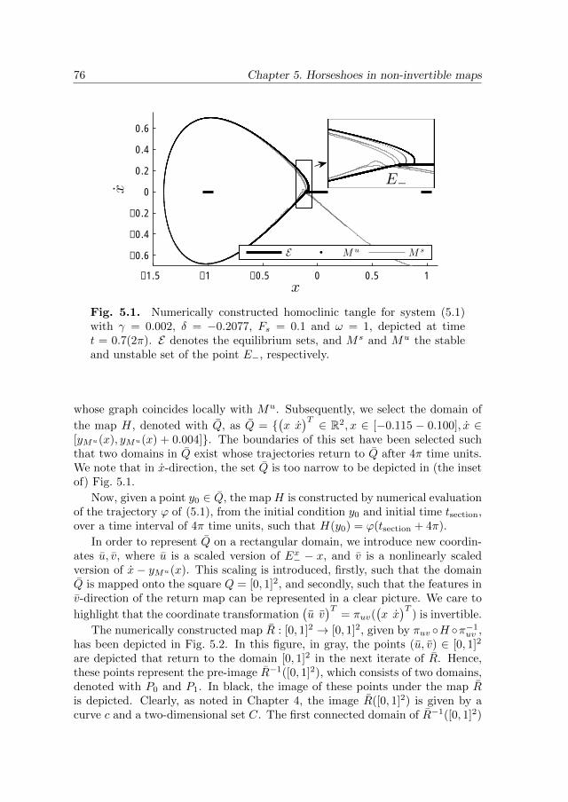
76 Chapter 5. Horseshoes in non-invertible maps
−1.5 −1 −0.5 0 0.5 1
−0.6
−0.4
−0.2
0
0.2
0.4
0.6
x
x
E M u M s
E−
Fig. 5.1. Numerically constructed homoclinic tangle for system (5.1)with γ = 0.002, δ = −0.2077, Fs = 0.1 and ω = 1, depicted at timet = 0.7(2π). E denotes the equilibrium sets, and Ms and Mu the stableand unstable set of the point E−, respectively.
whose graph coincides locally with Mu. Subsequently, we select the domain of
the map H, denoted with Q, as Q = (x x)T ∈ R2, x ∈ [−0.115 − 0.100], x ∈
[yMu(x), yMu(x) + 0.004]. The boundaries of this set have been selected suchthat two domains in Q exist whose trajectories return to Q after 4π time units.We note that in x-direction, the set Q is too narrow to be depicted in (the insetof) Fig. 5.1.
Now, given a point y0 ∈ Q, the map H is constructed by numerical evaluationof the trajectory ϕ of (5.1), from the initial condition y0 and initial time tsection,over a time interval of 4π time units, such that H(y0) = ϕ(tsection + 4π).
In order to represent Q on a rectangular domain, we introduce new coordin-ates u, v, where u is a scaled version of Ex− − x, and v is a nonlinearly scaledversion of x− yMu(x). This scaling is introduced, firstly, such that the domainQ is mapped onto the square Q = [0, 1]2, and secondly, such that the features inv-direction of the return map can be represented in a clear picture. We care to
highlight that the coordinate transformation(u v)T
= πuv((x x)T
) is invertible.
The numerically constructed map R : [0, 1]2 → [0, 1]2, given by πuv H π−1uv ,
has been depicted in Fig. 5.2. In this figure, in gray, the points (u, v) ∈ [0, 1]2
are depicted that return to the domain [0, 1]2 in the next iterate of R. Hence,these points represent the pre-image R−1([0, 1]2), which consists of two domains,denoted with P0 and P1. In black, the image of these points under the map Ris depicted. Clearly, as noted in Chapter 4, the image R([0, 1]2) is given by acurve c and a two-dimensional set C. The first connected domain of R−1([0, 1]2)

5.2 Discrete-time dynamical system 77
0 0.1 0.2 0.3 0.4 0.5 0.6 0.7 0.8 0.9 10
0.1
0.2
0.3
0.4
0.5
0.6
0.7
0.8
0.9
1
u
v
P0 P1
c
C
Fig. 5.2. Numerically constructed return map R for system (5.1) withγ = 0.002, δ = −0.2077, Fs = 0.1 and ω = 1. The gray domain denotesthe pre-image R−1([0, 1]2)∩[0, 1]2, the black domain the image R([0, 1]2)∩[0, 1]2
is crossed by the curve, but has an empty intersection with the strip.Motivated by these numerical results, in the following section, a class of
return maps is presented that has the same behaviour of the image and pre-image of the map R, as shown in Fig. 5.2. In fact, one may expect that thereexists a coordinate transformation such that the map R falls in the class of mapsintroduced in the next section.
5.2.2 Definition of the discrete-time system
In the remainder of this chapter, we consider the class of discrete-time dynamicalsystems given by a map R : [0, 1]2 → [0, 1]2 which can be described as:
R
((uv
))=
(
Ru(u)
Rvc(u, v)
), u ∈ p0 ∪ p1,
∅, otherwise,
(5.3a)
Rvc(u, v) =
fc(Ru(u)), u ∈ p0,
min(Rv(v), fc(Ru(u))), u ∈ p1,(5.3b)

78 Chapter 5. Horseshoes in non-invertible maps
Fig. 5.3. Pictorial illustration of the functions Ru, Rv and fc.
for(u v)T ∈ [0, 1]2. The sets p0 and p1 are closed intervals and are subsets
of (0, 12 ) and ( 1
2 , 1), respectively. In addition, the functions Ru, fc, and Rvsatisfy the properties formalised in the following assumption. These propertiesare pictorially illustrated in Fig. 5.3.
Assumption 5.1.
a. The continuous function Ru(u) maps both p0 and p1 onto [0, 1]. Further-more, there exist scalars λ, λ > 1 such that
λ|u0 − u1| ≤ |Ru(u0)−Ru(u1)| ≤ λ|u0 − u1| (5.4)
holds for any two points u0, u1 ∈ pi for i = 0 or i = 1.
b. The function fc is continuous and non-decreasing, fc(u+) = 0 for u+ ∈ p0,
and fc(u+) = 1
2 for u+ ∈ p1.
c. The function Rv is continuous, strictly monotonically decreasing, satisfies0 < Rv(v) < 1
2 for all v ∈ [0, 1], and there exists a λv ∈ (0, 1) such that
|Rv(v1)−Rv(v0)| < λv|v1 − v0|, ∀v0, v1 ∈ [0, 1]. (5.5)
Note that, if this assumption is satisfied, then the pre-image of the map R,as defined in (5.3), is given by two sets P0 = p0 × [0, 1] and P1 = p1 × [0, 1],similar to the numerical results shown in Fig. 5.2. In addition, similar to thecurve c and set C in this figure, the image of the map R consists of a curve(given by the graph of the function fc), and a two dimensional set, that is givenby the image of the map R from the points (u, v) ∈ [0, 1]2 for which u ∈ p1 andRv(v) < fc(Ru(u)).
In the following remark, a further motivation is presented for the study ofthe class of discrete-time systems given by (5.3) that satisfy Assumption 5.1.
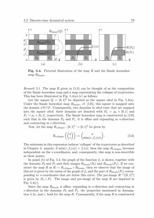
5.2 Discrete-time dynamical system 79
Fig. 5.4. Pictorial illustration of the map R and the Smale horseshoemap RSmale.
Remark 5.1. The map R given in (5.3) can be thought of as the compositionof the Smale horseshoe map and a map representing the collapse of trajectories.This has been illustrated in Fig. 5.4(a)-(c) as follows.
Let the square Q = [0, 1]2 be depicted as the square abcd in Fig. 5.4(a).Under the Smale horseshoe map RSmale, cf. [145], this square is mapped ontothe domain a′b′c′d′. Consequently, two domains in abcd exist that are mappedinto the square abcd; these domains are denoted with P0 = p0 × [0, 1] andP1 = p1 × [0, 1], respectively. The Smale horseshoe map is constructed in [145]such that in the domains P0 and P1, it is affine and expanding in u-directionand contracting in v-direction.
Now, let the map Rcollapse : [0, 1]2 → [0, 1]2 be given by
Rcollapse
((uv
)):=
(u
min(v, fc(u))
). (5.6)
The minimum in this expression induces ‘collapse’ of the trajectories as describedin Chapter 4: namely, if min(v, fc(u)) = fc(u), then the map Rcollapse becomesindependent on the v-coordinates, and, consequently, this map is non-invertibleat these points.
In panel (b) of Fig. 5.4, the graph of the function fc is shown, together withthe domains P0 and P1 and their images RSmale(P0) and RSmale(P1). If we con-struct the map R as R := Rcollapse RSmale, then we observe that the image ofthis set is given by the union of the graph of fc and the part of RSmale(P1) corres-ponding to v-coordinates that are below this curve. The pre-image R−1([0, 1]2)is given by P0 ∪ P1. The image and pre-image of the map R are depicted inFig. 5.4(c).
Since the map RSmale is affine, expanding in u-direction and contracting inv-direction in the domains P0 and P1, the properties mentioned in Assump-tion 5.1a. and c. hold for the map R. Consequently, if the map R is constructed

80 Chapter 5. Horseshoes in non-invertible maps
as R := Rcollapse RSmale, then Assumption 5.1 is automatically satisfied.We argue that this construction is a natural way to adapt the Smale horseshoe
map to capture the occurrence of the ‘collapse’ of trajectories. Together withthe simulation results presented in Section 5.2.1, this observation motivates thestudy of the iterates of the map R as presented in this chapter. C
Remark 5.2. When smooth differential equations are considered, a rigourous de-scription of the homoclinic tangle can be obtained using, for example, Melnikovfunctions [72] and the inclination, or lambda-lemma [127]. Together with a localdescription of the vector field near a hyperbolic equilibrium point, these res-ults allow to prove that a local domain Q exists for which trajectories returningto the same set are described by the Smale horseshoe map after an appropri-ate coordinate transformation, cf. [128]. In Appendix A.4, we will analyse thelocal dynamics near equilibrium sets that occur in the class of discontinuousdynamical systems considered in Chapter 4. We envision that a version of thelambda-lemma could be formulated that is applicable for this class of differentialinclusions. Indeed, further research is needed to formally attain such a result;once available, it would enable a rigourous description of the homoclinic tangleas sketched in Fig. 4.3. In that case, one may expect that the identification ofvertical and horizontal stripes, as formalised in [128], can be adapted to applyin our case. This would result in a rigourous proof that the map H as presentedin Chapter 4 and the map R described in Section 5.2.1 are contained, after acontinuous coordinate transformation, in the class of systems considered in thepresent chapter. C
5.2.3 Geometry of the limit set
In this section, we will describe the geometry of the invariant set of the map Rdefined in (5.3). For this purpose, firstly, we will study the forward iterates ofR, leading to a geometrical description of the set Mu :=
⋂∞i=0R
iQ, where weintroduced the set Q := [0, 1]2 for notational convenience. Subsequently, we will
employ an existing result that describes the setMs :=⋂0i=−∞RiQ, and describe
the intersection between both sets, leading to a description of the invariant setX of the map R.
The contraction in v-direction, as given in Assumption 5.1c., implies that theforward iterates of [0, 1] under the map Rv form two-dimensional sets that areincreasingly smaller in v-direction. From (5.3) we conclude that the set p0×[0, 1]is mapped onto a curve by the map R. These observations are instrumental in theproof of the following lemma, that states that the setMu :=
⋂∞i=0R
iQ consistsof a set of curves hi, i ∈ N, that accumulates to a curve h?, and, consequently,the setMu does not have a fractal structure. In addition, this lemma introducesa labeling of the curves hi, i ∈ N, inMu which facilitates the analysis of the mapR. This labelling is illustrated in Fig. 5.5. In the formulation of this lemma, weuse the sets P0 := p0 × [0, 1] and P1 := p1 × [0, 1].

5.2 Discrete-time dynamical system 81
Fig. 5.5. Pictorial illustration of the setMu where the curve h? and thelabelling of the curves hi, i ∈ N, is shown.
Lemma 5.1. Consider the map R given in (5.3) and let Assumption 5.1 besatisfied. The set Mu can be described by
Mu = h? ∪∞⋃i=0
hi (5.7)
where each hi, i ∈ N∪?, denotes a curve in Q that can be described as the graphof a continuous function hi(u), that is defined for u ∈ [0, 1] and constant foru ∈ p0 and u ∈ p1. The curves hi, i ∈ N∪?, are such that hi∩hj ∩P1 = ∅ andhi∩P0 = hj ∩P0 for all i 6= j, i, j ∈ N∪?. In addition, the curves hi convergeto the curve h? for i → ∞. Finally, the map R is such that hi+1 = R(hi ∩ P1)for i ∈ N.
Proof. The proof of this lemma is given in Appendix A.3.
The backward iterates of the map R behave similar to the backward dynamicsof the Smale horseshoe map. Hence, we will only briefly describe the geometryof the set Ms =
⋂0i=−∞RiQ.
Observe that given Assumption 5.1, equation (5.3) implies that R((u, v)T
) ∈Q if Ru(u) ∈ [0, 1], and, in addition, that the dynamics in u-direction is notdepending on the v-coordinate. By Assumption 5.1c., the mapR is contracting in
v-direction, such that we conclude that⋂0i=−lR
iQ is equal to
(0⋂
i=−lRiu([0, 1])
)×
[0, 1] for all l ≥ 1. Hence, we may restrict our attention to the interval mapRu : [0, 1]→ [0, 1].
If Assumption 5.1 is satisfied, then, using the approach of [90], one can show
that⋂0i=−∞Riu([0, 1]) is a Cantor set. Consequently, the setMs =
⋂0i=−lR
iQ =(⋂0i=−∞Riu([0, 1])
)× [0, 1] is described geometrically by the Cartesian product
of a Cantor set and the interval [0, 1].
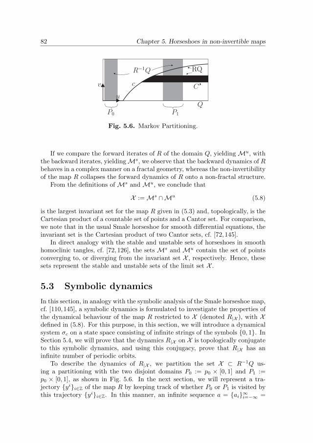
82 Chapter 5. Horseshoes in non-invertible maps
Fig. 5.6. Markov Partitioning.
If we compare the forward iterates of R of the domain Q, yieldingMu, withthe backward iterates, yieldingMs, we observe that the backward dynamics of Rbehaves in a complex manner on a fractal geometry, whereas the non-invertibilityof the map R collapses the forward dynamics of R onto a non-fractal structure.
From the definitions of Ms and Mu, we conclude that
X :=Ms ∩Mu (5.8)
is the largest invariant set for the map R given in (5.3) and, topologically, is theCartesian product of a countable set of points and a Cantor set. For comparison,we note that in the usual Smale horseshoe for smooth differential equations, theinvariant set is the Cartesian product of two Cantor sets, cf. [72, 145].
In direct analogy with the stable and unstable sets of horseshoes in smoothhomoclinic tangles, cf. [72, 126], the sets Ms and Mu contain the set of pointsconverging to, or diverging from the invariant set X , respectively. Hence, thesesets represent the stable and unstable sets of the limit set X .
5.3 Symbolic dynamics
In this section, in analogy with the symbolic analysis of the Smale horseshoe map,cf. [110,145], a symbolic dynamics is formulated to investigate the properties ofthe dynamical behaviour of the map R restricted to X (denoted R|X ), with Xdefined in (5.8). For this purpose, in this section, we will introduce a dynamicalsystem σc on a state space consisting of infinite strings of the symbols 0, 1. InSection 5.4, we will prove that the dynamics R|X on X is topologically conjugateto this symbolic dynamics, and using this conjugacy, prove that R|X has aninfinite number of periodic orbits.
To describe the dynamics of R|X , we partition the set X ⊂ R−1Q us-ing a partitioning with the two disjoint domains P0 := p0 × [0, 1] and P1 :=p0 × [0, 1], as shown in Fig. 5.6. In the next section, we will represent a tra-jectory yii∈Z of the map R by keeping track of whether P0 or P1 is visited bythis trajectory yii∈Z. In this manner, an infinite sequence a = ai∞i=−∞ =
5.3 Symbolic dynamics 83
(. . . a−1.a0a1 . . .) ∈ 0, 1Z is obtained, where ai ∈ 0, 1 for all i. In The-orem 5.2, which we will present in the next section, we show that each traject-ory of R can be represented in such strings of symbols. This relation betweentrajectories of the map R and strings of symbols a ∈ 0, 1Z motivates the re-mainder of the present section, where we will formally introduce a dynamicalsystem on the state space 0, 1Z. Using the nomenclature of [158], we call everya ∈ 0, 1Z a point, and if we represent a point a ∈ 0, 1Z as (. . . a−1.a0a1 . . .),then the dot is followed by the symbol a0 with index 0.
In [110, 145], the dynamics of the Smale horseshoe map, which is an in-vertible map, is shown to be topologically conjugate to an invertible dynamicalsystem defined on 0, 1Z, namely, the full 2-shift, which can be described by the
edge shift on a graph with transition matrix A =
(1 11 1
)as formalised in [110].
In [52, 83], a cusp horseshoe map is considered, that is motivated by the singu-lar perturbation of a smooth dynamical system. It is shown that this map isnon-invertible at one particular point in state space, coinciding with the cuspposition. In [52], a topological conjugacy is constructed between the cusp horse-shoe map and a shift map defined on a quotient space of symbols. The maindifference between the map R and the cusp horseshoe maps considered in [52,83]is that the map R considered in the present chapter is non-invertible at morethan one point.
In fact, in our case, the return map R is not invertible for all points mappedinto the set P0. Hence, for points y0 ∈ P0 ∩ X , the pre-image R−1(y0) is set-valued, although R−1(y1) is a singleton for y1 ∈ P1 ∩ X .
Since R is not invertible at all points, we will define a symbolic dynamics on aquotient space of 0, 1Z, which is defined with the following equivalence. Essen-tially, this equivalence implies that two points a, b ∈ 0, 1Z are equivalent whentheir current and future symbols ai, i ∈ [0,∞), coincide, and their past symbolsai, i ∈ (−∞,−1], coincide for i ≥ −k, where k ≥ 0 denotes the minimum indexsuch that a−k = 0. If a shift map ai → ai+1, i ∈ Z, defines the discrete-timesystem on this state space, then the trajectories with distinct ‘histories’ collapseonto each other when a0 = 0, whereas no collapse occurs when a0 = 1.
Definition 5.1. Points a, b ∈ 0, 1Z are equivalent, denoted a ∼ b, when a = bor when there exists an integer k ≥ 0 such that
ai = bi, ∀i ∈ [1,∞), (5.9)
ai = bi = 1, ∀i ∈ [−k + 1, 0], (5.10)
a−k = b−k = 0, (5.11)
holds.
This is indeed an equivalence relation, since a ∼ a,∀a ∈ 0, 1Z, the relationis symmetric as (5.9)-(5.11) are symmetric for each index i ∈ Z, and a ∼ b and
84 Chapter 5. Horseshoes in non-invertible maps
b ∼ c imply a ∼ c. Hence, we can formulate the quotient space, cf. [93]:
Sc := 0, 1Z/ ∼, (5.12)
which implies that two points a1, a2 ∈ 0, 1Z are identified with each otherwhen a1 ∼ a2. On the space Sc, we define the metric ρc as follows, where weadopt the convention 2−∞ = 0.
Definition 5.2. Given two points a, b ∈ Sc, let k be a nonnegative integer or∞, such that ai = 1 for all i ∈ [−k+ 1, 0] and a−k = 0 if k is finite. If ` denotesthe maximal integer or ∞ such that ai = bi for all i ∈ [max(−k,−`), `], then wedefine:
ρc(a, b) = 2−`. (5.13)
Remark 5.3. Observe that ρc(a, b) = infc∈0,1Z,c∼b
ρ(a, c), with ρ(a, c) = 2−m, and
m the maximal integer such that ai = ci for i ∈ [−m,m]. The metric ρ(a, c), fora, c ∈ 0, 1Z is the metric presented in [110]. C
We observe that ρc is a metric on Sc, as it satisfies the symmetry requirementρc(a, b) = ρc(b, a), triangle inequality ρc(a, c) ≤ ρc(a, b) + ρc(b, c) and, finally,ρc(a, b) = 0 if and only if a ∼ b.
We define the forward dynamics on Sc as a shift σc : Sc → Sc on the symbolsas follows:
σc((. . . a−1.a0a1a2 . . .)) = (. . . a−1a0.a1a2 . . .), (5.14)
such that (σc(a))i = ai+1, ∀i ∈ Z.We note that the shift map σc : Sc → Sc is a continuous map which is not
invertible. The pre-image of σc is given by:
σ−1c ((. . . a−2a−1.a0a1 . . .)) ∈
(. . . a−2.a−1a0a1a2 . . .), a0 = 1,b ∈ Sc, σc(b) ∼ a, a0 = 0.
(5.15)
The pre-image σ−1c is set-valued for certain points in Sc, which enables a
comparison between the map σc on Sc and the map R|X defined on X , whichalso is non-invertible at the points x where R(x) ∈ P0. Therefore, both thedynamical systems (X , R|X ) and (Sc, σc) are continuous and, for part of theirdomain of definition, the maps R|X and σc are not invertible. In the next section,the collapse of trajectories in the map R|X will be related to iterations of theshift map σc such that the symbol (σc(a))0 becomes 0.
5.4 Topological conjugacy between symbolic dy-namics and discrete-time system
In this section, the symbolic dynamics presented in the previous section is shownto be topologically conjugate to the return map R|X , where we adopt the defini-tion of topological conjugacy from [142, Definition 8.1], which is given as follows.
5.4 Topological conjugacy 85
Definition 5.3. Let M and N be two topological spaces and Φ : M → M andΨ : N → N two continuous maps. A homeomorphism τ : M → N is a topologicalconjugacy if τ Φ = Ψ τ , that is, if the following diagram commutes:
MΦ //
τ
M
τ
N
Ψ// N
Two dynamical systems (M,Φ) and (N,Ψ) are topologically conjugate if there isa topological conjugacy between them.
We can now present the main theorem of this chapter. This theorem statesthat (Sc, σc) is topologically conjugate to (X , R|X ) and, in addition, presents amapping τ that is a topological conjugacy between both systems.
Theorem 5.2. Consider the map R|X : X → X , which is defined as the re-striction of the map R given in (5.3) to the invariant set X as in (5.8), and letthe map σc : Sc → Sc be given in (5.14). In addition, let Assumption 5.1 besatisfied. Consider hi, i ∈ N as defined in Lemma 5.1 and let the function κ(y),for y ∈ X , denote the minimum integer such that y ∈ hκ(y), or κ(y) = ∞ ify 6∈ hi for all i ∈ N. Let τ : X → Sc be given by:
(τ(y))i =
0, i ∈ (−∞,−κ(y)− 1],
1, i ∈ [−κ(y),−1],
0, i ∈ [0,∞) ∧Ri(y) ∈ P0,
1, i ∈ [0,∞) ∧Ri(y) ∈ P1.
(5.16)
The function τ is a topological conjugacy, such that (Sc, σc) is topologically con-jugate to (X , R|X ).
Proof. The proof of this theorem is given in Appendix A.3.
Analogously to the standard argument for the full two-shift on 0, 1Z, asanalysed e.g. in [145], we observe that the dynamical system (Sc, σc) containsan infinite number of periodic orbits. Initial conditions of such periodic orbitsare given by (0)′, (1)′, (01)′, (001)′, (011)′, . . ., where (z)′ denotes an infiniterepetition of the block z. The period of these orbits is equal to the length of theblock z. Since the topological conjugacy τ given in Theorem 5.2 connects eachof these periodic orbits of (Sc, σc) to a periodic orbit of (X , R|X ), we directlyobtain the following corollary.
Corollary 5.3. The dynamical system (X , R|X ) contains an infinite number ofperiodic orbits.

86 Chapter 5. Horseshoes in non-invertible maps
We will now show that the dynamical system (X , R|X ) is topologically trans-itive. To define this property, we call an orbit yii∈Z dense in a set Q if it isarbitrarily close to any point p ∈ Q.
Definition 5.4 ( [90]). A dynamical system (X , R|X ) is topologically transitiveif there exists a point q ∈ X such that its orbit Ri|X (q)i∈N is dense in X.
Lemma 5.4. The dynamical system (X , R|X ) is topologically transitive.
Proof. The proof of this lemma is given in Appendix A.3.
Corollary 5.3 and Lemma 5.4 imply that the dynamical system (X , R|X )has an infinite number of periodic orbits, and that the system is topologicallytransitive. Both of these properties are known to hold as well for the Smalehorseshoe map, cf. [145]. For this reason, we argue that the map R is closelyrelated to the Smale horseshoe map. The geometry of the limit set X , however,is essentially different from the smooth horseshoe, as discussed in Section 5.2.3.In addition, in contrast to the smooth horseshoe dynamics, the trajectories inX cannot be uniquely continued in the backward direction of time.
5.5 Conclusion
In this chapter, a class of discrete-time systems is studied that consists of non-invertible maps that are closely related to the Smale horseshoe map. We expectthat this class of maps describes the trajectories of mechanical systems with dryfriction and periodic perturbation given in Chapter 4. The discrete-time systemsconsidered here are given by maps that are continuous, but not invertible. Wehave described the geometry of the limit sets of these maps, have shown thatthe limit set is transitive, and have proven that an infinite number of periodicorbits exist.
The analysis of the trajectories in the limit set was performed by formulatinga new type of symbolic dynamics, where a symbolic state space is designed witha quotient structure. Due to this structure, a shift map on this state space canrepresent the non-invertibility of the horseshoe-like map. We have proven thatthis symbolic dynamics is topologically conjugate to the horseshoe-like map. Inthis manner, we have identified a dense orbit in the limit set of this map, andhave proven that the map has an infinite number of periodic orbits. Due tothese similarities with the limit set of the Smale horseshoe map, we refer tothis limit set as a horseshoe. However, in comparison with the limit set of theSmale horseshoe map, the geometry of this limit set is qualitatively different,and trajectories in the horseshoe can not be continued uniquely in the reverseddirection of time.

Part II
Tracking control for hybridsystems

Chapter 6
Tracking control for hybridsystems with state-triggered
jumps
Abstract – This chapter addresses the tracking problem in which the controller should
stabilise time-varying reference trajectories of hybrid systems. Despite the fact that discrete
events (or jumps) in hybrid systems can often not be controlled directly, as, e.g., is the case
in impacting mechanical systems, the controller should still stabilise the desired trajectory. A
major complication in the analysis of this hybrid tracking problem is that, in general, the jump
times of the plant do not coincide with those of the reference trajectory. Consequently, the
conventional Euclidean tracking error does not converge to zero, even if trajectories converge
to the reference trajectory in between jumps, and the jump times converge to those of the
reference trajectory. Hence, standard control approaches can not be applied. We propose a
novel definition of the tracking error that overcomes this problem and formulate Lyapunov-
based conditions for the global asymptotic stability of the hybrid reference trajectory. Using
these conditions, we design hysteresis-based controllers that solve the hybrid tracking problem
for two exemplary systems, including the well-known bouncing ball problem.
6.1 Introduction
Hybrid systems, such as for example robotic systems with impacts, digitally con-trolled physical systems, electrical circuits with switches, and models of chemicalreactors with valves, can be characterised by the interaction between continuous-time dynamics and discrete events, cf. [67, 111, 139]. Due to this interaction,hybrid systems can show more complex behaviour than can occur in ordinary
This chapter is based on [21], and parts have appeared in [20].

90 Chapter 6. Tracking control for hybrid systems with state-triggered jumps
differential equations (ODEs) or discrete-time systems. Consequently, conven-tional control approaches are often not directly applicable.
Most existing results in the literature on hybrid control systems deal withthe stability of time-independent sets (especially with equilibrium points), suchthat the stability can be analysed using Lyapunov functions, see, e.g., [40,67,76,104,109,112,117,139,141]. Essentially, such a set is asymptotically stable when aLyapunov function decreases both during flow and jumps (i.e., discrete events),see, e.g., [40, 67, 117]. Extensions of these results allow for Lyapunov functionsthat increase during jumps, as long as this increase is compensated for by alarger decrease during flow, or vice versa. Such results are reviewed in [81,141].Using these Lyapunov-based stability results, several control strategies have beendeveloped to stabilise time-independent sets for hybrid systems, see, e.g., [67,76].
Few results exist where controllers are designed to make a system track agiven, time-varying, reference trajectory, that exhibits both continuous-time be-haviour and jumps. In this chapter, we consider reference trajectories that aresolutions of the plant for a given, time-dependent reference input. When thejump times of the plant trajectories can be guaranteed to coincide with jumpsof the reference trajectory, then stable behaviour of the Euclidean tracking erroris possible and several tracking problems have been solved in this setting, see,e.g., [35, 106, 134, 135, 137, 160, 161]. In [75], observer problems are consideredfor a class of hybrid systems where a similar condition is exploited, namely, thatthe jumps of the plant and the observer coincide. When jump times of the planttrajectory x and reference trajectory r can be ensured to coincide, standardLyapunov tools are applicable to study the evolution of x− r along trajectories.However, requiring the jump times of plant and reference trajectories (or plantand observer) to coincide is a strong condition that limits the applicability ofthese results. For example, this can not be ensured for general hybrid systemswith state-triggered jumps, such as models of mechanical systems with unilateralconstraints, cf. [66, 104].
In hybrid systems with state-triggered jumps, the jump times of the plantand the reference trajectory are in general not coinciding. To illustrate thisbehaviour, we consider the trajectories of a scalar hybrid system with statex ∈ [0, 1], where the continuous-time evolution is given by
x = 1 + u(t), x ∈ [0, 1], (6.1a)
where u is a bounded control input and jumps occur according to:
x+ = 0, x = 1. (6.1b)
Now, consider the signal r = t mod 1 as a reference trajectory, where mod de-notes the modulus operator, and observe that r is the solution of (6.1) from theinitial condition r0 = 0 with u(t) ≡ 0. Suppose that a control signal u is con-structed such that a plant trajectory x tracks the reference trajectory r (in fact,

6.1 Introduction 91
0 1 2 3 4 5 6 7 8
0
0.5
1
0 1 2 3 4 5 6 7 8
−0.5
0
0.5
1
Fig. 6.1. (a) Exemplary trajectories of (6.1). (b) Euclidean trackingerror |r − x|.
such a controller will be designed in Section 6.5.1), then we expect behaviour asgiven in Fig. 6.1, where the state x and reference trajectory r converge to eachother away from the jump times, and the jump times show a vanishing mismatch.During the time interval caused by this jump-time mismatch, the Euclidean er-ror |x − r| is large, as shown in Fig. 6.1(b). Since this behaviour also occursfor arbitrarily small initial errors |x − r|, the Euclidean error displays unstablebehaviour in the sense of Lyapunov. This “peaking behaviour” was observedin [35,75,104,116,134,135], and is expected to occur in all hybrid systems withstate-triggered jumps when considering tracking or observer design problems.However, although the Euclidean error may display undesirable properties, froma control engineering point of view, the trajectories shown in Fig. 6.1 are con-sidered to exhibit desirable behaviour. Therefore, it seems that the evaluation ofthe tracking error using non-Euclidean distance functions might be advantage-ous for a class of hybrid systems, such as the example in (6.1). For this reason,we formulate a different notion of tracking in this chapter, that considers thebehaviour shown in Fig. 6.1 as a proper solution, since the jump times of theplant converge to the jump times of the reference and the distance between theplant and reference trajectories converges to zero during time intervals withoutjumps. This tracking notion is less restrictive than notions requiring stabilityof the Euclidean error (cf. [35, 106, 134, 135, 137]), such that the class of hybridsystems that can be considered is widened significantly.
Several approaches have already been presented in the literature to formalisetracking notions where controllers that solve the resulting tracking problem areallowed to induce behaviour as shown in Fig. 6.1. However, in these approachesit is not clear how to formulate conditions under which such tracking problemsare solved. In [63, 116], the tracking of a billiard system is considered using theconcept of “weak stability”, which implies that the position of the ball is alwaysrequired to be close to the reference trajectory, but the error in velocity is notstudied for a small time interval near the jump instances. In addition, the con-vergence of jump times is required. In [62], this approach is extended to a largerclass of hybrid systems. However, since no requirements are imposed close to the

92 Chapter 6. Tracking control for hybrid systems with state-triggered jumps
jump times, such a tracking problem definition needs knowledge of complete tra-jectories. Alternatively, the notion of weak stability is employed in [36, 121] forunilaterally constrained mechanical systems with reference trajectories where allimpacts, if they occur, show accumulation points (i.e., Zeno behaviour), followedby a time interval where the constraint is active. In the very recent conferencepapers [59,60], tracking control problems for billiard systems are formulated byrequiring asymptotic stability of a set of trajectories, consisting of the refer-ence trajectory and its mirror images, when reflected in the boundaries of thebilliard. This independent research effort resulted in a related control problemformulation and controller design approach as those given for the bouncing ballexample in Section 6.5.2 of this thesis. In this chapter, we aim to present ageneral framework for addressing tracking problems for a relatively generic classof hybrid systems (not focussing on a class of mechanical systems with unilat-eral constraints as in [59, 60]). Alternatively, in [116], it is suggested to employthe stability concept of Zhukovsky (see [108]). Using this stability concept, theplant trajectory is compared with the reference trajectory after a rescaling oftime for the plant trajectory, i.e., the error x(ρ(t))− r(t) should behave asymp-totically stable, where a function ρ(t) is used with limt→∞(ρ(t) − t) = 0. As asecond alternative, a Hausdorff-type metric between the graphs of the referenceand plant trajectory is suggested in [118]. Both the rescaling function ρ forZhukovsky stability and the Hausdorff-type metric require complete knowledgeof the trajectories, and, consequently, it is not clear how these concepts can beused to solve the design problem of tracking controllers.
In order to study tracking problems with non-matching jump times, we pro-pose an alternative approach using a non-Euclidean distance between the plantand reference states, where convergence of this distance measure corresponds tothe desired notion of tracking. Since this distance measure incorporates informa-tion on the “closeness” of the reference state and plant state at each time instant,the tracking problem can be formulated based on the time evolution of the dis-tance measure evaluated along trajectories of the closed-loop system. This factis instrumental in our approach, as it allows us to derive sufficient conditionsunder which the tracking problem is solved, that are formulated using the in-stantaneous state, its time-derivatives, and the jumps that can occur. Since suchinformation is encoded directly in the hybrid system description, this propertyis an advantage of our approach when compared to the analysis of [62, 63, 116],where convergence of jump times is proven using complete trajectories. In ad-dition to this new formulation of the tracking problem for hybrid systems, wepresent sufficient conditions that guarantee that this problem is solved. In thismanner, we will provide a general framework for the formulation and analysis oftracking problems for hybrid systems. Although we do not address the synthesisproblems of tracking controllers in its full generality, we are convinced that theresults of this chapter provide an indispensable stepping stone towards such asynthesis procedure. In fact, the applicability of the presented framework for the
6.2 Modelling of hybrid control systems 93
design of tracking controllers will be demonstrated for two exemplary systems,including a mechanical system with a unilateral constraint.
The main contributions of this chapter can be summarised as follows. First,the proposed reformulation of the tracking notion using a non-Euclidean track-ing error measure allows to state and analyse tracking problems for a large classof hybrid systems, and these tracking problems are not rendered infeasible bythe “peaking” of the Euclidean tracking error. Second, existing Lyapunov-typestability conditions, both with and without an additional average dwell-timecondition, are extended to allow non-Euclidean distance functions, yielding suf-ficient conditions for the global asymptotic stability of time-invariant sets. Thisresult allows to formulate conditions that ensure that the new tracking problemis solved. Third, in two examples we show that the new tracking error measurecan be used to design controllers that solve the tracking problem.
This chapter is organised as follows. In Section 6.2, the hybrid system modeland the corresponding solution concept are introduced. Subsequently, in Sec-tion 6.3, requirements are formulated for the design of appropriate trackingerror measures, and the tracking problem is formulated. Section 6.4 containsLyapunov-type conditions that are sufficient for the tracking problem to besolved. The results of this chapter are illustrated with examples on control-ler synthesis for the hybrid tracking problem in Section 6.5, and conclusions areformulated in Section 6.6.
Notation: Rn denotes the n-dimensional Euclidean space; R the set of realnumbers; R≥0 the set of nonnegative real numbers; N the set of natural numbersincluding 0. Let Int(S) denote the interior of a set S ⊂ Rn, ∂S the boundaryof the set, cl(S) its closure, co(S) the smallest closed convex hull containing S,and µ(S) denotes its Lebesgue measure. Let f : Rm ⇒ Rn denote a set-valuedmapping from Rm to subsets of Rn. Given vectors x ∈ Rn and y ∈ Rm, |x|denotes the Euclidean vector norm, col(x, y) denotes (xT yT )T and ∇x denotes∂∂x . A function α : [0,∞)→ [0,∞) is said to belong to class-K∞ (α ∈ K∞) if itis continuous, zero at zero, strictly increasing and unbounded. Given a Lipschitzfunction V : Rm → R, ∂CV denotes the generalized differential of Clarke, i.e.,∂CV = co(lim∇xV (xi)| xi → x, xi 6∈ ΩV ), where ΩV denotes the set of measurezero where ∇xV is not defined.
6.2 Modelling of hybrid control systems
In this chapter, we employ the framework of hybrid inclusions described in [67],allowing the continuous-time dynamics (flow) to be time-dependent, such thatthe hybrid system is given by
x ∈ F (t, x, u), x ∈ C ⊆ Rn, (6.2a)
x+ ∈ G(x), x ∈ D ⊆ Rn, (6.2b)
94 Chapter 6. Tracking control for hybrid systems with state-triggered jumps
with F : R≥0 × C × U ⇒ Rn, G : D ⇒ Rn, where x ∈ F (t, x, u) describes thecontinuous-time (flow) dynamics that is feasible when states x are in the flowset C ⊆ Rn, and jumps can occur according to x+ ∈ G(x) when states are in thejump set D ⊆ Rn. The control inputs u ∈ U ⊂ Rm are assumed to be containedin the compact set U . Moreover, only trajectories from initial conditions in C∪Dare considered. Note that the reset map G in (6.2b) is not dependent on time orthe actuator inputs u, and models purely state-triggered jumps. We adopt theconvention that G(x) = ∅ when x 6∈ D.
The following technical assumption is imposed on the data of the hybridsystem (6.2).
Assumption 6.1. For any bounded set C1 ⊂ cl(C), the set F (t, x, u) is non-empty, measurable and essentially bounded for all (t, x, u) ∈ R≥0 × C1 × U andG(x) ⊂ C ∪D is non-empty and bounded for all x ∈ D.
In order to define solutions of the hybrid system (6.2), we assume that the in-put u satisfies u ∈ U(t, x) ⊆ U , which allows, firstly, to evaluate solutions of thehybrid systems when the input is a time signal U(t, x) = U(t), and secondly, toconsider discontinuous, state-dependent control laws, e.g., sliding mode control-lers. We consider solutions ϕ of the hybrid system (6.2) in the sense of [67], suchthat ϕ is defined on a hybrid time domain domϕ ⊂ [0,∞)×N as follows. A hy-brid time instant is given as (t, j) ∈ domϕ, where t denotes the continuous timelapsed, and j denotes the number of experienced jumps. The arc ϕ is a solutionof (6.2) associated to u when jumps satisfy (6.2b) and ϕ is a Filippov solutionof (6.2a) during flow, cf. [58]. This implies ϕ(t, j+ 1) ∈ G(ϕ(t, j)) for all (t, j) ∈domϕ such that (t, j + 1) ∈ domϕ and1 d
dtϕ(t, j) ∈ F (t, ϕ(t, j), U(t, ϕ(t, j))) foralmost all t ∈ Ij := t| (t, j) ∈ domϕ and all j such that Ij has non-empty in-terior, where F (t, x, U(t, x)) =
⋂δ≥0
⋂µ(N)=0 coF (t, x, U(t, x)), |x− x| ≤ δ, x 6∈
N represents the convexification of the vector field as defined by Filippov, wheresets N of Lebesgue measure zero are excluded. The solution ϕ is said to be com-plete if domϕ is unbounded, which, for example, holds for all trajectories of(6.2) if C ∪D is invariant under the dynamics of (6.2). The hybrid time domaindomϕ is called unbounded in t-direction when for each T ≥ 0 there exist a jsuch that (T, j) ∈ domϕ. In this chapter, we only consider maximal solutions,i.e., solutions ϕ for which the domain domϕ can not be extended.
Analogous to the common approach in tracking control for ODEs, we considerreference trajectories r that are unique solutions to (6.2), i.e., solutions to r ∈F (t, r, uref(t)), r ∈ C, r+ ∈ G(r), r ∈ D, for a given input signal u = uref(t) ∈ Uand initial condition r0. We design a control law for u to obtain asymptotictracking, in an appropriate sense, of the reference trajectory r by the resultingclosed-loop plant. We consider feedback controllers that are static, where u =
1We employ, with a slight abuse of notation, the convention that F (t, ϕ(t, j), U) denotesf ∈ Rn|f = F (t, ϕ(t, j), u), u ∈ U.
6.2 Modelling of hybrid control systems 95
uc(t, r, x) ∈ U , or dynamic, where the (possibly hybrid) controller has an internalstate η ∈ Rp and is described by
η ∈ Fc(t, r, x, η), (r, x, η) ∈ Cc,η+ ∈ Gc(r, x, η), (r, x, η) ∈ Dc,u = uc(t, r, x, η),
(6.3)
and assume that this controller satisfies Assumption 6.1. In order to study thestability of the closed-loop system, we create an extended hybrid system withstate q = col(r, x, η). The dynamics of this extended hybrid system is given by
q ∈ Fe(t, q), q ∈ Ce := (C2 × Rp) ∩ Cc, (6.4a)
q+ ∈ Ge(q) =
col(G(r), x, η), q ∈ (D × (C ∪D)× Rp) ∩ (Cc ∪Dc)col(r,G(x), η), q ∈ ((C ∪D)×D × Rp) ∩ (Cc ∪Dc)col(r, x,Gc(r, x, η)), q ∈ Dc,
(6.4b)
where Fe(t, q) := col(F (t, r, uref(t)), F (t, x, uc(t, r, x, η)), Fc(t, r, x, η)), and wedenote the domain of Ge in (6.4b) with De. We refer to Fe, Ge, Ce and De asthe data of system (6.4).
The main advantage of considering this extended hybrid system (6.4) is thata joint hybrid time domain is created, where hybrid times (t, j) ∈ dom q denotethe continuous time t lapsed, and j gives the total number of jumps that occurredin x, r and η. Hence, one can compare the reference state r with the plant state xfor each time instant (t, j) ∈ dom q. Let Ii,i denote the unit matrix of dimensioni× i, and let Oi,j be a zero matrix of dimension i× j. Defining
r(t, j) := (In,n On,n On,p) q(t, j)x(t, j) := (On,n In,n On,p) q(t, j)η(t, j) := (Op,n Op,n Ip,p) q(t, j),
(6.5)
allows to introduce a tracking error d(r, x) and formulate a tracking problem byrequiring, firstly, that d(r(t, j), x(t, j)) remains small provided that the initialerror d(r(0, 0), x(0, 0)) is small, and secondly, that d(r(t, j), x(t, j)) converges tozero for t+j →∞, (t, j) ∈ dom q, provided that this limit exists. In fact, we willformulate the tracking problem by requiring asymptotically stable behaviour ofd(r(t, j), x(t, j)), and, in two exemplary systems, we will design controllers thatguarantee that the domain dom q is unbounded in t-direction, such that the limitt→∞ exists and, for example, no accumulation of jump times (known as Zenobehaviour, cf. [67]) will occur.
Remark 6.1. If two distinct trajectories x and r from (6.2) are considered, then,in general, dom r 6= domx. In this case, if one would define a time-dependenttracking error at time (t, j) ∈ domx, then it would not be not clear what time(tr, jr) ∈ dom r is appropriate to use in a comparison of x and r. Such problems
96 Chapter 6. Tracking control for hybrid systems with state-triggered jumps
are avoided by studying the extended dynamics in (6.4), where the functions x :dom q → C ∪D, r : dom q → C ∪D and η : dom q → Rp are reparameterisationsof the functions x : domx → C ∪ D, r : dom r → C ∪ D and η : dom η → Rp,respectively. C
6.3 Formulation of the tracking control problem
In Section 6.3.1, we introduce distance functions d(r, x) suitable to compare theplant trajectory with the reference trajectory, such that asymptotically stablebehaviour of d(r(t, j), x(t, j)) corresponds to appropriate tracking. Subsequently,in Section 6.3.2 we introduce asymptotic stability with respect to the trackingerror d(r, x), and formalise the hybrid tracking problem.
6.3.1 Definition of the tracking error measure
In hybrid systems where jumps of the plant are state-triggered, as in (6.2),asymptotically stable behaviour of the Euclidean error |x − r| is generally im-possible to achieve due to the peaking phenomenon, see Fig. 6.1, which, evenwhen x and r converge to each other away from the jump instances, occurs whenjump times of the reference and plant trajectories show a small, possibly asymp-totically vanishing, mismatch. To illustrate this in the exemplary system (6.1),observe that if |x − r| converges to zero during continuous-time evolution andjumps are not exactly coinciding, then, by the structure of the jump map (6.1b),|x−r| ≈ 1 directly after a jump of either x or r. Since this peaking phenomenonrenders all tracking problems infeasible that require stable behaviour of the Eu-clidean error |x − r|, in this chapter, we present a novel approach to comparetrajectories of the plant with a reference trajectory. For hybrid systems withstate-triggered jumps given in (6.2), we will show that the exact properties ofthe jumps can be used to compare a reference trajectory with a plant trajectory,when one of them just experienced a jump, and the other did not. A distancefunction between two trajectories that enables such a comparison incorporatesthe structure of the jumps, as described in (6.2b), and hence is tailored to thespecific hybrid system. In this chapter, we employ distance functions, denotedas d(r, x), to formulate and solve the tracking problem.
We consider distance functions d(r, x) that are not sensitive to jumps of theplant and the reference trajectory, i.e. d(r, x) = d(gr, x) for r ∈ D, gr ∈ G(r)and d(r, x) = d(r, gx) for x ∈ D, gx ∈ G(x). In this manner, stability withrespect to the distance function d(r, x) is not influenced by the jumps of theplant or the reference trajectory. As we will show below, a distance functiond(r, x) is an appropriate measure to compare a reference trajectory r with a planttrajectory x when it satisfies the following conditions. We adopt the notationG0(x) = x, ∀x ∈ C ∪D and Gk+1(x) = G(Gk(x)), k = 0, 1, 2, . . .. Recall thatG(x) = ∅ when x 6∈ D.
6.3 Formulation of the tracking control problem 97
Definition 6.1. Consider a hybrid system H given by (6.2) that satisfies As-sumption 6.1. A non-negative function d : cl((C∪D)× (C∪D))→ R≥0 is calleda distance function compatible with H when it is continuous and satisfies
d(r, x)=0⇔(∃k1, k2 ∈ N, such that Gk1(x) ∩Gk2(r) 6= ∅),∀(r, x) ∈ cl(C ∪D)2,(6.6a)
x ∈ C ∪D| d(r, x) < β is bounded, ∀r ∈ C ∪D,β ≥ 0, (6.6b)
d(r, x) = d(r, gx), ∀x ∈ D, gx ∈ G(x), r ∈ C ∪D, (6.6c)
d(r, x) = d(gr, x), ∀r ∈ D, gr ∈ G(r), x ∈ C ∪D. (6.6d)
In this chapter, we will study stability of the set where d(r, x) is zero forsystem (6.4). Using (6.6a), in this set, (∃k1, k2 ∈ N, such that Gk1(x)∩Gk2(r) 6=∅) holds true, such that the distance d(r, x) is zero if and only if either r = x (suchthat the right-hand side of the implication in (6.6a) holds with k1 = k2 = 0), orx and r can be mapped onto each other instantaneously by k1 jumps of x andk2 jumps of r, and, hence, Gk1(x)∩Gk2(r) 6= ∅. For example, if jumps of (6.2b)cannot directly follow each other, i.e., when D ∩G(D) = ∅, and G is invertible,then (6.6a) becomes d(r, x) = 0 ⇔ (x = r ∨ x = G(r) ∨ r = G(x)), ∀(r, x) ∈cl(C ∪D)2.
The condition (6.6b) implies that, for every given r, d(r, x) is radially un-bounded. This property will be instrumental to prove that convergence of d tozero implies convergence of |x − r| to zero, away from the jump instances, i.e.,when r is not close to the sets D or G(D).
Finally, (6.6c)-(6.6d) guarantee that d(r, x) remains constant over jumps,such that the evaluation of the function d along a trajectory of a closed-loopsystem (6.4), i.e., the function d(r(t, j), x(t, j)), is a continuous function withrespect to t, and is not affected when j changes. Consequently, d(r(t, j), x(t, j))does not show the ‘peaking behaviour’, as occurs in the Euclidean distance|r(t, j) − x(t, j)|. This property is illustrated in Fig. 6.2, where the functiond(r, x) = min (|x− r|, |x− r + 1|, |x− r − 1|) is shown when evaluated along thetrajectories depicted in Fig. 6.1. In Section 6.5.1, we will show that this trackingerror definition for d(r, x) is indeed compatible with the hybrid system (6.1) inthe sense of Definition 6.1.
In this chapter, we will formulate a tracking problem that requires asymptoticconvergence of d(r(t, j), x(t, j)) to zero along trajectories. The following theoremstates that such a convergence property of d(r(t, j), x(t, j)) implies, at least forthe time instances where r(t, j) is bounded away from the jump set D and itsimage G(D), that |r(t, j)− x(t, j)| converges to zero.
Theorem 6.1. Let the distance d(r(t, j), x(t, j)) converge asymptotically to zeroalong solutions q of the closed-loop system (6.4), i.e. lim
t+j→∞d(r(t, j), x(t, j)) = 0,

98 Chapter 6. Tracking control for hybrid systems with state-triggered jumps
0 1 2 3 4 5 6 7 8
0
0.1
0.2
0.3
0.4
Fig. 6.2. Tracking error d(r, x) = min (|x− r|, |x− r + 1|, |x− r − 1|)evaluated along trajectories of (6.1).
let these solutions be complete, let r(t, j) be bounded for all (t, j) ∈ dom q andlet d be compatible with (6.2). For each trajectory q and all ε > 0, there exists aT > 0 such that |x(t, j)− r(t, j)| < ε holds when t+ j > T and
infy∈D∪G(D)
|r(t, j)− y| > ε. (6.7)
Proof. See Appendix A.5.1.
We note that in Section 6.5, we present examples of hybrid systems andreference trajectories where the time intervals where (6.7) is violated can be madearbitrarily small by selecting ε > 0 sufficiently small. Consequently, in thesecases, asymptotic convergence of d(r(t, j), x(t, j)) to zero implies that the timeintervals where ‘peaking’ may occur (i.e. the time intervals where the Euclideandistance |x− r| can be large), become shorter over time. We are convinced thatmore general (sufficient) conditions can be formulated that guarantee that thetime intervals where (6.7) is violated can be made arbitrarily small by selectingε > 0 sufficiently small, such that these conditions additionally guarantee thatthe time intervals where the Euclidean error may display ‘peaking behaviour’vanish asymptotically over time.
Inspired by these observations, in the following section, we will formulatethe tracking problem by requiring asymptotically stable behaviour of d(r(t, j),x(t, j)).
6.3.2 Tracking problem formulation
In this section, we discuss the stability of reference trajectories, and restrict ourattention to bounded reference trajectories r that satisfy the following assump-tion.
Assumption 6.2. The reference trajectory r is bounded, dom r is unboundedin t-direction, and r is the unique solution of (6.2) for an input u = uref(t) andgiven initial condition r(0, 0) = r0.
6.3 Formulation of the tracking control problem 99
Below, we formulate the tracking problem which requires all trajectories of(6.4) to be such that d(r, x) behaves asymptotically stable. Hereto, we combinethe definitions of (asymptotic) stability of trajectories, cf. [108,157], with exist-ing stability notions for hybrid systems, cf. [67], and employ distance functionsd(r, x) compatible with system (6.2) to express the distance between r and x, asintroduced in Definition 6.1. To create a common hybrid time domain, as men-tioned before, we consider solutions of the embedded system (6.4), such that xand r are both defined on the hybrid time domain dom q of trajectories of (6.4),where x and r are defined in (6.5). Let us now formalise the stability propertiesof the reference trajectory.
Definition 6.2. Given a distance function d : (C ∪ D) × (C ∪ D) → R≥0
compatible with system (6.2), a reference trajectory r satisfying Assumption 6.2is
• stable with respect to d if for all T0 ≥ 0 and ε > 0 there exists a δ(T0, ε) > 0such that
d(r(0, 0), x(0, 0)) < δ(T0, ε)⇒ d(r(t, j), x(t, j)) < ε,∀t+ j ≥ T0; (6.8)
• asymptotically stable with respect to d if it is stable and one can chooseδ > 0 such that
d(r(0, 0), x(0, 0)) < δ ⇒ limt+j→∞, (t,j)∈dom q
d(r(t, j), x(t, j)) = 0 (6.9)
holds if dom q is unbounded;
• globally asymptotically stable with respect to d if it stable with respect tod and
limt+j→∞, (t,j)∈dom q
d(r(t, j), x(t, j)) = 0, (6.10)
holds for all trajectories q = col(r, x, η) of (6.4) such that dom q is un-bounded.
As a special case of this definition, the (global) asymptotic stability of anequilibrium point req with respect to d can be evaluated by using r(t, j) = req.If the Euclidean distance d(r, x) = |x−r| would be used, then the given definitionreduces to the classical definition of asymptotic stability of trajectories in thesense of Lyapunov, see e.g., [108].
Using Definition 6.2, we formalise the tracking problem as follows.
Problem 6.1 ((Global) tracking problem). Given a hybrid system (6.2) satisfy-ing Assumption 6.1, a compatible distance function d and a reference trajectoryr satisfying Assumption 6.2, design a controller (6.3) such that the trajectory ris (globally) asymptotically stable with respect to d.
100 Chapter 6. Tracking control for hybrid systems with state-triggered jumps
This tracking problem is not affected by the peaking phenomenon of theEuclidean error, as depicted in Fig. 6.1(b), since the trajectory x of the plantis compared with the reference trajectory using a distance function compatiblewith (6.2), as given in Definition 6.1. As stated in Theorem 6.1, convergence ofd to zero implies that, away from the jump instances, |x− r| converges to zero.By formulation of the tracking problem using the distance d(r, x), the trackingproblem in Problem 6.1 embeds a more intuitive and less restrictive notion ofthe closeness of jumping trajectories. Note that the tracking problem definedhere considers a controller (6.3) that does not induce jumps of the plant state xdirectly, cf. (6.2b).
Remark 6.2. The tracking problem given in Problem 6.1 only considers asymp-totically stable behaviour of the tracking error d(r, x). However, transient per-formance requirements of the closed-loop system in terms of decay rates can alsobe formulated using the distance function d(r, x) given in Definition 6.1. C
Remark 6.3. Problem 6.1 implies that d(r, x) = 0 has to be an invariant set forthe closed-loop system (6.2), (6.3), and for this reason, it requires uc(t, r, x, η) =uref(t) a.e. when d(r, x) = 0 and r, x 6∈ D ∪ G(D). Although, for example, PI-controllers naturally do not have this property, a relevant class of static anddynamic hybrid controllers can be considered, including hysteresis-based con-trollers, of which an example will be given in Section 6.5.1. C
6.4 Sufficient conditions for stability withrespect to d
In this section, we will use Lyapunov-like functions to study the behaviour of dand to analyse whether a given controller (6.3) solves the tracking problem for-mulated in Problem 6.1. First, we will show that the solutions of the closed-loopsystem can be considered as Filippov solutions during continuous-time evolu-tion (Section 6.4.1). Subsequently, in Section 6.4.2 we present two theoremswith Lyapunov-type stability conditions for the stability of a set, and applythese results to obtain sufficient conditions under which the tracking problemformulated in Problem 6.1 is solved.
6.4.1 Closed-loop solutions
By construction of the extended hybrid system (6.4), if we adopt Assumption 6.1for the plant (6.2) and controller (6.3), then the following property directlyfollows for the extended hybrid system (6.4).
Property 6.1. For any bounded set C1 ⊂ cl(Ce), the set Fe(t, q) is non-empty,measurable and essentially bounded for all (t, q) ∈ R≥0 × C1, and Ge(q) is non-empty and bounded for all q ∈ De.

6.4 Sufficient conditions for stability with respect to d 101
Note, in particular, that this property implies that the solution concept ofFilippov can be applied over those segments of the hybrid trajectories of (6.4)where flow occurs. As noted before, Filippov’s solutions are defined using theconvexification of the vector field of (6.4a):
Fe(t, q) :=⋂δ>0
⋂µ(N)=0
co(Fe(t, q)), |q − q| ≤ δ, q 6∈ N, (6.11)
such that Fe(t, q) is non-empty, bounded, closed, and convex for all t and allq from a bounded set, and upper semi-continuous in q, as shown in [58, p.85].Hence, trajectories satisfy d
dtϕ(t, j) ∈ Fe(t, ϕ(t, j)) for almost all t and fixed j.
6.4.2 Lyapunov-type stability conditions
In order to formulate Lyapunov-type conditions for the tracking problem givenin Problem 6.1, we first present conditions for the asymptotic stability of the setq = col(r, x, η) ∈ Ce ∪De| ρ(q) = 0 for a continuous function ρ : Ce ∪De →R≥0. The considered stability properties of this set for the dynamics (6.4), usingρ(q) = d(r, x), directly imply asymptotic stability of the reference trajectory rfor the closed-loop trajectory of the hybrid system (6.2), (6.3). Analogously toDefinition 6.2, the set q ∈ Ce ∪De| ρ(q) = 0 is said to be stable with respectto a continuous function ρ, when, for each T0, ε > 0, there exists a δ(T0, ε) > 0such that ρ(q(t, j)) < ε, ∀(t, j) ∈ dom q, t + j > T0, holds for all trajectoriesq(t, j) of system (6.2) with ρ(q(0, 0)) < δ(T0, ε). The set is asymptotically stablewith respect to the function ρ when, in addition, there exist a δ > 0 suchthat, for all complete solutions q with initial conditions ρ(q(0, 0)) < δ, ρ(q(t, j))converges to zero for t+ j →∞. We first formulate a basic Lyapunov-function-based result guaranteeing asymptotic stability with respect to ρ (Theorem 6.2).In contrast to existing results on stability of sets, see e.g. [67], firstly, non-Euclidean errors measures are used, and secondly, stability of unbounded setsis considered. Furthermore, we present Theorem 6.3 which allows the increaseof the Lyapunov function over jumps, as long as this increase is compensatedfor by a larger decrease over continuous-time evolution, a characteristic whichwe will employ in Section 6.5 to prove stability of a reference trajectory when ahysteresis-based controller is used.
Recall that Property 6.1 holds naturally for the system (6.4) when both theplant (6.2) and controller (6.3) satisfy Assumption 6.1, and that the data of(6.4) is designed to model the closed-loop dynamics, as discussed in Section 6.2.For this reason, we will now proceed as follows. In Theorems 6.2 and 6.3, wepresent sufficient conditions for the stability of the set q ∈ Ce ∪De| ρ(q) = 0with respect to ρ for hybrid systems (6.4) with Property 6.1. Subsequently,these conditions are used in Theorem 6.4 to present conditions that guaranteethat the tracking problem presented in Problem 6.1 is solved. Throughout thischapter, Lyapunov functions are considered that are Lipschitz functions, which,

102 Chapter 6. Tracking control for hybrid systems with state-triggered jumps
in addition, are regular as defined in Definition 2.3.4 in [44]. Recall that, withoutany further reference, we will only consider solutions which are maximal.
Theorem 6.2. Consider the hybrid system (6.4), and let Property 6.1 hold. Inaddition, suppose there exist a continuous function ρ : cl(Ce ∪ De) → R≥0, aregular and Lipschitz function V : cl(Ce ∪ De) → R≥0, functions α1, α2 ∈ K∞and scalar c < 0, such that:
α1(ρ(q)) ≤ V (q) ≤ α2(ρ(q)), ∀q ∈ cl(Ce ∪De) (6.12a)
maxζ∈∂CV, f∈Fe(t,q)
〈ζ, f〉 ≤ cV (q), ∀q ∈ cl(Ce) (6.12b)
V (g) ≤ V (q), ∀g ∈ Ge(q), ∀q ∈ De, (6.12c)
with Fe given in (6.11), then q ∈ Ce∪De| ρ(q) = 0 is a stable set of (6.4) withrespect to ρ. If, in addition, for all solutions ϕ of (6.4) with initial conditions inCe∪De, domϕ is unbounded in t-direction, then the set q ∈ Ce∪De| ρ(q) = 0is globally asymptotically stable with respect to ρ.
Proof. See Appendix A.5.2.
Theorem 6.2 is valuable for the design of controllers solving the tracking prob-lem formulated in Problem 6.1. For example, if static state-feedback controllersare employed, where u = uc(t, r, x), and a Lyapunov function V is selected, then(6.12b) directly gives sufficient conditions for the closed-loop differential inclu-sion (6.4a) after substitution of the control law. In Section 6.5.2, a bouncing-ballsystem is presented as an example, where a static control law u = uc(t, r, x) isdesigned in this manner.
For various hybrid control systems, along discrete events (i.e., jumps), theLyapunov function might increase (i.e. might not satisfy condition (6.12c) ofTheorem 6.2), while this increase is compensated for by a larger decrease ofthe Lyapunov function over a sufficiently long continuous-time period withoutjumps. An exemplary system with this behaviour will be given in Section 6.5.1,where the increase of the Lyapunov function is induced by the switches of ahysteresis-based controller. To study the behaviour of such systems, in The-orem 6.3 below, we present sufficient conditions for stability of trajectories thathave an average inter-jump time of at least τ time units, as defined in the follow-ing definition. This definition is formulated by adapting the average dwell timeconditions of [81] to the hybrid system framework, allowing trajectories thathave a finite number of subsequent jumps at the same continuous-time instant t.
Definition 6.3. We say that a trajectory ϕ ∈ Savg(τ, κ) for τ, κ > 0, if forall (t, j) ∈ domϕ and all (T, J) ∈ domϕ where T + J ≥ t + j, the relationJ − j ≤ κ+ T−t
τ holds.

6.4 Sufficient conditions for stability with respect to d 103
Note that ϕ ∈ Savg(τ, 1) implies that the trajectory satisfies a minimal inter-jump time restriction of τ time units. However, the state of the extended hybridsystem (6.4) is designed such that it embeds the plant state x and referencestate r. Hence, if the jump times of the plant converge to the jump times ofthe reference trajectory, as shown, e.g., in Fig. 6.1, then the extended hybridsystem (6.4) directly violates such a dwell time restriction ϕ ∈ Savg(τ, 1). Forthis reason, we will focus on trajectories satisfying the less restrictive conditionϕ ∈ Savg(τ, κ), with κ > 1. For the example presented in Section 6.5.1, we willshow that explicit expressions for τ and κ can be derived, such that trajectoriesϕ of the extended hybrid system (6.4) indeed satisfy ϕ ∈ Savg(τ, κ).
We present sufficient conditions for global asymptotic stability of the setq ∈ Ce ∪De| ρ(q) = 0 with respect to the distance ρ in the following theorem,where we require all trajectories ϕ of a system (6.4) to satisfy ϕ ∈ Savg(τ, κ).
Theorem 6.3. Let trajectories ϕ of (6.4) from all initial conditions in Ce ∪De
satisfy ϕ ∈ Savg(τ, κ), for some τ, k > 0, and let (6.4) satisfy Property 6.1. Inaddition, suppose there exist a continuous function ρ : cl(Ce ∪ De) → R≥0, aregular and Lipschitz function V : cl(Ce ∪ De) → R≥0, functions α1, α2 ∈ K∞and scalars c < 0, µ ≥ 1 such that
α1(ρ(q)) ≤ V (q) ≤ α2(ρ(q)), ∀q ∈ cl(Ce ∪De), (6.13a)
maxζ∈∂CV, f∈Fe(t,q)
〈ζ, f〉 ≤ cV (q), ∀q ∈ cl(Ce), (6.13b)
V (g) ≤ µV (q), ∀g ∈ Ge(q), ∀q ∈ De, (6.13c)
with Fe given in (6.11), then q ∈ Ce ∪ De| ρ(q) = 0 is a stable set of (6.4)with respect to ρ if
µecτ < 1 (6.13d)
holds. If, in addition, domϕ is unbounded in t-direction, then q ∈ Ce ∪De| ρ(q) = 0 is globally asymptotically stable with respect to ρ.
Proof. See Appendix A.5.3.
Note that in the proof of this theorem we evaluate an upper bound of theLyapunov function for all t. For this reason, in contrast to the approach in [62],our analysis does not require periodicity of reference trajectories.
Using the previously presented Theorems 6.2 and 6.3, we now formulate suf-ficient conditions under which the tracking control problem, i.e. Problem 6.1, issolved. We note that, for a relevant class of hybrid systems (6.2), controllers canbe designed such that the closed-loop system trajectories ϕ, which are modelledby the extended hybrid system (6.4), satisfy ϕ ∈ Savg(τ, κ), with τ, κ > 0, wherethe values for τ and κ follow directly from the plant dynamics (6.2) and thecontroller (6.3). In Section 6.5.1, we present an example where the derivation ofτ and κ is shown.
104 Chapter 6. Tracking control for hybrid systems with state-triggered jumps
Theorem 6.4. Consider the global tracking problem for the hybrid system (6.2)with compatible tracking error d (according to Definition 6.1) and reference tra-jectory r satisfying Assumption 6.2, let the controller (6.3) be given, let (6.2)and (6.3) satisfy Assumption 6.1, and let the hybrid time domain domϕ of anytrajectory ϕ of system (6.4) be unbounded in t-direction. Suppose there exist aregular and Lipschitz function V : cl(Ce ∪ De) → R≥0, functions α1, α2 ∈ K∞and scalars c < 0, µ ≥ 1 such that:
α1(d(r, x)) ≤ V (q) ≤ α2(d(r, x)), ∀q ∈ cl(Ce ∪De) (6.14a)
maxζ∈∂CV, f∈Fe(t,q)
〈ζ, f〉 ≤ cV (q), ∀q ∈ cl(Ce) (6.14b)
V (g) ≤ µV (q), ∀g ∈ Ge(q), ∀q ∈ De, (6.14c)
with Fe given in (6.11), such that q = col(r, x, η) is the state of the extendedhybrid system (6.4) with data Fe, Ge, Ce, De. If one of the following conditionshold:(i) the expression (6.14c) holds with µ = 1, or(ii) there exist τ, κ > 0 such that all solutions of (6.4) satisfy ϕ ∈ Savg(τ, κ),and
µecτ < 1, (6.14d)
then the global tracking problem (given in Problem 6.1) is solved.
Proof. See Appendix A.5.4.
6.5 Tracking controller design for exemplarysystems
In this section, two examples are given where a controller is designed to solve thetracking problem formulated in Problem 6.1. For these two examples, we showthat the design of a distance function compatible with the exemplary hybridsystem not only allows to formulate the tracking problem, but in addition, canbe used to design a controller solving the tracking problem.
After designing the tracking error measure d and the controller (6.3), forthe examples presented in the following sections, we employ Theorem 6.4 toshow that the closed-loop system renders the reference trajectory asymptoticallystable.
6.5.1 Global tracking for a scalar hybrid system
In this section, we consider the tracking problem for the scalar hybrid system(6.1) with a reference trajectory r, that is the solution to (6.1) for u(t) = uref(t) =12 cos(t) and initial condition r(0, 0) = 0.95 ∈ C ∪D. Since 1 +uref(t) > 0 for all

6.5 Tracking controller design for exemplary systems 105
t, the continuous-time dynamics, described by (6.1a), yields trajectories that canonly leave C by arriving at D and thus experience a jump. Integrating equation(6.1a) over time t, we obtain v(t) = r(0, 0) + t+ 1
2 sin(t), such that we can writethe reference trajectory r as
r(t, j) = v(t)− j, (6.15)
with (t, j) ∈ dom r = cl((t, j) ∈ R≥0 × N| j = bv(t)c), where bac denotes thelargest integer such that bac < a. Any jump of r will induce r = 0, such thatsubsequently, flow is possible. A next jump can only occur when r has increasedto 1, which takes at least 1
maxt(1+uref(t))= 2
3 time units. For this reason, the
time domain dom r is unbounded in t-direction and the reference trajectory rsatisfies Assumption 6.2.
To evaluate the tracking error between a plant trajectory x and the referencetrajectory r, we employ the distance function
d(r, x) = min (|x− r|, |x− r + 1|, |x− r − 1|) . (6.16)
To show that this function satisfies the conditions of Definition 6.1, first, weshow that (6.6a) holds. We observe that for the reset map (6.1b) , G2(x) = ∅for all x, hence, Gk1(x) ∩ Gk2(r) 6= ∅ can only hold for k1, k2 ∈ 0, 1. Asa consequence, (∃k1, k2 ∈ N, such that Gk1x ∩ Gk2(r) 6= ∅) is equivalent to(x = r ∨ x = G(r) ∨ G(x) = r ∨ G(x) = G(r)). Considering the jumpmap (6.1b), we observe that x+ ∈ G(x) = 0 for x = 1, such that, equivalently,we can write G(s) = s− 1. Substituting this function in the foregoing logicalexpression yields (x−r = 0∨x−r+1 = 0∨x−r−1 = 0), which is equivalent tod(r, x) = min (|x− r|, |x− r + 1|, |x− r − 1|) = 0, such that indeed (6.6a) holds.
The requirement formulated in (6.6b) holds since C ∪ D is bounded. Forx ∈ D = 1 and arbitrary r ∈ C∪D = [0, 1], we observe that d(r, x) = d(r, 1) =min(|1 − r|, |r|), and since G(x) = 0 for x ∈ D, we also obtain d(r,G(x)) =d(r, 0) = min(| − r|, |1 − r|), such that d(r, x) = d(r,G(x)) holds, as requiredin (6.6c). An analogous argument shows that (6.6d) holds. As continuity of dis obvious, this show that the conditions in Definition 6.1 are satisfied and thedistance function d(r, x) in (6.16) is compatible with the hybrid system (6.1).
Now, we will design a controller that solves the global tracking problem asformulated in Problem 6.1 using the distance function d(r, x) given in (6.16).Since during flow, solutions are considered in the sense of Filippov, static con-trollers u = uc(t, r, x) cannot solve the global tracking problem, as can be ob-served intuitively as follows. Let r represent an analog 12-hours clock, such thatr = 0 corresponds to 0h00 or 12h00, let x denote a different pointer that shouldtrack the hour hand of the clock, such that the jumps in x and r of plant (6.1)correspond to the 12-hour time jump of the clock. If x is just behind r, asymp-totically stable behaviour requires “speeding up” the pointer to converge to thereference time r. However, if x is just ahead of r, x should run slower than the
106 Chapter 6. Tracking control for hybrid systems with state-triggered jumps
reference hour hand, and thus slow down and “wait” for the reference trajectoryr. However, at some point, say, if the difference between r and x is 6 hours, xshould arbitrarily decide to “wait for r”, or “accelerate to catch up with r”. Ifthe evolution of x is described by a Filippov solution, then such a decision is notpossible at all points: the Filippov solution will always have a trajectory, wherex = r, that corresponds to an anti-phase synchronised state, meaning that thedifference between r and x remains 6 hours.
Essentially, this behaviour is induced by the fact that Brockett’s necessaryconditions for stabilisability hold both for smooth differential equations andFilippov systems, cf. e.g., [45]. Since the observed phenomenon can be translateddirectly to system (6.1), global tracking is not feasible using a static controlleru = u(t, r, x). As observed e.g. in [136], one approach to avoid this problem,which we will employ in this chapter, is to introduce a hysteresis-based controllerwith discrete variable η ∈ −1, 0, 1 that will ensure the global tracking problemto be solved.
The rationale behind the controller design is as follows. First, we observethat the distance (6.16) is given by the minimum of three functions ρ1, ρ2 andρ3, where ρ1(r, x) = |x − r|, ρ2(r, x) = |x − r + 1|, and ρ3(r, x) = |x − r − 1|.For each of these functions, a controller ui, i = 1, 2, 3 is designed that enforcesconverging behaviour of ρi to zero during flow, i.e., controls x− r, or x− r + 1or x− r − 1 to zero. Subsequently, the function
V (r, x, η) = 12 (x− r + η)2, (6.17)
is used to determine in which part of the state space, which of the three controlinputs ui, i = 1, 2, 3, is applied. We design the updates of the hysteretic stateη ∈ −1, 0, 1 such that V (r, x, η) becomes zero if either x− r− 1 = 0, x− r = 0or x − r + 1 = 0. For this purpose, updates of η are triggered by a violationof V (r, x, η) ≤ µ
2 d(r, x)2, with µ > 1, which may occur when the plant orreference trajectory experiences a jump. At these time instances, η is resetto ensure V (r, x, η) ≤ µ
2 d(r, x)2 again. The parameter µ > 1 determines thehysteretic domain. Using this reasoning, the following hysteresis-based controlleris designed:
η = 0, (r, x, η) ∈ Cc := (r, x, η)| V (r, x, η) ≤ µ2 d(r, x)2, (6.18a)
η+ = arg mini∈−1,0,1V (r, x, i), (r, x, η) ∈ Dc, (6.18b)
with Dc := (r, x, η)| V (r, x, η) = µ2 d(r, x)2 ∪ (r, x, η)| x = 0, V (r, 0, η) ≥
µ2 d(r, 0)2 ∪ (r, x, η)| r = 0, V (0, x, η) ≥ µ
2 d(0, x)2, where (r, x, η) ∈ [0, 1]2 ×−1, 0, 1 is used implicitly. The resets of η are designed to ensure that a viola-tion of V (r, x, η) ≤ µ
2 d(r, x)2 is directly corrected by a reset in η, and, as we willshow in the proof of Theorem 6.5, such jumps only occur directly after jumps ofx or r. We set µ = 1.125 and design the controller output as
uc(t, r, x, η) = uref(t)− α(x− r + η), (6.18c)
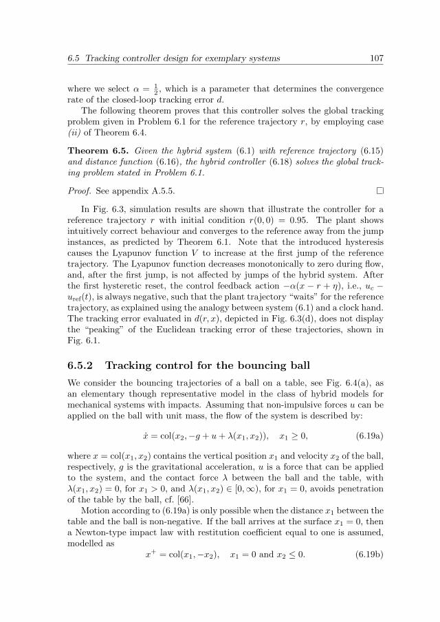
6.5 Tracking controller design for exemplary systems 107
where we select α = 12 , which is a parameter that determines the convergence
rate of the closed-loop tracking error d.The following theorem proves that this controller solves the global tracking
problem given in Problem 6.1 for the reference trajectory r, by employing case(ii) of Theorem 6.4.
Theorem 6.5. Given the hybrid system (6.1) with reference trajectory (6.15)and distance function (6.16), the hybrid controller (6.18) solves the global track-ing problem stated in Problem 6.1.
Proof. See appendix A.5.5.
In Fig. 6.3, simulation results are shown that illustrate the controller for areference trajectory r with initial condition r(0, 0) = 0.95. The plant showsintuitively correct behaviour and converges to the reference away from the jumpinstances, as predicted by Theorem 6.1. Note that the introduced hysteresiscauses the Lyapunov function V to increase at the first jump of the referencetrajectory. The Lyapunov function decreases monotonically to zero during flow,and, after the first jump, is not affected by jumps of the hybrid system. Afterthe first hysteretic reset, the control feedback action −α(x − r + η), i.e., uc −uref(t), is always negative, such that the plant trajectory “waits” for the referencetrajectory, as explained using the analogy between system (6.1) and a clock hand.The tracking error evaluated in d(r, x), depicted in Fig. 6.3(d), does not displaythe “peaking” of the Euclidean tracking error of these trajectories, shown inFig. 6.1.
6.5.2 Tracking control for the bouncing ball
We consider the bouncing trajectories of a ball on a table, see Fig. 6.4(a), asan elementary though representative model in the class of hybrid models formechanical systems with impacts. Assuming that non-impulsive forces u can beapplied on the ball with unit mass, the flow of the system is described by:
x = col(x2,−g + u+ λ(x1, x2)), x1 ≥ 0, (6.19a)
where x = col(x1, x2) contains the vertical position x1 and velocity x2 of the ball,respectively, g is the gravitational acceleration, u is a force that can be appliedto the system, and the contact force λ between the ball and the table, withλ(x1, x2) = 0, for x1 > 0, and λ(x1, x2) ∈ [0,∞), for x1 = 0, avoids penetrationof the table by the ball, cf. [66].
Motion according to (6.19a) is only possible when the distance x1 between thetable and the ball is non-negative. If the ball arrives at the surface x1 = 0, thena Newton-type impact law with restitution coefficient equal to one is assumed,modelled as
x+ = col(x1,−x2), x1 = 0 and x2 ≤ 0. (6.19b)
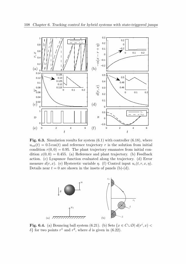
108 Chapter 6. Tracking control for hybrid systems with state-triggered jumps
0
0.2
0.4
0.6
0.8
1r,
x
rx
0
0.02
0.04
0.06
0.08
0.1
0.12
0.14
V 0 0.1 0.20.1150.12
0.1250.13
0.135
−0.2
−0.1
0
0.1
0.2
0.3
−α(x
−r
+η)
0 0.1 0.2
−0.2
0
0.2
0
0.1
0.2
0.3
0.4
0.5
d(r
,x)
0 0.1 0.2
0.46
0.48
0.5
0 2 4 6
0
1
η
t0 2 4 6
−0.5
0
0.5
t
u
uc
uref
(a)
(c)
(b)
(d)
(e) (f)
Fig. 6.3. Simulation results for system (6.1) with controller (6.18), whereuref(t) = 0.5 cos(t) and reference trajectory r is the solution from initialcondition r(0, 0) = 0.95. The plant trajectory emanates from initial con-dition x(0, 0) = 0.455. (a) Reference and plant trajectory. (b) Feedbackaction. (c) Lyapunov function evaluated along the trajectory. (d) Errormeasure d(r, x). (e) Hysteretic variable η. (f) Control input uc(t, r, x, η).Details near t = 0 are shown in the insets of panels (b)-(d).
(a)
g
u
x1
(b)
Fig. 6.4. (a) Bouncing ball system (6.21). (b) Sets x ∈ C∪D| d(ri, x) <δ for two points r1 and r2, where d is given in (6.22).
6.5 Tracking controller design for exemplary systems 109
We consider the following reference trajectory:
r(t) = col(τ − g2τ
2, 1− gτ), τ = t mod 2g , (6.20)
where mod denotes the modulus operator. This trajectory is a solution to(6.19) for initial conditions r(0, 0) = col(0, 1) and uref ≡ 0. In this example,we focus on the local tracking problem given in Problem 6.1 and design a staticcontrol law u = ud(t, r, x) such that the reference trajectory r is asymptoticallystabilised for the closed-loop plant dynamics. For trajectories near this referencetrajectory the contact force λ vanishes for almost all t, such that the trajectoriesare described by the system
x = F (t, x, u) := col(x2,−g + u), x ∈ C := [0,∞)× R, (6.21a)
x+ = G(x) := col(x1,−x2), x ∈ D := 0 × (−∞, 0]. (6.21b)
In order to define a tracking error measure d(r, x), we use the property that thevelocity x2 changes sign at impacts, and the position x1 is zero, see (6.21b).Hence, if we want to compare a reference state r with plant state x when one ofthem just experienced a jump, then the distance |x + r| is appropriate. Awayfrom jump instances, typically, the conventional distance |x−r| can be used. Todistinguish when the distance |x− r| or |x+ r| should be considered, we use theminimum of both, such that the novel distance measure is given by
d(r, x) = min(|x− r|, |x+ r|). (6.22)
To recognise that this distance function satisfies the conditions posed in Defini-tion 6.1, first, note that G(D)∩D = 0, such that Gk(x) = ∅,∀x ∈ C ∪D \ 0when k ≥ 2, implying that (∃k1, k2 ∈ N, such that Gk1(x) ∩ Gk2(r) 6= ∅) isequivalent to (x = r ∨ x = G(r) ∨ G(x) = r). Since G(x) = −x forx ∈ D, the condition (x = r ∨ x = G(r) ∨ G(x) = r) can be rewritten tox− r = 0∨x+ r = 0, such that d(r, x) = 0 directly follows and relation (6.6a) issatisfied. As required in (6.6b), for given r, β, the set x ∈ C ∪D| d(r, x) < βis compact, as it is the union of the bounded sets x ∈ C ∪ D| |x − r| < βand x ∈ C ∪ D| |x + r| < β. Since G(x) = −x for x ∈ D, relation (6.6c)holds, as d(r,G(x)) = d(r,−x) = min(|r − x|, |r + x|), which equals d(r, x). Ananalogue argument shows that (6.6d) holds. Since, in addition, d is continuous,the tracking error measure d(r, x) is compatible with the hybrid system (6.19).
In Fig. 6.4(b), the neighbourhoods x ∈ C ∪D| d(ri, x) < δ of two differentpoints ri, i = 1, 2, are shown. Essentially, the tracking error measure d allowsto compare a reference trajectory with a plant trajectory, “as if” both of themalready jumped. For example, in Fig. 6.4(b), the gray domain with positive x2
is considered close to r2, since r2 will experience a jump soon, and after thisjump, r2 will arrive in this domain.
We design a tracking control law u = ud(t, r, x) for system (6.21) using areasoning that exploits the design of the tracking error measure d in (6.22).

110 Chapter 6. Tracking control for hybrid systems with state-triggered jumps
Analogously to the design approach in the previous section, observe that d(r, x)in (6.22) is given by the minimum between the two functions, ρ1 = |x − r| andρ2 = |x + r|. When the trajectory x is sufficiently close to r and neither ofthem experiences a jump in the near future or past, then the tracking errord(r, x) given in (6.22) is given by ρ1 = |x− r|. Along solutions of the differentialequation (6.19a), this error could accurately be controlled towards zero using acontroller with PD-type feedback, given by
u1 = −[kp kd](x− r), (6.23)
where kp, kd > 0. Implementation of this controller yields the error dynamicsx1 − r1 = −kp(x1 − r1)− kd(x1 − r1), such that col(x1 − r1, x1 − r1) = col(0, 0)is an asymptotically stable equilibrium point of the flow dynamics with u givenin (6.23).
However, if either the reference trajectory or the plant just experienced ajump, d(r, x) as given in (6.22) is given by ρ2 = |x + r|. The continuous-timebehaviour of x + r is stable when the closed-loop dynamics satisfy x1 + r1 =−kp(x1 + r1)− kd(x1 + r1), which is obtained by selecting the controller as
u2 = 2g − [kp kd](x+ r), (6.24)
with kp, kd > 0. Based on these insights, we propose a controller that switchesbetween (6.23) and (6.24). To choose the partitioning of the state space whereeither (6.23) or (6.24) are applied, the following candidate Lyapunov functionV (r, x) is considered:
V (r, x) = min(Vd(r, x), Vm(r, x)), (6.25)
with
Vd(r, x) = 12 (x− r)TP (x− r), Vm(r, x) = 1
2 (x+ r)TP (x+ r), (6.26)
where a symmetric, positive definite matrix P and scalar c > 0 are chosen suchthat
ATP + PA ≺ −cP, (6.27)
with A =
[0 1−kp −kd
], where for symmetric and real matricesM,N , we adopt the
notation M ≺ 0 when M is negative definite, and M ≺ N when M−N ≺ 0. Forstrictly positive kp, kd, the matrix A is Hurwitz, which implies that such P andc exist, since [91, Theorem 4.6] implies that for any symmetric, positive definitematrix Q there exist a symmetric, positive definite P such that ATP+PA ≺ −Q,and c > 0 can be chosen sufficiently small, such that −Q ≺ −cP . Based onthe Lyapunov function candidate V , the following control law u = ud(t, r, x) isdesigned, such that ρ1 or ρ2 decreases along continuous-time solutions describedby (6.19a):
ud(t, r, x) =
−[kp kd](x− r), Vd ≤ Vm2g − [kp kd](x+ r), Vd > Vm.
(6.28)

6.6 Conclusion 111
In the next theorem we show that the control law (6.28) indeed solves thetracking problem formulated in Problem 6.1.
Theorem 6.6. Consider the bouncing ball system (6.21), tracking error d givenin (6.22) and reference trajectory r given in (6.20) for uref(t) ≡ 0. Applicationof the control law ud(t, r, x) as defined in (6.28), with Vd, Vm given in (6.26) andkp, kd > 0, to the hybrid system (6.21) makes the reference trajectory r asymptot-ically stable with respect to d. In addition, the set x ∈ C∪D| V (r(0, 0), x) ≤ Kis contained in the basin of attraction of r, where K is chosen to satisfy
K < min(t,j)∈dom r
V (r(t, j), 0). (6.29)
Proof. See Appendix A.5.6.
The control law ud(t, r, x) given in (6.26),(6.28) with [kp kd] = [1 0.5] and
P =
[2.25 0.50.5 2
]is applied to system (6.21) with g = 9.81. The trajectory
from the initial condition x(0, 0) = col(4, 3g4 ) is shown with the dashed line in
Fig. 6.5(a)-(b). Clearly, the hybrid trajectory x converges to r during flow,and the jump instances of r and x converge to each other. The Euclidean dis-tance |x − r| and the distance d(r, x) between both trajectories are shown inFig. 6.5(c) and (d), respectively. Although the Euclidean distance displays theunstable “peaking” behaviour, the tracking error expressed using the distanced(r, x) remains continuous over trajectories, and converges to zero. Hence, thelocal tracking problem as formulated in Problem 6.1 is solved, and the trajector-ies shown in Fig. 6.5(a) show desirable tracking behaviour. Indeed, as predictedby Theorem 6.1, |x − r| decreases to zero for r away from D ∪ G(D), wherer1 = 0.
Although the controller designs for the examples in Sections 6.5.1 and 6.5.2have been tailored to the specific examples, we care to highlight that we employeda common rationale for the controller design. First, the tracking error measured(r, x) is designed as the minimum of functions ρi, i = 1, 2, 3 corresponding to|x − r|, |x − G(r)|, |G(r) − x|, where the functions G are designed such thatG(x) = G(x) for x ∈ D. (For the bouncing ball example given in (6.21), thefunctions ρ2 and ρ3 coincide due to the structure of G and D.) Subsequently,for each function ρi, i = 1, 2, 3, a control law ui is designed that would stabilisethe set where ρi = 0 along flowing solutions. Finally, a Lyapunov candidatefunction is employed to determine which control law ui is applied in what partof the state space.
6.6 Conclusion
In this chapter, the problem of (global) tracking of time-dependent reference tra-jectories is studied for hybrid systems with state-triggered jumps. We formulated

112 Chapter 6. Tracking control for hybrid systems with state-triggered jumps
0
2
4
6
x1
r1
x1
−10
−5
0
5
x2
r2
x2
5
10
15
|x−
r|
0
2
4
d(r
,x)
0 2 4 6 8 10 12
0
10
20
ud
t
(a)
(b)
(c)
(d)
(e)
Fig. 6.5. (a),(b) Reference trajectory r and plant trajectory x of (6.21),where g = 9.81 and the control law (6.28) is applied with [kp kd] = [1 0.5].(c) Tracking error expressed in Euclidean distance |x − r|, (d) distancefunction d(r, x) given in (6.22) and (e) control input ud(t, r, x) for system(6.21).
the tracking problem in such a way that it corresponds to the intuitive notionof tracking for hybrid systems: the plant trajectories tend asymptotically to thereference trajectory, such that away from the time instances where the referencetrajectory jumps, the Euclidean tracking error becomes small. To formalise thisnotion of tracking, the tracking error is evaluated using a novel, non-Euclideandistance measure. It is shown in this chapter that such distance functions havethree advantages. First, it facilitates the formulation of a tracking problem thatis feasible for a large class of hybrid system, including mechanical systems withimpacts, and does not require the jumps of the plant to coincide with the jumpsof the reference trajectory. Second, the formulated tracking problem can beanalysed by evaluating Lyapunov functions along closed-loop trajectories, andis feasible for a large class of reference trajectories, which are not required to

6.6 Conclusion 113
be periodic. Third, as shown in the examples, the new tracking error measurecan be used to design controllers solving the tracking problem. Using exemplarysystems, including the well-known bouncing ball system, we illustrate that thetracking problem is feasible for hybrid systems with state-triggered jumps andthat the presented results support the design of tracking controllers for suchhybrid systems.
Further research should be directed to the development of a synthesis pro-cedure for generic hybrid systems that leads to, firstly, a tracking error measurethat is tailored to the hybrid system under study and, secondly, a control lawthat solves the tracking problem formulated in this chapter. The requirementson the distance measure and the stability analysis presented in this chapter formimportant stepping stones towards such a generic synthesis procedure.


Chapter 7
Conclusions andrecommendations
7.1 Conclusions
In this thesis, nonsmooth dynamical systems have been investigated and resultsare obtained in two domains. Firstly, in Part I of this thesis, the qualitativedynamical behaviour and the effect of parameter variations are discussed fornon-differentiable and discontinuous systems. Secondly, the tracking controlproblem for hybrid systems is studied in Part II.
In Part I, we discuss the qualitative dynamical behaviour and identify pos-sible bifurcations for two classes of nonsmooth systems, namely, for non-differ-entiable and discontinuous systems. In both system classes, the dynamics isdescribed by a differential equation that, away from some surfaces in the statespace, is a smooth vector field. If non-differentiable systems are considered,then the differential equation is continuous at the mentioned surfaces. Non-differentiable systems can describe, for example, control systems with actuatorsaturation or mechanical systems with one-sided flexibilities. In discontinuoussystems, the differential equation can be discontinuous at the mentioned surfaces.Discontinuous systems can be used, for example, to model mechanical systemswith friction, where the friction force is modelled with Coulomb’s friction law.
In this thesis, we present a procedure to analyse local bifurcations of thedynamics near equilibria in planar non-differentiable systems. For a class ofdiscontinuous systems describing mechanical systems with dry friction, sets ofnon-isolated equilibrium points are identified. Sufficient conditions are presentedfor the structural stability of the dynamics near such equilibrium sets, and non-smooth bifurcations are identified. Furthermore, the effect of a homoclinic orbit

116 Chapter 7. Conclusions and recommendations
from an endpoint of an equilibrium set has been investigated. When transversalhomoclinic orbits from such points exist, then a horseshoe-like limit set is foundthat exhibits features that are characteristic to nonsmooth systems.
In Part II, the tracking control problem for hybrid systems has been invest-igated. Hybrid systems show both continuous evolution in time and jumps ofthe states (i.e., discrete events). For example, hybrid systems can be used tomodel mechanical systems with impacts. Due to the jumps of hybrid systems,the standard tracking control problem for smooth dynamical systems can betoo restrictive. We have formulated a new tracking control problem, based ona non-Euclidean tracking error measure, and showed that this problem can besolved for a larger class of hybrid systems.
The contributions of this thesis are discussed in more detail below.
Local bifurcations of equilibria are studied in Chapter 2 for the class of planarnon-differentiable systems. For these systems, bifurcations may occur when, dueto a parameter variation, an equilibrium point arrives at a surface, or at the in-tersection of multiple surfaces, where the vector field is non-differentiable. Aprocedure is presented that can identify all limit sets that are created or des-troyed at such bifurcations. This procedure uses a local approximation of thesmooth vector fields that govern the dynamics away from the mentioned sur-faces, resulting in a conewise affine system that experiences the same bifurca-tion scenario as the local bifurcation of the non-differentiable system. With thepresented procedure, in an example, a new type of non-smooth bifurcation hasbeen identified.
In Chapters 3 and 4, a class of discontinuous dynamical systems has beenconsidered that represents mechanical systems with dry friction. In Chapter 3,it is shown that these systems generically have equilibrium sets, which are setsof non-isolated equilibrium positions that form intervals of curves in the statespace. We showed that, in general, local bifurcations near these equilibrium setscan only occur around the endpoints of these sets. Using this result, sufficientconditions are presented for the local structural stability near equilibrium setsin two-dimensional systems. In examples where these conditions are violated,local bifurcations are observed that change the dynamics near the equilibriumset.
In Chapter 4, for the same class of systems, homoclinic orbits are studiedthat emanate from an endpoint of an equilibrium set. A periodic perturbationof such systems induces a complex geometry of the sets of points converging to,or diverging from the endpoint of the equilibrium set. This geometry, whichis called the homoclinic tangle, is strongly affected by the discontinuity of thevector field. Using a return map, the dynamics near the homoclinic tangle isstudied, and a limit set is found whose geometry and dynamical behaviour areessentially different from those of the limit set that appears near homoclinictangles in smooth systems.
To attain a more detailed description of the newly found limit set, in Chap-

7.2 Recommendations 117
ter 5, we study the dynamics of a class of return maps with similar propertiesas the return map derived in Chapter 4. In particular, the considered mapsare continuous and non-invertible. It is shown that these maps have a limitset that is geometrically described as the Cartesian product of a Cantor setand a countable set of points. Furthermore, topologically conjugate symbolicdynamics are introduced, that are defined on a quotient space of infinite stringsof symbols. Using this symbolic dynamics, it is proven that the limit sets of theclass of maps considered in Chapter 5 are topologically transitive and contain aninfinite number of periodic orbits. Both of these properties are known to hold aswell for the Smale horseshoe map, which describes the dynamics near homoclinicorbits of smooth systems. For this reason, we argue that the non-invertible mapsconsidered in Chapter 5 are closely related to the Smale horseshoe map.
In Chapter 6, the tracking control problem for hybrid systems has been con-sidered. In this problem, a controller should be designed that forces a hybridsystem to follow a pre-described (jumping) reference trajectory asymptotically.In smooth dynamical systems, conventionally, the tracking controller is requiredto induce asymptotic stability, in the Euclidean error measure, of the referencetrajectory. However, if jumps of the system are state-triggered and the con-trol input does not affect these jumps, then the jump instants of the plant maybecome close to the jump instants of the reference trajectory, but these willgenerically not coincide. During the small time intervals of such a jump-timingmismatch, a peaking phenomenon is observed in the Euclidean tracking error,rendering asymptotic stability of the Euclidean tracking error infeasible. Thisproblem is addressed in Chapter 6 by reformulating the tracking problem suchthat it is not affected by the peaking phenomenon and still corresponds to anintuitively correct notion of tracking. The new tracking problem requires asymp-totic stability of the reference trajectory with respect to a non-Euclidean distancemeasure. This problem is less restrictive, and, consequently, for a larger classof hybrid systems, controllers can be designed that solve this tracking problem.We formulated sufficient conditions for the stability of a trajectory with respectto the new error measure, and, in two examples, we designed controllers solvingthe tracking problem.
7.2 Recommendations
In this section, recommendations are presented for further research on the dy-namics and control of nonsmooth systems. First, three recommendations aregiven that can be directly linked to the contents of the previous chapters. Sub-sequently, recommendations are formulated which have a broader scope.
• The effect of the discontinuous behaviour of dry friction on homoclinictangles has been discussed only briefly in Chapter 4. A mathematicallyrigourous description of this homoclinic tangle could perhaps be attained

118 Chapter 7. Conclusions and recommendations
when the lambda-lemma could be adapted such that it applies in the dis-continuous case discussed in Chapter 4. For smooth discrete-time systems,roughly speaking, the lambda-lemma states that a small disc that has atransversal intersection with the stable manifold of a hyperbolic equilib-rium point becomes arbitrarily close to the unstable manifold of this pointunder forward iterations of the map that defines the discrete-time system,cf. [127]. This result implies that a single transversal intersection betweenthe stable and unstable manifolds generates an infinite number of trans-versal intersections between these manifolds. Furthermore, if a transversalintersection is present, then the stable and unstable manifolds accumu-late on themselves, such that a homoclinic tangle is created. Hence, thelambda-lemma is instrumental to describe the geometry of the homoclinictangle in smooth systems. The numerical results presented in Section 5.2.1suggest that a result similar to the lambda-lemma does hold in an exem-plary system. Hence, we suggest to further investigate the dynamics nearthe points that are attracted to, or have diverged from, the endpoints ofthe equilibrium set. Such investigations may lead to a nonsmooth vari-ant of the lambda-lemma and could enable a rigourous description of thehomoclinic tangle discussed in Chapter 4.
• In Chapter 6, the tracking control problem for hybrid systems has beenstudied, and this problem is formulated using a non-Euclidean trackingerror measure. From a control perspective, it is desirable to developa synthesis procedure for classes of hybrid systems that, firstly, designsan error measure that is tailored to the hybrid system under study, andsecondly, designs a control law that solves the tracking problem presentedin Chapter 6.
• The results in Chapter 6 are formulated in the framework of [68]. However,the new formulation of the tracking control problem and the definition ofstability with respect to a non-Euclidean error measure can also be appliedin different hybrid system frameworks. If these ideas are transferred to theframework of measure differential inclusions, then tracking control prob-lems could be investigated for models of mechanical systems that use themore realistic contact and impact laws that are available in this framework.
• Most results on bifurcations and structural stability of nonsmooth systemsthat exist in the literature, including the results in Chapters 2, 4 and 5,have been derived only for systems with a low-dimensional (i.e. two, orthree-dimensional) state space. The development of dimension-reductiontechniques for non-differentiable and discontinuous systems would signific-antly increase the applicability of these results.
For smooth dynamical systems, dimension reduction can be achieved using,e.g., center manifolds [43] or normal hyperbolic invariant manifolds [57]. If

7.2 Recommendations 119
similar dimension reduction techniques could be attained for discontinuoussystems, then, next to the increased applicability of existing bifurcationresults, the dynamics of higher-dimensional nonsmooth models could bebetter understood. As a consequence, higher-dimensional nonsmooth sys-tems could also be more effectively used to model and analyse dynamicalphenomena in engineering, physics, biology or economy.
• The mathematical literature on bifurcations and structural stability innonsmooth systems has a strong emphasis on behaviour that is genericunder arbitrary perturbations of the right-hand side of the differentialequations. For various applications, this definition of generic behaviourexcludes physically relevant phenomena, such as non-isolated equilibriumpoints in mechanical systems with friction, as discussed in Chapter 3. Ifperturbations are considered that are physically relevant, but that preservesome of the qualitative properties of the vector field (e.g. perturbations pre-serving the kinematic relation between position and velocity in models ofmechanical systems), then results on structural stability and bifurcationscan be achieved that are important for a range of physical applications ofthe nonsmooth models. In this manner, bifurcation and structural stabil-ity results for restricted classes of perturbations can form an importantaddition to the existing theory of nonsmooth dynamical systems.
• The approximation of nonsmooth dynamical systems by smooth differen-tial equations (which is also called regularisation) may lead to importantinsights in the dynamical behaviour of the nonsmooth system. However,the limit sets of the approximating system, and its bifurcation diagram,can be qualitatively different from those of the nonsmooth dynamical sys-tem. In addition, approximating smooth models will not show the collapse(i.e. the loss of uniqueness) of trajectories that can occur in discontinuoussystems.
While acknowledging these fundamental differences between smooth andnonsmooth dynamical systems, we note that some of the main differencesbetween nonsmooth systems and their smooth approximations only mani-fest themselves when trajectories are considered over infinitely long timehorizons. For example, we expect that a set of non-isolated equilibriumpoints, that occurs in the class of systems discussed in Chapter 3, is rep-resented in a smooth approximation by a set in the state space where thevector field is very small. If trajectories in this set are considered on afinite time horizon, then little differences can be observed between thesetrajectories, and those of the discontinuous vector field.
Motivated by this example, we expect that if trajectories are only con-sidered on finite-time horizons, then the dynamics of nonsmooth systemscan be more directly linked with their smooth approximations. Using such
120 Chapter 7. Conclusions and recommendations
a link, various results that are obtained for smooth dynamical systems maybe of significant relevance in the domain of nonsmooth systems.
• The notion of stability of hybrid trajectories, as presented in Chapter 6to study the tracking control problem, can also be applied to differentproblems, e.g. in the fields of synchronisation, or observer design. In fact,the non-Euclidean distance measure introduced in Chapter 6 provides aversatile tool to study the differences between time-varying and jumpingtrajectories of hybrid systems. As such, this type of distance measures canalso be used, for example, to study the properties of numerical simulationroutines for hybrid systems.

Appendix A
Proofs and technical results
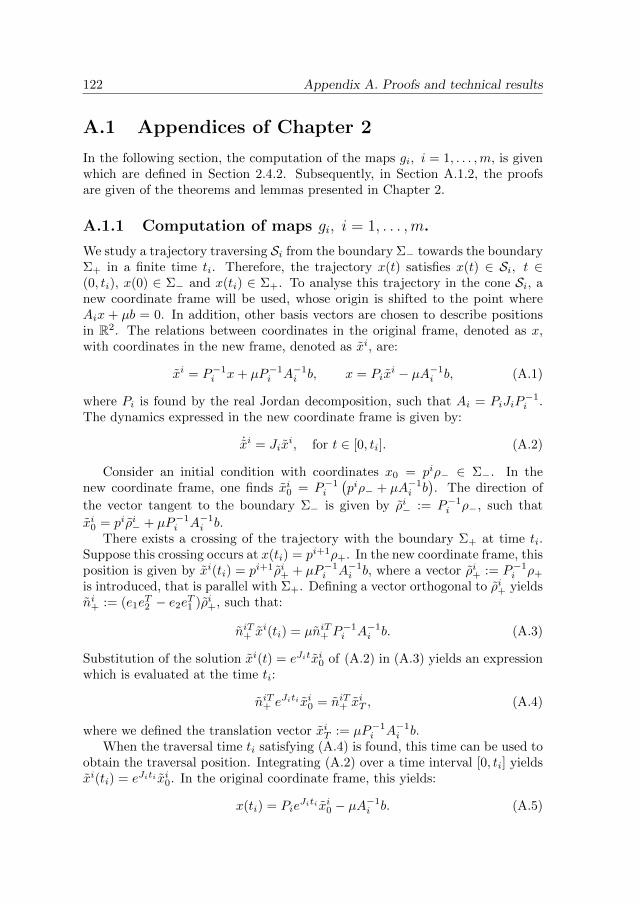
122 Appendix A. Proofs and technical results
A.1 Appendices of Chapter 2
In the following section, the computation of the maps gi, i = 1, . . . ,m, is givenwhich are defined in Section 2.4.2. Subsequently, in Section A.1.2, the proofsare given of the theorems and lemmas presented in Chapter 2.
A.1.1 Computation of maps gi, i = 1, . . . ,m.
We study a trajectory traversing Si from the boundary Σ− towards the boundaryΣ+ in a finite time ti. Therefore, the trajectory x(t) satisfies x(t) ∈ Si, t ∈(0, ti), x(0) ∈ Σ− and x(ti) ∈ Σ+. To analyse this trajectory in the cone Si, anew coordinate frame will be used, whose origin is shifted to the point whereAix + µb = 0. In addition, other basis vectors are chosen to describe positionsin R2. The relations between coordinates in the original frame, denoted as x,with coordinates in the new frame, denoted as xi, are:
xi = P−1i x+ µP−1
i A−1i b, x = Pix
i − µA−1i b, (A.1)
where Pi is found by the real Jordan decomposition, such that Ai = PiJiP−1i .
The dynamics expressed in the new coordinate frame is given by:
˙xi = Jixi, for t ∈ [0, ti]. (A.2)
Consider an initial condition with coordinates x0 = piρ− ∈ Σ−. In thenew coordinate frame, one finds xi0 = P−1
i
(piρ− + µA−1
i b). The direction of
the vector tangent to the boundary Σ− is given by ρi− := P−1i ρ−, such that
xi0 = piρi− + µP−1i A−1
i b.There exists a crossing of the trajectory with the boundary Σ+ at time ti.
Suppose this crossing occurs at x(ti) = pi+1ρ+. In the new coordinate frame, thisposition is given by xi(ti) = pi+1ρi+ + µP−1
i A−1i b, where a vector ρi+ := P−1
i ρ+
is introduced, that is parallel with Σ+. Defining a vector orthogonal to ρi+ yieldsni+ := (e1e
T2 − e2e
T1 )ρi+, such that:
niT+ xi(ti) = µniT+ P−1i A−1
i b. (A.3)
Substitution of the solution xi(t) = eJitxi0 of (A.2) in (A.3) yields an expressionwhich is evaluated at the time ti:
niT+ eJiti xi0 = niT+ xiT , (A.4)
where we defined the translation vector xiT := µP−1i A−1
i b.When the traversal time ti satisfying (A.4) is found, this time can be used to
obtain the traversal position. Integrating (A.2) over a time interval [0, ti] yieldsxi(ti) = eJiti xi0. In the original coordinate frame, this yields:
x(ti) = PieJiti xi0 − µA−1
i b. (A.5)

A.1 Appendices of Chapter 2 123
Substitution of the time ti satisfying (A.4) in (A.5) forms a map gi : Di ⊂Σ− → Ri ⊂ Σ+, describing the position of the crossing position of the trajectoryx(t), t > 0, x(0) ∈ Di with Σ+, such that x(ti) = gi(x(0)). The map gi willbe computed by distinguishing the following three cases:
Case 1: If Ai has complex eigenvalues, then Ji =
[ai −ωiωi ai
], where ai and ωi
are real and ωi > 0. Hence, eJit = eait[cos(ωit) − sin(ωit)sin(ωit) cos(ωit)
]. Herewith, (A.4)
yields:eaiti cos(ωiti)n
iT+ xi0 + eaiti sin(ωiti)ρ
iT+ xi0 = niT+ xiT . (A.6)
This equation can be solved with a numerical solver to obtain the time ti. Thistime yields the position:
x(ti) = −eaiti sin(ωiti)Pi(e1e
T2 − e2e
T1
)xi0 + eaiti cos(ωiti)Pix
i0 − µA−1
i b.
(A.7)
Case 2: If Ai has two real eigenvalues λai and λbi whose eigenvectors are distinct,
then Ji =
[λai 00 λbi
]. Using eJit = eλaite1e
T1 + eλbite2e2, we obtain: xi(t) =
eλaite1eT1 x
i0 + eλbite2e
T2 x
i0, such that (A.4) becomes:
eλaiti niT+ e1eT1 x
i0 + eλbiti niT+ e2e
T2 x
i0 = niT+ xiT , (A.8)
that can be solved with a numerical solver to obtain the smallest time ti > 0.Evaluating (A.5) on this time yields:
x(ti) = eλaitPie1eT1 x
i0 + eλbitPie2e
T2 x
i0 − µA−1
i b. (A.9)
Case 3: If Ai has two equal real eigenvalues λai with geometric multiplicity 1,
then Ji =
[λai 10 λai
]and eJit = eλait
[1 t0 1
]. Substituting this expression in (A.4)
yields:eλaiti niT+ xi0 + tie
λaiti niT+ e1eT2 x
i0 = niT+ xiT . (A.10)
When the smallest ti > 0 satisfying (A.10) is found with a numerical solver, thiscan be substituted in (A.5), yielding:
x(ti) = eλaitiPixi0 + tie
λaitiPie1eT2 x
i0 − µA−1
i b. (A.11)
A.1.2 Proofs
Proof of Theorem 2.1. First we prove the existence of at least one equilibriumpoint. For this purpose, the index of a point and the index of a Jordan curveare introduced. Next, we will prove the second part of the theorem.
Let ∆θ be the total change in the angle θ that the vector f(x) makes withsome fixed direction as x traverses a Jordan curve J once in the positive direction.

124 Appendix A. Proofs and technical results
Recall from [74] that a Jordan curve is defined as a topological image of acircle, i.e. J is an x-set of points x = x(t), a ≤ t ≤ b, where x(t) is continuous,x(a) = x(b) and x(s) 6= x(t), for a ≤ s < t < b. Define the index of J withrespect to f as If (J) := ∆θ
2π .
Define the index of an isolated equilibrium point P with respect to f asthe index of any Jordan curve encircling P , and no other equilibrium points.This index will be denoted by If (P ). For certain equilibria, the index is known;If (P ) = 1 if P is a hyperbolic node or focus and If (P ) = −1 if P is a hyperbolicsaddle.
According to Theorem 4.4, p. 400, [46], since C is a periodic orbit, If (C) = 1.The periodic orbit C is a Jordan curve, such that Theorem 4.1, p. 398, [46] yieldsthat C encircles at least one equilibrium point. This proves the first statementof the theorem.
Suppose that all equilibrium points P1, . . . Pm that are encircled by the closedorbit are hyperbolic. Application of Corollary 2, p. 400, [46] yields that the sumof indices of these equilibria equals one, i.e. If (C) =
∑mi=1 If (Pi) = 1. The
value of the indices of a node, focus and saddle imply, that there must be anodd number 2n+ 1 of equilibria, of which n are saddles and n+ 1 are nodes orfoci.
Proof of Lemma 2.3. Three cases are distinguished according to the eigenvaluesof the matrix A, that describes the dynamics y = Ay in region S. The exist-ence of a visible eigenvector, corresponding to a real eigenvalue, implies that alleigenvalues of A ∈ R2×2 are real.
In the first case, the eigenvalues of A are equal and this eigenvalue has geo-metric multiplicity two. The trajectories inside S converge to the origin sincey = Ay yields y(t) = eλty0, ∀y0 ∈ S, where λ < 0.
In the second case, the matrix A has an eigenvalue λ < 0 with algebraicmultiplicity two and geometric multiplicity one. Trajectories starting in S canbe written as y(t) = PeJtP−1y0 = eλt(y0 + tPe1e
T2 P−1y0) as long as y(τ) ∈
S ∀τ ∈ [0, t], where the Jordan canonical form A = PJP−1 is used, with J =
λ(e1eT1 + e2e
T2 ) + e1e
T2 , e1 :=
(1 0)T
and e2 :=(0 1)T
. Consequently, theorientation of the vector eλt(y0 + tPe1e
T2 P−1y0) converges, for t → ∞, to the
orientation of Pe1, which is the eigenvector corresponding to eigenvalue λ. Withλ < 0, either convergence of the trajectory to the origin is obtained, or thetrajectory leaves S in finite time.
In the third case, the matrix A has two distinct eigenvalues λa < 0 andλb ∈ R \ λa. Trajectories in the region S are either positioned on the equi-librium, such that y(t) = 0, ∀t > 0, or the trajectories can be written asy(t) = PeJtP−1y0 = Pe1e
T1 P−1y0e
λat + Pe2eT2 P−1y0e
λbt, ∀y0 ∈ S as long asy(τ) ∈ S, ∀τ ∈ [0, t], where the Jordan canonical form A = PJP−1 is used, withJ = λae1e
T1 +λbe2e
T2 and y0 ∈ S. The eigenvectors of A are given by the vectors
va = Pe1 and vb = Pe2. The trajectory y(t) converges to either Iva = y ∈

A.1 Appendices of Chapter 2 125
R2|y = cva, c ∈ (0,∞) when λa > λb or Ivb = y ∈ R2|y = cvb, c ∈ (0,∞)when λa < λb. If trajectories converge to the set Ivk, k = a, b, corresponding toa visible eigenvector, i.e. Ivk ∈ S, k = a, b, they will approach the origin, sincethe corresponding eigenvalue λk < 0, k = a, b. Otherwise, they will leave theregion S in finite time.
Proof of Lemma 2.4. When S is a halfline, the vector field Ay is pointing outof S, since otherwise, all y ∈ S \ 0 are eigenvectors, that are visible. Everynonempty closed cone S ⊂ R2 that is not a halfline can be written as theunion of two nonempty closed convex cones S1 and S2 that do not contain asubspace of R2, i.e. S = S1 ∪ S2, where these cones intersect only at the halflineΣ12 = S1 ∩ S2. Due to the assumption in Lemma 2.4, both regions Sj , j = 1, 2,and the boundary Σ12 do not contain an eigenvector of A.
According to Theorem 3 of [4], for any y0 ∈ Sj , j = 1, 2, with y0 6= 0,there exists a time t1 ≥ 0 such that eAt1y0 6∈ Sj . Trajectories can traversethe boundary Σ12 only in one direction. Therefore, trajectories from a pointy0 ∈ Sj leave S in a finite time, possibly after traversing the other cone Sk, k ∈1, 2, k 6= j.
Proof of Lemma 2.5. Necessity is trivial. To prove sufficiency of the stabilityrequirements, we will prove that for every trajectory y(t), with initial conditiony0 ∈ R2 \ 0, there exist a finite time tf and closed cone Sk, such that y(t) ∈Sk,∀t > tf . Subsequently, we will prove that the trajectories converge to theorigin for t→∞.
Consider the trajectory from any initial condition y0 ∈ R2 \ 0. When y0 isinside a cone S containing no visible eigenvectors, Lemma 2.4 guarantees thatthe trajectory will leave this cone in a finite time. When y0 is inside a cone Scontaining visible eigenvectors, then, according to Lemma 2.3, trajectories mayconverge to the origin asymptotically and remain in this cone. In that case,choose tf = 0. Otherwise, they will leave the cone S in a finite time.
Trajectories can traverse a boundary Σi,i+1 = y ∈ R2|y = cρi,i+1, c ∈(0,∞) only in one direction, either from Si to Si+1 or vise versa, since thevector field f(y) on y = cρi,i+1 is given by y = cAiρi,i+1 and c > 0. Thismeans that possibly after leaving or traversing of some regions, all trajectorieswill arrive at a cone Sk containing a visible eigenvector and remain there for allt > tf . Here, tf is the sum of the finite time it took to escape the first region, andthe finite times for the traversal of regions without visible eigenvectors. Sincethese times are all finite according to Lemmas 2.3 and 2.4, the sum of these,which is defined as tf , is also finite.
By Lipschitz continuity, the trajectory y(t) remains bounded for t ∈ [0, tf ].Subsequently, it remains in a specific cone Sk for all t > tf , where Sk containsa visible eigenvector. Hence, Lemma 2.3 guarantees asymptotic stability of theorigin.

126 Appendix A. Proofs and technical results
Proof of Theorem 2.6. When visible eigenvectors are present, then necessity andsufficiency of (i) is given in Lemma 2.5. In absence of visible eigenvectors,necessity of (ii) is proven by contradiction. Let T be the period time of thespiralling motion of (2.5), as given in [4]. When Λ ≥ 1, then a trajectoryfrom y0 ∈ Σm1 visits the sequence of positions y(kT ) = Λky0, k = 1, 2, . . .,contradicting asymptotic stability.
Sufficiency of (ii) can be obtained by proving that all trajectories will crossthe boundary Σm1 in finite time. After this finite time, the contraction propertyof the return map yk+1 = Λyk, with Λ < 1, implies asymptotic stability.
For trajectories starting with initial conditions positioned in one of the re-gions Si, i = 1, . . . ,m, according to Lemma 2.4, there exists a finite timet1 ∈ [0,∞), such that the trajectory is not in the region Si. Since no statejumps can exist in (2.5), the trajectory will therefore cross a boundary Σi,i+1
in a finite time ts ∈ [0, t1]. Each boundary can only be traversed in one dir-ection. Therefore, only a finite number of regions Si can be traversed, beforeΣm1 is reached in a finite time. In this finite time, the trajectory does not growunbounded since the right-hand side of (2.5) is globally Lipschitz.
After the trajectory has reached Σm1 for the first time, the trajectory con-verges to the origin in a spiralling motion, as described by the return mapyk+1 = Λyk, due to the fact that Λ < 1. Herewith, sufficiency of (ii) isproven.
Proof of Theorem 2.8. To prove the theorem, first, a scaling law for conewiselinear systems is presented in Lemma A.1. Second, a relationship between tra-jectories of the conewise affine system with µ 6= 0 and conewise linear systemswith µ = 0 is given in Lemma A.2. Using that result, Theorem 2.8 is proven.
Lemma A.1. Consider two trajectories of the continuous, conewise linear sys-tem:
y =f(y), (A.12)
f(y) :=Aiy, y ∈ Si, i = 1, . . . ,m, (A.13)
where Si, i = 1, . . . ,m, are cones. Let y0 and y0 be two initial conditions, thatsatisfy y0 = cy0, c ∈ [0,∞). If y(t) is a trajectory for the system with y(0) = y0,then y(t) = cy(t) is a trajectory emanating from y(0) = y0.
Proof. The proof is omitted for the sake of brevity and follows from the obser-vation that f(y) is homogeneous of degree 1.
Lemma A.2. Consider the continuous, conewise affine system given in (2.3),with constant µ 6= 0. Suppose this system does not contain visible eigenvectors.Define a Poincare section for this system at the moments where the trajectoryx(t) traverses Σm1 with a specified direction (i.e. either from Sm to S1 or viseversa). Define the return map M : DM ⊂ Σm1 → IM ⊂ Σm1, such that M(xk)

A.1 Appendices of Chapter 2 127
denotes the position of the first crossing of x(t), t > 0, for the initial conditionx(0) = xk ∈ Σm1.Construct a conewise linear system (A.12) by setting µ = 0 in (2.3). Let Λ forthe conewise linear system (A.12) be defined by (2.8), (2.9), (2.10) and (2.12).The following two statements hold for the trajectories x(t) of the conewise affinesystem (2.3):
(i) When Λ < 1, there exists an xF ∈ Σm1 such that ‖M(xk)‖ < ‖xk‖, ∀xk ∈R := x ∈ Σm1| ‖x‖ ≥ ‖xF ‖.
(ii) When Λ > 1, there exists an xF ∈ Σm1 such that ‖M(xk)‖ > ‖xk‖, ∀xk ∈R := x ∈ Σm1| ‖x‖ ≥ ‖xF ‖.
Proof. An analytical expression for xF is obtained as follows. The conewiseaffine system (2.3) is considered as a perturbed conewise linear system, whereµb is considered as the perturbation. Using the fact that the system is globallyLipschitz, the difference between the trajectory x(t) of the conewise affine systemand the trajectory y(t) of the conewise linear system (A.12) can be bounded fora given time period. A trajectory of y(t) from y0 ∈ Σm1 is studied, that encirclesthe origin and crosses the boundary Σm1 after one spiralling motion. We will usean initial condition y0, with ‖y0‖ large enough, such that the trajectories y(t)and x(t) emanating from this initial position will encircle the origin and traversethe boundary Σm1, independent of the direction of the bounded perturbation.To find such an initial condition y0 we first study an arbitrary initial positiony0 ∈ Σm1, for which the trajectory y(t) of (A.12) is followed during one spirallingperiod.
Let T be the period time of the spiralling motion of (A.12), as given in [4].Consider a trajectory y(t), t ∈ [0, T ], of (A.12) with an arbitrary initial conditiony0 ∈ Σm1 \ 0 at time t = 0. From the stability analysis of the system (A.12),we obtain y(T ) = Λy0, where Λ is defined in (2.8), (2.9), (2.10) and (2.12).
Define the open set C(y0) as:
C(y0) :=
(Sm ∪ Σm1 ∪ S1) ∩ y ∈ R2|0 < ρTm1y < ‖y0‖,
if Λ < 1,(Sm ∪ Σm1 ∪ S1) ∩ y ∈ R2|ρTm1y > ‖y0‖,
if Λ > 1.
(A.14)
Note that ρm1 is a unit vector. The set C(y0) is shown in Fig. A.1. Withoutloss of generality, assume that for all y ∈ Σm1 \ 0 the vector field f(y) of(A.12) is pointing in direction of S1. Here, no generality is lost, since f(·) ishomogeneous, Σm1 \0 is a halfline from the origin and the regions Si can berenumbered such that f(y) is pointing in direction of S1 for all y ∈ Σm1 \ 0.Since y(T ) ∈ Σm1 and f(y(T )) is pointing in direction of S1, one can concludethat there exist small times τ−, τ+ ∈ (0, T ) such that the trajectory y(t) satisfies

128 Appendix A. Proofs and technical results
(a) Λ < 1 (b) Λ > 1
Fig. A.1. Graphical representation of the conditions (A.18)-(A.20) forΛ < 1 and Λ > 1. The set C(y0) is shown as the dashed region. Note thatthe domain around y(t), t ∈ [T − τ−, T + τ+] is contained in C(y0).
the following three conditions:
y(t) ∈ C(y0),∀t ∈ [T − τ−, T + τ+], (A.15)
y(T − τ−) ∈ C(y0) ∩ Sm, (A.16)
y(T + τ+) ∈ C(y0) ∩ S1. (A.17)
Here, the following facts are used; the trajectory y(t) is continuous in time,the point y(T ) ∈ C(y0) and the trajectory traverses Σm1 from Sm towards S1 atthe time instant t = T . Since C(y0), Sm and S1 are open sets, there exists anε ∈ (0,∞), such that for all vectors δ, with ‖δ‖ ≤ ε the conditions
y(t) + δ ∈ C(y0),∀t ∈ [T − τ−, T + τ+], (A.18)
y(T − τ−) + δ ∈ C(y0) ∩ Sm, (A.19)
y(T + τ+) + δ ∈ C(y0) ∩ S1, (A.20)
are satisfied. These conditions are illustrated in Fig. A.1. A new initial con-dition y0 = ky0, with k a positive constant, is chosen for the system (A.12).Application of Lemma A.1 yields that y(t) = ky(t). We introduce ζ = kδ, suchthat combination of the conditions (A.18)-(A.20) with definition (A.14) yields:
y(t) + ζ ∈ C(y0),∀t ∈ [T − τ−, T + τ+], (A.21)
y(T + τ−) + ζ ∈ C(y0) ∩ Sm, (A.22)
y(T + τ+) + ζ ∈ C(y0) ∩ S1, (A.23)
for the trajectory y(t) with initial condition y0 = ky0 and for all ζ with ‖ζ‖ ≤ kε.Now, consider the affine term of (2.3), i.e. µb, as a constant disturbance of
the system (A.12). We study the trajectory x(t) of (2.3) and the trajectory y(t)
A.1 Appendices of Chapter 2 129
of (A.12), both with the same initial condition xk0 = y0 = ky0 at t = 0. Sincesystem (2.3) is globally Lipschitz with Lipschitz constant L, Theorem 3.4 in [91]can be applied, yielding
‖y(t)− x(t)‖ ≤ |µ|L
(eL(T+τ+) − 1
),∀t ∈ [0, T + τ+], (A.24)
where µ is given in (2.3), ‖b‖ = 1 is used, T the period of the spiralling motion
of (A.12) and τ+ is introduced above. If we choose y0 ∈ R :=y0 ∈ R2|y0 =
ky0, k ≥ |µ|εL
(eL(T+τ+) − 1
), with y0 and ε introduced above, then (A.24)
yields ‖x(t)− y(t)‖ ≤ kε, ∀t ∈ [0, T + τ+] and (A.21)-(A.23) yield:
x(t) ∈ C(xk0),∀t ∈ [T − τ−, T + τ+], (A.25)
x(T − τ−) ∈ C(xk0) ∩ Sm, (A.26)
x(T + τ+) ∈ C(xk0) ∩ S1, (A.27)
where we used xk0 = y0. From these conditions we conclude that the continuoustrajectory x(t) of (2.3) crosses Σm1 ∩C(xk0) at a time tc ∈ (T − τ−, T + τ+). Thedefinition of the map M in Lemma A.2 yields M(xk0) = x(tc) ∈ Σm1 ∩ C(xk0),where x(t) denotes the trajectory of (2.3) with initial condition xk0 . For Λ < 1,the intersection Σm1 ∩ C(xk0) equals x ∈ Σm1|‖x‖ ∈ (0, ‖xk0‖). For Λ > 1, theintersection Σm1 ∩ C(xk0) equals x ∈ Σm1|‖x‖ > ‖xk0‖.
Consequently, the set R, as presented under (A.24), satisfies the conditionsof the lemma. The set R can be written as R = x ∈ Σm1| ‖x‖ ≥ ‖xF ‖, with
xF :=|µ|εL
(eL(T+τ+) − 1
)y0, y0 ∈ Σm1 \ 0. (A.28)
Hence, for Λ < 1, we obtain ‖M(x0)‖ < ‖x0‖, ∀x0 ∈ R = x ∈ Σm1| ‖x‖ ≥‖xF ‖. For Λ > 1, we obtain ‖M(x0)‖ > ‖x0‖, ∀x0 ∈ R = x ∈ Σm1| ‖x‖ ≥‖xF ‖.
Using Lemma A.2, we will now prove Theorem 2.8. Consider a trajectoryfrom the initial condition x0 ∈ R = x ∈ Σm1| ‖x‖ ≥ ‖xF ‖, with xF derivedin Lemma A.2, and assume Λ 6= 1. Define the return map M on Σm1 accordingto Lemma A.2, and choose xF as given in that lemma. The return map of thetrajectory through the point x0 satisfies ‖M(x0)‖ 6= ‖x0‖.
It remains to be proven that the trajectory from M(x0) can not return tox0 after the first crossing of Σm1 at position M(x0). Without loss of generality,suppose the trajectory traverses Σm1 from Sm towards S1 at t = 0. The vectorfield (2.3) on the boundary Σm1 can be described by x = A1x + µb, x ∈ Σm1,which is autonomous and affine. Hence, all trajectories traversing [x0,M(x0)]cross this line from Sm to S1. Since the trajectory from M(x0) can not crosshis own trajectory or [x0,M(x0)], it not return to x0. No closed orbit can existthat contains a point x0 ∈ R.

130 Appendix A. Proofs and technical results
Proof of Theorem 2.9. Consider a visible eigenvector v ∈ Si, i = 1, . . . ,m, cor-responding to the real eigenvalue λu of a system matrix Ai. Define a unitvector ni,i+1 normal to the boundary Σi,i+1 and a unit vector ni−1,i normal tothe boundary Σi−1,i, where both vectors point towards Si. This implies thatSi = x ∈ R2|xTni,i+1 > 0 ∧ xTni−1,i > 0.
Now, we will prove that there exists a scalar cH ∈ [0,∞), such that thehalfline H = x ∈ R2|x = −µA−1
i b + cv, c ∈ [cH ,∞) is included completelyin Si, that is the closure of Si. Taking the inner product of the vectors x =−µA−1
i b + cv, c ∈ (0,∞) with ni−1,i and ni,i+1, we find that xTni−1,i > 0 if
c >µnTi−1,iA
−1i b
nTi−1,ivand xTni,i+1 > 0 if c >
µnTi,i+1A−1i b
nTi,i+1v. Both denominators are
nonzero and positive, since the visible eigenvector v is not contained in either ofthe boundaries Σi−1,i or Σi,i+1, as stated in the theorem, and v ∈ Si accordingto Definition 2.3. Consequently, the set H is contained in the closure of Si, i.e.
H ⊂ Si, when cH = max(µnTi−1,iA
−1i b
nTi−1,iv,µnTi,i+1A
−1i b
nTi,i+1v).
Consider a trajectory of (2.3) with initial position x0 ∈ H. Any position inH can be written as x = −µA−1
i b + cv, such that substitution in (2.3) yieldsx = cAiv. However, since v is an eigenvector, we obtain x = cλuv. This vectorfield is tangent to the halfline H. This implies, that trajectories can only enteror leave the halfline H at x = −µA−1
i b + cHv, the end point of the halfline.When the vector field at this point is into (out of) H, then H is a positively(negatively) invariant set.
Uniqueness of solutions of (2.3) excludes closed orbits inside the halfline H.In addition, a closed orbit can not traverse H, since in that case, the closed orbitshould enter and leave H. This is not possible, since H is either a positively ornegatively invariant set. No closed orbits can exist that either are contained inH, or contain a point in H.
Proof of Theorem 2.10. The proof of this theorem is given in two parts. InPart 1, the theorem is proven for all ν ∈ N \ 0. Subsequently, in Part 2, thecase ν = 0 is discussed.
Part 1In this part we will first discuss the existence of equilibria for ν 6= 0, subsequentlytheir local stability properties are discussed. Let J ⊆ 1, . . . , m contain theindices, such that the domains Di, i ∈ J contain the origin. According to As-sumption 2.1, Fi(0, 0) = 0, ∀i ∈ J . With Assumption 2.4, we can apply theImplicit Function Theorem, cf. [122], which yields that for each i ∈ J locallythere exists a smooth path xi,1(ν), that satisfies Fi(xi,1(ν), ν) = 0. Note thatthis path may be positioned outside Di. When xi,1(ν) ∈ Di for given ν ∈ N ,then an equilibrium of (2.1) exists in this domain. Assumption 2.5 excludes thepossibility that there exists an equilibrium in the domain Di for ν ∈ N whenDi is a cusp-shaped region at the origin. (Note that a cusp-shaped region isnot represented by a cone in (2.3)). Therefore, we may restrict ourselves to the

A.1 Appendices of Chapter 2 131
paths of possible equilibria xi,1(ν), i ∈ 1, . . . ,m ⊆ J .Differentiating Fi(xi,1(ν), ν) = 0 with respect to ν, we obtain with Assump-
tions 2.2 and 2.4:
∂Fi∂ν
∣∣∣∣(x,ν)=(0,0)
+∂Fi∂x
∣∣∣∣(x,ν)=(0,0)
∂xi,1(ν)
∂ν
∣∣∣∣(x,ν)=(0,0)
= 0,
∂xi,1(ν)
∂ν
∣∣∣∣(x,ν)=(0,0)
= −A−1i b. (A.29)
To prove the first statement of the theorem for ν, µ 6= 0, without loss ofgenerality we may assume there exists a positive ν∗, such that xi,1(ν) ∈ Di forall ν ∈ (0, ν∗) for a given i ∈ 1, . . . ,m, where an open set Di is chosen since we
adopted Assumption 2.5. This implies that∂xi,1(ν)∂ν
∣∣∣(x,ν)=(0,0)
= −A−1i b ∈ Di,
and since Di is locally approximated by Si and µ = ν > 0, we obtain −µA−1i b ∈
Si, for µ > 0. In combination with the fact that equilibria of (2.3) are positionedon xi,2(µ) = −µA−1
i b, we obtain the following result: when (2.1) contains anequilibrium in Di for an i ∈ 1, . . . ,m and ν in a range (0, ν∗), then (2.3)contains an equilibrium point in Si for all µ > 0.
To prove the converse statement, we note that with Assumption 2.5, all pathsof equilibria of (2.3) will be positioned in a cone Si, i = 1, . . . ,m. Therefore,we assume without loss of generality that (2.3) contains an equilibrium pathxi,2(µ) ∈ Si for µ > 0 and given i ∈ 1, . . . ,m, such that fi(xi,2(µ), µ) = 0.Solving this equation yields xi,2(µ) = −µA−1
i b ∈ Si, ∀µ > 0. Using (A.29),
we obtain:∂xi,1(ν)∂ν
∣∣∣(x,ν)=(0,0)
∈ Si, where xi,1(ν) denotes a path such that
Fi(xi,1(ν), ν) = 0 holds. The domain Di is locally approximated by Si, such
that we have:∂xi,1(ν)∂ν
∣∣∣(x,ν)=(0,0)
∈ Di. Since xi,1(ν) is a smooth path and Di is
an open set, there exists a ν∗ > 0 such that xi,1(µ) ∈ Di,∀ν ∈ (0, ν∗).For ν = µ 6= 0, the final statement of Theorem 2.10, which states that the
stability properties of the equilibria of (2.1) and (2.3) are identical, is obtainedfrom the Andronov-Pontryagin condition, cf. Theorem 2.5 of [95]. Without lossof generality, we assume there exists an equilibrium of (2.1), that follows anequilibrium path xi,1(ν) ∈ Di for ν ∈ (0, ν∗) ⊂ N , ν∗ > 0 with i ∈ 1, . . . ,m.We define Fi(x, ν) := Fi(x−xi,1(ν), ν) for ν ∈ (0, ν∗), which is a smooth function,
such that x = Fi(x, ν) describes the dynamics of (2.1) in a neighbourhood N(ν)near the equilibrium. For each ν ∈ (0, ν∗), N(ν) 3 0 is chosen such, that for allx ∈ N(ν), x+ xi,1(ν) lies inside Di.
According to the Andronov-Pontryagin condition the system x = Fi(x, ν) isstructurally stable in N(ν). Therefore, there exists an ε > 0 such that for allvector fields Gi that satisfy
supx∈N(ν)
(‖Fi(x)−Gi(x)‖+
∥∥∥∥∂Fi∂x− ∂Gi
∂x
∥∥∥∥) ≤ ε, (A.30)
132 Appendix A. Proofs and technical results
the systems x = Gi(x) and x = Fi(x) are topologically equivalent. ChoosingGi(x) = Aix, and observing that Fi(x, ν) and xi,1(ν) are smooth functions
satisfying xi,1(0) = 0 and ∂Fi∂x
∣∣∣(x,ν)=(0,0)
= ∂Gi∂x
∣∣(x,ν)=(0,0)
= Ai, we can choose ν
and N(ν) small enough such that (A.30) is satisfied. Since x = Gi(x) describesthe dynamics in the neighbourhood of an equilibrium of (2.3), the systems (2.1)and (2.3) near their equilibria are locally topologically equivalent for ν ∈ (0, ν∗)when ν∗ is chosen small enough. In addition, the stability properties of theequilibria of (2.3) and (2.1) are equal. Hence, the theorem is proven for the caseν 6= 0.
Part 2In this part, we will prove the theorem for the case ν = 0. Existence of anisolated equilibrium at the origin of (2.1) for ν = 0 is given by Assumption 2.1.By construction, an equilibrium at the origin exist in (2.3) for µ = 0, which isisolated since all matrices Ai are invertible, cf. Assumption 2.4. It remains tobe proven that the local stability properties of the equilibrium at the origin of(2.1) with ν = 0 and (2.3) with µ = 0 are equal.
By Assumption 2.4, either a stable or unstable manifold of this equilibriumexist, or all trajectories near an equilibrium of (2.1) encircle this point. There-fore, we will study both cases, yielding Lemmas A.3 and A.4, respectively.
We study manifolds of the non-differentiable systems (2.1) and (2.3) similarto the stable and unstable manifolds of nodes and saddle points in smooth dy-namical systems. However, we allow these manifolds to be defined only in adomain Si, i = 1, . . . ,m or Di, i = 1, . . . , m.
Lemma A.3. Under Assumptions 2.1 and 2.4, the equilibrium at the origin of(2.1) with ν = 0 has a stable (unstable) manifold if and only if the equilibrium atthe origin of (2.3) with µ = 0 has a stable (unstable) manifold, that is tangentto the manifold of (2.1) at the origin.
Proof. First, we will prove the necessity part of the lemma. By Assumption2.1, an equilibrium exists at the origin for the non-differentiable system (2.1).Assume this equilibrium of (2.1) has a stable (unstable) manifold C that em-anates from the origin towards a domain Di, i = 1, . . . , m. We distinguish twocases. In Case I, we will prove that this manifold of (2.1) is represented in (2.3)when the manifold emanates from the origin towards a domain Di, i = 1, . . . ,m,that does not form a cusp. Subsequently, we will prove this statement when themanifold emanates into a cusp-shaped domain in Case II, which, after a possiblerenumbering of the domains Di, can be denoted with Dn, n ∈ m+ 1, . . . , m.
To prove necessity in Case I, we assume that the manifold C ∈ Di, i =1, . . . ,m, is not positioned in a cusp of boundaries near the origin. Then, thedomain Di in (2.1) is represented by the cone Si in (2.3). When C is emanatingtangentially to a boundary Cij of (2.1), then we choose the index i such thaton the intersection of the manifold C with a neighbourhood of the origin, the

A.1 Appendices of Chapter 2 133
dynamics of system (2.1) is described by x = Fi(x, 0). This implies that thereexists a λ such that ∂Fi
∂x
∣∣(x,ν)=(0,0)
r = λr, where r is the vector tangent to C
at the origin, with the direction chosen to satisfy r ∈ Di. Note that λ < 0(λ > 0) for the stable (unstable) manifold. Since Ai is defined as ∂Fi
∂x
∣∣(x,ν)=(0,0)
,
Ai therefore has eigenvector r. Since Di is locally approximated with Si, theeigenvector r is visible in Si. This implies that the set c := x ∈ R2 : x =sr, s ∈ [0,∞) is a manifold of the conewise affine system (2.3), on which thedynamics is given by x = Aix = λx, such that a stable (unstable) manifold of(2.3) corresponds to a stable (unstable) manifold of (2.1).
To prove necessity in Case II, we assume that the manifold C is eman-ating from the origin towards a cusp of boundaries into a domain Dn, n ∈m + 1, . . . , m of (2.1), and r is the vector pointing into this cusp from theorigin. Then, there exists a λ such that ∂Fn
∂x
∣∣(x,ν)=(0,0)
r = λr. Without loss
of generality, we assume that we do not have two or more adjoining cusp-shaped regions. Note that λ < 0 (λ > 0) for the stable (unstable) mani-fold. Since the vector field of (2.1) is continuous at each boundary Cij , we
observe that ∂Fi∂x ρCij (x) =
∂Fj∂x ρCij (x),∀x ∈ Cij , where ρCij (x) denotes a vec-
tor tangent to Cij at the point x. Therefore, ∂Fn∂x
∣∣(x,ν)=(0,0)
r = λr implies
that ∂Fi∂x
∣∣(x,ν)=(0,0)
r =∂Fj∂x
∣∣∣(x,ν)=(0,0)
r = λr, with the indices i, j ∈ 1, . . .mchosen such that the domains Di and Dj have boundaries tangent to the cuspat the origin, although the domains Di and Dj do not form a cusp at the origin.
Since Ai and Aj are, respectively, defined as ∂Fi∂x
∣∣(x,ν)=(0,0)
and∂Fj∂x
∣∣∣(x,ν)=(0,0)
,
both Ai and Aj have eigenvector r. The domains Di and Dj are locally ap-proximated with, respectively, Si and Sj , such that the eigenvector r is visibleand lies on the boundary Σij between Si and Sj . This implies that the setc := x ∈ R2 : x = sr, s ∈ [0,∞) is a manifold of the conewise affine sys-tem (2.3), on which the dynamics is given by x = Aix = Ajx = λx, such that astable (unstable) manifold of (2.3) corresponds to the stable (unstable) manifoldof (2.1). In both cases, the necessity part of the lemma is obtained.
Now, we will prove the sufficiency part of the lemma by assuming that thereexists a stable (unstable) manifold c ∈ Si, i = 1, . . . ,m, of the system (2.3).Since the dynamics in this cone is given by x = Aix, we can denote this manifoldwith c = x ∈ R2 : x = sr, s ∈ [0,∞), where r ∈ Si is an eigenvector ofAi. Let λ be the eigenvalue corresponding to this eigenvector. Since c is astable (unstable) manifold, we obtain λ < 0 (λ > 0). Again, two cases aredistinguished. First, we will study the case where c is positioned in an opencone Si, subsequently we will prove the sufficiency part of the theorem in case cis positioned on a boundary.

134 Appendix A. Proofs and technical results
To prove sufficiency in the first case, we assume that the stable (unstable)manifold c is positioned in an open cone Si. Then the Hartman-Grobman The-orem, [74], guarantees that the system x = Fi(x, 0) locally has the same stableand unstable manifolds as the system x = Aix. Therefore, the vector fieldFi(x, 0) satisfies ∂Fi
∂x
∣∣(x,ν)=(0,0)
r = λr. Since the trajectories of (2.3) in the cone
Si coincide with the trajectories of x = Aix and the trajectories of (2.1) in thedomain Di coincide with the trajectories of x = Fi(x, 0), the non-differentiablesystem (2.1) has a stable (unstable) manifold corresponding to c if λ < 0 (λ > 0).
To prove sufficiency in the second case, we assume the stable (unstable)manifold c of (2.3) lies on a boundary Σij . Recall that ρij denotes the vec-tor tangent to Σij , pointing towards this ray. Let K ⊆ 1, . . . , m denote theset of indices, such that Dn has a boundary tangent to Σij at the origin ifand only if n ∈ K. (The domain Dn may or may not be a cusp-shaped re-gion). We assumed the existence of a stable (unstable) manifold c of (2.3) ona boundary Σij . This implies that there exists a λ < 0 (λ > 0) such thatAiρij = λρij = ∂Fi
∂x
∣∣(x,ν)=(0,0)
ρij . For the sake of contradiction, suppose (2.1)
has no stable (unstable) manifold tangent to Σij . Then ∀n ∈ K, ∀λn < 0 (λn >0) : ∂Fn
∂x
∣∣(x,ν)=(0,0)
ρij 6= λnρij . However, since F (x, ν) is continuous, we obtain∂Fi∂x
∣∣(x,ν)=(0,0)
ρij = ∂Fn∂x
∣∣(x,ν)=(0,0)
ρij , ∀n ∈ K. Hence, Ai = ∂Fi∂x
∣∣(x,ν)=(0,0)
has
no eigenvalue λ < 0, (λ > 0) with the eigenvector ρij , contradicting the exist-ence of a stable (unstable) manifold with eigenvalue λ in (2.3). A contradictionis obtained, such that (2.1) has a stable (unstable) manifold, which is tangentto Σij at the equilibrium. In both cases, the sufficiency part of the lemma isproven.
Lemma A.4. Under Assumptions 2.1, 2.4, and 2.6, all trajectories of (2.1)with ν = 0 in a neighbourhood around the equilibrium at the origin are spirallingaround the origin and converge towards the origin for t→∞ (t→ −∞) if andonly if all trajectories of (2.3) with µ = 0 are spiralling around the origin andconverge to the origin for t→∞ (t→ −∞).
Proof. First we prove the sufficiency part of the statement, subsequently the ne-cessity part of the statement is proven. Assume a spiralling motion exists in thesystem (2.3). Since system (2.3) is Lipschitz continuous, the time-reversed sys-tem can be studied, and since, in addition, the chosen coordinate frame may bemirrored along a coordinate axis, we may assume, without loss of generality, thatthe spiralling motion is counter clockwise and trajectories of (2.3) are convergingto the origin for t→∞. We consider a trajectory of (2.3) starting at t = 0 froma point x0 which is positioned on the positive vertical axis. There exists a timeT such that the trajectory x(t) of (2.3) encircles the origin O once and returnsto a point x(T ) on the interval of the line segment [O, x0]. We will comparethe trajectories x(t) of (2.3) with x(t) of (2.1), where both are starting fromx(0) = x(0) = x0. With the same reasoning as used in the proof of Theorem 2.8,
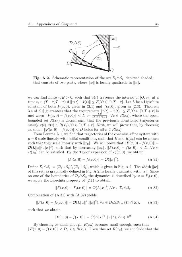
A.1 Appendices of Chapter 2 135
Fig. A.2. Schematic representation of the set Di4Si, depicted shaded,that consists of two parts, where ‖w‖ is locally quadratic in ‖x‖.
we can find finite τ, E > 0, such that x(t) traverses the interior of [O, x0] at atime tc ∈ (T − τ, T + τ) if ‖x(t)− x(t)‖ ≤ E,∀t ∈ [0, T + τ ]. Let L be a Lipschitzconstant of both F (x, 0), given in (2.1) and f(x, 0), given in (2.3). Theorem3.4 of [91] guarantees that the requirement ‖x(t)− x(t)‖ ≤ E,∀t ∈ [0, T + τ ] ismet when ‖F (x, 0) − f(x, 0)‖ < D := LE
eL(T+τ)−1, ∀x ∈ R(x0), where the open,
bounded set R(x0) is chosen such that the previously mentioned trajectoriessatisfy x(t), x(t) ∈ R(x0),∀t ∈ [0, T + τ ]. Next, we will prove that, by choosingx0 small, ‖F (x, 0)− f(x, 0)‖ < D holds for all x ∈ R(x0).
From Lemma A.1, we find that trajectories of the conewise affine system withµ = 0 scale linearly with initial conditions, such that E and R(x0) can be chosensuch that they scale linearly with ‖x0‖. We will prove that ‖F (x, 0)−f(x, 0)‖ =O(L‖x‖2, ‖x‖2), such that by decreasing ‖x0‖, ‖F (x, 0) − f(x, 0)‖ < D, ∀x ∈R(x0) can be satisfied. By the Taylor expansion of Fi(x, 0), we obtain:
‖Fi(x, 0)− fi(x, 0)‖ = O(‖x‖2). (A.31)
Define Di4Si := (Di∪Si)\ (Di∩Si), which is given in Fig. A.2. The width ‖w‖of this set, as graphically defined in Fig. A.2, is locally quadratic with ‖x‖. Sinceon one of the boundaries of Di4Si, the dynamics is described by x = Fi(x, 0),we apply the Lipschitz property of (2.1) to obtain:
‖F (x, 0)− Fi(x, 0)‖ = O(L‖x‖2),∀x ∈ Di4Si. (A.32)
Combination of (A.31) with (A.32) yields:
‖F (x, 0)− fi(x, 0)‖ = O(L‖x‖2, ‖x‖2),∀x ∈ Di4Si ∪ (Di ∩ Si), (A.33)
such that we obtain
‖F (x, 0)− f(x, 0)‖ = O(L‖x‖2, ‖x‖2),∀x ∈ R2. (A.34)
By choosing x0 small enough, R(x0) becomes small enough, such that‖F (x, 0)− f(x, 0)‖ < D, x ∈ R(x0). Given this set R(x0), we conclude that the
136 Appendix A. Proofs and technical results
trajectory x(t) from x0 ∈ R(x0), starting from the positive vertical axis, crossesthe interior of the line [O, x0] in the time interval [T − τ, T + τ ]. Consequently,the non-differentiable system (2.1) exhibits a spiralling motion, and trajectoriesof (2.1) in the neighbourhood R(x0) do converge to the origin for t→∞, when‖x0‖ is chosen small enough.
The necessity part of the statement is equivalent with the statement thatthe absence of a stable (unstable) spiralling motion of (2.3) with µ = 0 excludesa stable (unstable) spiralling motion of (2.1) with ν = 0. To prove the latterstatement, assume the conewise linear system (2.3) with µ = 0 does not exhibitspiralling motion, converging to the origin for t → ∞ (t → −∞). ConsideringAssumptions 2.4 and 2.6, system (2.3) should either exhibit spiralling motionconverging to the origin for t → −∞ (t → ∞), or should contain visible ei-genvectors. In the first case, the spiralling motion, converging to the origin fort → −∞ (t → ∞), implies that in a neighbourhood of the origin, a spirallingmotion of (2.1) with ν = 0 exist, and trajectories converge to the origin fort → −∞ (t → ∞). This follows directly from the sufficiency part of the proof.In case visible eigenvectors exist in (2.3) with µ = 0, Lemma A.3 guarantees thata manifold exist in (2.1) for ν = 0, emanating from the origin. This manifoldexcludes a spiralling motion of (2.1) for ν = 0. Hence, we have proven that theabsence of a stable (unstable) spiralling motion of (2.3) with µ = 0 excludes astable (unstable) spiralling motion of (2.1) with ν = 0.
Given Assumption 2.4 an equilibrium is unstable when either an unstablemanifold exist, or a diverging spiralling motion occurs. An equilibrium point islocally asymptotically stable when a converging spiralling motion exist or whena stable manifold exist, and no unstable manifolds. Trajectories encircling anequilibrium, which are not converging to this point for t→∞ or t→ −∞, are,in a neighbourhood around the origin, excluded by Assumption 2.6. Therefore,application of Lemma A.3 guarantees that at ν = µ = 0, the stability proper-ties of the equilibrium at the origin of (2.1) and (2.3) are equal when visibleeigenvectors exist in (2.1). When no visible eigenvectors exist in (2.1), then thestability properties of the equilibria at the origin of (2.1) and (2.3) are equalaccording to Lemma A.4.
Proof of Theorem 2.11. To prove Theorem 2.11, first we will introduce a newcoordinate system, and derive the technical Lemma A.5 for the obtained system.Subsequently, in Lemma A.6 we will state an intermediate result about thenumber of limit cycles, which will be used to prove the theorem.
In a new coordinate system z = xµ , defined for µ 6= 0, the conewise affine
system (2.3) is represented as:
z = f(z), (A.35)
f(z) = Aiz + b, z ∈ Si. (A.36)

A.1 Appendices of Chapter 2 137
Clearly, this transformation does not change the existence and stability of limitsets of the conewise affine system. Expressing (2.1) in the coordinates z = x
ν ,defined for ν 6= 0, we obtain:
z =F (z, ν), (A.37)
F (z, ν) =Fi(z, ν) :=1
νFi(νz, ν), z ∈ Di, (A.38)
where Di := z ∈ R2|z = xν , x ∈ Di.
For the difference between f(z) in (A.36) and F (z, ν) in (A.38), we obtainthe following lemma.
Lemma A.5. Consider F (z, ν) as given in (A.38) and f(z) as given in (A.36).For every domain R(ν) := z ∈ R2|‖z‖ ≤ c|ν|, c > 0, and for all D > 0 thereexists a ν > 0, such that
‖F (z, ν)− f(z)‖ ≤ D, ∀ν ∈ (−ν, ν), ∀z ∈ R(ν). (A.39)
Proof. We observe that
‖Fi(z, ν)− fi(z)‖ =1
νO(ν2‖z‖2, ν2‖z‖, ν2), (A.40)
= O(ν3c2, ν2c, ν), ∀z ∈ R(ν), (A.41)
since fi is a first-order approximation of Fi, such that ‖Fi(x, ν) − fi(x, ν)‖ =O(‖x‖2, ν‖x‖, ν2).
The set Di4Si := (Di∪Si)\ (Di∩Si) is given in Fig. A.2. The width ‖w‖ ofthis set, as graphically defined in Fig. A.2, is locally quadratic with ‖x‖. At leastat one of the boundaries of Di4Si, we know that Fi = Fj , due to continuityof the vector field F , where j ∈ 1, . . . , m is chosen such that Dj adjoins Di.Hence, we obtain ‖Fj(x, ν)−Fi(x, ν)‖ = O(L‖w‖) = O(L‖x‖2), where (2.1) and(2.3) both have a Lipschitz constant L. This implies:
‖Fj(z, ν)− Fi(z, ν)‖ = O(ν3Lc2),∀z ∈ (Di4Si) ∩ Si) ∩R(ν), (A.42)
where Di4Si := (Di ∪ Si) \ (Di ∩ Si).Note that the state space can be partitioned as: R2 =
⋃i=1,...,m
(¯Di ∩ Si
)∪⋃
i=1,...,m
(Di4Si
). This implies that combination of (A.41) and (A.42) yields
‖F (z, ν) − f(z)‖ = O(ν3c2, ν2c, ν, ν3Lc2), ∀z ∈ R(ν), such that for all D > 0and bounded domain R(ν) defined in the lemma, we can find a ν 6= 0 such that
‖F (z, ν)− f(z)‖ ≤ D, ∀ν ∈ (−ν, ν),∀z ∈ R(ν).
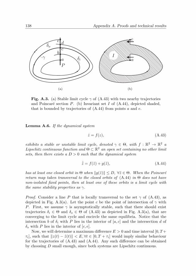
138 Appendix A. Proofs and technical results
(a) (b)
Fig. A.3. (a) Stable limit cycle γ of (A.43) with two nearby trajectoriesand Poincare section P . (b) Invariant set I of (A.44), depicted shaded,that is bounded by trajectories of (A.44) from points a and e.
Lemma A.6. If the dynamical system
z = f(z), (A.43)
exhibits a stable or unstable limit cycle, denoted γ ∈ Θ, with f : R2 → R2 aLipschitz continuous function and Θ ⊂ R2 an open set containing no other limitsets, then there exists a D > 0 such that the dynamical system
˙z = f(z) + g(z), (A.44)
has at least one closed orbit in Θ when ‖g(z)‖ ≤ D, ∀z ∈ Θ. When the Poincarereturn map taken transversal to the closed orbits of (A.44) in Θ does not havenon-isolated fixed points, then at least one of these orbits is a limit cycle withthe same stability properties as γ.
Proof. Consider a line P that is locally transversal to the set γ of (A.43), asdepicted in Fig. A.3(a). Let the point c be the point of intersection of γ withP . First, we assume γ is asymptotically stable, such that there should existtrajectories δi ∈ Θ and δo ∈ Θ of (A.43) as depicted in Fig. A.3(a), that areconverging to the limit cycle and encircle the same equilibria. Notice that theintersection b of δi with P lies in the interior of [a, c] and the intersection d ofδo with P lies in the interior of [c, e].
Now, we will determine a maximum difference E > 0 and time interval [0, T+τi], such that ‖z(t) − z(t)‖ < E, ∀t ∈ [0, T + τi] would imply similar behaviourfor the trajectories of (A.43) and (A.44). Any such difference can be obtainedby choosing D small enough, since both systems are Lipschitz continuous.
A.1 Appendices of Chapter 2 139
The following argument is similar as in the proof of Theorem 2.8. Let T bechosen such that z(T ) = b when z(0) = a. We choose a small τi > 0 such thatthe trajectory z(t) from z(0) = a satisfies ‖z(t)− b‖ < min(‖a− b‖, ‖c− b‖),∀t ∈[T − τi, T + τi]. When the trajectory z(t), t ∈ [0, T + τi] of (A.43) from z(0) = aand z(t), t ∈ [0, T + τi] of (A.44) from z(0) = a satisfy ‖z(t) − z(t)‖ ≤ Ei, fort ∈ [0, T + τi], with Ei > 0 small enough, then the trajectory z(t) from z(0) = atraverses the interior of [a, c] in a time interval t ∈ (T − τi, T + τi).
In a similar fashion, we can derive τo and Eo, such that when the trajectoryz(t), t ∈ [0, T +τo] of (A.43) from z(0) = b and z(t), t ∈ [0, T +τo] of (A.44) fromz(0) = e satisfy ‖z(t) − z(t)‖ ≤ Eo, t ∈ [0, T + τo], with Eo > 0 small enough,then the trajectory z(t) from z(0) = e traverses the interior of [c, e] in a timeinterval t ∈ (T − τo, T + τo).
Now, let E = min(Ei, Eo). When L is a Lipschitz constant of f(x), The-orem 3.4 of [91] implies ‖z(t) − z(t)‖ ≤ E, t ∈ [0,max(T + τi, T + τo)] issatisfied for the trajectories from z(0) = z(0) = a and z(0) = z(0) = e,when E = D
L
(eLmax(T+τi,T+τo) − 1
), such that choosing a positive D ≤ D :=
LEe(Lmax(T+τi,T+τo))−1
renders E > 0 small enough. In that case, the orbits of
(A.43) and (A.44) from the point a both show, during one rotation, a divergingspiralling motion with respect to the origin. Similarly, the orbits of (A.43) and(A.44) from the point e show a converging spiralling motion during one rotation.
Since (A.43) is Lipschitz continuous, when a and e are chosen close enough toc and a positive D ≤ D is chosen small enough, the function nTp ˙z is of constantsign on the line segment [a, e], where a normal vector np of P is introduced. Thisimplies that the domain I is a positively invariant set, with I bounded by twotrajectories of (A.44) and two line segments of [a, e], as depicted in Fig. A.3(b).In addition, the points a and e can be chosen such, that the domain I doesnot contain equilibria of (A.44) and all trajectories of (A.44) remain in Θ fort ∈ [0, T + τ ], with small τ > 0. Therefore, the Poincare-Bendixson theorem,see [74], guarantees the existence of a closed orbit in I for system (A.44).
Since I is a positively invariant set, a stable limit set of (A.44) exists inI. This follows from studying the return map of the perturbed system (A.44),which should be monotonous, to allow uniqueness of solutions in reverse time.Denoting the return map of the perturbed system with M , we observe that‖M(a)‖ > ‖a‖ and ‖M(e)‖ < ‖e‖. Since ‖a‖ < ‖e‖, this implies that themonotonous function xk+1 = M(xk) has to cross the line xk+1 = xk from‖M(xk)‖ > ‖xk‖ towards ‖M(xk)‖ < ‖xk‖ in the interval xk ∈ [a, e]. When nonon-isolated fixed points in this return map can occur, as stated in the lemma,then the perturbed system (A.44) exhibits a limit cycle which is asymptoticallystable. The case of an unstable limit cycle follows analogously by studying thetime-reversed systems.
Using this lemma, Theorem 2.11 can be proven. By Assumption 2.7, allclosed orbits of (2.1) are limit cycles. At given system parameter ν, for each
140 Appendix A. Proofs and technical results
stable or unstable limit cycle γi, i = 1, . . . , l, of system (2.1), we can define anopen set Ri(ν) 3 γi, containing no other limit sets. We apply the coordinatetransformation z = x
|ν| , relating (2.3) to (A.35) and (2.1) to (A.37), since we
assumed µ = ν. Using Assumption 2.8, all limit cycles γi, i = 1, . . . , l, of (2.1)are represented in the system (A.37), such that (A.37) contains the same numberl of limit cycles, denoted γi, i = 1, . . . l, and the stability properties of γi and γicorrespond for i = 1, . . . l.
Combination of Assumption 2.7 and Lemma A.6 yields that, since Ri(ν) isan open set and the system (2.1) is Lipschitz continuous, there exists a D > 0such that when
‖F (z, ν)− f(z)‖ ≤ D,∀z ∈ Ri(ν), (A.45)
holds, then ki limit cycles of (A.35) exists in Ri(ν), of which at least one hasthe same stability properties as γi. According to Lemma A.5, a neighbourhoodN of ν = 0 exists, such that condition (A.45) is satisfied. Applying the reversedtransformation x = |µ|z, we obtain ki limit cycles of the conewise affine system(2.3), of which at least one has the same stability properties as γi.
The proof of the theorem is concluded by proving ki = 1, ∀i = 1, . . . , l, whichis proven by contradiction. Suppose that there exists a domain Ri(ν) with ki ≥ 2stable or unstable limit cycles γi,j , j = 1, . . . , ki, existing in the system (2.3)in the domain Ri(ν), i = 1, . . . , l. For all these sets γi,j , j = 1, . . . , ki, we canfind non-overlapping domains Ri,j(ν) ⊂ Ri(ν), j = 1, . . . , ki, containing onlyone limit cycle. Using the same reasoning as above, we obtain that therefore,every set Ri,j(ν) contains a limit cycle of the non-differentiable system (2.1),implying Ri(ν) contains at least ki limit cycles. By construction however, Ri(ν)contains only one such set, yielding a contradiction. Therefore, ki = 1 for alli ∈ 1, . . . , l. Hence, the numbers of stable or unstable limit cycles of (2.1) and(2.3) are equal. In addition, their stability properties are equal.
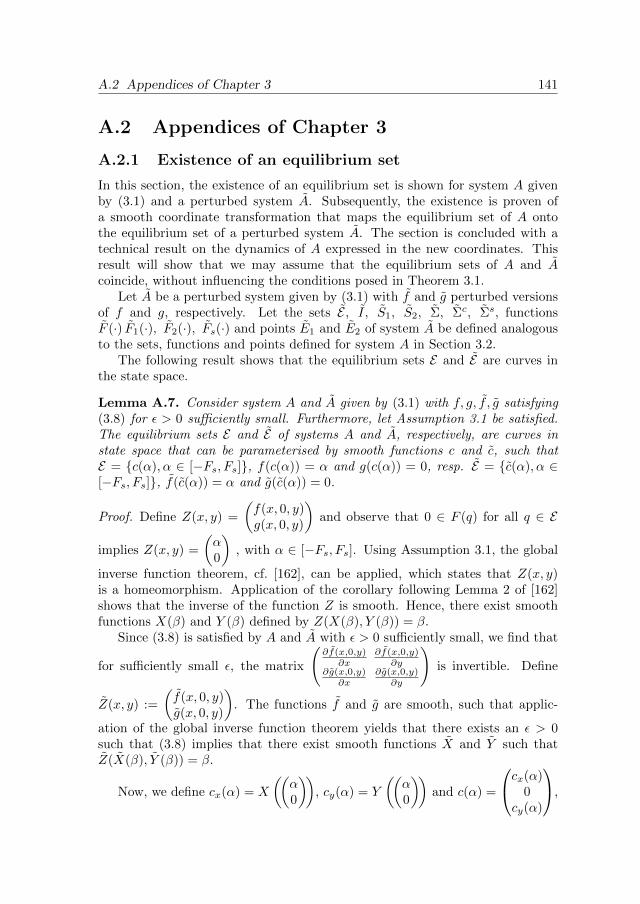
A.2 Appendices of Chapter 3 141
A.2 Appendices of Chapter 3
A.2.1 Existence of an equilibrium set
In this section, the existence of an equilibrium set is shown for system A givenby (3.1) and a perturbed system A. Subsequently, the existence is proven ofa smooth coordinate transformation that maps the equilibrium set of A ontothe equilibrium set of a perturbed system A. The section is concluded with atechnical result on the dynamics of A expressed in the new coordinates. Thisresult will show that we may assume that the equilibrium sets of A and Acoincide, without influencing the conditions posed in Theorem 3.1.
Let A be a perturbed system given by (3.1) with f and g perturbed versionsof f and g, respectively. Let the sets E , I, S1, S2, Σ, Σc, Σs, functionsF (·) F1(·), F2(·), Fs(·) and points E1 and E2 of system A be defined analogousto the sets, functions and points defined for system A in Section 3.2.
The following result shows that the equilibrium sets E and E are curves inthe state space.
Lemma A.7. Consider system A and A given by (3.1) with f, g, f , g satisfying(3.8) for ε > 0 sufficiently small. Furthermore, let Assumption 3.1 be satisfied.The equilibrium sets E and E of systems A and A, respectively, are curves instate space that can be parameterised by smooth functions c and c, such thatE = c(α), α ∈ [−Fs, Fs], f(c(α)) = α and g(c(α)) = 0, resp. E = c(α), α ∈[−Fs, Fs], f(c(α)) = α and g(c(α)) = 0.
Proof. Define Z(x, y) =
(f(x, 0, y)g(x, 0, y)
)and observe that 0 ∈ F (q) for all q ∈ E
implies Z(x, y) =
(α0
), with α ∈ [−Fs, Fs]. Using Assumption 3.1, the global
inverse function theorem, cf. [162], can be applied, which states that Z(x, y)is a homeomorphism. Application of the corollary following Lemma 2 of [162]shows that the inverse of the function Z is smooth. Hence, there exist smoothfunctions X(β) and Y (β) defined by Z(X(β), Y (β)) = β.
Since (3.8) is satisfied by A and A with ε > 0 sufficiently small, we find that
for sufficiently small ε, the matrix
(∂f(x,0,y)
∂x∂f(x,0,y)
∂y∂g(x,0,y)
∂x∂g(x,0,y)
∂y
)is invertible. Define
Z(x, y) :=
(f(x, 0, y)g(x, 0, y)
). The functions f and g are smooth, such that applic-
ation of the global inverse function theorem yields that there exists an ε > 0such that (3.8) implies that there exist smooth functions X and Y such thatZ(X(β), Y (β)) = β.
Now, we define cx(α) = X
((α0
)), cy(α) = Y
((α0
))and c(α) =
cx(α)0
cy(α)
,

142 Appendix A. Proofs and technical results
such that Z(cx(α), cy(α)) =(α, 0
). The curve c(·) is a parameterisation of E ,
such that E = q ∈ Rn : q = c(α), α ∈ [−Fs, Fs]. Analogously, a parameterisa-tion c(·) of E can be constructed.
Using this lemma, a map is constructed that maps the equilibrium set E ofA onto the equilibrium set E of A.
Lemma A.8. Consider system A and A given by (3.1) with f, g, f , g satisfying(3.8) for ε > 0 sufficiently small. Furthermore, let Assumption 3.1 be satisfied
and let ∂g∂y
∣∣∣p
be invertible for all p ∈ E. There exists a smooth map He =
Hxe
H xe
Hye
with smooth inverse in a neighbourhood of E, such that Hx
e = Hxe (x) and H x
e =dHxedx x, that maps E onto E. Furthermore, for any δ > 0 there exists an ε > 0
such that for any system A for which (3.8) holds for that ε, the resulting map He
satisfies ‖He(q)−q‖ < δ and ‖∂He∂q −I‖ < δ, where I denotes the n−dimensionalidentity matrix.
Proof. In this proof, the map He is constructed as follows. Using Lemma A.7,it will be shown that the equilibrium sets E and E can be parameterised asfunctions of x and x, respectively. Using this parameterisation, a map He isconstructed that maps the curve E onto E .
Consider the parameterisations c(·) and c(·) of E and E , respectively, as givenin Lemma A.7. In order to construct a mapHe that is defined in a neighbourhoodof E , we extend c(α) and c(α) such that they are defined in a neighbourhoodof a closed set α ∈ [α1, α2], with α1 < −|Fs| and α2 > |Fs|, which is possibleaccording to the extension lemma, see [100].
Let c(α) =
cx(α)0
cy(α)
and c(α) =
cx(α)0
cy(α)
. Differentiating the defining
expressions f(cx(α), 0, cy(α)) = α and g(cx(α), 0, cy(α)) = 0 with respect to α
yields ∂f∂x
dcxdα + ∂f
∂ydcydα = 1, and ∂g
∂xdcxdα + ∂g
∂ydcydα = 0, which should be satisfied
at the equilibrium set. Since both equations should be satisfied, dcxdα 6= 0 has
to hold along the equilibrium curve, since dcxdα = 0 and the first equation would
requiredcydα 6= 0, such that the second equation could not be satisfied, as ∂g
∂y
is invertible. Smoothness of g and c imply that one can pick α1 < −|Fs| and
α2 > |Fs| sufficiently close to −Fs and Fs, such that dcxdα
∣∣α6= 0 and ∂g
∂y
∣∣∣c(α)
is invertible for all α ∈ (α1, α2). The function cx(α) is smooth, such that therelation dcx
dα
∣∣α6= 0 implies that the inverse function theorem can be applied,
which yields that there exists a smooth inverse c−1x (x) defined on the interval
x ∈ cocx(α1), cx(α2). Furthermore, dcxdα 6= 0 implies that cx is either monoton-ously increasing or decreasing, such that the x-variables of E are positioned in

A.2 Appendices of Chapter 3 143
cocx(−Fs), cx(Fs). Now, let y = Ψ(x) := cy(c−1x (x)) denote the y−coordinate
such that the equilibrium set E can be parameterised as follows:
E = q ∈ Rn : q =(x 0 ΨT (x)
)T, x ∈ cocx(−Fs), cx(Fs). (A.46)
We observe that c−1x (x) is defined on the interval x ∈ cocx(α1), cx(α2) and
cy(α) is defined on (α1, α2). Hence, the map Ψ(x) is defined in a neighbourhoodof cocx(−Fs), cx(Fs).
To construct a function Ψ(·) for the equilibrium set E analogous to Ψ(·), first
we will prove that ∂g∂y
∣∣∣p
is invertible for p ∈ E if ε is sufficiently small. Since the
functions f, g, f , and g are smooth and satisfy Assumption 3.1 and (3.8), theinverse function theorem implies that for each ε1 > 0 there exists an ε > 0 suchthat for each p satisfying
(p2 f(p) g(p)T
)=(0 α 0
)there exists a p, such that(
p2 f(p) g(p)T)
=(0 α 0
)and ‖p− p‖ < ε1. Hence, there exists an ε > 0, such
that, firstly, ‖p− p‖ < ε1 and secondly, invertibility of ∂g∂y
∣∣∣p
implies invertibility
of ∂g∂y
∣∣∣p. If ε is sufficiently small, this implies that ∂g
∂y
∣∣∣p
is invertible.
Therefore a function Ψ can be constructed for the equilibrium set E analog-ously to the function Ψ for equilibrium set E when ε > 0 is sufficiently small,such that the equilibrium set E can be parameterised as follows:
E = q ∈ Rn : q =(x 0 ΨT (x)
)T, x ∈ cocx(−Fs), cx(Fs). (A.47)
Let Ex1 , Ex2 denote the x-component of E1 and E2, respectively, such that
Ex1 = cx(−Fs), and Ex2 = cx(Fs). Hence, Ex1 and Ex2 are the x-coordinates ofthe endpoints of the equilibrium set E . The values Ex1 , and Ex2 are defined ana-logously. The smooth invertible map He is constructed as follows. Let Hx
e (x) =
Ex1 +(x−Ex1 )(Ex2−Ex1 )
Ex2−Ex1and H x
e (x) =(Ex2−Ex1 )Ex2−Ex1
x. Furthermore, let Hye (x, y) =
y + Ψ(Hxe (x))−Ψ(x).
Since Ψ(x) and Ψ(x) are defined in neighbourhoods of x ∈ coEx1 , Ex2 andx ∈ coEx1 , Ex2 , respectively, we observe that He is defined in a neighbourhoodof E . The maps Ψ and Ψ are smooth since cy and c−1
x are smooth functions. Itfollows that the map He and its inverse are smooth. Clearly, x = Hx
e (x) mapsthe interval x ∈ coEx1 , Ex2 onto the interval x ∈ coEx1 , Ex2 . Combination ofthis fact with equations (A.46) and (A.47) yields that q = He(q) ∈ E if and onlyif q ∈ E .
To prove the final statement of the lemma, observe that for each δ1 > 0, wemay choose an ε > 0 such that ‖Exi − Exi ‖ < δ1, i = 1, 2, ‖c(α) − c(α)‖ < δ1and ‖ ∂c∂q − ∂c
∂q‖ < δ1. The statement ‖Exi − Exi ‖ < δ1, i = 1, 2, implies that
given an arbitrarily small δ2 > 0 there exists a δ1 > 0 such that Hxe (q)−x < δ2,
H xe (q)− x < δ2 for q in a neighbourhood of E . The statement ‖c(α)− c(α)‖ < δ1
implies that for each δ3 > 0 there exists a δ1 > 0 such that ‖Ψ(x)−Ψ(x)‖ < δ3.

144 Appendix A. Proofs and technical results
Hence, for each δ > 0 there exists an ε > 0 small enough such that ‖He(q)−q‖ <δ.
The statement ‖ ∂c∂q − ∂c∂q‖ < δ1 implies that |∂Ψ
∂x − ∂Ψ∂x | can be chosen small.
Choosing ε > 0 small enough one obtains that | (Ex2−Ex1 )
Ex2−Ex1− 1| becomes arbit-
rarily small. Hence, ∂He∂q =
(Ex2−Ex1 )Ex2−Ex1
0 0
0(Ex2−Ex1 )Ex2−Ex1
0(Ex2−Ex1 )Ex2−Ex1
∂Ψ∂x − ∂Ψ
∂x 0 1
satisfies the last
statement of the lemma.
In the next result new coordinates are introduced for system A. The equilib-rium set E of A, expressed in these coordinates, will be shown to coincide withthe equilibrium set E of A.
Lemma A.9. Consider systems A and A given by (3.1) with f, g, f , g satisfying(3.8) for ε > 0 sufficiently small. Furthermore, let Assumption 3.1 be satisfied,
let ∂g∂y
∣∣∣p
be invertible for all p ∈ E and let the map He satisfy the conditions in
Lemma A.8. The dynamics of system A near the equilibrium set can be described
in new coordinates q =(x ˙x yT
)T= He(q), such that
¨x− f(x, ˙x, y) ∈ −Fs Sign( ˙x),˙y = g(x, ˙x, y),
(A.48)
where the functions f and g are smooth, given that ε is sufficiently small. Theequilibrium sets of (A.48) coincides with the equilibrium set of A.
Proof. Let q = He(q), with He(q) given in Lemma A.8. Observe that q ∈ Si
implies q ∈ Si, i = 1, 2, when ε is small enough, sinceEx2−Ex1Ex2−Ex1
becomes close
to one according to the last statement of Lemma A.8. Smoothness of f and gfollows from ˙q = Fi(q) = ∂He
∂q q = ∂He∂q Fi(H
−1e (q)) and the fact that He and H−1
e
are smooth, see Lemma A.8, where Fi(q) =(q2 f(q) + (−1)i+1Fs g
T (q))T
.
In order to study the structural stability of system (3.1), the functions f , gand their Jacobian matrices will be important. Hence, the following technicalresult on f, g, f and g will be used.
Lemma A.10. Consider systems A and A given by (3.1) and let the conditionsof Lemma A.9 be satisfied. Consider the coordinates q = He(q) and functionsf , g given in Lemma A.9. For each δ > 0 there exists an ε > 0 such that
(3.8) implies that, firstly,∥∥∥∂g∂y − ∂g
∂y
∥∥∥ < δ near the equilibrium set, and secondly,∥∥∥∥ ∂Fi∂q ∣∣∣Ei− ∂Fi
∂q
∣∣∣Ei
∥∥∥∥ < δ, i = 1, 2, where Fi(q) =(q2 f(q) + (−1)i+1Fs g
T (q))T
.

A.2 Appendices of Chapter 3 145
Proof. Given δ1 > 0, Lemma A.8 states that there exists an ε > 0 such that (3.8)
implies ‖∂He∂q − I‖ < δ1. It follows that∂H−1
e
∂q becomes close to identity as well,
such that for each δ2 > 0, there exists an ε > 0 such that (3.8) implies, firstly,
that ‖∂He∂q − I‖ < δ2 and secondly, ‖∂H−1e
∂q − I‖ < δ2. Hence, the properties of
F follow from ∂Fi∂q
∣∣∣Ei
= ∂2He∂q∂q Fi(H
−1e (Ei)) + ∂He
∂q∂Fi∂q
∂H−1e
∂q (Ei), i = 1, 2, where
Fi(H−1e (Ei)) = Fi(Ei) = 0.
In order to prove∥∥∥∂g∂y − ∂g
∂y
∥∥∥ < δ, we observe that g(q) =(O O In−2
)˙q =(
O O In−2
)∂He∂q Fi(H
−1e (q)), with In−2 the (n− 2)-dimensional identity matrix
and O a zero matrix of dimension (n − 2) × 1. Hence, ∂g∂y is given by ∂g
∂y =(O O In−2
)∂He∂q
∂Fi∂q
∂H−1e
∂q
(O O In−2
)T. Since
(O O In−2
)∂Fi∂q
(O O In−2
)T=
∂g∂y , and using the fact that we can make ‖∂He∂q − I‖ < δ2 sufficiently small, we
can select ε sufficiently small to obtain∥∥∥∂g∂y − ∂g
∂y
∥∥∥ < δ.
We now obtained a coordinate transformation He, which can be applied toguarantee that the equilibrium sets of A and A coincide. Hence, assuming thatthe equilibrium sets of A and A coincide will not introduce a loss of generality.The properties of the dynamical equation (3.1) that will be used in the proofof Theorem 3.1 are not changed by this coordinate transformation. Note, thata similar argument is used to study perturbations of a hyperbolic equilibriumpoint for a smooth dynamical system, see e.g. [127].
A.2.2 Proof of Theorem 3.1
To prove Theorem 3.1, first the structural stability of the sliding dynamics givenby (3.6) is investigated. Subsequently, it is shown that a topological map, i.e.a homeomorphism satisfying the conditions given in Definition 3.1, can be ex-tended orthogonal to this boundary if it exists for the sliding trajectories on Σ.An eigenvalue λ will be considered critical if real(λ) = 0. The following lemmapresents conditions for structural stability, as defined in Definition 3.2, for thesliding dynamics.
Lemma A.11. Let system (3.1) satisfy Assumption 3.1 and let Fs > 0. If ∂g∂y
∣∣∣p
does not have critical eigenvalues for all p ∈ E, then for any closed set J ⊂ Ithe sliding trajectories of system (3.1) in a neighbourhood N(J) ⊂ Σ of J arestructurally stable for perturbations of f and g as defined in Definition 3.2.
Proof. We consider a system A given by (3.1) and a perturbed system A de-scribed by (3.1) with f , g satisfying (3.8) for sufficiently small ε > 0. ByLemma A.10, we may assume without loss of generality that the equilibriumset of A and A coincide.

146 Appendix A. Proofs and technical results
The sliding solutions of A are described by (3.6). Restricting this dynamicsto the boundary Σ, one obtains:
x = 0,y = g(x, 0, y),
(A.49)
for system A and
x = 0,y = g(x, 0, y),
(A.50)
for system A. Note that ε > 0 can be chosen such that ∂g∂y is arbitrarily close
to ∂g∂y , see Lemma A.10. Hence, the Jacobian matrix ∂g
∂y
∣∣∣p
for p ∈ E has the
same number of positive and negative eigenvalues as ∂g∂y
∣∣∣p. This implies that
trajectories of y = g(x, 0, y) are locally topologically equivalent near p to thetrajectories dynamics of y = g(x, 0, y), cf. Theorem 5.1 of [127, page 68]. Fromthe reduction theorem, cf. [5, page 15], we conclude that (A.49) and (A.50) aretopologically equivalent.
The importance of the topological nature of sliding trajectories will be shownusing the following lemma. To prove this lemma, the following notation isused. Let q(t) = ϕ(t, q0) denote a solution of system A given by (3.1) inthe sense of Filippov with initial condition q(0) = ϕ(0, q0) = q0. Further-more, let q(t) = ϕi(t, q0), i = 1, 2, denote a trajectory of q = Fi(q) satisfyingq(0) = ϕi(0, q0) = q0. Analogously, the functions ϕ(·, ·), ϕi(·, ·), i = 1, 2, aredefined for the perturbed system A. We note that this notation can also be usedfor trajectories in reverse time when t < 0.
Lemma A.12. Let system (3.1) satisfy Assumption 3.1 and let Fs > 0. Forevery interior point p ∈ I there exists a neighbourhood N(p) and a finite τ > 0such that any trajectory with an initial condition in N(p) arrives in Σs at timet ∈ [0, τ ].
Proof. This proof follows the line of reasoning as described by Filippov, see[58, page 262]. Consider an interior point p ∈ I, and observe that I ⊂ Σs.Trajectories near p on Σs trivially satisfy the lemma for t = 0. Hence, werestrict our attention to trajectories in S1 near p. The trajectories in S2 canbe handled analogously. The interior point p ∈ I ⊂ Σs, such that (3.5) impliesLF1
h(p) > 0. Since F1 is smooth, there exist an δ > 0 and neighbourhood Na(p)of p such that LF1
h(q) > δ,∀q ∈ Na. Since F1 is smooth, for all q ∈ Na(p) ∩ Σthere exists a unique trajectory ϕ1(t, q) of q = F1(q) that satisfies ϕ1(0, q) = q.By LF1h(q) > δ there exists a τ > 0 such that ϕ1(t, q) ∈ S1, ∀t ∈ [−τ, 0). Hence,the trajectory ϕ1(t, q) coincides with a trajectory of (3.1) on this time interval.

A.2 Appendices of Chapter 3 147
From Theorem 3, [58, page 128], we conclude that these trajectories form a one-sided neighbourhood N1(p) of p. By studying the trajectories in S2, analogouslywe find a one-sided neighbourhood N2(p). Since there exists a neighbourhoodN(p) ⊂ Σs ∪N1(p) ∪N2(p), the lemma is proven.
From this lemma, it follows that the qualitative nature of trajectories nearinterior points p ∈ I can be described as follows. According to Lemma A.12,trajectories arrive at the discontinuity surface in finite time. Subsequently, thesetrajectories are described by the sliding vector field. Using this property, atopological map defined for sliding trajectories on Σ can be extended towards aneighbourhood of this boundary, which is formalised in the next lemma.
Lemma A.13. Consider two systems A and A and let there exist a topologicalmap HΣ : U 7→ U , where U ⊂ Σ and U ⊂ Σ. If (−1)iLFih(q) < 0, ∀q ∈ U, and(−1)iLFih(q) < 0, ∀q ∈ U , for i = 1 or i = 2, then one can extend the topologicalmap HΣ towards Si such that HΣ is defined in a closed n−dimensional subsetof U ∪ Si that contains U .
Proof. To prove the lemma, we exploit the assumption that LF1h(q) > 0, ∀q ∈ U
and LF1h(q) > 0, ∀q ∈ U . The case LF2
h(q) < 0, ∀q ∈ U and LF2h(q) <
0, ∀q ∈ U , can be handled analogously. We observe that LF1h(q) > 0, ∀q ∈ U,implies that for any q ∈ U , there exists a unique trajectory of system A thatsatisfies ϕ(0, q) = q and ϕ(t, q) ∈ S1 for t ∈ [T1, 0), with T1 < 0. Choosingq = HΣ(q), LF1
h(HΣ(q)) > 0 analogously implies that there exists a unique
trajectory of A such that ϕ(0, HΣ(q)) = HΣ(q) ∈ U and ϕ(t,HΣ(q)) ∈ S1 fort ∈ [T2, 0), where T2 < 0. Introducing T = max(T1, T2) yields ϕ(t, q) ∈ S1 andϕ(t,HΣ(q)) ∈ S1, ∀t ∈ [T, 0), ∀q ∈ U .
From Theorem 3, [58, page 128], we conclude that the union of these tra-jectories form compact, connected n−dimensional sets V and V containing Uand U , respectively. Hence, there exists a unique map ψ : V 7→ [T, 0] × Usuch that (τ, ρ) = ψ(q) with inverse q = ϕ(τ, ρ). Here, ρ denotes the firstpoint where the trajectory with initial condition q crosses Σ, the time lapse isdenoted −τ . Since (−1)iLFih(q) < 0, ∀q ∈ U, there exists a unique traject-ory ϕi(t, ρ) of q = Fi(q) with initial condition ϕ(0, ρ) = ρ ∈ U at time t = 0that crosses Σ non-tangentially (i.e. transversally) at time t = 0 and satisfiesϕ(t, q) ∈ Si,∀t ∈ (T, 0). For this time interval, the trajectory ϕi of q = Fi(q)coincides with the trajectory ϕ of A. Hence, we observe that ψ is continuousand unique, cf. [82, page 242].
Now, we define HΣ(q) for q 6∈ Σ as HΣ(q) = ϕ(τ,HΣ(ρ)), where (τ, ρ) = ψ(q).We observe that HΣ : V 7→ V satisfies the conditions of the lemma, and mapstrajectories of A onto trajectories of A.
The following lemma gives sufficient conditions for the structural stability oftrajectories near interior points of the equilibrium set. Since trajectories near

148 Appendix A. Proofs and technical results
the endpoints E1 and E2 of the equilibrium set are not considered, the followinglemma is restricted to any closed subset of I.
Lemma A.14. Let system (3.1) satisfy Assumption 3.1 and let Fs > 0. If ∂g∂y
∣∣∣p
does not have critical eigenvalues for all p ∈ E, then for any closed set J ⊂ I thetrajectories of system (3.1) in a neighbourhood N(J) of J are structurally stablefor perturbations of f and g.
Proof. Consider system A described by (3.1) and let the perturbed version be de-noted by A. Under the conditions given in the lemma, the result of Lemma A.11implies that there exists a topological map HΣ in a set N(J) ⊂ Σ containing J ,that maps trajectories of A onto trajectories of A. Observing that N(J) ⊂ Σs,one can apply Lemma A.13, which proves that the map HΣ can be extendedto subsets of S1 and S2. In this manner, a topological map is obtained from aneighbourhood of J to a neighbourhood of HΣ(J), which proves the lemma, seeDefinition 3.2.
Under the conditions given in the foregoing lemma, we conclude that nochanges can occur in the topological nature of trajectories around interior pointsof the equilibrium set. Hence, we are able to prove Theorem 3.1.
Proof of Theorem 3.1. Theorem 3.1 is proven by contradiction. Suppose thereexists a system A(µ) smoothly depending on parameter µ, that undergoes alocal bifurcation at parameter µ = 0 which does not occur at the endpoints.
Furthermore, we use the assumption in the theorem that ∂g∂y
∣∣∣p
does not have
critical eigenvalues for system A(0). A sufficiently small change of µ near 0 canbe chosen such that systems A(0) and A(µ) satisfy (3.8) for arbitrarily small ε.Reversing the direction of time if necessary1, we may assume Fs > 0 such thatLemma A.14 can be applied. This lemma contradicts the occurrence of a localbifurcation of the equilibrium set at an interior point.
A.2.3 Proof of Theorem 3.2
In this section, Theorem 3.2 is proven. First, we study the trajectories in theneighbourhood of an individual endpoint Ek with k = 1 or k = 2, where theeigenvalues of Ak are complex. Subsequently, endpoints are studied where Ak hasreal eigenvalues. Recall that a topological map is a homeomorphism satisfyingthe conditions given in Definition 3.1.
Lemma A.15. Consider a planar system A given by (3.9) and satisfying As-sumptions 3.1 and 3.2, where Ak, with k = 1 or k = 2, has complex eigenvaluesλ = α ± ıω, ω 6= 0. Furthermore, let A be a perturbed system satisfying (3.8)
1We note that time-reversal of a system yields a topologically different system, but bothsystems have identical structural stability properties.

A.2 Appendices of Chapter 3 149
ρE1ϕ(T (ρ), ρ)
qEΣc
Σc
ρE1ϕ(T (ρ), ρ)
q
E
xx
Fig. A.4. Sketch of trajectories near E1 for a 2−dimensional systemwhen A1 has complex eigenvalues. The left panel shows trajectories of A,the right panel shows trajectories of a perturbed system A.
with sufficiently small ε > 0. Then, there exist a topological map Hc and neigh-bourhoods N(Ek) of Ek and N(Ek) of Ek such that Hc : N(Ek) 7→ N(Ek).
Proof. By Lemma A.10, we may assume that the equilibrium sets of A and Acoincide. From (3.9) it follows, together with Fs > 0 of Assumption 3.2, thatthe equilibrium sets E and E coincide with stable sliding motion, i.e. E = Σs andE = Σs.
In this proof we consider the case k = 1, the proof for k = 2 can be derivedanalogously. Let the real matrix P be given by the real Jordan decomposition
of A1 given by A1 = PJP−1, where J =
(α −ωω α
). Hence, the linear system
w = A1w can be represented by new coordinates r, θ such that w1 = r cos(θ)
and w2 = r sin(θ), with(w1 w2
)T= P−1w. In these coordinates, the dynamics
w = A1w yields r = αr and θ = ω. Hence, all trajectories of this system encirclethe origin, and cross every line through the origin every T = π
ω time units. Ifwe let w = q −E1, then w = A1w serves as a linear approximation of q = F1(q)near E1. Using the same coordinates r and θ, we obtain θ = ω + ω(r, θ), whereω is determined by the error introduced by the linearisation. Since F1 is asmooth function, this linearisation will introduce an error of order 2, that is,|F1(q) − A1(q − E1)| = O(|q − E1|2). Hence, the function ω is smooth andω(r, θ) = O(|q − E1|2) = O(r2). For each δ > 0, there exists a small enoughneighbourhood N1(E1) of E1 such that θ ∈ [ω− δ, ω+ δ] and r ∈ [αr− δ, αr+ δ].
This implies that there exists a neighbourhood N2(E1) ⊂ N1(E1) of E1,such that trajectories of q = F1(q) in N2(E1) cross every line through E1 in atransversal manner, see Fig. A.4. Hence, for each q ∈ Σs∩N2(E1) there exists aT (q) near −π
ω such that ϕ1(T (q), q) ∈ Σc, where ϕ1(t, q) denotes the trajectoryof q = F1(q) with initial condition ϕ1(0, q) = q at time t = 0. The function T (q)is continuous, see [82, page 242]. Since LF1
h(q) > 0 for q ∈ Σs, the trajectoryϕ1(t, q) crosses Σs from S1, such that ϕ1(t, q) ∈ S1,∀t ∈ (T (q), 0). By Filippov’ssolution convention, the trajectory ϕ1(t, q) coincides with a trajectory of (3.9)for t ∈ [T (q), 0]. Furthermore, any point q ∈ S1 ∩N2(E1) can be described withthe coordinates (τ, ρ), ρ ∈ Σs, τ ∈ (T (ρ), 0), such that q = ϕ1(τ, ρ).
Now, consider a perturbed system A satisfying (3.8) with ε sufficiently small.

150 Appendix A. Proofs and technical results
This implies the eigenvalues of A1 are arbitrarily close to the eigenvalues ofA, and hence are complex. Analogous to the reasoning given in the foregoingparagraph for system A, one can show that there exists a continuous functionT (ρ) for ρ ∈ Σs, such that ϕ1(T (ρ), ρ) ∈ Σc and any point q ∈ S1 ∩ N2(E1) canbe described with the coordinates (τ , ρ), τ ∈ (T (ρ), 0), such that q = ϕ1(τ , ρ).
Let Hc1 map points (τ, ρ)→ (τ , ρ) = ( T (ρ)T (ρ)τ, ρ). This map and its inverse are
locally continuous since T (ρ) and T (ρ) are nonzero, and the functions T (·), T (·)are continuous.
Now, let Hc map ϕ1(τ, ρ)→ ϕ1(τ , ρ), where (τ , ρ) = Hc1(τ, ρ). This map iscontinuous away from the point E1 since Hc1 is continuous and both ϕ1 and ϕ1
are trajectories of a smooth system, hence ϕ1 and ϕ1 are continuous.
The domain of definition of Hc is extended from S1 towards Σ as follows.For points q ∈ Σ we choose a sequence qi with limi→∞ qi = q ∈ Σ and qi ∈ S1
and define Hc(q) = limi→∞Hc(qi), where this limit exist, at least away fromE1, due to continuity of Hc on S1 ∩N2(E1). In this manner, the domain of Hc
becomes (S1 ∪ Σ) ∩N2(E1).
Continuity of Hc is trivial away from the point E1. Now, continuity of Hc
at E1 is proven. Consider two arbitrary sequences qi ∈ S1 and qj ∈ S1
with limi→∞ qi = limj→∞ qj = E1. The two sequences correspond to differ-ent coordinates τi, ρi and τj , ρj. We observe that both limi→∞ ρi = E1
and limj→∞ ρi = E1, whereas the limits of the τ and τ -sequences may differ.
However, E1 = E1 is an equilibrium of ˙q = F1(q), such that ϕ1(t, E1) = E1,is independent on t. Hence, we obtain E1 = Hc(E1) = limi→∞Hc(qi) =limj→∞Hc(qj). Continuity of Hc at E1 is proven.
At E1 one finds F1(E1) = 0, such that LF2h(E1) = −2Fs, see (3.4). Hence,according to Lemma A.13 the domain of definition ofHc can be extended towardsa neighbourhood of E1 in S2, such that Hc : N(E1) 7→ N(E1), where N(p)denotes a neighbourhood of p and N(p) denotes a neighbourhood of p. The mapHc is a topological map.
Lemma A.15 proves that the trajectories near an endpoint Ek, k = 1 ork = 2 are structurally stable when the matrix Ak has complex eigenvalues, suchthat all trajectories in Sk near Ek will encircle this point and either enter Σs, orcross the boundary Σc in finite time.
In the following lemma, structural stability is studied of trajectories in theneighbourhood of an endpoint Ek when the matrix Ak has real eigenvalues. Forthis purpose, separatrices of this system, consisting of trajectories that convergeasymptotically to the endpoint Ek, are introduced as follows.
In case Ak, k = 1 or k = 2, has real nonzero eigenvalues, Assumption 3.2 im-
plies that the eigenvectors vj ofAk satisfy∇hvj 6= 0, sinceAk=
(0 1
∂f∂x
∣∣∣Ek
∂f∂x
∣∣∣Ek
).
To study the case where Ak has real eigenvalues, separatrices of the system are

A.2 Appendices of Chapter 3 151
studied. Assume Ak has nonzero, real eigenvalues and let HHG denote the localtopological map that maps trajectories of (3.9) in Sk to trajectories of q =Ak(q − Ek), which exists according to the Hartman-Grobman theorem. Givenan eigenvalue λj , let vj denote the unique corresponding unit eigenvector of Akthat points towards Si. The set Mj := q ∈ R2 : q = cvj , c ∈ (0,∞), j = 1, 2,is invariant for q = Akq, such that the set Mj := Ek+H−1
HG(Mj) is invariantfor q = Fk(q). Since the set Mj consist of a single trajectory of the smooth dif-ferential equation q = Fk(q), Mj is a smooth curve. The invariant manifold Mj
is a separatrix for system (3.9) that is tangent to Mj at Ek. If Ak has two dis-tinct real eigenvalues, the separatrices M1 and M2 correspond to the eigenvaluesλ1 and λ2 of Ak. Note that M1 and M2 coincide with the stable and unstablemanifold of Ek positioned in Sk if the eigenvalues of Ak satisfy λ1 < 0 < λ2.For perturbed systems A, the separatrices M1 and M2 are defined analogously.
Lemma A.16. Consider a planar system A given by (3.9) satisfying Assump-tions 3.1 and 3.2, where Ak, with k = 1 or k = 2, has real, nonzero eigenvalues.Furthermore, let A be a perturbed system satisfying (3.8) with sufficiently smallε > 0. There exist a topological map Hr and neighbourhoods N(Ek) of Ek andN(Ek) of Ek such that Hr : N(Ek) 7→ N(Ek).
Proof. In this proof we consider the case k = 1; the proof for k = 2 can bederived analogously. Since the eigenvalues and eigenvectors of a real, nonsingularmatrix are continuous functions of parameters, the eigenvalues and eigenvectorsof A1 are close to those of A1. Hence, A1 has real, nonzero eigenvalues, andseparatrices M1 and M2 of A are locally close to M1 and M2. From (3.9) itfollows, together with Fs > 0 of Assumption 3.2, that the equilibrium sets E andE near the points E1 or E1 coincide with stable sliding motion, hence E and Ecoincide with Σs and Σs, respectively.
For the system A the separatrices M1 and M2 partition the domain N(E1)∩S1 into three sectors c1, c2, c3, see Fig. A.5. The index of c1 is chosen such thatE is a subset of the boundary of c1 and the boundary of c3 contains Σc, as shownin Fig. A.5. Similar, we partition N(E1) into three domains c1, c2, c3, boundedby the manifolds M1, M2, Σ and E1.
Trajectories in c2∪M1∪M2 of A, are described by q = F1(q) and trajectoriesof A in c2 ∪M1 ∪M2 are described by ˙q = F1(q). Near E1, these trajectoriesare locally equivalent according to Lemma 9 and 10 of [2, page 306-307]. Hence,there exists a topological map H2
r mapping c2 ∪M1 ∪M2 onto c2 ∪ M1 ∪ M2.For a sufficiently small neighbourhood N(E1), by Lemma 3 of [58, page 194],
there exist topological maps H1r and H3
r from trajectories of A in c1 ∩ N(E1)and c3 ∩ N(E1), respectively, onto trajectories of A in sectors c1 ∩ N(E1) andc3 ∩ N(E1), respectively. According to [58, page 196], the topological mapsH1r and H3
r can be chosen to coincide at separatrices M1,M2 with H2r . In this
manner, we obtain a topological map Hr : N(E1)∩(Σ∪S1)→ N(E1)∩(Σ∪ S1).At E1 one finds F1(E1) = 0, such that LF2
h(E1) = −2Fs, see (3.4). Hence,

152 Appendix A. Proofs and technical results
E1Σ
c3
c2
c1
E
M1M2
E1Σ
c3
c2
c1
E
M1
M2
xx
Fig. A.5. Sketch of trajectories near E1 for a 2-dimensional system whenA1 has two real eigenvalues. The left panel shows trajectories of A, theright panel shows trajectories of a perturbed system A.
Lemma A.13 is applied. The domain of definition of Hr is extended towards asubset of S2 such that Hr maps N(E1) onto N(E1).
Lemmas A.15 and A.16 guarantee structural stable properties for system(3.9) in neighbourhoods of the endpoints of an equilibrium set under certainconditions on the linearised dynamics around these endpoints. These results arecombined with Theorem 3.1, to prove Theorem 3.2.
Proof of Theorem 3.2. Let A be an arbitrary system satisfying (3.8) for ε >0 sufficiently small. By Lemma A.10, we may assume that the equilibriumsets of A and A coincide. According to Assumption 3.2, the eigenvalues ofA1 and A2 are either complex or real, nonzero and distinct. In the first case,Lemma A.15 guarantees that there exists a topological map Hk, k = 1, 2, froma neighbourhood N(Ek) of Ek to a neighbourhood of Ek; in the case of realeigenvalues this is guaranteed by Lemma A.16. Now, in the neighbourhoodN(E1) we select two arbitrary points pa1 , p
b1 such that pa1 , p
b1 ∈ I ∩ N(E1) and
0 < |pa1 −E1| < |pb1−E1|, see Fig. A.6. Analogously, we select two points pa2 , pb2.
Choosing J = copa1 , pa2 yields J ⊂ I, such that Lemma A.14 implies thereexists a topological map HJ defined in a neighbourhood N(J) of J . Accordingto [2, page 196], the topological maps Hk, k = 1, 2, can be chosen to coincidewith HJ at the equilibrium points, such that Hk(p) = HJ(p), ∀p ∈ copak, pbkfor k = 1, 2.
To obtain a topological map that is continuous and coincides with Hk nearEk, k = 1, 2, and coincides withHJ for points further away from these endpoints,transition regions P1 and P2 are introduced, given by Pk(J) := q ∈ N(J) ∩N(Ek) : limt→∞ ϕ(q, t) ∈ copak, pbk, k = 1, 2, see Fig. A.6. In these regions,new topological maps are introduced that connect HJ and Hk, k = 1, 2, in acontinuous fashion.
In this manner, a topological map is constructed in a neighbourhood of E ,which is constructed as follows. One can select a subset N ′(J) ⊂ N(J) contain-ing J , andN ′(Ek) ⊂ N(Ek), k = 1, 2, such thatN ′(E1)∪N ′(E2)∪P1∪P2∪N ′(J)

A.2 Appendices of Chapter 3 153
contains a neighbourhood of E , the interiors of the sets N ′(Ek), k = 1, 2, andN ′(J) have an empty intersection and the domains N ′(Ek), k = 1, 2, and N ′(J)intersect with Pk only at a one-dimensional set, cf. Fig. A.7. For q ∈ Pk, k = 1, 2,we will construct a topological map HPk that coincides with Hk for q ∈ N ′(Ek)and coincides with HJ for q ∈ N ′(J).
We will now proceed to construct the map HP1that connects H1 and HJ in
a continuous fashion. Analogously, a map HP2can be constructed. Since HJ
and H1 coincide for q ∈ P1 ∩ J = copa1 , pb1, we need to construct a map HP1
that, firstly, coincides with HJ at the intersection of the closures of N ′(J) andP1 and, secondly, coincides with H1 at the boundary between N ′(E1) and P1.Let the function HP1 coincide with HJ for q ∈ P1 ∩ J . Since P1 = (P1 ∩ S1) ∪(P1 ∩ J)∪ (P1 ∩ S2), firstly we will construct the map HP1
for points in P1 ∩ S1
such that it coincides with HJ at the boundary between P1 and N ′(J), which isdenoted with B, and coincides with H1 at the boundary between P1 and N ′(E1),which is denoted with C, cf. Fig. A.7.
Both maps H1 and HJ satisfy H1(q) ∈ S1 and HJ(q) ∈ S1 when q ∈ S1.Hence, we will introduce new coordinates in P1 := HJ(q), q ∈ P1 ⊂ S1.Similar to the proof of Lemma A.13, for points q ∈ P1 we introduce the newcoordinates (τ, ρ) given by ψ : P1 → [T, 0] × [pa1 , p
b1] with T < 0, such that
(τ, ρ) = ψ(q), ϕ1(τ, ρ) = q and ρ ∈ [pa1 , pb1] ⊂ J , where q(t) = ϕ1(t, q0) is a
trajectory of ˙q = F1(q) with initial condition q(0) = q0. For q ∈ P1 ∩ S1, boththe maps H1(q) and HJ(q) can be expressed in the coordinates (τ, ρ), such that(Hτ
1 , Hρ1 ) = ψ(H1(q)) and (Hτ
J , HρJ) = ψ(HJ(q)).
The functions Hρ1 (q) and Hρ
J(q) denote the position of the first crossing withthe boundary Σ of trajectories of system A with initial conditions q. At Σ∩P1,the maps H1 and HJ coincide since Σ ∩ P1 is part of the equilibrium set. Sinceboth H1 and HJ map trajectories onto trajectories and the maps coincide forq ∈ Σ ∩ P1 = copa1 , pb1, we find that Hρ
1 (q) = HρJ(q), ∀q ∈ P1.
Recall that the map HP1 should coincide with HJ at curve B and with H1
at curve C. For the variable τ , we introduce a linear interpolation HτP1
given
by HτP1
(q) = Hτ1 (q) +
Hρ1 (q)−pa1pb1−pa1
(HτJ (q) − Hτ
1 (q)), which clearly is a function
that blends Hτ1 and Hτ
J in set P1 ∩ S1. Transforming (Hρ1 (q), Hτ
P1(q)) to the
coordinates q, a topological map HP1is defined in P1 ∩ S1. Expressed in (τ, ρ)
coordinates, it immediately follows that, firstly, HP1coincides with HJ at curve
B, secondly, it coincides with H1 at curve C and, finally, HP1(p) = H1(p) =
HJ(p), ∀p ∈ P1 ∩ J . Analogously, HP1 is defined in P1 ∩ S2, such that HP1(q)is defined for all q ∈ P1. The map HP2 can be constructed analogously.
Now, we define
H(q) =
H1(q), q ∈ N ′(E1),HJ(q), q ∈ N ′(J),H2(q), q ∈ N ′(E2),HP1
(q), q ∈ P1,HP1(q), q ∈ P2,
(A.51)
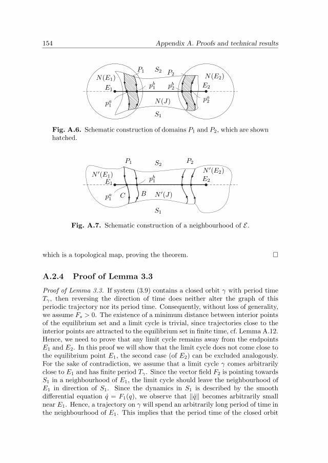
154 Appendix A. Proofs and technical results
N(E1) N(E2)
E1E2
N(J)pa1
pb1 pb
2
pa2
P1 P2
S1
S2
Fig. A.6. Schematic construction of domains P1 and P2, which are shownhatched.
N ′(E1)N ′(E2)
E1E2
N ′(J)pa1
pb1
P1 P2
BC
S1
S2
Fig. A.7. Schematic construction of a neighbourhood of E .
which is a topological map, proving the theorem.
A.2.4 Proof of Lemma 3.3
Proof of Lemma 3.3. If system (3.9) contains a closed orbit γ with period timeTγ , then reversing the direction of time does neither alter the graph of thisperiodic trajectory nor its period time. Consequently, without loss of generality,we assume Fs > 0. The existence of a minimum distance between interior pointsof the equilibrium set and a limit cycle is trivial, since trajectories close to theinterior points are attracted to the equilibrium set in finite time, cf. Lemma A.12.Hence, we need to prove that any limit cycle remains away from the endpointsE1 and E2. In this proof we will show that the limit cycle does not come close tothe equilibrium point E1, the second case (of E2) can be excluded analogously.For the sake of contradiction, we assume that a limit cycle γ comes arbitrarilyclose to E1 and has finite period Tγ . Since the vector field F2 is pointing towardsS1 in a neighbourhood of E1, the limit cycle should leave the neighbourhood ofE1 in direction of S1. Since the dynamics in S1 is described by the smoothdifferential equation q = F1(q), we observe that ‖q‖ becomes arbitrarily smallnear E1. Hence, a trajectory on γ will spend an arbitrarily long period of time inthe neighbourhood of E1. This implies that the period time of the closed orbit

A.2 Appendices of Chapter 3 155
γ becomes arbitrarily long, yielding a contradiction. The lemma is proven.
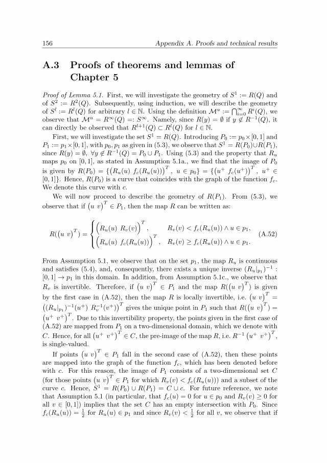
156 Appendix A. Proofs and technical results
A.3 Proofs of theorems and lemmas ofChapter 5
Proof of Lemma 5.1. First, we will investigate the geometry of S1 := R(Q) andof S2 := R2(Q). Subsequently, using induction, we will describe the geometryof Sl := Rl(Q) for arbitrary l ∈ N. Using the definition Mu :=
⋂∞i=0R
i(Q), weobserve that Mu = R∞(Q) =: S∞. Namely, since R(y) = ∅ if y 6∈ R−1(Q), itcan directly be observed that Rl+1(Q) ⊂ Rl(Q) for l ∈ N.
First, we will investigate the set S1 = R(Q). Introducing P0 := p0×[0, 1] andP1 := p1×[0, 1], with p0, p1 as given in (5.3), we observe that S1 = R(P0)∪R(P1),since R(y) = ∅, ∀y 6∈ R−1(Q) = P0 ∪ P1. Using (5.3) and the property that Rumaps p0 on [0, 1], as stated in Assumption 5.1a., we find that the image of P0
is given by R(P0) = (Ru(u) fc(Ru(u))
)T, u ∈ p0 =
(u+ fc(u
+))T, u+ ∈
[0, 1]. Hence, R(P0) is a curve that coincides with the graph of the function fc.We denote this curve with c.
We will now proceed to describe the geometry of R(P1). From (5.3), we
observe that if(u v)T ∈ P1, then the map R can be written as:
R((u v)T
) =
(Ru(u) Rv(v)
)T, Rv(v) < fc(Ru(u)) ∧ u ∈ p1,(
Ru(u) fc(Ru(u)))T
, Rv(v) ≥ fc(Ru(u)) ∧ u ∈ p1.(A.52)
From Assumption 5.1, we observe that on the set p1, the map Ru is continuousand satisfies (5.4), and, consequently, there exists a unique inverse (Ru|p1)−1 :[0, 1]→ p1 in this domain. In addition, from Assumption 5.1c., we observe that
Rv is invertible. Therefore, if(u v)T ∈ P1 and the map R(
(u v)T
) is given
by the first case in (A.52), then the map R is locally invertible, i.e.(u v)T
=((Ru|p1
)−1(u+) R−1v (v+)
)Tgives the unique point in P1 such that R(
(u v)T
) =(u+ v+
)T. Due to this invertibility property, the points given in the first case of
(A.52) are mapped from P1 on a two-dimensional domain, which we denote with
C. Hence, for all(u+ v+
)T ∈ C, the pre-image of the map R, i.e. R−1(u+ v+
)T,
is single-valued.
If points(u v)T ∈ P1 fall in the second case of (A.52), then these points
are mapped into the graph of the function fc, which has been denoted beforewith c. For this reason, the image of P1 consists of a two-dimensional set C
(for those points(u v)T ∈ P1 for which Rv(v) < fc(Ru(u))) and a subset of the
curve c. Hence, S1 = R(P0) ∪ R(P1) = C ∪ c. For future reference, we notethat Assumption 5.1 (in particular, that fc(u) = 0 for u ∈ p0 and Rv(v) ≥ 0 forall v ∈ [0, 1]) implies that the set C has an empty intersection with P0. Sincefc(Ru(u)) = 1
2 for Ru(u) ∈ p1 and since Rv(v) < 12 for all v, we observe that if
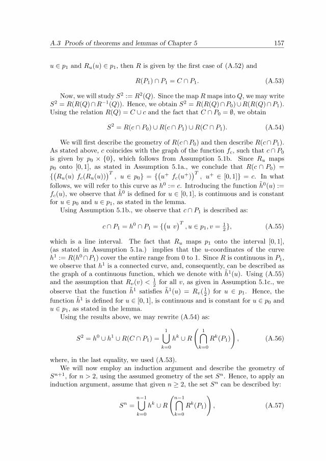
A.3 Proofs of theorems and lemmas of Chapter 5 157
u ∈ p1 and Ru(u) ∈ p1, then R is given by the first case of (A.52) and
R(P1) ∩ P1 = C ∩ P1. (A.53)
Now, we will study S2 := R2(Q). Since the map R maps into Q, we may writeS2 = R(R(Q)∩R−1(Q)). Hence, we obtain S2 = R(R(Q)∩P0)∪R(R(Q)∩P1).Using the relation R(Q) = C ∪ c and the fact that C ∩ P0 = ∅, we obtain
S2 = R(c ∩ P0) ∪R(c ∩ P1) ∪R(C ∩ P1). (A.54)
We will first describe the geometry of R(c∩P0) and then describe R(c∩P1).As stated above, c coincides with the graph of the function fc, such that c ∩ P0
is given by p0 × 0, which follows from Assumption 5.1b. Since Ru mapsp0 onto [0, 1], as stated in Assumption 5.1a., we conclude that R(c ∩ P0) =
(Ru(u) fc(Ru(u))
)T, u ∈ p0 =
(u+ fc(u
+))T, u+ ∈ [0, 1] = c. In what
follows, we will refer to this curve as h0 := c. Introducing the function h0(u) :=fc(u), we observe that h0 is defined for u ∈ [0, 1], is continuous and is constantfor u ∈ p0 and u ∈ p1, as stated in the lemma.
Using Assumption 5.1b., we observe that c ∩ P1 is described as:
c ∩ P1 = h0 ∩ P1 = (u v)T, u ∈ p1, v = 1
2, (A.55)
which is a line interval. The fact that Ru maps p1 onto the interval [0, 1],(as stated in Assumption 5.1a.) implies that the u-coordinates of the curveh1 := R(h0∩P1) cover the entire range from 0 to 1. Since R is continuous in P1,we observe that h1 is a connected curve, and, consequently, can be described asthe graph of a continuous function, which we denote with h1(u). Using (A.55)and the assumption that Rv(v) < 1
2 for all v, as given in Assumption 5.1c., we
observe that the function h1 satisfies h1(u) = Rv(12 ) for u ∈ p1. Hence, the
function h1 is defined for u ∈ [0, 1], is continuous and is constant for u ∈ p0 andu ∈ p1, as stated in the lemma.
Using the results above, we may rewrite (A.54) as:
S2 = h0 ∪ h1 ∪R(C ∩ P1) =
1⋃k=0
hk ∪R(
1⋂k=0
Rk(P1)
), (A.56)
where, in the last equality, we used (A.53).We will now employ an induction argument and describe the geometry of
Sn+1, for n > 2, using the assumed geometry of the set Sn. Hence, to apply aninduction argument, assume that given n ≥ 2, the set Sn can be described by:
Sn =
n−1⋃k=0
hk ∪R(n−1⋂k=0
Rk(P1)
), (A.57)

158 Appendix A. Proofs and technical results
with each curve hk, k = 0, . . . n − 1, given by graphs of a function hk that isdefined for u ∈ [0, 1], is continuous and is constant for u ∈ p0 and u ∈ p1, asstated in the lemma. To employ induction, observe that this assumption implies,using the same arguments as mentioned above, that the set Sn+1 can be writtenas:
Sn+1 =
n⋃k=0
hk ∪R(
n⋂k=0
Rk(P1)
), (A.58)
with the curvehn := R(hn−1 ∩ P1). (A.59)
From the properties of the map R as stated in Assumption 5.1, it directly followsthat the curve hn can be described by the graph of a function hn that is definedfor u ∈ [0, 1], is continuous and is constant for u ∈ p0 and u ∈ p1, as stated inthe lemma.
We can now apply induction, proving that
Sl+1 =
l⋃k=0
hk ∪R(
l⋂k=0
Rk(P1)
),∀l ∈ 2, 3, . . .. (A.60)
Using the fact that Mu = S∞, we obtain:
Mu =
∞⋃k=0
hk ∪R( ∞⋂k=0
Rk(P1)
). (A.61)
Clearly, the set⋃∞k=0 h
k is a union of a countable set of curves. We willnow show that h? := R
(⋂∞k=0R
k(P1))
also is a curve. Assumption 5.1c. states
that the map R is contracting in v-direction for(u, v)∈ P1. Hence, under the
forward iterates of R, the set C will be contracted in v-direction: the widthin v-direction of the set
⋂lk=0R
k(P1) is not larger than λlv, with λv given inAssumption 5.1. Here, we used (A.53) and observed that R(P1)∩P1 is a subsetof the image of the first case in (A.52), such that the size in v-direction ofR(P1) ∩ P1 is at most λv. We can now conclude that
⋂∞k=0R
k(P1) is a curveand, using continuity of R, find that h? = R
(⋂∞k=0R
k(P1))
is a curve. Hence,we observe that Mu = h? ∪⋃∞k=0 h
k, proving the first statement of the lemma.
For all i > 1, hi ⊂ R(⋂i
k=0Rk(P1)
). As mentioned before, the latter set
contracts to the curve h? for i → ∞, such that we observe that the curves hi
converge to the line h? for i→∞.In order to prove that hi ∩hj ∩P1 = ∅ for i, j ∈ N∪?, i 6= j, first, observe
thath0 ∩ hk ∩ P1 = ∅, ∀k ∈ N ∪ ?. (A.62)
since h0∩P1 is given in (A.55), hk∩P1 ⊂ R(P1)∩P1 ⊂ C, for k ∈ N∪?, k 6= 0,(the first and second inclusion follow from (A.59) and (A.53), respectively), and
A.3 Proofs of theorems and lemmas of Chapter 5 159
all v-coordinates of points(u v)T ∈ C satisfy v < 1
2 . Namely, since Rv(v) < 12
for all v ∈ [0, 1], as stated in Assumption 5.1c., the construction of the set C
implies that v < 12 for
(u v)T ∈ C.
Recall that for all(u+ v+
)T ∈ C, the pre-image of the mapR is single-valued,
i.e. R−1(u+ v+
)Tis a singleton. Now, in order to obtain a contradiction, assume
that there exists i, j ∈ N ∪ ?, i, j 6= 0 and i 6= j, and a point y ∈ P1 such thaty ∈ hi ∩ hj ∩ P1. Without loss of generality, assume that i 6= ?, and j > i ifboth i, j ∈ N. Observe that hk ∩ P1 ⊂ C, ∀k ≥ 1, and, consequently, the first iiterates of the inverse map of R, i.e. R−k(y)for k ∈ 0, . . . i, are single-valued.
Using i ∈ N and the definitions of the curves hk, k ∈ N ∪ ?, and theassumption y ∈ hi ∩ P1 which was posed in the previous paragraph, one finds
R−i(y) ⊂ h0 ∩ P1. (A.63)
If j 6= ?, such that j ∈ N, j > i, then the expression y ∈ hj ∩ P1 implies
R−i(y) ⊂ hj−i ∩ P1. (A.64)
A contradiction is now obtained, since the singleton R−i(y) cannot be positionedboth in h0 ∩ P1 and in hj−i ∩ P1, with j − i > 0, since these sets have anempty intersection according to (A.62). If j = ?, then y ∈ h? ∩ P1 impliesR−i(y) ∈ h? ∩P1, since, from continuity of R and the definition of h?, it followsthat h? = R(h?∩P1). Again, the singleton R−i(y) cannot simultaneously satisfyR−i(y) ∈ h? ∩ P1 and R−i(y) ∈ h0 ∩ P1 due to (A.62).
Hence, for both j ∈ N, j > i and for j = ?, a contradiction is obtained, suchthat hi ∩ hj ∩ P1 = ∅ when i, j ∈ N ∪ ?, i, j 6= 0, and i 6= j. From (A.62),we observe that we can select i = 0 in this expression as well, such that thestatement hi ∩ hj ∩ P1 = ∅ for i, j ∈ N ∪ ?, i 6= j, as presented in the lemma,is obtained.
The last statement of the lemma follows directly from the construction ofthe curves hi, i ∈ N, as given in (A.59), such that the lemma is proven.
Proof of Theorem 5.2. First, we prove that τ : X → Sc is surjective and continu-ous. Subsequently, we will prove invertibility of τ , and continuity of its inverse.Finally, we show σc(τ(y)) = τ(R|X (y)), such that the map τ is a topologicalconjugacy as in Definition 5.3, with Φ = R|X and Ψ = σc.Surjectiveness of τTo prove that τ is surjective, we prove that for each a ∈ Sc there exists an y ∈ Xsuch that a = τ(y).
First, we will show that given any a ∈ Sc, there exists a u ∈ [0, 1] such that
for appropriate v, the points τ((u v)T
) ∈ Sc and a ∈ Sc have identical elements
τ((u v)T
)i = ai for i ∈ N. For i ≥ 0, from (5.16), we conclude that τ((u v)T
)i
is determined by the u-coordinate of Ri((u v)T
). From (5.3), we observe that

160 Appendix A. Proofs and technical results
these points are described by the iterates of the map Ru. By construction of
the sets P0, P1, a point Ri((u v)T
), for i ≥ 0, satisfies Ri((u v)T
) ∈ P0, or
Ri((u v)T
) ∈ P1 if and only if Riu(u) ∈ p0 or Riu(u) ∈ p1, respectively.By Assumption 5.1a., the map Ru maps both p0 and p1 onto [0, 1]. Con-
sequently,R−1u (pi) ∩ pj 6= ∅, for i, j ∈ 0, 1. (A.65)
We observe that in two iterates, the set R−1u (pi)∩pj is mapped onto the complete
line interval [0, 1]. Using this property iteratively, given a point a ∈ Sc, weobserve that the set sj(a) defined by
sj(a) :=
j⋂m=0
R−1u (pam), j ∈ N (A.66)
is nonempty for every finite j. In addition, the iterates of the map Ru will satisfyRmu (u) ∈ pam for all m ∈ 0, . . . j if u ∈ sj(a).
Observe that sj(a)j∈N is a sequence of nested nonempty closed intervals onR, and for this reason, s∞(a) := limj→∞ sj(a) is nonempty and closed, as stated
in the nested sphere theorem in [93, p60]. Hence, given any point(u v)T ∈ X
with u ∈ s∞(a), we observe that Ri((u v)T
) ∈ Pai , ∀i ≥ 0. Consequently,
τ((u v)T
)i = ai, ∀i ≥ 0, cf. (5.16).
Now, given a ∈ Sc, we will select v such that τ((u, v)) = a if u ∈ s∞(a).
For this purpose, let k ∈ N ∪ ? either be the maximum integer such thatai = 1, i ∈ [−k,−1], or be given by k = ? if ai = 1, ∀i ∈ (−∞,−1]. Let
v = hk(u), with hk as defined in Lemma 5.1. Then(u v)T ∈ X is such that
a = τ((u v)T
). Since a ∈ Sc was taken arbitrarily, τ : X → Sc is surjective.Continuity of τ
To prove continuity of τ in (5.16), we show that for all ε > 0 there exists a δ > 0such that for all y0, y1 ∈ X with ‖y0 − y1‖ < δ, ρc(τ(y0), τ(y1)) < ε, with ρc asin Definition 5.2. For this purpose, we first select an integer ¯≥ 1 satisfying
¯> − log2(ε), (A.67)
and observe that if the distance ρc(τ(y0), τ(y1)) is evaluated and `, as givenin Definition 5.2, can be chosen to satisfy ` ≥ ¯, then ρc(τ(y0), τ(y1)) < εis obtained. Hence, we will prove continuity of τ by proving that given anarbitrarily large integer ` ≥ 1, we can select δ > 0 such that ¯ ≤ ` in theevaluation of ρc(τ(y0), τ(y1)).
Note that ‖y0 − y1‖ < δ implies |u0 − u1| < δ if we use the notation yi =(ui vi
)T, i = 0, 1. Let G = inf u0∈p0,u1∈p1
|u0 − u1| be the minimum distance
between p0 and p1. If we select δ < λ−¯G, with λ given in Assumption 5.1a.,
then, using the same assumption, we conclude that |Riu(u0)−Riu(u1)| ≤ λ¯δ < G,

A.3 Proofs of theorems and lemmas of Chapter 5 161
for all i ∈ [0, ¯], which, by the design of G, implies that for each i ∈ [0, ¯], Riu(u0)and Riu(u1) lie in the same set p0 or p1. Since the u-coordinates of the map R,as given in (5.3), are described by the iterates of the map Ru, we conclude thatRi(y0) and Ri(y1) lie in the same set P0 or P1 for each i ∈ [0, ¯]. Hence, (5.16)implies (τ(y0))i = (τ(y1))i for i ∈ [0, ¯].
First consider the case (τ(y0))0 = (τ(y1))0 = 0 and afterwards, the case(τ(y0))0 = (τ(y1))0 = 1.
If (τ(y0))0 = (τ(y1))0 = 0, then, in the evaluation of ρc(τ(y0), τ(y1)) as givenin Definition 5.2, we can set k = 0, such that the conclusion of the previousparagraph directly implies that `, as given in Definition 5.2, can be chosenlarger than, or equal to ¯. Hence, ρc(τ(y0), τ(y1)) = 2−` ≤ 2−
¯. From (A.67),
we conclude 2−¯< ε, such that we obtain ρc(τ(y0), τ(y1)) < ε.
If (τ(y0))0 = (τ(y1))0 = 1, then the distance ρc(τ(y0), τ(y1)) also dependson the v-coordinates of the points y0 and y1, since (τ(y0))0 = (τ(y1))0 = 1imply y0, y1 ∈ P1. The integers κ(y0) and κ(y1) as given the theorem may bedifferent, since all curves hi, i ∈ N ∪ ?, have a nonempty intersection withP1, and, consequently, both points y1 and y2 can be positioned in any curvehi, i ∈ N ∪ ?.
Given any finite integer ¯ > 0, there exists a δ¯ > 0 such that for eachi ∈ [0, ¯], the curve hi ∩ P1 is more than the distance δ¯ away from all the othercurves hj , with i, j ∈ N ∪ ?, j 6= i, i.e.
P1 ∩ hi + Bδ¯ ∩ hj = ∅, ∀j ∈ (N ∪ ?) \ i, for each i ∈ [0, ¯]. (A.68)
Here, we used the facts that for each finite i ≥ 0, both the curve hi and theset y ∈ Q,∃j ∈ (N ∪ ?) \ i, y ∈ hj are closed, and hi ∩ hj ∩ P1 = ∅for i 6= j, i, j ∈ N ∪ ?, as stated in Lemma 5.1. From (A.68), we concludethat, if y0, y1 ∈ P1 ∩ X and |y0 − y1| < δ¯, then either y0 and y1 are positionedin the same curve hi, i ∈ [0, ¯] (such that κ(y0) = κ(y1)), or y0 ∈ hk0 andy1 ∈ hk1 , with k0, k1 ∈ [¯+ 1,∞). In both cases, from (5.16), we conclude that(τ(y0))i = (τ(y1))i for i ∈ [max(−¯,−κ(y0)),−1].
Consequently, if δ > 0 is chosen smaller than min(δ¯, λ−¯G), then we have ob-
tained (τ(y0))i=(τ(y1))i for i ∈ [max(−¯,−κ(y0)), ¯]. We find ρc(τ(y0), τ(y1))<ε, proving continuity of τ .
Invertibility of τTo prove invertibility of τ , assume that there exists an a ∈ Sc and two distinct
points y0, y1 ∈ X such that τ(y0) = τ(y1) = a. Let yi =(ui vi
)T, i = 0, 1. First,
we will show that u0 = u1 if τ(y0) = τ(y1) = a. Using the same constructionas above, let the intervals si(a), i ∈ N, denote the u-coordinates of the initialconditions in Q whose trajectories visit the sequence a0 . . . ai of domains P0 andP1 in the next i iterates of the map R, such that s0(a) = pa0 and si+1(a) = u ∈si(a), Ri+1
u (u) ∈ pai+1. From Assumption 5.1a. and the definition of si(a), for

162 Appendix A. Proofs and technical results
i ∈ N and a ∈ Sc, given in (A.66), we observe that
supu0,u1∈si(a)
|u0 − u1| ≤ λ−i,∀i ≥ 0, with λ > 1. (A.69)
Since τ(y0) = τ(y1), the symbols τ(y0)i and τ(y1)i coincide for all i ≥ 0, whichimplies that u0, u1 ∈ si(a),∀i. Hence, with (A.69), we obtain u0 = u1.
To study the v-coordinates of the points y0 and y1, observe that the defin-itions of τ and κ in the theorem imply that κ(y0) and κ(y1) have to be equalwhen τ(y0) = τ(y1), and hence, the v-coordinate of both y0 and y1 are given,for finite κ(y0), by hκ(y0)(u0), and, for κ(y0) =∞, by h?(u0), with the functionshi, i ∈ N∩ ?, given in Lemma 5.1. Hence, we obtained v0 = v1. Combinationof this result with the conclusion of the previous paragraph, yields the conclu-sion that y1 = y0, which contradicts distinctness of y0 and y1. A contradiction isobtained, such that for any two distinct points y0, y1 ∈ X , τ(y0) 6= τ(y1) holds.Hence, τ is invertible.
Continuity of τ−1
Now, we will prove that τ−1 is continuous by showing that for all ε > 0 thereexists a δ > 0 such that for a, b ∈ Sc, ρc(a, b) < δ implies
|τ−1(a)− τ−1(b)| < ε. (A.70)
In fact, we will prove the stronger requirement that both
|πu(τ−1(a))− πu(τ−1(b))| <√
22 ε, (A.71)
and|πv(τ−1(a))− πv(τ−1(b))| <
√2
2 ε, (A.72)
hold when πu(y) and πv(y) denote the u-, or v-coordinates of points y ∈ X ,respectively.
Given two points a, b ∈ Sc, let k be as given in Definition 5.2 for the evaluationof ρc(a, b). We will prove continuity of τ−1 by showing that, if we select abounded L satisfying
L >− log
(√2
2 ε)
log(λ), (A.73)
and, in addition,ai = bi, ∀i ∈ [max(−L,−k), L] (A.74)
holds, then (A.71) and (A.72) are satisfied. We note that for any bounded L,(A.74) will be satisfied when δ > 0 is chosen sufficiently small and ρc(a, b) < δis satisfied.
Given ai = bi, ∀i ∈ [0, L], we observe that for each i ∈ [0, L], Ri(τ−1(a)) andRi(τ−1(b)) are in the same set P0 or P1. Hence, πu(τ−1(a)) and πu(τ−1(b)) arecontained in the same set sL(a), with the interval sL(a) as constructed above.

A.3 Proofs of theorems and lemmas of Chapter 5 163
Combination of (A.69), (A.73) and πu(τ−1(a)), πu(τ−1(b)) ∈ sL(a) proves that(A.71) is satisfied.
Now, we will prove for each ε > 0, there exists a finite Lε > 0 such that ifL > Lε, then (A.74) implies (A.72).
If max(−L,−k) = −k, then k is finite, κ(τ−1(a)) = κ(τ−1(b)) = k, with thefunctions κ as given in the theorem, and τ−1(a), τ−1(b) ∈ hk. From L ≥ 1, weconclude that either both τ−1(a) ∈ P0 and τ−1(b) ∈ P0, or τ−1(a), τ−1(b) ∈ P1
hold. Hence, combination of the observations that πv(τ−1(a)) = hk(πu(τ−1(a))),
πv(τ−1(b)) = hk(πu(τ−1(b))) and that every function hk(u), k ∈ N ∪ ∞,
is constant for u ∈ p0 or u ∈ p1 leads to the conclusion that πv(τ−1(a)) =
πv(τ−1(b)), such that (A.72) is satisfied when k ≤ L is finite.
It remains to be proven that one can select Lε > 0 such that (A.72) is satisfiedwhen L > k and L > Lε. Again, we use the fact that L > 0, such that bothτ−1(a) and τ−1(b) are positioned in the same set P1 or P0.
Since the curves hi converge to h? when i is increased to infinity, and, inaddition, the functions hi(u), i ∈ N ∪ ?, are constant on the intervals u ∈p0 and u ∈ p1, we observe that we can select a finite integer Lε such that
|hi(u0) − hj(u1)| <√
22 ε for all i, j ∈ k ∈ N, k ≥ Lε ∪ ?, when u0 and
u1 are positioned in the same interval p0 or p1. In addition, we note thatL > Lε, (A.74) and (5.16) together imply τ−1(a) ∈ hka and τ−1(b) ∈ hkb withka, kb ∈ k ∈ N, k ≥ Lε ∪ ?. Hence, we obtain
|πv(τ−1(a))−πv(τ−1(b))| = |hka(πu(τ−1(a)))−hkb(πu(τ−1(b)))| <√
22 ε. (A.75)
We can now conclude that if L > max(Lε,− log(
√2ε)
log(λ) ), then both (A.71) and
(A.72) are guaranteed to hold, such that (A.70) is satisfied. Hence, if δ = 2−L
holds, then |τ−1(a) − τ−1(b)| < ε is guaranteed when ρc(a, b) < δ, such thatcontinuity of τ−1 is proven.
ConjugacyWe have now proven that the function τ is a homeomorphism. It remains tobe proven that σc(τ(y)) ∼ τ(R(y)). Let κ(y) be as given in the theorem andobserve that (5.16) implies
(σc(τ(y)))i = τ(y)i+1 =
0, i ∈ (−∞,−κ(y)− 2],1, i ∈ [−κ(y)− 1,−2],0, i ∈ [−1,∞) ∧Ri+1(y) ∈ P0,1, i ∈ [−1,∞) ∧Ri+1(y) ∈ P1.
(A.76)
To show that this expression coincides with τ(R(y))i, i ∈ Z, we distinguish threecases, namely, R(y) ∈ P0, R(y) ∈ P1 ∩ h0 and R(y) ∈ P1 ∩
(h? ∪⋃∞i=1 h
i).
In the first case, i.e. the case where R(y) ∈ P0, from hi ∩ P0 = hj ∩ P0, ∀i, j,as stated in Lemma 5.1, we conclude that κ(R(y)) = 0. Hence, the definition of
164 Appendix A. Proofs and technical results
τ given in (5.16) gives, for κ(R(y)) = 0,
τ(R(y))i =
0, i ∈ (−∞,−1],0, i ∈ [0,∞) ∧Ri+1(y) ∈ P0,1, i ∈ [0,∞) ∧Ri+1(y) ∈ P1,
(A.77)
which coincides with (A.76), since we observe τ(R(y))0 = (σc(τ(y)))0 = 0 asR(y) ∈ P0, and τ(R(y))i = (σc(τ(y)))i,∀i ∈ [1,∞), which, using Definition 5.1,directly imply τ(R(y)) ∼ σc(τ(y)).
In the second case, i.e. where R(y) ∈ P1 ∩ h0, we observe that κ(R(y)) =0. Hence, again, τ(R(y)) is given by (A.77). Note that (A.76) and (A.77)clearly coincide for all indices i 6= −1. To evaluate (A.76) for i = −1, observethat R(y) ∈ h0 ∩ P1, can only hold when y ∈ P0, such that (τ(y))0 = 0, andtherefore, (σc(τ(y)))−1 = 0. Hence, (A.77) and (A.76) coincide for all i, suchthat τ(R(y)) ∼ σc(τ(y)).
The last case to be considered is R(y) ∈ P1 ∩(h? ∪⋃∞i=1 h
i). Since κ(y),
for y ∈ X , denotes the minimum integer such that y ∈ hκ(y) if κ(y) is finite,and y ∈ h? if κ(y) = ∞, we conclude that κ(R(y)) ∈ k ∈ N, n ≥ 1 ∪ ∞.It can be observed, for the case where κ(y) is finite, that the last statement ofLemma 5.1 implies κ(R(y)) = κ(y) + 1. Hence, we find
τ(R(y))i =
0, i ∈ (−∞,−κ(R(y))− 1] = (−∞,−κ(y)− 2],1, i ∈ [−κ(R(y)),−1] = [−κ(y)− 1,−1],0, i ∈ [0,∞) ∧Ri+1(y) ∈ P0,1, i ∈ [0,∞) ∧Ri+1(y) ∈ P1,
(A.78)
which clearly coincides with (A.76) for all i 6= −1. To see that (A.76) and(A.78) also coincide for i = −1, we note that R(y) ∈ hκ(R(y)) implies y ∈hκ(R(y))−1 ∩ P1, cf. the last statement of Lemma 5.1. Hence, (A.76) impliesσc(τ(y))−1 = (τ(y))0 = 1, and, consequently, σc(τ(y))i = τ(R(y))i, ∀i ∈ Z.
From (5.8) and Lemma 5.1, we conclude that each R(y) ∈ X falls in one ofthe cases described above. Therefore, we have proven that the diagram
XR|X //
τ
Xτ
Sc σc
// Sc
commutes. Hence, the homeomorphism τ is a topological conjugacy betweenthe dynamical systems (X , R|X ) and (Sc, σc), which concludes the proof of thetheorem.
Proof of Lemma 5.4. Topological transitivity is invariant under topological con-jugacies, cf. [110, p. 198], such that we will prove the equivalent statement that

A.3 Proofs of theorems and lemmas of Chapter 5 165
(Sc, σc) is topologically transitive. For this reason, using the approach givenin [92], a point a ∈ Sc is constructed whose orbit under σc is dense in Sc.
Let εii∈N be a sequence of strictly positive numbers monotonically conver-ging to zero. First, for each εi > 0, we will construct a finite block of symbolsai = ai0a
i1 . . . a
ini such that any trajectory of σc from a point b ∈ Sc, where b
starts with the block ai, comes in an εi-neighbourhood of each point r ∈ Sc.By concatenating these blocks ai, as we will show below, we will find a pointa = (. . . 1.a0a1a2 . . .) ∈ Sc whose orbit is dense in Sc.
Namely, the orbit from the point a under the shift map is dense if for eachδ > 0 and any point p ∈ Sc, we can find a time T such that ρc(σ
Tc (a), p) < δ. If
the point a is constructed as above, then, given δ, we can select a finite i > 0such that εi < δ. Since the point a contains the block ai in its future elements,the orbit from a will arrive in every εi-neighbourhood in Sc, and, consequently,also in an εi-neighbourhood of the point p.
We will now proceed to construct the blocks ai with the properties givenabove. Given εi > 0, observe that for each r ∈ Sc, q ∈ Sc, ρc(r, q) < εi,consists of points q with ri = qi for i ∈ [max(−`i,−k), `i], where k is thenonnegative integer as defined in Definition 5.2, and `i is the minimum numbersuch that 2−`
i
< εi. Let r[−`i,`i] denote the block r−`ir−`i+1 . . . r`i .Since each element ri, i ∈ [−`i, `i] of a point r satisfies ri ∈ 0, 1, which
contains two elements, we can select a finite number ni ≤ 22`i+1 of different
points rj such that Sc =⋃nij=1q ∈ Sc, ρc(rj , q) < εi. Hence, we can construct
the block ai, which has finite length, by concatenation of the blocks rj[−`i,`i],
such that ai = r0[−`i,`i]r
1[−`i,`i] . . . r
ni
[−`i,`i]. Any trajectory of σc of a point b ∈ Scthat contain the block ai in the sequence bi, i ∈ N, becomes εi-close to everypoint in Sc, as this trajectory visits every εi-neighbourhood in Sc. Namely, forevery j ∈ 1, . . . ni, after a finite number κ of iterations, (σκc (b))[−`i,`i] = rj[−`i,`i]holds.
By concatenating these blocks ai for i ∈ N, we obtain a point a ∈ Sc givenby a = . . . 1.a0a1a2 . . ., whose orbit is dense in Sc. Hence, from Definition 5.4,we conclude that the dynamical system (Sc, σc) is transitive. Since (X , R|X )is topologically conjugate to this system, (X , R|X ) is topologically transitive aswell, proving the lemma.

166 Appendix A. Proofs and technical results
A.4 Local phase portrait near an equilibrium setof a periodically forced mechanical systemwith dry friction
In this section, we describe the local phase portrait near a periodically forcedmechanical system with dry friction, which has been discussed briefly in Chap-ter 4. In this section, we aim to describe this local phase portrait in more detail.
As mentioned in Remark 5.2, we expect that the return maps as describedin Chapter 4 form a subset of the class of discrete-time systems described inSection 5.2. This statement would lead to the conclusion that horseshoe-typelimit sets of the nature presented in Chapter 5 can exist in periodically forcedmechanical systems with dry friction. We provide the results in this appendixsince we expect that this will form a first step in a proof of such a statement,which will further motivate the work in Chapter 5.
Throughout this section, we consider models of mechanical systems with onedegree of freedom that experience dry friction, modelled with an Amontons-Coulomb friction element. In appropriate coordinates, these systems can bedescribed by the following differential inclusion:
x ∈ f(x, x)− Fs Sign(x) + εg(t), (A.79)
where x ∈ R, and solutions are considered in the sense of Filippov, cf. [58]. Inthe differential inclusion (A.79), the set-valued sign function
Sign(x) =
x|x| , x 6= 0
[−1, 1], x = 0,(A.80)
is used, such that the dry friction force is contained in the set Fs Sign(x), whereFs > 0. Other forces acting on the system, that can include gravitational forces,damping forces and forces due to flexibilities, are described by the force f(x, x).We assume that f(x, x) is a smooth function. Time-dependent forces, e.g. per-turbations or actuation forces, are modelled with the term εg(t), with |g(t)| ≤ 1for all t. Throughout this appendix, we assume that εg(t) is a periodic functionof time and that ε is small.
In the next section, we will apply some results presented in Chapter 3 to thesystem (A.79) when the perturbation is absent, i.e. when ε = 0.
A.4.1 Unperturbed system dynamics
We consider (A.79) as a periodically perturbed version of an autonomous differ-ential inclusion with ε = 0, given by:
x ∈ f(x, x)− Fs Sign(x). (A.81)
A.4 Local phase portrait near an equilibrium set with periodic forcing 167
We describe the phase portrait of this differential inclusion using the results ofChapter 3. In that chapter, we show that the phase space of system (A.81)contains equilibrium sets, i.e., line intervals consisting of non-isolated equilibria,
and these line-shaped equilibrium sets are given by the points(x x)T ∈ R2,
where f(x, 0) ∈ Fs Sign(0) and x = 0. Trajectories can converge in finite timeto points in the equilibrium set, whereas asymptotic convergence (i.e. trajector-ies that approach the equilibrium set with an infinitely long transient time) orasymptotic divergence (i.e. trajectories that, after reversing the direction of time,show asymptotic convergence) can only occur at the endpoints of the equilibriumset.
To analyse the phase portrait of the autonomous system (A.81), we introducethe following first-order Filippov system:
y ∈ aF (y) :=
(y2
f(y1, y2)− Fs Sign(y2)
), (A.82)
which is equivalent to (A.81) when selecting y =(y1 y2
)T:=(x x)T ∈ R2. The
discontinuity of (A.82) is restricted to a single surface:
aΣ := y ∈ R2, y2 = 0. (A.83)
We observe that away from the discontinuity, the function aF in (A.82) satisfies
aF (y) = aF+(y) :=
(y2
f(y1, y2)− Fs
), for y2 > 0
aF (y) = aF−(y) :=
(y2
f(y1, y2) + Fs
), for y2 < 0,
(A.84)
where aF+ and aF− are smooth functions. Using the approach of Filippov tostudy solutions to differential inclusions, cf. [58], we distinguish two subsets ofaΣ in (A.83), denoted by aΣc and aΣs, where aF+ and aF− allow the trajectoriesof (A.82) to cross aΣ instantaneously, or where this is not possible, respectively.According to [58], these sets can be given as:
aΣc := y ∈ aΣ, aF+2(y) aF−2(y) > 0, (A.85)aΣs := y ∈ aΣ, aF+2(y) aF−2(y) ≤ 0, (A.86)
where aF+2(y) and aF−2(y) denote the second component of aF+(y) and aF−(y),respectively. If a trajectory φ of (A.82) arrives in aΣc, that is, if for a givent, φ(t) ∈ aΣc, then this trajectory can be continued by selecting either y =aF+(y) (when aF+2(ϕ(t)) > 0) or y = aF−(y) (when aF−2(ϕ(t)) < 0). If, fora given time t, φ(t) ∈ aΣs holds, then neither y = aF+(y) nor y = aF−(y)can be used to continue the solution from this point. Consequently, Filippov’ssolutions concept requires such solutions to stay at the surface aΣ, such that thedifferential equation dφ
dt = 0 holds almost everywhere for φ(t) ∈ aΣs. Hence, the

168 Appendix A. Proofs and technical results
set aΣs coincides with a set of equilibrium points, and we introduce E0 := aΣs
to refer to this equilibrium set.In order to describe the effect of a small time-periodic perturbation on the
stick set aΣs and aΣc, we impose the following assumption on the differentialinclusion (A.79).
Assumption A.1. Consider system (A.79) and let, for the autonomous case
ε = 0, E0 =(Ex0 0
)Tdenote the y-coordinates of an endpoint of an equilibrium
set where aF− vanishes, i.e. where aF−(E0) = 0. In addition, the smooth func-
tion f satisfies ∂f(x,0)∂x
∣∣∣Ex0
> 0. Assume that the function g(t) is smooth and
periodic with minimal period T > 0.
As mentioned before, the analysis of system (A.79) is motivated by the ana-lysis of a transversal homoclinic orbit emanating from the endpoint of an equi-librium set. We expect such homoclinic orbits to be present for small ε > 0when the autonomous system (A.82) has a single homoclinic orbit from the end-point E0, and, consequently, contains trajectories that leave the neighbourhoodof the point E0 and emanate away from the equilibrium set. This motivates the
assumption that ∂f(x,0)∂x
∣∣∣Ex0
is positive in Assumption A.1, such that trajectories
of (A.82) may cross Σc at x-values slightly below Ex0 from the domain where xis positive to the domain where x is negative. Subsequently, since x is negative,such trajectories leave the neighbourhood of the point E0.
In the following section, we study the effect of a small time-periodic perturb-ation of the system (A.82) on the trajectories near the point E0. In fact, sucha perturbation creates a complex geometrical structure of trajectories conver-ging to, or diverging from the endpoint of the equilibrium set, similar to thehomoclinic tangle in smooth differential equations.
A.4.2 Effect of a time-dependent perturbation
Now, we will consider the phase portrait of the system (A.79) for small ε 6= 0,which can be considered as a small perturbation of the dynamics of (A.81). Forthis purpose, firstly, we introduce an autonomous system representing the dy-namics of (A.79) by embedding the time as an additional state. Subsequently,near the point E0 given in Assumption A.1, we describe the geometrical proper-ties of the two sets where Filippov solutions can cross or stick to the discontinuitysurface, respectively, and note that equilibrium points are given by trajectoriesthat stick to the discontinuity for all time. Hence, the geometrical descriptionof the stick-set and crossing-set will yield a description of the equilibrium set of(A.79) as an additional result. This analysis will be made in Section A.4.2.1.Subsequently, in Section A.4.2.2, we will describe the trajectories that convergeto, or diverge from the boundary of this equilibrium set, and, in this manner, ob-tain a non-smooth analogue of the stable and unstable manifolds of isolated equi-
A.4 Local phase portrait near an equilibrium set with periodic forcing 169
librium points in smooth systems. This information is used in Section A.4.2.3 todescribe the local phase portrait near the endpoint E0 given in Assumption A.1.
We reformulate the dynamics of (A.79) as an autonomous first-order differ-ential inclusion by embedding time as an additional state, yielding state vector
q =(t x x
)T ∈ R3. In this manner, the dynamics of (A.79) is represented by
q ∈ F (q) :=
1q3
f(q2, q3)− Fs Sign(q3) + εg(q1)
. (A.87)
Let S(q0) denote the set of solutions ϕ with initial condition q0, such that allϕ ∈ S(q0) satisfy (A.87) and ϕ(0) = q0. Now, let
Σ := q ∈ R3, q3 = 0, (A.88)
denote the surface where F (q) in (A.87) is discontinuous. Trajectories can crossΣ instantaneously on
Σc := q ∈ Σ, (f(q2, q3)− Fs + εg(q1)) (f(q2, q3) + Fs + εg(q1)) > 0, (A.89)
and sliding motion in the sense of Filippov occurs at the surface
Σs := q ∈ Σ, (f(q2, q3)− Fs + εg(q1)) (f(q2, q3) + Fs + εg(q1)) ≤ 0. (A.90)
The sliding motion of (A.87) is parallel to Σ, cf. [58], and, since in addition
q2 = q3 = 0 at this surface, the sliding motion is described by q =(1 0 0
)Tfor
almost all t. Hence, we conclude that trajectories of (A.87) satisfy:
q =
F+(q) :=
1
q3
f(q2, q3)− Fs + εg(q1)
, q ∈ D+ := q ∈ R, q3 > 0,
F−(q) :=
1
q3
f(q2, q3) + Fs + εg(q1)
, q ∈ D− := q ∈ R, q3 < 0,
F0(q) :=
1
0
0
, q ∈ Σs,
(A.91)for almost all t.
A.4.2.1 Description of the dynamics at the discontinuity surface
Note, that for ε = 0, the boundary between Σc and Σs is given by one or morestraight lines. One of these lines is given by R × E0, which represents the

170 Appendix A. Proofs and technical results
Fig. A.8. Pictorial of the sets Σs and Σc for system (A.87). (a) for ε = 0.(b) for ε > 0.
equilibrium point E0 of (A.82) as a line in the phase space of system (A.87),as depicted in Fig. A.8(a). For small ε > 0, we expect that the boundariesbetween Σc and Σs, given by lines for ε = 0, persist and deform to curves in thephase space of (A.87) due to the small term εg(q1), as depicted in panel (b) ofFig. A.8. The following lemma describes the curve from this set that convergesto R× E0 for ε→ 0.
Lemma A.17. Suppose that Assumption A.1 is satisfied by system (A.79) with
endpoint E0 =(Ex0 0
)T. Let T denote the minimal period of g.
For any δ > 0 we can find an upper bound ε such that for each ε ∈ (0, ε]there exists a function cp : R → [Ex0 − δ, Ex0 + δ] with the following property.Locally near R × E0, the boundary between Σc and Σs, as defined in (A.89)and (A.90), respectively, is given by
c := q ∈ R3, q =(q1 cp(q1) 0
), q1 ∈ R, (A.92)
and the function cp is continuously differentiable and periodic with minimalperiod T .
Proof. According to Assumption A.1, the endpoint E0 =(Ex0 0
)Tof (A.82)
satisfies aF−(E0) = 0, such that
f(Ex0 , 0) + Fs = 0. (A.93)
Consequently, for sufficiently small ε > 0, the definition of Σc and Σs in(A.89)-(A.90) implies that the boundary between Σs and Σc near R × E0 isgiven by the points q ∈ Σ such that F−3(q) = 0, where F−3 denotes the thirdcomponent of F− defined in (A.91). With (A.91), this implies that the expression
f(q2, 0) + Fs = −εg(q1) (A.94)
A.4 Local phase portrait near an equilibrium set with periodic forcing 171
defines the boundary between Σs and Σc near R× E0.
By Assumption A.1, ∂f(x,0)∂x
∣∣∣x=Ex0
6= 0, such that application of the inverse
function theorem to (A.93) implies that there exists an diffeomorphism α(γ)such that α(0) = Ex0 and
f(α(γ), 0) + Fs = −γ (A.95)
holds for all γ in a neighbourhood U of zero. We now select ε > 0 small enoughsuch that εg(q1) ∈ U ∀q1, ε ∈ (0, ε].
Now, given a parameter ε ∈ (0, ε], we define the continuously differentiablefunction
cp(q1) := α(εg(q1)), (A.96)
such that for all q ∈ c, with c defined in (A.92), the expression (A.94) is satisfied.As observed, (A.94) locally characterises the boundary between Σs and Σc, suchthat the curve c defined in (A.92) gives the boundary between Σc and Σs nearR × E0. Since g is periodic with minimal period T , the function cp(q1) isperiodic with the same period, proving the lemma.
The curve c given in (A.92) is depicted schematically in Fig. A.8(b). On the
set Σs, solutions of (A.87) satisfy the Filippov solution q =(1 0 0
)T. Recall
that the first element of the state vector q was added to represent the timet, such that trajectories of (A.87) that remain in Σs for all t correspond toequilibrium positions of (A.79). These trajectories are located in the set Eε :=
q ∈ R3, q +(t 0 0
)T ∈ Σs, ∀t ∈ R, as depicted in Fig. A.8(b). Observethat near R × E0, the set Eε ⊂ Σ is bounded by the line Eε := R × Eε, with
Eε =(maxq∈c q2 0
)Tand c given by (A.92). Trajectories on the set Σs \ Eε will
only stick temporarily to the surface Σ, and, subsequently, will leave this set.The set Eε is the equilibrium set of the system (A.87), consisting of trajectoriesthat stick permanently.
In the next section, we will describe the local dynamics near the equilibriumpositions Eε, by the introduction of the stable and unstable sets of trajectoriesconverging to Eε in forward or backward direction of time, respectively. Insmooth systems with hyperbolic equilibrium points with a saddle-type nature,the existence of a local coordinate system where the flow of (A.79) is contractingin one direction and expanding in the other can be obtained using an hyperbolicsplitting of the phase space, cf. [145]. This result is not applicable in our case dueto the discontinuity of (A.87). However, as we will show in the next section, theunstable set consists of a two-dimensional set where the dynamics is expandingaway from the equilibrium position Eε, and the stable set constitutes of a two-dimensional set in the phase space that contains trajectories that are contractedtowards this equilibrium position. We note, however, that we can not concludefrom the contracting and expanding characteristics of these two sets that, in the
172 Appendix A. Proofs and technical results
rest of the neighbourhood of Eε, the vector field is contracting in one direction,and expanding in the other.
A.4.2.2 Local stable and unstable sets of the endpoint of the equi-librium set
In order to study the local phase portrait near Eε (a boundary of the equilibriumset Eε of (A.87)), we focus on trajectories converging to, or diverging from, Eε.In this manner, we identify two sets in the phase space that play the same role asstable and unstable manifolds of isolated equilibrium points in smooth systems.In this section, we will describe the local dynamical behaviour on these sets.Afterwards, we will use this description in Section A.4.2.3 to analyse the localdynamical behaviour near Eε.
We consider the sets:
Ms := q0 ∈ R3, ∀ϕ ∈ S(q0), limt→∞
d(ϕ(t),Eε) = 0, (A.97a)
Mu := q0 ∈ R3, ∃ϕ ∈ S(q0), limt→−∞
d(ϕ(t),Eε) = 0, (A.97b)
where we recall that S(q0) denotes the set of solutions ϕ of (A.87) from initialcondition ϕ(0) = q0. We will refer to Ms and Mu as the stable and unstable setof Eε, respectively. The asymmetry in the definitions of Ms and Mu stems fromthe fact that trajectories of (A.87) are uniquely defined in forward time, but canbe non-unique in backward time. Note that a stroboscopic projection of thesesets coincide with the stable and unstable sets defined in [73].
Remark A.1. The definition in (A.97) directly implies that Ms is invariant (bothin forward and backward direction of time) under the dynamics (A.87). However,the set Mu is only forward invariant, but not backward invariant under thesedynamics. C
In the neighbourhood of Eε, the set Ms (or Mu) may contain initial conditionsof trajectories that leave the neighbourhood of Eε before converging to Eε underthe flow of (A.87) in forward (or backward) direction of time. Consequently,analogously to the definition of local stable and unstable manifolds in smoothsystems, cf. [142], we define the local stable and unstable sets of Eε as:
Msβ := q0 ∈ R3,∀ϕ ∈ S(q0), lim
t→∞d(ϕ(t),Eε) = 0 and d(ϕ(t),Eε) ≤ β, ∀t ≥ 0,
(A.98a)
Muβ := q0 ∈ R3,∃ϕ ∈ S(q0), lim
t→−∞d(ϕ(t),Eε) = 0 and d(ϕ(t),Eε) ≤ β, ∀t ≤ 0,
(A.98b)
where β > 0 is small.We will now derive two results (Lemma A.18 and Lemma A.19) for the
trajectories in the local stable and unstable sets.
A.4 Local phase portrait near an equilibrium set with periodic forcing 173
The trajectories in Msβ satisfy a finite-time convergence property, as formal-
ised in the following lemma.
Lemma A.18. Consider trajectories ϕ ∈ S(q0) of system (A.87) and let As-sumption A.1 be satisfied. If ε > 0 is sufficiently small, then there exists a finitetf > 0 such that for all q0 ∈Ms
β and all ϕ ∈ S(q0),
ϕ(t) ∈ Eε, ∀t > tf , (A.99)
holds, provided that β > 0 is chosen sufficiently small.
Proof. First, we prove that trajectories of (A.87) near Eε leave D+, as definedin (A.91), in finite time.
Assumption A.1 states that at the endpoint E0 =(Ex0 0
)Tof the equilibrium
set of (A.82), aF−(q) = 0 holds and, consequently,
f(Ex0 , 0)− Fs = −2Fs, (A.100)
which implies that the third component of F+(q) in (A.91), denoted F+3(q),
satisfies F+3((q1 E
x0 0)T
) = f(Ex0 , 0) − Fs + εg(q1) ≤ −2Fs + ε < 0, ∀q1 ∈ R,provided ε < 1
2Fs, where we use that fact that |g(t)| ≤ 1, ∀t.Since F+3 is a continuous function, we can select δ > 0 sufficiently small,
such that
F+3(q) = f(q2, 0)−Fs+εg(q1) ≤ 12 (−2Fs+ε) < 0, ∀q ∈ R×[Ex0−δ, Ex0 +δ]×0
(A.101)holds. Application of Lemma A.17 implies that there exists an ε > 0 such
that q2 ∈ [Ex0 − δ, Ex0 + δ] is satisfied for all(q1 q2 q3
)T ∈ c, with c defined in(A.92), provided that the parameter ε in (A.87) satisfies ε ≤ ε. Consequently,Eε ⊂ R×[Ex0−δ, Ex0 +δ]×0, such that (A.101) implies F+3(q) < 1
2 (−2Fs+ε) <0, ∀q ∈ Eε.
Since F+3(q) is continuous, restricting our attention to the compact domainEε ∩ ([0, T ]×R2), we observe from the conclusion of the previous sentence thatwe can select β sufficiently small such that
F+3(q) ≤ 14 (−2Fs + ε) < 0, ∀q ∈ Bβ + Eε ∩ ([0, T ]× R2). (A.102)
Since F+3(q) is periodic in the argument q1, we observe that (A.102) implies
F+3(q) ≤ 14 (−2Fs + ε) < 0, ∀q ∈ Bβ + Eε. (A.103)
Hence, (A.91) implies that all trajectories ϕ of system (A.87), with initial con-ditions in D+ ∩Ms
β ⊂ D+ ∩ (Bβ + Eε), satisfy dϕ3
dt ≤ 14 (−2Fs + ε) < 0, with
ϕ3(t) the third element of ϕ(t). Consequently, the trajectories arrive at thediscontinuity surface Σ in a finite time tb ≥ 0.
174 Appendix A. Proofs and technical results
In addition, from (A.103), we can conclude that no trajectories from Σ∩(Bβ+Eε)) can flow towards D+. Hence, for trajectories ϕ with initial conditions inthe local stable set Ms
β (i.e. ϕ ∈ S(q0), q0 ∈ Msβ), we observe that ϕ(t) ∈
(Σ ∪D−) ∩ (Bβ + Eε), ∀t ≥ tb. Hence all trajectories ϕ ∈ S(q0), with q0 ∈ Msβ ,
have to fall in one of the following three cases, where we distinguish trajectoriesbased on their behaviour for large t:
1) there exists a tf ≥ tb such that ϕ(t) ∈ D−, ∀t > tf ,
2) for all tf ≥ tb there exists times t1, t2 > tf such that ϕ(t1) ∈ Σ, ϕ(t2) ∈ D−and ϕ(t) ∈ D− ∪ Σ, ∀t ≥ min(t1, t2),
3) there exists a tf ≥ tb such that ϕ(t) ∈ Σ, ∀t > tf ,
where we select tb = 0 if q0 ∈ Σ ∪D−.In the remainder of this proof, we will show that for trajectories ϕ ∈ S(q0)
with q0 ∈ Msβ , cases 1) and 2) cannot occur, and show that case 3) implies the
finite-time converge property claimed in the lemma.Suppose that there exists an initial condition q0 ∈ Ms
β and a trajectory ϕ ∈S(q0) that satisfies 1), and let tb be constructed as above, such that ϕ(t) ∈ Σ∪D−for t ≥ tb. From 1), we observe that the trajectory ϕ(t) is given by q = F−(q)for all t > tf . Since g(t) is continuous and periodic, following [32, Remark 1,p. 16], we can consider the dynamical system q = F−(q) on the phase spaceCT := ST × R2, where ST denotes the circle R/TZ, where / denotes thequotient operator, such that two points t1, t2 ∈ ST are identified with eachother when t1 − t2 mod T = 0. If πCT denotes the projection from R3 to CT
given by πCT ((q1 q2 q3
)T) = (
(q1 mod T q2 q3
)T), then the curve πCT (Eε) is a
compact set. Since q0 ∈Msβ and ϕ ∈ S(q0), we observe that the ω-limit set of the
trajectory πCT (ϕ), i.e. ω(πCT (ϕ)) = q ∈ CT×R2 : ∃ times sii∈N, limi→∞ si =∞, limi→∞ πCT (ϕ(si)) = q, is compact and positioned in πCT (Eε), since forq0 ∈Ms
β , the trajectories ϕ ∈ S(q0) of (A.87) converge to Eε, see the definition of
Msβ in (A.98a). If F−|CT (q), denotes the restriction of F−(q) to CT , then πCT (ϕ)
is described by the differential equation q = F−|CT (q), and F−|CT is a smoothfunction. Consequently, by additionally using the compactness of πCT (Eε), weobserve that ω(πCT (ϕ)) = πCT (Eε) has to be invariant under q = F−|CT , cf. [72].
The fact that ε 6= 0 implies that F−(q) =(1 0 f2(q2, 0) + Fs + εg(q1)
)T 6≡(1 0 0
)T, ∀q ∈ Eε. Consequently, F−|CT (q) 6=
(1 0 0
)Tfor all points q in
the set ω(πCT (ϕ)) = πCT (Eε). Hence, this set is not invariant, obtaining acontradiction. Consequently, trajectories from initial conditions in Ms
β cannotsatisfy condition 1).
Now, in order to arrive at a contradiction, suppose there exists a trajectoryϕ ∈ S(q0), with q0 ∈ Ms
β , that satisfies 2), and let tb be constructed as above,such that ϕ(t) ∈ Σ ∪ D− for t ≥ tb. Let t2 > t1 > tb be such that ϕ(t2) ∈ Σ,ϕ(t1) ∈ D− and ϕ(t) ∈ D− ∪ Σ, ∀t ≥ t1. By again applying property 2), where

A.4 Local phase portrait near an equilibrium set with periodic forcing 175
we employ tf = t2, we can select a time t3 > tf = t2 such that ϕ(t3) ∈ D−. Sinceϕ(t1) ∈ D− and q0 ∈ Ms
β , we observe that ϕ(t2) ∈ Σs. Namely, by definition ofMsβ , the trajectory ϕ ∈ S(q0) will not leave the β-neighbourhood of the set Eε,
and in this β-neighbourhood, trajectories from D− cannot arrive in Σc.
Near the time instant t2, the solution ϕ is described by q = F0(q), and sinceϕ(t3) ∈ D−, with t3 > t2, the trajectory ϕ has to leave Σs, which implies thatthere exists a time t4 ∈ [t2, t3] such that ϕ(t4) ∈ c and ϕ(t4 + δt) ∈ D− forδt > 0 sufficiently small. Let the second component of ϕ(t) be denoted as ϕ2(t)and let Exε be the second coordinate of the points q ∈ Eε, which, according
to the definition of Eε, is uniquely defined. From ∂f(x,0)∂x
∣∣∣Ex0
> 0, as stated in
Assumption A.1, we observe that for small ε, near Eε, the x-coordinates of Σc
are smaller than Exε . Since ϕ leaves Σ at time t4 at the boundary of Σc, weobserve that there exists a small δx > 0 such that ϕ2(t4) ≤ Exε − δx holds. Using
(A.91), we observe that ϕ(t) ∈ D− ∪ Σ, ∀t > t4, implies dϕ2(t)dt = ϕ3(t) ≤ 0 for
almost all t, where ϕ3(t) denotes the third component of ϕ(t). Combination ofthis result with the fact that Filippov solutions are absolutely continuous andϕ2(t4) ≤ Exε −δx, we obtain ϕ2(t) ≤ Exε −δx, ∀t > t4, contradicting convergenceof ϕ to Eε since for all q ∈ Eε, q2 = Exε . This contradiction proves that nosolutions can exist that satisfy case 2).
We will conclude the proof of the lemma by showing that 3) implies finitetime convergence. Given a trajectory ϕ ∈ S(q0) with q0 ∈ Ms
β , construct tb asabove such that ϕ(t) ∈ Σ∪D− for t ≥ tb, and let case 3) be satisfied. We observethat ϕ is described by q = F0(q) for t > tf . In order to obtain a contradiction,we assume that ϕ(tf ) 6∈ Eε, such that d(ϕ(tf ),Eε) > δ0 > 0, for some δ0 > 0.Using q = F0(q), we observe that d(ϕ(t),Eε) > δ0 > 0, ∀t > tf , contradictingthe (asymptotic) convergence of ϕ to Eε, which was required for ϕ ∈ S(q0), withq0 ∈Ms
β and the definition of Msβ in (A.98a). A contradiction is obtained, such
that we have proven that ϕ(tf ) ∈ Eε. Since tf is finite according to 3), thelemma is proven.
From this lemma, it follows that all trajectories in Msβ arrive at Eε in a
finite time. Since finite-time convergence of Filippov solutions can only occurby trajectories arriving transversally at the discontinuity surface Σ, the set Ms
β
consists of two parts, one emanating from D− and one from D+.
The local analysis presented in this appendix is motivated by the analysisof homoclinic structures as given, e.g., in Fig. 5.1. For these type of homoclinicstructures, all trajectories arrive at the stable set Ms
β at one side of the dis-continuity. Hence, we will now focus our attention onto Ms
β ∩ D+ and showthat this is a two-dimensional set. First, from Assumption A.1, we observe
that aF−(E0) = 0. Since aF+ − aF− =(0 −2Fs
)T, cf. (A.84), we find that
aF+(E0) =(0 −2Fs
)T. Hence, using the definitions of aF+ in (A.84) and F+ in
(A.91), we conclude that the third component of F+, denoted with F+3, satisfies
176 Appendix A. Proofs and technical results
F+3(q) = −2Fs, ∀q ∈ R×E0 if ε = 0. Choosing ε > 0 sufficiently small, fromLemma A.17, we conclude that |Eε − E0| is small. Since F+3 is continuously
depending on ε and q, for ε > 0 sufficiently small, F+3((q1 E
Tε
)T) will be close
to −2Fs. Hence, again using continuity of F+3, we observe that there exists aδ1 < 0 such that
F+3(q) < δ1, ∀q ∈Msβ ∩D+, (A.104)
holds, provided that both ε > 0 and β are sufficiently small. From (A.104), weconclude that all trajectories in Ms
β ∩ D+ leave D+ in a finite time, and that
there exists a t1 < 0 such that Msβ ∩D+ = Eε+Bβ ∩q ∈ R3, ∃ϕ ∈ S+(q0), ∃t ∈
[t1, 0), q = ϕ(t), q0 ∈ Eε, where S+(q0) denotes the set of solution of the smoothdifferential equation q = F+(q) from initial condition q0. Since F+ is smoothand Eε is a line, q ∈ R3, ∃ϕ ∈ S+(q0), ∃t ∈ [t1, 0), q = ϕ(t), q0 ∈ Eε is atwo-dimensional set, and, consequently, Ms
β ∩D+ is two-dimensional.We will now analyse the trajectories in the unstable set Mu
β . In the limitfor t → −∞, trajectories in the unstable set Mu
β stick to Σ or slide (experiencemotion away from Σ) in an alternating fashion. To be precise, the trajectoriesfrom initial conditions in Mu
β are described, in the limit for t → −∞, in thefollowing lemma.
Lemma A.19. Let both ε > 0 and β > 0 be sufficiently small. For any solutionϕ ∈ S(q0), with initial condition q0 ∈Mu
β \ Eε, that satisfies
ϕ(t) ∈ Eε + Bβ ,∀t < 0 and limt→−∞
d(ϕ(t),Eε) = 0, (A.105)
it holds that, for all tf ≤ 0, there exist finite times t1, t2 < tf such that ϕ(t1) ∈ Σ,ϕ(t2) ∈ D− and ϕ(t) ∈ D− ∪ Σ,∀t < max(t1, t2).
Proof. Let q0 ∈Muβ \ Eε and consider solutions ϕ ∈ S(q0) satisfying (A.105).
First, we will prove that Muβ ∩D+ = ∅, such that the statement ϕ(t) ∈ D− ∪
Σ, ∀t < max(t1, t2) in the lemma directly follows. Using the same argumentsas in the proof of Lemma A.18, for sufficiently small ε > 0, we observe thatF+3(q) ≤ 1
2 (−2Fs + ε), ∀q ∈ Eε. Continuity of F+3 implies that one can chooseβ > 0 sufficiently small, such that
F+3(q) < 14 (−2Fs + ε) < 0, ∀q ∈ Eε + Bβ . (A.106)
Hence, any trajectory ϕ with ϕ(0) = q0 ∈ D+ ∩ (Eε + Bβ), in backward time,
remains in D+ until it leaves Eε + Bβ , which occurs at a time t ∈ [−2 β
Fs− 12 ε, 0].
Since trajectories that satisfy (A.105) remain in (Eε+Bβ) for all t < 0, we obtainMuβ ∩D+ = ∅.
Consider an initial condition q0 ∈ Muβ and trajectory ϕ ∈ S(q0) satisfying
(A.105) and, in order to obtain contradiction, suppose there exists a tf < 0 suchthat the trajectory ϕ satisfies ϕ(t) ∈ D−, ∀t < tf . Then, the behaviour of thistrajectory, for t < tf , is given by q = F−(q).
A.4 Local phase portrait near an equilibrium set with periodic forcing 177
Since g(t) is continuous and periodic, we can consider the dynamical systemq = F−(q) on the phase space CT := ST × R2, where ST denotes the circleR/TZ, such that two points t1, t2 ∈ ST are identified with each other whent1 − t2 mod T = 0. If πCT denotes the projection from R3 to CT given by
πCT ((q1 q2 q3
)T) = (
(q1 mod T q2 q3
)T), then the curve πCT (Eε) is a compact
set. If ϕ is a trajectory of q = F−(q), then πCT (ϕ) is a trajectory of the systemq = F−|CT (q), where F−|CT denotes the restriction of F− to CT , which is asmooth function on CT since f is smooth and g is smooth according to Assump-tion A.1. From (A.105), we observe that the α-limit set of the trajectory πCT (ϕ),i.e. α(πCT (ϕ)) = q ∈ CT×R2, ∃ times sii∈N, limi→∞ si = −∞, limi→∞ πCT (ϕ(si)) = q, is compact and positioned in πCT (Eε). Since F−|CT is a smoothfunction, α(πCT (ϕ)) has to be invariant under the dynamics of q = F−|CT (q).However, since α(ϕ) ⊆ πCT (Eε), invariance to the system q = F−|CT (q) would
require F−|CT (q) ≡(1 0 0
)T. However, the fact that ε 6= 0 implies that
F−(q) =(1 0 f2(q2, 0) + Fs + εg(q1)
)T 6≡ (1 0 0)T, ∀q ∈ Eε. Consequently,
F−|CT (q) 6=(1 0 0
)Tfor all points q in the set α(πCT (ϕ)) = πCT (Eε). Hence,
this set is not invariant, and a contradiction is obtained. Consequently, wehave shown that for any initial condition q0 ∈ Mu
β , and any ϕ ∈ S(q0) satisfy-ing (A.105) and all times tf < 0, there exists a finite time t1 < tf such thatϕ(t1) ∈ Σ.
Now, we will conclude the proof of this lemma by guaranteeing that, for anyinitial condition q0 ∈ Mu
β \ Eε, any trajectory ϕ ∈ S(q0) satisfying (A.105), andall times tf < 0, there exists a finite t2 < tf such that ϕ(t2) ∈ D−. Suppose thatsuch a time t2 does not exist. This implies ϕ(t) ∈ Σ ∩D+, ∀t < tf . However,as shown above, for sufficiently small β > 0, ϕ(t) ∈ D+ would imply that ϕwould leave Eε + Bβ in backward time, contradicting (A.105). Hence, we mayrestrict our attention to trajectories ϕ such that ϕ(t) ∈ Σ, ∀t < tf . Since theset Σs ⊃ Eε is an attracting sliding mode, in backward time, the trajectory ϕcannot arrive at Eε in a finite time, such that ϕ(tf ) 6∈ Eε. The trajectories ϕsatisfying ϕ(t) ∈ Σ, ∀t < tf , are described by q = F 0(q), such that q2 remainsconstant, excluding convergence of ϕ(t)→ Eε for t→ −∞ when ϕ(tf ) 6∈ Eε. Acontradiction with ϕ ∈ S(q0), q0 ∈Mu
β is obtained with the definition of Muβ as
given in (A.98b), since limt→−∞ ϕ(t) 6∈ Eε. Consequently, we have proven thatthere exists a finite t2 < tf such that ϕ(t1) ∈ D−. Hence, for all trajectoriesϕ ∈ S(q0), with q0 ∈Mu
β , that satisfy (A.105), we have proven that for all timestf < 0, there exists a finite t2 < tf such that ϕ(t2) ∈ D−. Combination of thisresult with the conclusion of the previous paragraph yields the statement of thelemma.
This lemma directly shows that, in the limit for t → −∞, any trajectory ϕas mentioned in the lemma visits Σ and D− in an alternating fashion. Namely,given any finite time t1 (or t2) as given in the lemma, one can again apply thestatement of the lemma using a new time tf < t1 (or tf < t2), which guarantees
178 Appendix A. Proofs and technical results
that prior to t1 (or t2), the trajectory visits both Σ and D−.
To understand this alternation of stick and sliding motion, observe that all
trajectories in Σs \ Eε satisfy q = F0(q) =(1 0 0
)Tonly for a time interval with
a length that is smaller than T , and, subsequently, will leave the discontinuitysurface Σ at the boundary c between Σs and Σc. From a physical point of view,these trajectories experience stick, caused by the dry friction, for some period oftime. Afterwards, the force f(q1, q2) + εg(t) will overcome the dry friction forcetemporarily, such that motion is possible. Subsequently, the perturbation εg(t)will again become small, such that the trajectory collapses onto Σs.
We will now show that the set Muβ ∩ D+ is a two-dimensional set. For all
q0 ∈ Muβ \ Eε, there exists a trajectory ϕ ∈ S(q0) and times t1, t2 < 0 such that
ϕ(t1) ∈ Σ and ϕ(t2) ∈ D−, which directly implies that ϕ has crossed the curvec in the time interval [t1, t2]. Since c is a curve and the Filippov solutions of(A.87) depend continuously on initial conditions, Mu
β \Eε is a 2-dimensional set.
Using Lemmas A.18 and A.19 and the observations that both Msβ and Mu
β
are two-dimensional sets, we can now describe the local phase portrait near Eεin the next section.
A.4.2.3 Discussion of the local phase portrait
In this section, we will describe the behaviour of trajectories in the neighbour-hood of the line Eε, see Fig. A.9. As noted in the previous sections, both thesets Eε and Mu
β are two-dimensional, and consist of Filippov solutions of (A.87).Consequently, the set Eε ∪Mu
β is two-dimensional and forms a separatrix for thetrajectories of (A.87). This separatrix divides the neighbourhood of Eε in twodistinct domains. We denote these domains with N+ and N−, where N+ is thedomain that contains Ms
β ∩D+ in its closure.
In the remainder of this section, we will restrict our attention to the discussionof the trajectories in N+. This restriction is motivated by the fact that weaim to use the description of the local phase portrait of (A.87) to analyse theproperties of the return map H, as defined in Chapter 4. All trajectories thatare represented in the map H will not visit domain N−, since the domain Q asconstructed in Chapter 4 is bounded on one side by the unstable set.
Restricting our attention to N+, we expect trajectories outside Msβ and Mu
β
to behave qualitatively as follows. In a finite time, such trajectories arrive eitherat the set Eε or at the set Mu
β , which can be understood as follows. For almostall times q1, Eε lies in the interior of Σs, and, since Σs is a stable sliding surfacedue to the dissipative effect of dry friction (i.e. since Fs > 0), Σs attracts nearbytrajectories. Those trajectories that come close to Eε ∩ c, with c as given inLemma A.17, also have to collapse onto Σs. Namely, after a short period of time,due to the geometry of the curve c as depicted in Fig. A.8, such trajectories areclose to Σs and further away from Σc, and will therefore collapse to Σs. Alltrajectories near Eε arrive in finite time in the set Σs, and afterwards, will
A.4 Local phase portrait near an equilibrium set with periodic forcing 179
either remain inside Eε ⊂ Σs, or leave Σs through the curve c. Since locally, c iscontained in Mu
β , the latter option implies that such trajectories have collapsed
onto Muβ . The trajectories subsequently stay inside Eε or Mu, since these sets are
invariant in forward time under the dynamics of (A.87), as noted in Remark A.1.Observe that the set Ms
β forms a separatrix between trajectories colliding with
Eε or Muβ , such that the set Ms coincides with the boundary of the basin of
attraction of Eε for the dynamics given in (A.87).
The phase portrait of (A.87), with small ε, is illustrated in Fig. A.9. In thisfigure, the equilibrium set Eε, its boundary Eε and the set Σs \ Eε are shown. Inaddition, the local stable set Ms
β and unstable set Muβ are depicted. These sets
are represented for q1 ∈ [−T, T ] for the sake of clarity. Note, however, that g(t)is periodic with minimal period T , and, consequently, the sets Eε, Eε, Σs, Ms
and Mu are periodic in q1 with the same period.
Since Filippov solutions can be non-differentiable with respect to the initialconditions, the sets Ms and Mu are not necessarily smooth. The local stable setMsβ∩D+, however, is a locally smooth surface. The local unstable set Mu
β cannotbe a smooth surface, since, locally near Eε, it consists of trajectories that experi-ence stick and sliding motion repetitively. When any of these trajectories arrivesat Σs, then this trajectory is non-differentiable since (A.87) is discontinuous,and this non-differentiability of the trajectories renders Mu
β non-differentiable.In Fig. A.9, we depicted the positions where Mu
β is non-differentiable with adashed line.
A.4.2.4 Discussion
In conclusion, in Appendix A.4, we have rigourously described the geometry ofthe local stable and unstable sets Ms
β and Muβ and have discussed the traject-
ories near these sets. In the autonomous case ε = 0, the non-local sets Ms andMu coincide and contain the homoclinic trajectory. As argued in Chapter 4, weexpect that in the case ε > 0, some trajectories emanate from Mu
β and arrive inMsβ before converging to Eε. However, due to the time-dependent perturbation
of the system (A.81), this will probably not be the case for most trajectoriesfrom initial conditions in Mu
β . Similar to the case of periodic perturbations ofhomoclinic orbits in smooth systems, this will result in a complex geometry of thestable and unstable set, which is called a homoclinic tangle. However, due to thefinite-time convergence of trajectories in Ms
β , as described in Lemma A.18, andthe non-trivial divergent behaviour of trajectories in Mu
β , given in Lemma A.19,the geometrical properties of the stable and unstable set will be essentially dif-ferent from the homoclinic tangle occurring in smooth systems, which has beendescribed, e.g., in [72].
A rigourous description of the geometry of the homoclinic tangle has notyet been achieved. If a result similar to the lambda-lemma for smooth systemscould be applied to the case presented in this appendix, then this would be an

180 Appendix A. Proofs and technical results
Fig. A.9. Phase portrait of (A.87) near the line Eε which is the boundaryof Eε. Trajectories are depicted that lie in Ms
β and Muβ . The depicted grid
of points denotes the surface Σc, and the dashed lines represent the curvesin Mu
β where Muβ is locally not differentiable.

A.4 Local phase portrait near an equilibrium set with periodic forcing 181
important step to achieve this description. Hence, the derivation of such resultswould be an interesting direction for future research.
182 Appendix A. Proofs and technical results
A.5 Appendices of Chapter 6
A.5.1 Proof of Theorem 6.1
Proof of Theorem 6.1. Consider an arbitrary trajectory q(t, j) of system (6.4)satisfying the hypotheses of the theorem and define x, r as in (6.5). Select R > 0such that |r(t, j)| ≤ R, ∀(t, j).
The requirement (6.6a) implies that, given |r| ≤ R, the non-negative functiond(r, x) is zero if and only if (r, x) ∈ A := col(r, x) ∈ cl(C ∪ D)2| ∃k1, k2 ∈N, Gk1(x) ∩ Gk2(r) 6= ∅, |r| ≤ R. The set A is closed, since A = col(r, x) ∈cl(C∪D)2| d(r, x) = 0, |r| ≤ R due to (6.6a), and d is continuous. Boundednessof A follows from (6.6b), such that A is compact. Let ρA(p) := inf
y∈A|p− y| give
the distance to the set A. We will construct a K∞-function α such that
α(ρA(col(r, x))) ≤ d(r, x). (A.107)
For this purpose, analogous to the proof of Lemma 4.3 in [91], let φ : R≥0 → R≥0
be given as:
φ(s) := infcol(r,x)∈cl(C∪D)2, |r|≤R, ρA(col(r,x))≥s
d(r, x), (A.108)
which is non-decreasing. Since (6.6b) is satisfied, we observe that φ(0) = 0,φ(s) > 0 for s > 0 and φ(s)→∞ for s→∞. Hence, we can construct a strictlyincreasing and continuous function α such that α(s) ≤ φ(s) and α ∈ K∞. Since,in addition, (A.108) implies φ(ρA(col(r, x))) ≤ d(r, x), we observe that (A.107)is satisfied.
By assumption, d(r, x) converges to zero along the closed-loop trajectoryq(t, j) = col(r(t, j), x(t, j), η(t, j)). Hence, for all ε > 0 there exists a time T > 0such that
d(r(t, j), x(t, j)) ≤ α(ε), ∀(t, j) ∈ dom q, t+ j > T. (A.109)
The K∞-function α is invertible, such that (A.109) and (A.107) imply
ρA(col(r(t, j), x(t, j))) ≤ ε, ∀(t, j) ∈ dom q, t+ j > T. (A.110)
We will conclude the proof of this theorem by proving that
ρA(col(r(t, j), x(t, j))) ≤ ε (A.111)
implies |r(t, j)− x(t, j)| ≤ ε when (6.7) holds. We can rewrite ρA as:
ρA(col(r, x)) = infcol(pr,px)∈A
∣∣∣∣(r − prx− px
)∣∣∣∣ (A.112)
= infpr,px∈cl(C∪D), k1,k2∈N
Gk1 (pr)∩Gk2 (px)6=∅, |pr|≤R
∣∣∣∣(r − prx− px
)∣∣∣∣ (A.113)
= infk1,k2∈N
ρk1k2(r, x), (A.114)
A.5 Appendices of Chapter 6 183
with ρk1k2(r, x) := infpr,px∈cl(C∪D), |pr|≤RGk1 (pr)∩Gk2 (px) 6=∅
∣∣∣∣(r − prx− px
)∣∣∣∣ . Since we adopted the
convention that G(x) = ∅ when x 6∈ D, for k1 ≥ 1, Gk1(pr) 6= ∅ can only hold
when pr ∈ D. Since, in addition,
∣∣∣∣(r − prx− px
)∣∣∣∣ ≥ |r − pr|, with (6.7) we observe
that ρk1k2(r(t, j), x(t, j)) > ε when k1 ≥ 1. Hence, (6.7) and (A.111) imply thatthe infimum of (A.114) is attained with k1 = 0.
For k1 = 0 and k2 ≥ 1, Gk1(pr) ∩ Gk2(px) 6= ∅ implies Gk1(pr) = pr ⊆Gk2(px) ⊆ G(D), such that (6.7) implies |r(t, j) − pr| > ε. Hence, ρk1k2
(r(t, j),x(t, j)) > ε, when k1 = 0, k2 ≥ 1. Consequently, the combination of (6.7)and (A.111) implies that the infimum in (A.114) is attained with k1 = k2 = 0,yielding
ρA(col(r(t, j), x(t, j))) = infpr∈cl(C∪D),|pr|≤R
px=pr
∣∣∣∣( r(t, j)− prx(t, j)− px
)∣∣∣∣= |r(t, j)− x(t, j)|. (A.115)
With (A.110), we conclude that |r(t, j) − x(t, j)| ≤ ε holds for all (t, j) ∈dom q, t+ j > T where (6.7) is satisfied, proving the theorem.
A.5.2 Proof of Theorem 6.2
Proof of Theorem 6.2. To prove stability of the set q ∈ Ce ∪ De| ρ(q) = 0,consider the Lyapunov function V , evaluated along a trajectory ϕ of (6.4), i.e.,V (ϕ(t, j)). Inequality (6.12c) implies that V is non-increasing over jumps and,according to Theorem 2.2 of [140], (6.12b) guarantees
ddtV (ϕ(t, j)) ≤ cV (ϕ(t, j)), for almost all (t, j) ∈ domϕ. (A.116)
Integration of this expression with respect to time t and using (6.12c) yields
V (ϕ(t, j)) ≤ ectV (ϕ(0, 0)), ∀(t, j) ∈ domϕ, (A.117)
such that the bounds in (6.12a) imply
ρ(ϕ(t, j)) ≤ α−11 (ectα2(ρ(ϕ(0, 0)))), ∀(t, j) ∈ domϕ, (A.118)
which, together with c < 0, directly implies ρ(ϕ(t, j)) ≤ α−11 (α2(ρ(ϕ(0, 0)))),
∀(t, j) ∈ domϕ, proving stability with respect to ρ. If, additionally, domϕis unbounded in t-direction, then asymptotic convergence with respect to ρ isobtained. Since this argument holds for all trajectories ϕ, global asymptoticstability with respect to ρ is obtained, thereby proving the theorem.

184 Appendix A. Proofs and technical results
A.5.3 Proof of Theorem 6.3
Proof of Theorem 6.3. We consider the Lyapunov function V , evaluated alonga trajectory ϕ of (6.4), i.e., V (ϕ(t, j)), to prove stability of the set q ∈ Ce ∪De| ρ(q) = 0. Let s0 = 0, and let sj , j = 1, 2, . . . denote the continuous time twhen ϕ experiences the j-th jump, that is, where (sj , j) and (sj , j−1) ∈ domϕ.According to Theorem 2.2 of [140], (6.13b) guarantees
ddtV (ϕ(t, j)) ≤ cV (ϕ(t, j)), for almost all (t, j) ∈ domϕ. (A.119)
Integration of this expression with respect to time t over the time intervals[sj , sj+1] × j, with sj 6= sj + 1, yields V (ϕ(sj+1, j)) ≤ ec(sj+1−sj)V (ϕ(sj , j)),∀(t, j) ∈ domϕ, which holds trivially when sj = sj+1. Using this expression and(6.13c), we obtain
V (ϕ(t, j)) ≤ µjectV (ϕ(0, 0)), (A.120)
Substituting j < κ + t/τ , which follows from ϕ ∈ Savg(τ, κ), and using µ ≥ 1,we obtain V (ϕ(t, j)) ≤ µκµt/τectV (ϕ(0, 0)), ∀(t, j) ∈ domϕ. Using µt/τect =((µecτ )1/τ
)t, we find V (ϕ(t, j)) ≤ µκ
((µecτ )1/τ
)tV (ϕ(0, 0)), ∀(t, j) ∈ domϕ
Combining (6.13d) and τ > 0, we observe that (µecτ )1/τ < 1, such that theprevious expression implies that V converges to zero along trajectories. Using(6.13a) yields
ρ(ϕ(t, j)) ≤ α−11 (µκ
((µecτ )1/τ
)tα2(ρ(ϕ(0, 0)))), ∀(t, j) ∈ domϕ (A.121)
proving convergence of ρ to zero. Since ϕ is chosen arbitrarily, globally asymp-totically stability of q ∈ Ce ∪ De| ρ(q) = 0 with respect to ρ is obtained,proving the theorem.
A.5.4 Proof of Theorem 6.4
Proof of Theorem 6.4. Let V, α1, α2, c, µ, r, uref(t) be as given in the formula-tion of the theorem and Assumption 6.2. If, additionally, requirement (i) or(ii) is satisfied, then application of Theorem 6.2 or 6.3, respectively, impliesthat the set q = col(r, x, η) ∈ Ce ∪ De| d(r, x) = 0 is globally asymptotic-ally stable with respect to d(r, x) for the dynamics (6.4). If we select q(0, 0) =col(r(0, 0), x(0, 0), η(0, 0)), then we observe that r(t, j), as defined in (6.5), rep-resents the reference trajectory r on the hybrid time domain dom q, since thisreference trajectory satisfies Assumption 6.2 and is the unique solution of the hy-brid system from initial condition r(0, 0). Additionally, we observe that x(t, j),as defined in (6.5), represents the closed-loop plant trajectory from the initialcondition x(0, 0). Since the set q = col(r, x, η) ∈ Ce ∪De| d(r, x) = 0 is glob-ally asymptotically stable with respect to d(r, x), the trajectories r and x satisfyall the conditions imposed in Definition 6.1 for any initial condition of the plant

A.5 Appendices of Chapter 6 185
trajectory, i.e., for any x(0, 0) ∈ C ∪ D. Hence, the reference trajectory r is aglobally asymptotically stable trajectory of the closed-loop plant dynamics andthe tracking problem of Problem 6.1 is solved.
A.5.5 Proof of Theorem 6.5
Proof of Theorem 6.5. In this proof, we will show that Theorem 6.4(ii) is ap-plicable, by firstly, showing that (6.14a)-(6.14c) holds for the following Lyapunovfunction:
V (r, x, η) =
12 (x− r + η)2, 1
2 (x− r + η)2 ≤ µ2 d(r, x)2
12d(r, x)2, 1
2 (x− r + η)2 ≥ µ2 d(r, x)2.
(A.122)
Subsequently, we prove that the closed-loop trajectories are unbounded in t−di-rection, and finally, we derive expressions for τ, κ that satisfy condition (ii) ofTheorem 6.4.
First, we consider the extended hybrid system (6.4), where, in this case,
Fe(t, q) = col(1 + uref(t), 1 + uref(t)− α(x− r + η), 0), (A.123)
Ge(q) =
col(0, x, η), col(r, x, η) ∈ Ce ∪De, r = 1col(r, 0, η), col(r, x, η) ∈ Ce ∪De, x = 1
col(r, x, arg mini∈−1,0,1V (r, x, i)), col(r, x, η) ∈ Ce ∪De,
(V (r, x, η) = µ2 d(r, x)2 ∨ (V (r, x, η) ≥ µ
2 d(r, x)2 ∧ rx = 0)),(A.124)
Ce = col(r, x, η) ∈ [0, 1]2 × −1, 0, 1| V (r, x, η) ≤ µ2 d(r, x)2, (A.125)
De = col(r, x, η) ∈ [0, 1]2 × −1, 0, 1| V (r, x, η) = µ2 d(r, x)2∨
((V (r, x, η) ≤ µ2 d(r, x)2) ∧ (x = 1 ∨ r = 1))∨(V (r, x, η) ≥ µ
2 d(r, x)2 ∧ rx = 0).(A.126)
Using (A.122), we observe that the relation V (r, x, η) ≤ µ2 d(r, x)2 is satisfied and
thus also (6.14a) holds with the K∞ functions α1(d) = 12d
2 and α2(d) = µ2 d
2.
Observe that, for q ∈ cl(Ce), we obtain ∂CV (q) = ∇V (q), and since∇V (q) =
(−x+ r − η x− r + η x− r + η
)we find that (6.14b) reduces to
∇V (q)Fe(t, q) ≤ −cV (q), which is satisfied for c = −2α < 0, since:
∇V (q)Fe(t, q) = −α(x− r + η)2 = −2αV (q). (A.127)
By verification of the three different jumps described in (A.124), it followsdirectly that (6.14c) is satisfied.
Now, we will derive lower and upper bounds for the right-hand side of (6.1a)to select τ, κ > 0 such that ϕ ∈ Savg(τ, κ), and to show that the time domainof trajectories of (6.4) is unbounded in t-direction. Observe that |x − r + η| ≤

186 Appendix A. Proofs and technical results
µ2 , ∀ col(r, x, η) ∈ Ce, and x = 1 + uref(t)− α(x− r+ η), with uref(t) = 1
2 cos(t),such that
1− 12 − |α(x− r + η)| ≤ x ≤ 1 + 1
2 + |α(x− r + η)|12 − α
µ2 ≤ x ≤ 3
2 + αµ2
and using the selection of α and µ, we obtain 0 < x < 2. Observe that x > 0directly implies that trajectories of (6.1a) can only leave C by arriving at Dand experiencing a jump, which, after one jump, can only be followed by flow.Hence, the time domain of x is unbounded in t-direction.
Now, we design τ, κ such that trajectories ϕ of the embedded system (6.4)satisfy ϕ ∈ Savg(τ, κ). Observe that jumps in x (or jumps in r) can only occurafter it increased from 0 to 1 since the last jump. Using the upper bound x < 2,this will take at least 1/2 time units. Hence, every 1/2 time units, both x andr can jump once according to (6.1b). The controller input (6.18c) is designedsuch that continuous-time behaviour always decreases V (q), such that jumps inη only can be triggered by jumps in x or η, or to be more explicit, jumps of ηwill not be triggered by reaching the set where V (r, x, η) = µ
2 d(r, x)2 when xand r are described by (6.1a). Hence, system (6.4) can exhibit at most κ = 4jumps during every continuous-time interval of length 1/2, i.e. we can select(τ, κ) = (1/8, 4) and obtain ϕ ∈ Savg(1/8, 4). Since r satisfies Assumption 6.2,the time domain of x is unbounded and ϕ ∈ Savg(1/8, 4), we directly obtain thatthe time domain of ϕ is unbounded in t-direction.
Evaluating (6.14d) with c = −2α = −1 yields µecτ = 1.125e−1/8 ≈ 0.993 <1, such that Theorem 6.4(ii) proves that the global tracking problem given inProblem 6.1 is solved.
A.5.6 Proof of Theorem 6.6
Proof of Theorem 6.6. This theorem is proven by application of case (i) of The-orem 6.4 with the Lyapunov function candidate V defined in (6.25)-(6.27). Sincewe are interested in a local tracking problem, we restrict our attention to thegiven reference trajectory r and plant trajectories x satisfying V (r, x) ≤ K, withK selected as required in the theorem. Such trajectories are described by system(6.4) when we select:
Fe(t, col(r, x)) =
col(r2,−g, x2,−g − [kp kd](x− r)), for Vd < Vmcol(r2,−g, x2,+g − [kp kd](x+ r)), for Vd > Vm,
(A.128)
Ge(col(r, x)) =
col(−r, x), for r ∈ 0 × (−∞, 0]col(r,−x), for x ∈ 0 × (−∞, 0],
(A.129)
Ce := col(r, x) ∈ ([0,∞)× R)2| V (r, x) ≤ K, (A.130)
De := col(r, x) ∈ (0 × (−∞, 0]× [0,∞)× R)∪([0,∞)× R× 0 × (−∞, 0])| V (r, x) ≤ K. (A.131)
A.5 Appendices of Chapter 6 187
We will apply Theorem 6.4 to prove global asymptotic stability of this system,which directly implies that the local tracking problem defined in Theorem 6.6is solved. First, we show that the set Ce ∪ De does not contain points whereVd(r, x) = Vm(r, x). This follows directly from (6.29), since, if Vd = Vm, thenV (r, x) = 1
2xTPx + 1
2rTPr ≥ 1
2rTPr = V (r, 0) > K. To find a lower bound
for V (r, x), observe that V (r, x) = min(Vd(r, x), Vm(r, x)), with Vd, Vm givenin (6.26), and both Vd and Vm can be bounded from below using the min-imum eigenvalue of P , which we denote with λmin(P ), such that we observeα1(d(r, x)) = 1
2λmin(P )d(r, x)2 ≤ V (r, x), ∀ col(r, x) ∈ Ce ∪De.We obtain an upper bound for V by separately studying the sets col(r, x) ∈
Ce∪De| |x−r| < |x+r|,col(r, x) ∈ Ce∪De| |x−r| > |x+r|, and col(r, x) ∈Ce ∪De| |x − r| = |x + r|, using the upper bounds Vd(r, x) ≤ λmax(P )
2 |x − r|2and Vm(r, x) ≤ λmax(P )
2 |x + r|2, where λmax(P ) is the maximum eigenvalue ofthe matrix P .
First, we observe that the set where |x−r| < |x+r| contains the points wherex−r = 0, and for this reason, Vd(r, x)−Vm(r, x) < 0 holds at these points. Sincethe domain col(r, x) ∈ Ce ∪ De| |x − r| < |x + r| is connected, the functionVd(r, x)−Vm(r, x) is continuous, and, additionally, Vd(r, x)−Vm(r, x) = 0 cannotoccur, we find that Vd(r, x) − Vm(r, x) < 0 holds for all points in this domain,
and hence, we can employ the upper bound V (r, x) = Vd(r, x) ≤ λmax(P )2 d(r, x)2.
Via analogous reasoning, we obtain V (r, x) = Vm(r, x) ≤ λmax(P )2 d(r, x)2 for
the domain col(r, x) ∈ Ce ∪ De| |x − r| > |x + r|. Finally, in the domainwhere |x − r| = |x + r|, we observe that V (r, x) ≤ min(Vd(r, x), Vm(r, x)) ≤min(λmax(P )
2 |x − r|2, λmax(P )2 |x + r|2), and since d(r, x) = |x − r| = |x + r|, we
directly obtain V (r, x) ≤ λmax(P )2 d(r, x)2. Therefore, in Ce ∪ De we observe
that (6.14a) is satisfied with α1(d(r, x)) = 12λmin(P )d(r, x)2 and α2(d(r, x)) =
12λmax(P )d(r, x)2.
It can directly be observed that for the function V given in (6.25), the require-ment (6.14c) holds with equality for µ = 1. Hence, it only remains to be shownthat (6.14b) holds, and in addition, that the time domain of the trajectories inCe ∪De is unbounded in t-direction.
According to (6.28), the discontinuity of u is restricted to the surface whereVd(r, x) = Vm(r, x), which, as observed already, is not contained in Ce ∪ De.Hence, firstly, V is continuously differentiable and, secondly, u is continuous forall x ∈ x ∈ C ∪D|V (r(t, j), x) ≤ K at any time (t, j) ∈ dom r, and one canwrite Fe(t, q) = Fe(t, q).
Since ∇V (col(r, x)) is given by
∇V (col(r, x)) =
[−(x− r)TP (x− r)TP
], for Vd < Vm[
(x+ r)TP (x+ r)TP], for Vd > Vm,
(A.132)

188 Appendix A. Proofs and technical results
we obtain
∇V (col(r, x))Fe(t, col(r, x)) =12 (x− r)T (ATP + PA)(x− r), for Vd < Vm12 (x+ r)T (ATP + PA)(x+ r), for Vd > Vm.
(A.133)
Hence, (6.27) yields
V ≤− 1
2c(x− r)TP (x− r), for Vd < Vm− 1
2c(x+ r)TP (x+ r), for Vd > Vm,
for all (t, j) ∈ dom r and all x ∈ x ∈ C ∪ D| V (r(t, j), x) ≤ K, which, given(6.25), directly implies V ≤ cV (r, x), such that (6.14b) holds. This implies thatV (r, x) decreases during flow. Since Fe is not explicitly dependent on time,we can apply Proposition 2.4 of [69] which yields that all trajectories have anunbounded hybrid time domain. For any (t, j) ∈ dom r, the set x ∈ C ∪D| V (r(t, j), x) ≤ K does not contain the origin, which follows directly fromV (r(t, j), 0) = 1
2r(t, j)TPr(t, j) and the choice of K as given in (6.29). Hence,
after each jump in x, the trajectory x has to experience flow and travel at leasta distance ε > 0, which will take at least a continuous-time duration τ > 0, suchthat the time domain of col(r, x) is unbounded in t-direction.
Hence, Theorem 6.4(i) is applicable, such that the reference trajectory r islocally asymptotic stable for the dynamics (6.4). Since in the above analysis,convergence is shown for all initial conditions in x ∈ C ∪D| V (r(0, 0), x) ≤ K,this domain is contained in the basin of attraction of the reference trajectory r,thereby proving the theorem.

Bibliography
[1] S. Adly, H. Attouch, and A. Cabot, “Finite time stabilization of nonlinear os-cillators subject to dry friction,” in Nonsmooth Mechanics and Analysis, ser.Advances in Mechanics and Mathematics. Springer-Verlag, New York, 2006,vol. 12, pp. 289–304.
[2] A. A. Andronov, E. A. Leontovic, I. I. Gordon, and A. G. Maier, Qualitativetheory of second-order dynamic systems. John Wiley & Sons, New York, 1973.
[3] A. A. Andronov, A. A. Vitt, and S. E. Khaikin, Theory of Oscillators, W. Fish-wick, Ed. Dover Publications, Mineola, 1987.
[4] A. Arapostathis and M. E. Broucke, “Stability and controllability of planar,conewise linear systems,” Systems & Control Letters, vol. 56, no. 2, pp. 150–158,2007.
[5] V. I. Arnol’d, Dynamical Systems V: Bifurcation theory and catastrophe theory,ser. Encyclopaedia of Mathematical Sciences, R. V. Gamkrelidze, Ed. Springer-Verlag, Berlin, 1994, vol. 5.
[6] ——, Ordinary differential equations. Springer-Verlag, Berlin, 2006.
[7] J.-P. Aubin and A. Cellina, Differential Inclusions, ser. Grundlehren der Math-ematischen Wissenschaften. Springer-Verlag, Berlin, 1984, vol. 264.
[8] S. Banerjee and C. Grebogi, “Border collision bifurcations in two-dimensionalpiecewise smooth maps,” Physical Review E, vol. 59, pp. 4052–4061, 1999.
[9] F. Battelli and M. Feckan, “Bifurcation and chaos near sliding homoclinics,”Journal of Differential Equations, vol. 248, no. 9, pp. 2227–2262, 2010.
[10] ——, “On the chaotic behaviour of discontinuous systems,” Journal of Dynamicsand Differential Equations, vol. 23, no. 3, pp. 495–540, 2011.
[11] D. Beigie, A. Leonard, and S. Wiggins, “A global study of enhanced stretchingand diffusion in chaotic tangles,” Physics of Fluids A, vol. 3, no. 5, pp. 1039–1050, 1991.
[12] O. Ben-David and J. Fineberg, “Static friction coefficient is not a material con-stant,” Physical Review Letters, vol. 106, no. 25, 254301, 2011.

190 Bibliography
[13] M. di Bernardo, C. J. Budd, and A. R. Champneys, “Normal form maps for graz-ing bifurcations in n-dimensional piecewise-smooth dynamical systems,” PhysicaD, vol. 160, no. 3-4, pp. 222–254, 2001.
[14] M. di Bernardo, C. J. Budd, A. R. Champneys, and P. Kowalczyk, Piecewise-smooth dynamical systems, ser. Applied Mathematical Sciences. Springer-Verlag,London, 2008, vol. 163.
[15] M. di Bernardo, C. J. Budd, A. R. Champneys, P. Kowalczyk, A. B. Nordmark,G. O. Tost, and P. T. Piiroinen, “Bifurcations in nonsmooth dynamical systems,”SIAM Review, vol. 50, no. 4, pp. 629–701, 2008.
[16] M. di Bernardo, A. Nordmark, and G. Olivar, “Discontinuity-induced bifurca-tions of equilibria in piecewise-smooth and impacting dynamical systems,” Phys-ica D, vol. 237, no. 1, pp. 119–136, 2008.
[17] M. di Bernardo, D. J. Pagano, and E. Ponce, “Nonhyperbolic boundary equilib-rium bifurcations in planar Filippov systems: a case study approach,” Interna-tional Journal of Bifurcation and Chaos, vol. 18, no. 5, pp. 1377–1392, 2008.
[18] J. J. B. Biemond, “Bifurcations in planar nonsmooth systems,” Eindhoven Uni-versity of Technology, Tech. Rep., 2009, DCT internal report 2009.012.
[19] J. J. B. Biemond, A. P. S. de Moura, C. Grebogi, N. van de Wouw, andH. Nijmeijer, “Dynamical collapse of trajectories,” EPL, vol. 98, no. 2, 20001,2012.
[20] J. J. B. Biemond, N. van de Wouw, W. P. M. H. Heemels, and H. Nijmeijer,“Tracking control of mechanical systems with impacts,” in Proceedings of the2012 American Control Conference, Montreal, 2012, pp. 258–263.
[21] ——, “Tracking control for hybrid systems with state-triggeredjumps,” to appear in IEEE Transactions on Automatic Control, 2013.http://dx.doi.org/10.1109/TAC.2012.2223351
[22] J. J. B. Biemond, N. van de Wouw, and H. Nijmeijer, “A complete bifurca-tion analysis of planar conewise affine systems,” in Proceedings of the 2nd IFACConference on Analysis and Control of Chaotic Systems, London, 2009.
[23] ——, “Nonsmooth bifurcations of equilibria in planar continuous systems,” Non-linear Analysis: Hybrid systems, vol. 4, no. 3, pp. 451–474, 2010.
[24] ——, “Bifurcations of equilibrium sets for a class of mechanical systems with dryfriction,” in Proceedings of the 7th European Nonlinear Dynamics Conference,Rome, 2011.
[25] ——, “Structural stability of equilibrium sets for a class of discontinuous vectorfields,” in Proceedings of the 50th IEEE Conference on Decision and Control,Orlando, 2011, pp. 1172–1177.
[26] ——, “Bifurcations of equilibrium sets in mechanical systems with dry friction,”Physica D, vol. 241, no. 22, pp. 1882–1894, 2012.
[27] M. S. Branicky, “Multiple Lyapunov functions and other analysis tools forswitched and hybrid systems,” IEEE Transactions on Automatic Control, vol. 43,no. 4, pp. 475–482, 1998.
Bibliography 191
[28] H. W. Broer, F. Dumortier, S. J. van Strien, and F. Takens, Structures in Dy-namics, ser. Studies in Mathematical Physics. Elsevier, Amsterdam, 1991, vol. 2.
[29] H. W. Broer, I. Hoveijn, and M. van Noort, “A reversible bifurcation analysis ofthe inverted pendulum,” Physica D, vol. 112, no. 1-2, pp. 50 – 63, 1998.
[30] H. W. Broer, G. B. Huitema, and M. B. Sevryuk, Quasi-periodic motions infamilies of dynamical systems: Order amidst chaos, ser. Lecture Notes in Math-ematics. Springer-Verlag, Berlin, 1996, vol. 1645.
[31] H. W. Broer, G. A. Lunter, and G. Vegter, “Equivariant singularity theory withdistinguished parameters: Two case studies of resonant Hamiltonian systems,”Physica D, vol. 112, no. 1-2, pp. 64 – 80, 1998.
[32] H. W. Broer and F. Takens, Dynamical systems and chaos, ser. Applied Math-ematical Sciences. Springer-Verlag, New York, 2011, vol. 172.
[33] H. W. Broer, H. Hanssmann, A. Jorba, J. Villanueva, and F. O. O. Wagener,“Normal-internal resonances in quasi-periodically forced oscillators: a conservat-ive approach,” Nonlinearity, vol. 16, no. 5, pp. 1751–1791, 2003.
[34] H. W. Broer, I. Hoveijn, G. A. Lunter, and G. Vegter, Bifurcations in Hamilto-nian Systems: Computing singularities by Grobner bases, ser. Lecture Notes inMathematics. Springer-Verlag, Berlin, 2003, vol. 1806.
[35] B. Brogliato, S. Niculescu, and M. Monteiro-Marques, “On tracking control of aclass of complementary-slackness hybrid mechanical systems,” Systems & ControlLetters, vol. 39, no. 4, pp. 255 – 266, 2000.
[36] B. Brogliato, S.-I. Niculescu, and P. Orhant, “On the control of finite-dimensionalmechanical systems with unilateral constraints,” IEEE Transactions on Auto-matic Control, vol. 42, no. 2, pp. 200–215, 1997.
[37] J. C. A. de Bruin, A. Doris, N. van de Wouw, W. P. M. H. Heemels, andH. Nijmeijer, “Control of mechanical motion systems with non-collocation ofactuation and friction: A Popov criterion approach for input-to-state stabilityand set-valued nonlinearities,” Automatica, vol. 45, no. 2, pp. 405 – 415, 2009.
[38] C. A. Buzzi, P. R. da Silva, and M. A. Teixeira, “A singular approach to discon-tinuous vector fields on the plane,” Journal of Differential Equations, vol. 231,no. 2, pp. 633–655, 2006.
[39] A. Cabot, “Stabilization of oscillators subject to dry friction: finite time conver-gence versus exponential decay results,” Transactions of the American Mathem-atical Society, vol. 360, no. 1, pp. 103–121, 2008.
[40] C. Cai, A. R. Teel, and R. Goebel, “Smooth Lyapunov functions for hybridsystems - part I: Existence is equivalent to robustness,” IEEE Transactions onAutomatic Control, vol. 52, no. 7, pp. 1264–1277, 2007.
[41] M. K. Camlibel, W. P. M. H. Heemels, and J. M. Schumacher, “Algebraic neces-sary and sufficient conditions for the controllability of conewise linear systems,”IEEE Transactions on Automatic Control, vol. 53, no. 3, pp. 762–774, 2008.
[42] R. Capozza, S. M. Rubinstein, I. Barel, M. Urbakh, and J. Fineberg, “Stabilizingstick-slip friction,” Physical Review Letters, vol. 107, no. 2, 024301, 2011.

192 Bibliography
[43] J. Carr, Applications of centre manifold theory. Springer-Verlag, New York, 1981.
[44] F. H. Clarke, Optimization and nonsmooth analysis, ser. Classics in AppliedMathematics. SIAM, Philadelphia, 1990, vol. 5.
[45] F. H. Clarke, Yu. S. Ledyaev, E. Sontag, and A. I. Subbotin, “Asymptotic control-lability implies feedback stabilization,” IEEE Transactions on Automatic Con-trol, vol. 42, no. 10, pp. 1394–1407, 1997.
[46] E. A. Coddington and N. Levinson, Theory of ordinary differential equations,ser. International Series in Pure and Applied Mathematics. McGraw-Hill BookCompany, New York, 1955.
[47] A. Colombo, “Boundary intersection crossing bifurcation in the presence of slid-ing,” Physica D, vol. 237, no. 22, pp. 2900–2912, 2008.
[48] S. Coombes, “Neuronal networks with gap junctions: a study of piecewise linearplanar neuron models,” SIAM Journal on Applied Dynamical Systems, vol. 7,no. 3, pp. 1101–1129, 2008.
[49] J. Cortes, “Discontinuous dynamical systems,” IEEE Control Systems Magazine,vol. 28, no. 3, pp. 36 –73, 2008.
[50] R. A. Decarlo, M. S. Branicky, S. Pettersson, and B. Lennartson, “Perspectivesand results on the stability and stabilizability of hybrid systems,” Proceedings ofthe IEEE, vol. 88, no. 7, pp. 1069–1082, 2000.
[51] F. Della Rossa and F. Dercole, “Generalized boundary equilibria in n-dimensionalFilippov systems: The transition between persistence and nonsmooth-fold scen-arios,” Physica D, vol. 241, no. 22, pp. 1903–1910, 2012.
[52] B. Deng, “Homoclinic twisting bifurcations and cusp horseshoe maps,” Journalof Dynamics and Differential equations, vol. 5, no. 3, pp. 417–467, 1993.
[53] F. Dercole, F. Della Rossa, A. Colombo, and Yu. A. Kuznetsov, “Two degenerateboundary equilibrium bifurcations in planar Filippov systems,” SIAM Journalon Applied Dynamical Systems, vol. 10, no. 4, pp. 1525–1553, 2011.
[54] M. Duarte, I. Vragovic, J. M. Molina, R. Prieto, J. Narciso, and E. Louis, “1/fnoise in sliding friction under wear conditions: The role of debris,” PhysicalReview Letters, vol. 102, no. 4, 045501, 2009.
[55] Q.-J. Fan, “Horseshoe chaos in a hybrid planar dynamical system,” InternationalJournal of Bifurcation and Chaos, vol. 22, no. 8, 1250202, 2012.
[56] M. I. Feigin, “On the structure of c-bifurcation boundaries of piecewise-continuous systems,” Prikladnaya Matematika I Mekhanika, vol. 42, no. 5, pp.820–829, 1978.
[57] N. Fenichel, “Persistence and smoothness of invariant manifolds for flows,” Indi-ana University Mathematics Journal, vol. 21, no. 3, pp. 193–226, 1971.
[58] A. F. Filippov, Differential equations with discontinuous righthand sides, ser.Mathematics and its applications (Soviet Series). Kluwer Academic Publishers,Dordrecht, 1988, vol. 18.
Bibliography 193
[59] F. Forni, A. R. Teel, and L. Zaccarian, “Tracking control in billiards using mirrorswithout smoke, Part I: Lyapunov-based local tracking in polyhedral regions,” inProceedings of the 50th IEEE Conference on Decision and Control, Orlando,2011, pp. 3283–3288.
[60] ——, “Tracking control in billiards using mirrors without smoke, Part II: addi-tional Lyapunov-based local and global results,” in Proceedings of the 50th IEEEConference on Decision and Control, Orlando, 2011, pp. 3289–3294.
[61] T. Fujisawa and E. S. Kuh, “Piecewise-linear theory of nonlinear networks,”SIAM Journal on Applied Mathematics, vol. 22, no. 2, pp. 307–328, 1972.
[62] S. Galeani, L. Menini, and A. Potini, “Robust trajectory tracking for a class ofhybrid systems: an internal model principle approach,” IEEE Transactions onAutomatic Control, vol. 57, no. 2, pp. 344–359, 2012.
[63] S. Galeani, L. Menini, A. Potini, and A. Tornambe, “Trajectory tracking for aparticle in elliptical billiards,” International Journal of Control, vol. 81, no. 2,pp. 189–213, 2008.
[64] A. Gelb, Ed., Applied optimal estimation. MIT Press, Cambridge, 1974, writtenby the technical staff of The Analytic Sciences Corporation.
[65] D. Giaouris, S. Banerjee, B. Zahawi, and V. Pickert, “Stability analysis ofthe continuous-conduction-mode buck converter via Filippov’s method,” IEEETransactions on Circuits and Systems I, vol. 55, no. 4, pp. 1084 –1096, 2008.
[66] Ch. Glocker, Set-valued force laws, ser. Lecture Notes in Applied Mathematics,F. Pfeiffer, Ed. Springer-Verlag, Berlin, 2001, vol. 1.
[67] R. Goebel, R. G. Sanfelice, and A. R. Teel, “Hybrid dynamical systems,” IEEEControl Systems Magazine, vol. 29, no. 2, pp. 28–93, 2009.
[68] ——, Hybrid dynamical systems: Modeling, Stability and Robustness. PrincetonUniversity Press, Princeton, 2012.
[69] R. Goebel and A. R. Teel, “Solutions to hybrid inclusions via set and graphicalconvergence with stability theory applications,” Automatica, vol. 42, no. 4, pp.573–587, 2006.
[70] A. Granados, S. J. Hogan, and T. M. Seara, “The Melnikov method and subhar-monic orbits in a piecewise-smooth system,” SIAM Journal on Applied Dynam-ical Systems, vol. 11, no. 3, pp. 801–830, 2012.
[71] M. Guardia, T. M. Seara, and M. A. Teixeira, “Generic bifurcations of low codi-mension of planar Filippov systems,” Journal of Differential Equations, vol. 250,no. 4, pp. 1967–2023, 2011.
[72] J. Guckenheimer and P. Holmes, Nonlinear oscillations, dynamical systems andbifurcations of vector fields, ser. Applied Mathematical Sciences. Springer-Verlag,New York, 1983, vol. 42.
[73] J. K. Hale and X.-B. Lin, “Symbolic dynamics and nonlinear semiflows,” Annalidi Matematica Pura ed Applicata, vol. 144, no. 1, pp. 229–259, 1986.
[74] P. Hartman, Ordinary differential equations, 2nd ed., ser. Classics in AppliedMathematics. SIAM, Philadelphia, 2002, vol. 38.

194 Bibliography
[75] W. P. M. H. Heemels, M. K. Camlibel, J. M. Schumacher, and B. Brogli-ato, “Observer-based control of linear complementarity systems,” InternationalJournal of Robust and Nonlinear Control, vol. 21, no. 10, pp. 1193–1218, 2011.
[76] W. P. M. H. Heemels, B. De Schutter, J. Lunze, and M. Lazar, “Stability analysisand controller synthesis for hybrid dynamical systems,” Philosophical Transac-tions of the Royal Society A: Mathematical,Physical and Engineering Sciences,vol. 368, no. 1930, pp. 4937–4960, 2010.
[77] W. P. M. H. Heemels, J. M. Schumacher, and S. Weiland, “Linear complement-arity systems,” SIAM Journal on Applied Mathematics, vol. 60, no. 4, pp. 1234–1269, 2000.
[78] W. P. M. H. Heemels and N. van de Wouw, “Stability and stabilization of net-worked control systems,” in Networked Control Systems, ser. Lecture Notes inControl and Information Sciences, A. Bemporad, M. Heemels, and M. Johansson,Eds. Springer-Verlag, London, 2010, vol. 406, pp. 203–253.
[79] R. H. A. Hensen, M. J. G. van de Molengraft, and M. Steinbuch, “Friction in-duced hunting limit cycles: A comparison between the LuGre and switch frictionmodel,” Automatica, vol. 39, no. 12, pp. 2131–2137, 2003.
[80] F. Heslot, T. Baumberger, B. Perrin, B. Caroli, and C. Caroli, “Creep, stick-slip,and dry-friction dynamics: Experiments and a heuristic model,” Physical ReviewE, vol. 49, no. 6, pp. 4973–4988, 1994.
[81] J. P. Hespanha, D. Liberzon, and A. R. Teel, “Lyapunov conditions for input-to-state stability of impulsive systems,” Automatica, vol. 44, no. 11, pp. 2735 –2744, 2008.
[82] M. W. Hirsch and S. Smale, Differential equations, dynamical systems and linearalgebra, ser. Pure and Applied Mathematics. Academic Press, London, 1974,vol. 60.
[83] A. J. Homburg, H. Kokubu, and M. Krupa, “The cusp horseshoe and its bifurc-ations in the unfolding of an inclination-fold homoclinic orbit,” Ergodic Theoryand Dynamical systems, vol. 14, no. 4, pp. 667–693, 1994.
[84] A. J. Homburg and B. Sandstede, “Homoclinic and heteroclinic bifurcations invector fields,” in Handbook of Dynamical systems, H. W. Broer, B. Hasselblatt,and F. Takens, Eds. Elsevier, Amsterdam, 2010, vol. 3, ch. 8, pp. 379–524.
[85] Q. Hui, W. M. Haddad, and S. P. Bhat, “Semistability, finite-time stability,differential inclusions, and discontinuous dynamical systems having a continuumof equilibria,” IEEE Transactions on Automatic Control, vol. 54, no. 10, pp.2465–2470, 2009.
[86] A. P. Ivanov, “Bifurcations in systems with friction: Basic models and methods,”Regular & Chaotic Dynamics, vol. 14, no. 6, pp. 656–672, 2009.
[87] A. Jacquemard, M. A. Teixeira, and D. J. Tonon, “Piecewise smooth reversibledynamical systems at a two-fold singularity,” International Journal of Bifurcationand Chaos, vol. 22, no. 8, 1250192, 2012.
[88] M. R. Jeffrey and A. Colombo, “The two-fold singularity of discontinuous vectorfields,” SIAM Journal on Applied Dynamical Systems, vol. 8, no. 2, pp. 624–640,2009.

Bibliography 195
[89] M. R. Jeffrey, “Nondeterminism in the limit of nonsmooth dynamics,” PhysicalReview Letters, vol. 106, no. 25, 254103, 2011.
[90] A. Katok and B. Hasselblatt, Introduction to the modern theory of dynamicalsystems, ser. Encyclopedia of Mathematics and its applications, G. C. Rota, Ed.Cambridge University Press, Cambridge, 2006, vol. 54.
[91] H. K. Khalil, Nonlinear Systems, 3rd ed. Prentice Hall, Upper Saddle River,2002.
[92] B. P. Kitchens, Symbolic Dynamics: one-sided, two-dided and contable stateMarkov shifts, ser. Universitext. Springer-Verlag, Berlin, 1998.
[93] A. N. Kolmogorov and S. V. Fomin, Introductory real analysis, R. A. Silverman,Ed. Dover, New York, 1975.
[94] P. Kowalczyk and P. T. Piiroinen, “Two-parameter sliding bifurcations of peri-odic solutions in a dry-friction oscillator,” Physica D, vol. 237, no. 8, pp. 1053–1073, 2008.
[95] Yu. A. Kuznetsov, Elements of applied bifurcation theory, 3rd ed., ser. AppliedMathematical Sciences, S. S. Antman, J. E. Marsden, and L. Sirovich, Eds.Springer-Verlag, New York, 2004, vol. 112.
[96] Yu. A. Kuznetsov and S. Rinaldi and A. Gragnani, “One-parameter bifurcationsin planar Filippov systems,” International Journal of Bifurcation and Chaos,vol. 13, no. 8, pp. 2157–2188, 2003.
[97] R. Labarca and M. J. Pacifico, “Stability of singular horseshoes,” Topology,vol. 25, no. 3, pp. 337–352, 1986.
[98] Y.-C. Lai and T. Tel, Transient chaos. Springer-Verlag, New York, 2011.
[99] J. S. Lamb and J. A. Roberts, “Time-reversal symmetry in dynamical systems:A survey,” Physica D, vol. 112, no. 1-2, pp. 1–39, 1998.
[100] J. W. Lee, Introduction to smooth manifolds, ser. Graduate Texts in Mathematics,S. Axler, F. W. Gehring, and K. A. Ribet, Eds. Springer-Verlag, New York, 2003,vol. 218.
[101] R. I. Leine, “Bifurcations of equilibria in non-smooth continuous systems,” Phys-ica D, vol. 223, no. 1, pp. 121–137, 2006.
[102] R. I. Leine, D. H. van Campen, and B. L. van de Vrande, “Bifurcations innonlinear discontinuous systems,” Nonlinear Dynamics, vol. 23, no. 2, pp. 105–164, 2000.
[103] R. I. Leine and H. Nijmeijer, Dynamics and bifurcation of non-smooth mechanicalsystems, ser. Lecture Notes in Applied and Computational Mechanics. Springer-Verlag, Berlin, 2004, vol. 18.
[104] R. I. Leine and N. van de Wouw, Stability and convergence of mechanical systemswith unilateral constraints, ser. Lecture Notes in Applied and ComputationalMechanics. Springer-Verlag, Berlin, 2008, vol. 36.
[105] ——, “Stability properties of equilibrium sets of non-linear mechanical systemswith dry friction and impact,” Nonlinear Dynamics, vol. 51, no. 4, pp. 551–583,2008.

196 Bibliography
[106] ——, “Uniform convergence of monotone measure differential inclusions: withapplication to the control of mechanical systems with unilateral constraints,”International Journal of Bifurcation and Chaos, vol. 18, no. 5, pp. 1435–1457,2008.
[107] G. A. Leonov, “Pendulum with positive and negative dry friction. Continuum ofhomoclinic orbits,” International Journal of Bifurcation and Chaos, vol. 5, no. 1,pp. 251–254, 1995.
[108] ——, Strange attractors and classical stability theory. St. Peterburg UniversityPress, St. Petersburg, 2008.
[109] D. Liberzon, Switching in Systems and Control, ser. Systems & Control: Found-ations & Applications. Birkhauser, Boston, 2003.
[110] D. Lind and B. Marcus, An introduction to Symbolic Dynamics and Coding.Cambridge University Press, Cambridge, 1995.
[111] J. Lunze and F. Lamnabhi-Lagarrigue, Eds., Handbook of hybrid systems control.Cambridge University Press, Cambridge, 2009.
[112] J. Lygeros, K. H. Johansson, S. N. Simic, J. Zhang, and S. S. Sastry, “Dynam-ical properties of hybrid automata,” IEEE Transactions on Automatic Control,vol. 48, no. 1, pp. 2–17, 2003.
[113] A. Machina and A. Ponosov, “Filippov solutions in the analysis of piecewiselinear models describing gene regulatory networks,” Nonlinear Analysis: Theory,Methods & Applications, vol. 74, no. 3, pp. 882–900, 2011.
[114] O. Makarenkov and J. S. W. Lamb, “Dynamics and bifurcations of nonsmoothsystems: a survey,” Physica D, vol. 241, no. 22, pp. 1826–1844, 2012.
[115] N. Mallon, N. van de Wouw, D. Putra, and H. Nijmeijer, “Friction compensationin a controlled one-link robot using a reduced-order observer,” IEEE Transac-tions on Control Systems Technology, vol. 14, no. 2, pp. 374–383, 2006.
[116] L. Menini and A. Tornambe, “Asymptotic tracking of periodic trajectories fora simple mechanical system subject to nonsmooth impacts,” IEEE Transactionson Automatic Control, vol. 46, no. 7, pp. 1122–1126, 2001.
[117] A. N. Michel and B. Hu, “Towards a stability theory of general hybrid dynamicalsystems,” Automatica, vol. 35, no. 3, pp. 371–384, 1999.
[118] J. J. Moreau, “Approximation en graphe d’une evolution discontinue,” RAIROAnalyse Numerique, vol. 12, no. 1, pp. 75–84, 1978.
[119] ——, “Bounded variation in time,” in Topics in nonsmooth mechanics, J. J.Moreau, P. D. Panagiotopoulos, and G. Strang, Eds. Birkhauser Verlag, Basel,1988.
[120] G. Morel, K. Iagnemma, and S. Dubowsky, “The precise control of manipulatorswith high joint-friction using base force/torque sensing,” Automatica, vol. 36,no. 7, pp. 931 – 941, 2000.
[121] I. C. Morarescu and B. Brogliato, “Trajectory tracking control of multiconstraintcomplementarity Lagrangian systems,” IEEE Transactions on Automatic Con-trol, vol. 55, no. 6, pp. 1300–1313, 2010.

Bibliography 197
[122] H. Nijmeijer and A. J. van der Schaft, Nonlinear Dynamical Control Systems.Springer-Verlag, New York, 1990.
[123] A. B. Nordmark, “Non-periodic motion caused by grazing incidence in an impactoscillator,” Journal of Sound and Vibration, vol. 145, no. 2, pp. 279–297, 1991.
[124] H. J. Oberle and R. Rosendahl, “Numerical computation of a singular-state sub-arc in an economic optimal control model,” Optimal Control Applications &Methods, vol. 27, no. 4, pp. 211–235, 2006.
[125] H. Olsson, K. J. Astrom, C. Canudas De Wit, M. Gafvert, and P. Lischinsky,“Friction models and friction compensation,” European Journal of Control, vol. 4,no. 3, pp. 176–195, 1998.
[126] E. Ott, Chaos in dynamical systems, 2nd ed. Cambridge University Press, Cam-bridge, 2002.
[127] J. Palis and W. de Melo, Geometric theory of dynamical systems. Springer-Verlag,New York, 1982.
[128] J. Palis and F. Takens, Hyperbolicity & sensitive chaotic dynamics at homoclinicbifurcations, ser. Cambridge studies in advanced mathematics, D. J. H. Garling,D. Gorenstein, T. Tom Dieck, and P. Walters, Eds. Cambridge University Press,Cambridge, 1993.
[129] T. S. Parker and L. O. Chua, Practical numerical algorithms for chaotic systems.Springer-Verlag, New York, 1989.
[130] A. Pavlov, N. van de Wouw, and H. Nijmeijer, Uniform output regulation of non-linear systems, ser. Systems & Control: Foundations & Applications, T. Basar,Ed. Birkhauser, Boston, 2006.
[131] K. Popp and P. Stelter, “Stick-slip vibrations and chaos,” Philosophical Trans-actions of the Royal Society of London. Series A, vol. 332, no. 1624, pp. 89–105,1990.
[132] C. C. Pugh, “On a theorem of P. Hartman,” American Journal of Mathematics,vol. 91, no. 2, pp. 363–367, 1969.
[133] D. Putra, H. Nijmeijer, and N. van de Wouw, “Analysis of undercompensationand overcompensation of friction in 1DOF mechanical systems,” Automatica,vol. 43, no. 8, pp. 1387–1394, 2007.
[134] R. G. Sanfelice, J. J. B. Biemond, N. van de Wouw, and W. P. M. H. Heemels,“Tracking control for hybrid systems via embedding of known reference traject-ories,” in Proceedings of the 2011 American Control Conference, San Francisco,2011, pp. 869–874.
[135] ——, “An embedding approach for the design of state-feedback trackingcontrollers for references with jumps,” to appear in International Journal ofRobust and Nonlinear Control, 2013. http://dx.doi.org/10.1002/rnc.2944
[136] R. G. Sanfelice, M. J. Messina, S. E. Tuna, and A. R. Teel, “Robust hybrid con-trollers for continuous-time systems with applications to obstacle avoidance andregulation to disconnected set of points,” in Proceedings of the 2006 AmericanControl Conference, Minneapolis, 2006, pp. 3352–3357.

198 Bibliography
[137] R. G. Sanfelice, A. R. Teel, and R. Sepulchre, “A hybrid systems approach totrajectory tracking control for juggling systems,” in Proceedings of the 46th IEEEConference on Decision and Control, New-Orleans, 2007, pp. 5282–5287.
[138] S. Sastry, Nonlinear systems, ser. Interdisciplinary Applied Mathematics. Sprin-ger-Verlag, New York, 1999, vol. 10.
[139] A. J. van der Schaft and J. M. Schumacher, An introduction to hybrid dynamicalsystems, ser. Lecture Notes in Control and Information Sciences. Springer-Verlag,London, 2000, vol. 251.
[140] D. Shevitz and B. Paden, “Lyapunov stability theory of nonsmooth systems,”IEEE Transactions on Automatic Control, vol. 39, no. 9, pp. 1910–1914, 1994.
[141] R. Shorten, F. Wirth, O. Mason, K. Wulff, and C. King, “Stability criteria forswitched and hybrid systems,” SIAM Review, vol. 49, no. 4, pp. 545–592, 2007.
[142] M. Shub, Global stability of dynamical systems. Springer-Verlag, New York, 1987.
[143] D. J. W. Simpson, Bifurcations in piecewise-smooth continuous systems, ser.World Scientific Series on Nonlinear Science, Series A, L. O. Chua, Ed. WorldScientific, New Jersey, 2010, vol. 70.
[144] J.-J. E. Slotine and W. Li, Applied nonlinear control. Prentice Hall International,London, 1991.
[145] S. Smale, “Differentiable dynamical systems,” Bulletin of the American Math-ematical Society, vol. 73, no. 6, pp. 747–817, 1967.
[146] J. Sotomayor, “Structurally stable second order differential equations,” in Dif-ferential equations, ser. Lecture Notes in Mathematics, D. de Figueiredo andC. Honig, Eds. Springer-Verlag, Berlin, 1982, vol. 957, pp. 284–301.
[147] J. Sotomayor and M. A. Teixeira, “Regularization of discontinuous vector fields,”in Proceedings of the International Conference on Differential Equations, Lisboa,1996, pp. 207–233.
[148] S. C. Southward, C. J. Radcliffe, and C. R. MacCluer, “Robust nonlinear stick-slip friction compensation,” Journal of Dynamic Systems, Measurement, andControl, vol. 113, no. 4, pp. 639–645, 1991.
[149] Sebastian van Strien, “Hamiltonian flows with random-walk behaviour originat-ing from zero-sum games and fictitious play,” Nonlinearity, vol. 24, no. 6, pp.1715–1742, 2011.
[150] H. J. Sussmann, E. D. Sontag, and Y. Yang, “A general result on the stabilizationof linear systems using bounded controls,” IEEE Transactions on AutomaticControl, vol. 39, no. 12, pp. 2411–2425, 1994.
[151] M. A. Teixeira, “Perturbation theory for non-smooth systems,” in Encyclopediaof complexity and systems science, R. A. Meyers and G. Gaeta, Eds. Springer-Verlag, New York, 2009, pp. 6697–6709.
[152] T. Tel, A. P. S. de Moura, C. Grebogi, and Gy. Karolyi, “Chemical and biologicalactivity in open flows: A dynamical system approach,” Physics Reports, vol. 413,no. 2-3, pp. 91–196, 2005.

Bibliography 199
[153] J. Trømborg, J. Scheibert, D. S. Amundsen, K. Thøgersen, and A. Malthe-Sørenssen, “Transition from static to kinetic friction: Insights from a 2D model,”Physical Review Letters, vol. 107, no. 7, 074301, 2011.
[154] V. I. Utkin, Sliding modes in control optimization, ser. Communications andcontrol engineering series. Springer-Verlag, Berlin, 1992.
[155] J. G. de Weger, D. Binks, J. Molenaar and W. van de Water, “Generic behaviourof grazing impact oscillators,” Physical Review Letters, vol. 76, pp. 3951–3954,1996.
[156] J. G. de Weger, W. van de Water and J. Molenaar, “Grazing impact oscillations,”Physical Review E, vol. 62, pp. 2030–2041, 2000.
[157] J. L. Willems, Stability theory of dynamical systems, ser. Studies in dynamicalsystems, R. W. Brockett and H. H. Rosenbrock, Eds. Thomas Nelson and Sons,1970.
[158] S. G. Williams, “Introduction to symbolic dynamics,” in Proceedings of Symposiain Applied Mathematics, vol. 60, 2004, pp. 1–12.
[159] N. van de Wouw and R. I. Leine, “Attractivity of equilibrium sets of systemswith dry friction,” Nonlinear Dynamics, vol. 35, no. 1, pp. 19–39, 2004.
[160] ——, “Impulsive control of mechanical motion systems with uncertain friction,”in Proceedings of the 50th IEEE Conference on Decision and Control, Orlando,2011, pp. 4176–4182.
[161] ——, “Robust impulsive control of motion systems with uncertain friction,” In-ternational Journal of Robust and Nonlinear Control, vol. 22, no. 4, pp. 369–397,2012.
[162] F. Wu and C. Desoer, “Global inverse function theorem,” IEEE Transactions onCircuit Theory, vol. 19, no. 2, pp. 199–201, 1972.
[163] H. Yabuno, Y. Kunitho, and T. Kashimura, “Analysis of the van der Pol systemwith Coulomb friction using the method of multiple scales,” Journal of Vibrationand Acoustics, vol. 130, no. 4, 041008, 2008.
[164] V. A. Yakubovich, G. A. Leonov, and A. Kh. Gelig, Stability of stationary sets incontrol systems with discontinuous nonlinearities, ser. Series on stability, vibra-tion and control of systems, Series A, A. Guran, M. Cloud, and W. Zimmerman,Eds. World Scientific, Singapore, 2004, vol. 14.
[165] Y. Zou, T. Kupper, and W.-J. Beyn, “Generalized Hopf bifurcation for planarFilippov systems continuous at the origin,” Journal of Nonlinear Science, vol. 16,no. 2, pp. 159–177, 2006.


Abstract
Nonsmooth and hybrid dynamical systems can represent complex behaviour oc-curring in engineering, physics, biology, and economy. The benefits of nonsmoothand hybrid systems are two-fold. Firstly, certain phenomena are inherently non-smooth, such as switching control actions. Secondly, nonsmooth systems canrepresent dynamical behaviour at desirable abstraction levels, for example, rigidbody models with impulsive contact laws can describe the motion of unilaterallyconstrained mechanical systems in an efficient manner. The goal of this researchis to make contributions to the theory of stability and robustness for nonsmoothsystems and therewith support the analysis, design and control of such systems.The contributions are structured in two parts.
In the first part of this thesis, the robustness of dynamical systems is studiedfor the class of non-differentiable and discontinuous differential equations.
Small parameter variations can induce complex bifurcations in two-dimensio-nal differential equations with non-differentiable right-hand sides. In this thesis,bifurcations are studied where multiple equilibria and periodic solutions are cre-ated from an isolated equilibrium point. We present a procedure to identify alllimit sets that can be created or destroyed by a bifurcation. This procedure is animportant tool to assess what behaviour can occur in planar non-differentiabledynamical models.
In addition to non-differentiable systems, a class of discontinuous systems isstudied, which exhibits even more diverse behaviour. We focus on bifurcationsof discontinuous systems describing mechanical systems with dry friction actingin one interface. We show that equilibria of these systems are non-isolated andform a line interval in the state space. Parameter variations can only inducebifurcations by changing the dynamics near the endpoints of this line interval.Using this insight, we present sufficient conditions for structural stability of thevector field near the equilibrium set and identify various bifurcations. Theseresults make it possible to assess the robustness to parameter variation in themodelling and control of mechanical systems with friction. Furthermore, time-
202 Abstract
varying force perturbations are shown to induce unexpected behaviour in thistype of systems. A new type of chaotic limit set is discovered that is created bythe perturbation of a discontinuous system that has a homoclinic solution. Theforward dynamics of trajectories in this limit set is shown to be qualitativelydifferent from the reversed-time dynamics. Since many trajectories spend a longtransient time in the neighbourhood of this limit set, the properties of this limitset will strongly affect the behaviour of the dynamical system under study.
In the second part of this thesis, the stability of jumping trajectories is stud-ied for hybrid systems, in which solutions display both continuous-time evolutionand jumps (i.e. discrete events). This research is motivated by tracking controlproblems for hybrid systems, e.g. for mechanical systems with unilateral contactsand impacts.
A major complication in the analysis of the stability of trajectories in hybridsystems is that, in general, the jump times of two trajectories do not coincide.Consequently, the conventional Euclidean distance between two trajectories doesnot converge to zero, even if the trajectories converge to each other in betweenjumps, and the jump time mismatch tends to zero. We propose a novel stabilityformulation that overcomes this problem by comparing the jumping trajectoriesusing a new distance function. This leads to sufficient conditions for asymptoticstability of hybrid system trajectories. In two examples, we show that these con-ditions support the design of tracking controllers that achieve desired behaviourin hybrid systems.
The contributions of this thesis lead to a better understanding of nonsmoothdynamics, such that the advantages of nonsmooth system models can be moreeffectively exploited.

Samenvatting
Niet-gladde en hybride dynamische systemen kunnen complex gedrag beschrij-ven dat kan voorkomen in de techniek, natuurkunde, biologie en economie. Hetmodelleren van dynamisch gedrag met niet-gladde en hybride systemen heefttwee belangrijke voordelen. Ten eerste laten sommige fenomenen zich van na-ture niet beschrijven door gladde differentiaalvergelijkingen, zoals bijvoorbeeldschakelende regelacties. Ten tweede kunnen niet-gladde systeemmodellen dedynamica soms op een aantrekkelijk abstractieniveau weergeven. Mechanischesystemen met enkelzijdige contacten kunnen bijvoorbeeld efficient worden be-schreven met impulsieve contactwetten. Het doel van dit proefschrift is hetleveren van bijdragen aan de stabiliteitstheorie en de robuustheidsanalyse vanniet-gladde systemen om daarmee de analyse, het ontwerp en het regelen vandeze systemen te ondersteunen. De bijdragen van dit proefschrift zijn onderver-deeld in twee delen.
In het eerste deel van dit proefschrift worden de robuustheidseigenschappenonderzocht van dynamische systemen die vallen in de klasse van niet-differenti-eerbare en discontinue differentiaalvergelijkingen.
Kleine parameterveranderingen kunnen leiden tot complexe bifurcaties intweedimensionale differentiaalvergelijkingen met een continu, maar niet-diffe-rentieerbaar rechterlid. In dit proefschrift worden bifurcaties bestudeerd waarmeerdere evenwichtspunten en periodieke oplossingen ontstaan uit een geısoleerdevenwichtspunt. Een procedure wordt gepresenteerd om alle limietoplossingente vinden die kunnen ontstaan of verdwijnen in een bifurcatie. Deze procedurekan worden gebruikt om het gedrag te analyseren van niet-differentieerbare dy-namische modellen in het vlak.
Naast niet-differentieerbare systemen is een klasse van discontinue systemenonderzocht, die nog complexer gedrag kunnen vertonen. Dit onderzoek is be-perkt tot discontinue systemen die mechanische systemen met droge wrijvingbeschrijven waarbij de wrijving aangrijpt in een bewegingsrichting. In dit proef-schrift is aangetoond dat evenwichtsposities in deze systemen niet geısoleerd zijn,
204 Samenvatting
maar zijn gepositioneerd in een lijninterval in de toestandsruimte. Parameter-variaties kunnen alleen lokale bifurcaties veroorzaken als zij het vectorveld nabijde eindpunten van dit lijninterval kwalitatief veranderen. Aan de hand van dezeconstatering zijn verschillende bifurcaties waargenomen en ook zijn voldoendevoorwaarden geformuleerd voor de structurele stabiliteit van het vectorveld inde omgeving van de evenwichtsverzameling. Dit resultaat maakt het mogelijkde parametergevoeligheid te bestuderen tijdens het modelleren of regelen vanmechanische systemen met droge wrijving. Bovendien wordt aangetoond dattijdsvarierende verstoringen onverwacht en onbekend gedrag kunnen inducerenin deze klasse van systemen. Een nieuw type limietoplossing is gevonden die cha-otisch is en die kan worden verwacht indien een tijdsvarierende verstoring wordtaangebracht bij een discontinu systeem die een homocliene baan als oplossingheeft. In dit proefschrift is aangetoond dat de dynamica in de limietoplossingvoorwaarts in de tijd kwalitatief verschilt van de dynamica achterwaarts in detijd. Aangezien veel oplossingsbanen een lange tijd in de buurt van deze chaoti-sche limietoplossing zullen verblijven, zullen de eigenschappen hiervan het totalegedrag van het dynamische systeem sterk beınvloeden.
In het tweede deel van dit proefschrift is de stabiliteit van springende oplos-singsbanen onderzocht van hybride systemen, waar oplossingsbanen zowel spron-gen (discrete gebeurtenissen) als een continue evolutie in de tijd vertonen. Demotivatie van dit onderzoek komt van het regelprobleem waarbij hybride syste-men (bijvoorbeeld mechanische systemen met botsingen) een vooraf opgegevenreferentiesignaal moeten volgen.
Een belangrijke complicatie in de stabiliteitsanalyse van hybride oplossings-banen is dat in het algemeen de sprongen bij twee oplossingsbanen niet exactop hetzelfde tijdstip plaatsvinden. Hierdoor zal de Euclidische fout tussen beideoplossingsbanen niet naar nul convergeren, zelfs als deze banen naar elkaar toeneigen buiten de sprongtijden en het verschil in sprongtijden naar nul conver-geert. In dit proefschrift wordt een nieuwe stabiliteitsformulering voorgesteld,waarbij bovengenoemd probleem wordt voorkomen door de verschillende oplos-singsbanen te vergelijken met behulp van een niet-Euclidische foutmaat. Dezeformulering leidt tot voldoende voorwaarden voor de stabiliteit van oplossings-banen. Met twee voorbeelden wordt aangetoond dat deze voorwaarden kunnenhelpen bij het ontwerp van trajectorie-volgende regelaars. Bovendien laten dezevoorbeelden zien dat gewenst gedrag wordt geınduceerd door de ontworpen re-gelaars.
Concluderend leiden de bijdragen van dit proefschrift tot een beter begripvan niet-gladde dynamica, zodat niet-gladde dynamische modellen effectieverkunnen worden toegepast.

Dankwoord
Dit proefschrift had ik niet kunnen schrijven zonder de bijdragen en steun dieik van anderen heb ontvangen.
Allereerst wil ik Nathan en Henk bedanken. Nathan en Henk, jullie hebben mijenthousiast gemaakt voor niet-lineaire en niet-gladde dynamica, en hebben mijwegwijs gemaakt in de wetenschap. Tijdens deze promotie heb ik van jullie allevrijheid gekregen om zelf de richting van mijn onderzoek te bepalen. Bedanktvoor dit vertrouwen, voor de prettige sfeer en de inhoudelijke input tijdens devele discussies die wij hebben gevoerd.
Nathan, als copromotor stond je altijd paraat om te helpen met het struc-turen van ideeen. Ook heb je de eerste versies van al mijn teksten en bewijzengrondig gelezen. Zonder jouw zeer gedetailleerde commentaar daarop had ditproefschrift niet de huidige kwaliteit gekregen. Veel dank voor jouw inbreng, jeenthousiasme en je grenzeloze inzet.
Henk, uiteraard wil ik je bedanken dat ik deze promotie-opdracht mochtuitvoeren. Niet alleen je inhoudelijke kennis hebben me tijdens mijn promotieregelmatig verbaasd, maar ook je gave om snel de vinger op een zwakke plek inmijn analyse te leggen. Ik ben je dankbaar voor je steun, je technische sturingen input en je adviezen gedurende mijn promotie-onderzoek.
Celso and Alessandro, thank you very much for your hospitality during my visitto the Institute of Complex Systems and Mathematical Biology in Aberdeen. Ireally enjoyed our collaboration and, in particular, your unlimited enthusiasm.I still think warmly of the nice and creative atmosphere at the ICSMB.
Henk Broer, Xia, and Konstantinos, we have had many meetings within theNWO-project, and I have really enjoyed these open discussions. Thank you foryour efforts to help me understand the mathematical interests and language, andfor the interesting insights that have been brought up during these meetings.
Ricardo and Maurice, many thanks for our pleasant and fruitful collaborationon the tracking control problem for hybrid systems. In particular, I enjoyed that

206 Dankwoord
I felt treated like a research peer. Thank you for that attitude.
Furthermore, I would like to thank Siep Weiland, Henk Broer and Celso Grebogifor taking part in the reading committee that approved this thesis. In addition, Iwould like to thank Yuri Kuznetsov for being member of my defense committee.
Gerrit, Rene, Tom Gommans, Sava, Yuquan, Alberto, Erik, Koos, Rob van Gilsand Rob Mestrom, many thanks for making such a nice environment for me towork in, and, in particular, for all non-work related discussions. When I started,I expected research to be a solitary activity at some times, but thanks to thenice atmosphere in our office, I have never felt that way.
Bart, Erik, Rene, Rob Mestrom, Thijs, Tom Gommans, Tom Oomen en Tom vande Sande, buiten ons werk om heb ik met jullie geschaatst, gefietst en gefitnest.Bedankt hiervoor, jullie weten hoe belangrijk deze ontspanning voor mij was.
Naast mijn collega’s wil ik uiteraard ook mijn vrienden en familie bedanken. Inhet bijzonder wil ik mijn ouders, broer en zus bedanken. Papa, mama, Christiaanen Liesbeth, bedankt voor jullie advies, support en grenzeloze vertrouwen.
Mijn grootste dank gaat natuurlijk uit naar Esther. Bedankt dat je er altijd voorme bent, me steunt, en me helpt als ik dat nodig heb. Hierboven heb ik mensenbedankt die er mede voor hebben gezorgd dat dit proefschrift er is gekomen, envooral dat ik mijn werk leuk heb gevonden. Jou wil ik juist op deze plaats ookervoor bedanken dat je me gelukkig maakt.

List of publications
Peer-reviewed journal articles
• J.J.B. Biemond, N. van de Wouw, W.P.M.H. Heemels and H. Nijmeijer, Track-ing control for hybrid systems with state-triggered jumps, to appear in IEEETransactions on Automatic Control, 2013. DOI: 10.1109/TAC.2012.2223351
• R.G. Sanfelice, J.J.B. Biemond, N. van de Wouw and W.P.M.H. Heemels,An embedding approach for the design of state-feedback tracking controllersfor references with jumps, to appear in International Journal of Robust andNonlinear Control, 2013. DOI: 10.1002/rnc.2944
• J.J.B. Biemond, N. van de Wouw and H. Nijmeijer, Bifurcations of equilibriumsets in mechanical systems with dry friction, Physica D, vol. 241(22), pp. 1882-1894, 2012.
• J.J.B. Biemond, A.P.S. de Moura, C. Grebogi, N. van de Wouw and H.Nijmeijer, Dynamical collapse of trajectories, EPL, vol. 98(2), 20001, 2012.
• J.J.B. Biemond, N. van de Wouw and H. Nijmeijer, Nonsmooth bifurcations ofequilibria in planar continuous systems, Nonlinear Analysis: Hybrid Systems,vol. 4(3), pp. 451-474, 2010.
• J.J.B. Biemond, A.P.S. de Moura, Gy. Karolyi, C. Grebogi and H. Nijmeijer,Onset of chaotic advection in open flows, Physical Review E, vol. 78(1), 016317,2008.
Peer-reviewed articles in conference proceedings
• J.J.B. Biemond, N. van de Wouw, W.P.M.H. Heemels, R.G. Sanfelice and H.Nijmeijer, Tracking control of mechanical systems with a unilateral positionconstraint inducing dissipative impacts, Proceedings of the 51th IEEE Confer-ence on Decision and Control (CDC 2012), pp. 4223-4228, December 10-13,2012, Maui.

208 List of publications
• J.J.B. Biemond, N. van de Wouw, W.P.M.H. Heemels and H. Nijmeijer, Track-ing control of mechanical systems with impacts, Proceedings of the AmericanControl Conference (ACC 2012), pp. 258-263, June 27-29, 2012, Montreal.
• J.J.B. Biemond, N. van de Wouw and H. Nijmeijer, Structural stability of equi-librium sets for a class of discontinuous vector fields, Proceedings of the 50thIEEE Conference on Decision and Control and European Control Conference(CDC-ECC 2011), pp. 1172-1177, December 12-15, 2011, Orlando.
• R.G. Sanfelice, J.J.B. Biemond, N. van de Wouw and W.P.M.H. Heemels,Tracking control for hybrid systems via embedding of known reference trajec-tories, Proceedings of the American Control Conference (ACC 2011), pp. 869-874, June 29-July 1, 2011, San Francisco.
• J.J.B. Biemond, N. van de Wouw and H. Nijmeijer, Bifurcations of equilibriumsets for a class of mechanical systems with dry friction, Proceedings of the 7thEuropean Nonlinear Dynamics Conference (ENOC 2011), July 24-29, 2011,Rome.
• J.J.B. Biemond, N. van de Wouw and H. Nijmeijer, A complete bifurcationanalysis of planar conewise affine systems, Proceedings of the 2nd IFAC Con-ference on Analysis and Control of Chaotic Systems (CHAOS 09), June 22-24,2009, London.

Curriculum vitae
Benjamin Biemond was born on July 16, 1985 in Rotterdam, the Netherlands.In 2003, he completed his secondary education at the Norbertuscollege in Roos-endaal. Subsequently, he studied Mechanical Engineering at the EindhovenUniversity of Technology, the Netherlands. As part of this curriculum, he visitedCelso Grebogi during an internship at the University of Aberdeen in Scotland,where he studied the onset of chaotic advection in open flows. In 2009, he ob-tained his Master’s degree (cum laude) in Mechanical Engineering on the thesisentitled “Bifurcations in planar nonsmooth systems,” that was written underthe supervision of Nathan van de Wouw and Henk Nijmeijer.
In 2009, Benjamin started a PhD project at the Dynamics and Control groupof Henk Nijmeijer at the Eindhoven University of Technology. His researchwas focussed on dynamics, bifurcations and control of nonsmooth systems. Hisresearch was part of the NWO project “Stability, bifurcations and stabilisationof invariant sets in differential inclusions”, that was a collaborative researcheffort with the Dynamical Systems group of Henk Broer at the Department ofMathematics of the University of Groningen, the Netherlands. In 2010, he visitedCelso Grebogi and Alessandro de Moura at the Institute of Complex Systemsand Mathematical Biology at the Department of Physics of the University ofAberdeen. Furthermore, he collaborated on the tracking control problem forhybrid systems with Maurice Heemels of the Hybrid and Networked Systemsgroup at the Eindhoven University of Technology and with Ricardo Sanfelice ofthe Department of Aerospace and Mechanical Engineering at the University ofArizona. The main results of his PhD research are presented in this dissertation.


![[Benjamin Franklin] the Autobiography of Benjamin (Bookos-z1.Org)](https://img.dokumen.tips/doc/110x75/577cd4521a28ab9e789834de/benjamin-franklin-the-autobiography-of-benjamin-bookos-z1org.jpg)