Benders decomposition approach for the robust network

Benders Decomposition Approach for the Robust NetworkDesign Problem with Flow Bifurcations

Chungmok LeeIT Convergence Technology Research Laboratory, ETRI, 218 Gajeongno, Yuseong-gu, Daejeon 305-700,Republic of Korea

Kyungsik LeeDepartment of Industrial & Management Engineering, Hankuk University of Foreign Studies, 89 Wangsan-ri,Mohyeon-myon, Yongin-si, Gyeonggi-do 449-791, Republic of Korea

Sungsoo ParkDepartment of Industrial and System Engineering, KAIST, 373-1 Guseong-dong, Yuseong-gu, Daejeon 305-701,Republic of Korea

We consider a network design problem in which flowbifurcations are allowed. The demand data are assumedto be uncertain, and the uncertainties of demands areexpressed by an uncertainty set. The goal is to installfacilities on the edges at minimum cost. The solutionshould be able to deliver any of the demand requirementsdefined in the uncertainty set. We propose an exact solu-tion algorithm based on a decomposition approach inwhich the problem is decomposed into two distinct prob-lems: (1) designing edge capacities; and (2) checking thefeasibility of the designed edge capacities with respectto the uncertain demand requirements. The algorithm isa special case of the Benders decomposition method. Weshow that the robust version of the Benders subproblemcan be formulated as a linear program whose size is poly-nomially bounded. We also propose a simultaneous cutgeneration scheme to accelerate convergence of the Ben-ders decomposition algorithm. Computational results onreal-life telecommunication problems are reported, andthese demonstrate that robust solutions with very smallpenalties in the objective values can be obtained. © 2012Wiley Periodicals, Inc. NETWORKS, Vol. 000(00), 000–000 2012

Keywords: network design, integer programming, Bendersdecomposition, robust optimization

Received August 2009; accepted July 2012Correspondence to: S. Park; e-mail: [email protected] grant sponsor: National Research Foundation of Korea (NRF)funded by Ministry of Education, Science and Technology; Contract grantnumber: Basic Science Research Program (2010-0028088)DOI 10.1002/net.21486Published online in Wiley Online Library (wileyonlinelibrary.com).© 2012 Wiley Periodicals, Inc.

1. INTRODUCTION

The network design problem can be used to model manyreal life applications, such as telecommunications, logisticnetworks of supply chains, and power delivery network plan-ning (see Refs. [1] and [35]). This problem can be formulatedon an undirected graph G(V , E), where V is a set of nodesand E is a set of edges, there is a set of demands with theirorigins and destinations, and a set of facilities can be installedon each edge. The goal of the problem is to obtain a minimumcost installation configuration of the facilities on the edgesthat meets demand requirements.

The network design problem has been the focus of manypublications, with the polyhedral properties of the networkdesign formulation receiving extensive attention (refer toRefs. [2,3,16,40,41] and [29] for more details). Many classesof valid inequalities have been derived by exploiting the inte-ger property of design variables. These valid inequalities canbe incorporated into the branch-and-bound framework to con-stitute the branch-and-cut algorithm. Two special cases of thenetwork design, namely, the single facility case [3, 4, 6, 15]and the two facility case [29,33], have drawn the attention ofmany researchers.

Another line of exact solution methods is the Lagrangianrelaxation-based approach. In this approach, the capacityconstraints of the formulation are usually dualized, and theLagrangian dual problem is solved via a subgradient algo-rithm. For a good survey paper on the Lagrangian method,the reader is referred to Ref. [26].

It is often assumed that the costs for routing demand flowsare zero [24, 32, 33, 37]. In this case, the primary concern isthe feasibility of the multicommmodity flows that satisfy the

NETWORKS—2012—DOI 10.1002/net

demand requirements. As the existence of feasible multicom-mmodity flows clearly depends on the edge capacities of theunderlying network, the problem can be decomposed into twodistinct problems. The first of those is to design edge capaci-ties, and the second is to check the feasibility of the designededge capacities with respect to the demand requirements. TheBenders decomposition method [9] is a natural approach tothe solution of these types of problems and, consequently, ithas been frequently used in the context of the network designproblem [5, 15, 17, 20, 24, 25, 27, 31, 34, 36, 42, 43]. For anextensive survey, the reader is referred to Refs. [22] and [21].

The first step in solving a mathematical formulation fora network design problem is to collect a concrete data setfrom the targeted problem. Specifically, two types of data arerequired to design a telecommunication network: (1) demandquantities between any two nodes and (2) capacities of thefacilities that can be installed on the edges of the network.It is common practice that the capacities of the facilities are“given” (or “specified”), whereas the demand data are “esti-mated” (or “forecasted”). As a result of this, the data for thecapacities of the facilities contain few uncertainties, while,in contrast, the estimated demands data are usually unreli-able due to the temporal nature of demands. If the demanddata are of a stochastic nature, “stochastic programming” canbe used to model the uncertain data. For the stochastic pro-gramming approach to be used to solve the network designproblem, it is necessary to have an accurate knowledge (orbe able to assume with accuracy) of the probability distribu-tions of demand data [18]. However, making fairly accurateestimations of the probability distributions of demands isitself a very difficult problem. Moreover, a solution to thenetwork design problem based on stochastic programmingdoes not guarantee the “robustness” of the solution, whichmeans that the solution might not even be feasible when theactual demands are realized. Obviously, a solution that has agood immunity against potentially inaccurate demands datais desirable, especially for mission-critical decision-makingproblems. Gutierrez et al. [30] developed a specialized Ben-ders decomposition algorithm to obtain a robust networkdesign solution. In that article, the authors defined the robustsolution as the network design that is within a prespecifiedpercentage of the optimal solution for any realizable sce-nario of the input data. The computational results showedthat a robust design is appealing in terms of effectiveness androbustness, although it is more computationally demandingand limited to a small number of scenarios [30]. Ordonez andZhao [38] considered the robust linear capacity “expansion”problem. The aim of the linear capacity expansion problemis to determine additional capacities on the edges of the net-work to meet the uncertain demand requirements, which arerepresented as an ellipsoidal uncertainty set. The authors for-mulated the problem as a second-order cone programmingproblem and solved it directly via an interior point algorithm.Their model is based on the robust optimization methodologyof Refs. [7] and [8].

Bertsimas et al. [10–14] recently proposed a new robustmethodology that directly concerns the robustness of the

solution. In this method, the goal is to find a solution thatis immune to variations in the data. Robust optimization dif-fers from stochastic optimization in the sense that the formeralgorithm does not require knowledge of the probability dis-tribution of uncertain data; rather, the uncertainties of thedata are dealt with via a polyhedral uncertainty set, with aparameter that controls the degree of robustness [7, 12].

In this article, we propose a new exact solution algorithmfor the network design problem under demand uncertainty,based on the definition of an uncertainty set proposed byBertsimas and Sim [11]. We show that the uncertainties canbe handled efficiently through the Benders decompositionapproach. An efficient method to generate strong Benderscuts is also proposed. The computational results show thatour approach performs fairly well in terms of computationaltime. In addition, the results obtained with Monte Carlo sim-ulations over randomly generated demand scenarios clearlydemonstrate that the robustness of the solution is significantlyimproved through our robust optimization approach.

The organization of this article is as follows. In Section2, we initially present a mathematical formulation of thenetwork design problem and then propose the Bendersdecomposition scheme to solve the problem. We first presenta nonrobust version of an exact solution algorithm and thenextend it for the robust network design problem. A newBenders cut generation scheme for accelerating the Benderdecomposition algorithm is proposed in Section 3. The imple-mentation details are addressed in Section 4. The results ofcomputational experiments are reported in Section 5. Finally,the conclusion is given in Section 6.

2. SOLUTION METHODOLOGY

Consider a network instance G(V , E) defined as follows:

V set of nodes

E set of edges

A := {(i, j), (j, i)|{i, j} ∈ E}K set of commodities

sk origin node for commodity k, where k ∈ K

tk destination node for commodity k, where k ∈ K

rk demand quantity of commodity k, where k ∈ K

Fe set of possible facilities for edge e, where e ∈ E

bef (non-negative) installation cost of facility f , where f ∈Fe and e ∈ E

hef capacity of facility f , where f ∈ Fe and e ∈ E

xkij flow variable. Proportion of flow of commodity k ∈ K ,which uses arc (i, j). For each edge e ∈ E and k ∈ K , wehave two flow variables xk

ij and xkji.

yef design variable. 1 if type f ∈ Fe module is installed at

edge e ∈ E, otherwise 0.

2 NETWORKS—2012—DOI 10.1002/net

Note that we assume that the flow can be bifurcated inarbitrary fractional flows. The goal is to obtain a minimumcost facilities installation plan for every edge, while all flowsof (uncertain) demands remain feasible under the prescribedinstallation capacities. The total flow in both directions onthe edge should not be larger than the edge capacity. There-fore, the demand commodities are bidirectional, that is, iftwo commodities have the same terminal nodes with differ-ent directions, we can aggregate two demands so that at mostone demand commodity is assigned to any node pair. Wehereby are only interested in the feasibility of carrying thedemand commodities, which means that the unit cost for rout-ing flows is assumed to be zero. Additional assumptions arethat the design variables ye

f are binary and that at most onefacility can be installed on an edge.

The remainder of this section is organized as follows.We first present a mathematical formulation for the networkdesign problem without uncertainty assumptions on demandsand then address the Benders decomposition approach to theproblem. Based on these results, we generalize the problemto the case of uncertain demands and then present a methodby which demand uncertainty can be incorporated into theBenders decomposition algorithm.

2.1. Network Design Problem without Demand Uncertainty

The network design problem can be formulated as follows:

min∑e∈E

∑f ∈Fe

bef ye

f (1)

subject to∑

{j|(j,i)∈A}xk

ji −∑

{j|(i,j)∈A}xk

ij =⎧⎨⎩

−1, if i = sk ;1, if i = tk ;0, otherwise.

∀k ∈ K , i ∈ V , (2)∑k∈K

rk(xkij + xk

ji) ≤∑f ∈Fe

hef ye

f , ∀e ∈ E, (3)

∑f ∈Fe

yef ≤ 1, ∀e ∈ E, (4)

yef ∈ {0, 1}, ∀f ∈ Fe, e ∈ E, (5)

xkij ≥ 0, ∀k ∈ K , (i, j) ∈ A. (6)

The objective function (1) minimizes the sum of instal-lation costs. The constraints (2) are the well-known flowconservation constraints, which means that the demand flowsshould be delivered from the origin to the destination. Foreach edge of the network, the sum of flows on the edge cannotbe greater than the installed capacity on the edge, leading tothe introduction of the constraints (3). Constraints (4) ensurethat at most one facility is selected at each edge.

Let SNDP denote the set of feasible vectors tothe above formulation, that is, SNDP = {(x, y) ∈R2|K||E|

+ × B∑

e∈E |Fe| | (x, y) is feasible to (2), (3), and (4)}.Let PNDP := conv(SNDP), the convex hull of SNDP. Consider

projy(SNDP), which is the projection of SNDP on y. Accord-ing to the definition of the projection, projy(SNDP) = {y ∈B

∑e∈E |Fe| | X(y) �= ∅ and (4)}, where X(y) = {x ∈ R2|K||E|

+ |(2) and (3) with y = y}.

Observe that min(x,y)∈SNDP

∑e∈E

∑f ∈Fe

bef ye

f can berestated as miny∈Y

∑e∈E

∑f ∈Fe

bef ye

f , where Y = {y ∈B

∑e∈E |Fe||y ∈ projy(SNDP)}. Note that there is no x in the

restated form. In other words, the only role played by x isto constrain y. Based on this observation, the problem canbe decomposed into two parts: (1) obtaining a “better” y;(2) checking the “feasibility” of y. This problem is actu-ally a special case of the well-known Benders decompositionapproach.

2.2. Benders Decomposition

The basic idea of the Benders decomposition [9] is todecompose the problem into two simpler parts: the designvariables ye

f are solved in the first part, which is often referredto as the “Benders master problem,” whereas in the secondpart, often referred to as the “Benders subproblem,” an opti-mal (or feasible) solution for the flow variables xk

ij is soughtgiven the solution of the Benders master problem. The Ben-ders subproblem generates the so-called “Benders cuts,” or“inequalities.” The master problem is augmented with gen-erated cuts, and this procedure is repeated until no additionalcuts are generated. The Benders decomposition method isa preferred approach for optimization problems whose vari-ables can be decomposed into several different types. Thespecial structure of the network design problem enables usto construct a Benders decomposition-based optimizationscheme in which the design variables are solved in the masterproblem while the flow variables are solved in the subprob-lem with fixed edge capacities. The Benders decompositionmethod has been applied to a vast number of network designproblems [5, 20, 22, 24, 27, 36]. From this point onward, welet y = (ye), e ∈ E denote the capacity of edge e, that is,ye = ∑

f ∈Fehe

f yef .

For our network design problem, the Benders subproblemcan be addressed as follows:

2.2.1. Benders Subproblem for the Network Design Prob-lem. For a given test solution y, determine whether feasiblemulticommodity flows exists, under y. In the case of infea-sibility, generate at least one Benders cut, or “feasibilitycut,” which successfully excludes y from the Benders masterproblem.

Obviously, X(y) can be used to solve the Benders sub-problem. Consider the following optimization problem:

ZX(y) = min∑e∈E

se

subject to (2), (7)∑k∈K

rk(xkij + xk

ji) ≤ ye + se, ∀e ∈ E, (8)

NETWORKS—2012—DOI 10.1002/net 3

xkij ≥ 0, ∀(i, j) ∈ A, k ∈ K ,

(9)

se ≥ 0, ∀e ∈ E. (10)

Let π = (π ki ), ∀k ∈ K , i ∈ V and α = (αe), ∀e ∈ E, α ≤ 0

be dual variables associated with the constraints (7) and (8),respectively. By linear programming duality theory, ZX(y) =∑

k∈K (π ktk

− π ksk) + ∑

e∈E yeαe holds, where π and α are theoptimal dual vectors. Moreover, it is clear that ZX(y) = 0if and only if X(y) is nonempty. Hence, any dual feasiblesolution (π , α), such that

∑k∈K (π k

tk−π k

sk)+∑

e∈E yeαe > 0,can be a Benders cut. Once a vector (π , α) is identified as aBenders cut, the constraint

∑k∈K (π k

tk−π k

sk)+∑

e∈E yeαe ≤ 0can be added to the Benders master problem.

The delayed constraint generation scheme can be used dueto the need for an exponentially large number of constraintsto completely describe the feasibility conditions of the mul-ticommodity flows. In the constraint generation scheme, theBenders subproblem generates “cuts” if possible, and thegenerated cuts are added to the Benders master problem.The process stops when no more cuts are generated, that is,the current solution of the Benders master problem is feasi-ble to the Benders master problem with all of the Bendersinequalities characterizing the feasibility conditions of mul-ticommodity flows. For this reason, the Benders subproblemis often referred to as the Benders separation problem.

2.2.2. Benders Master Problem. At any iteration l, theBenders master problem is given as follows:

min∑e∈E

∑f ∈Fe

bef ye

f (11)

subject to∑k∈K

((π j)ktk

− (π j)ksk) +

∑e∈E

∑f ∈Fe

hef ye

f αje ≤ 0,

∀j ∈ Jl (12)∑f ∈Fe

yef ≤ 1, ∀e ∈ E, (13)

yef ∈ {0, 1}, ∀f ∈ Fe, e ∈ E,

where Jl is the index set of generated Benders cuts so far,and (π j, αj) is a Benders cut. Note that the master problemis an integer programming problem. The master problem isusually solved by a state-of-the-art mixed integer program-ming (MIP) solver. As solving the master problem may becomputationally expensive, it is critical to reduce the numberof iterations.

2.3. Network Design Problem with Demand Uncertainty

In this section, we present a robust version of the Ben-ders decomposition algorithm for the robust network designproblem. The goal of this section is to indicate how to incorpo-rate the demand uncertainty into the network design problemwhile still adhering to the classical Benders decomposition

approach. This is achieved by introducing the robust versionof the Benders subproblems, that is, the robust version of theseparation problems for the Benders inequalities.

We first define the uncertainties of the demand data asfollows [10–12, 14]:

Definition 2.1. Model of Demand Uncertainty U. For eachcommodity k ∈ K, the demand quantity takes values in[rk , rk +dk], where dk represents the maximum deviation fromthe nominal demand value rk. We introduce a non-negativeinteger � as a parameter for controlling the degree of robust-ness. The uncertainty set of demand data is then defined asfollows:

U ={

r ∈ R|K| | rk = rk + dkuk ,

∑k∈K

uk ≤ �, 0 ≤ uk ≤ 1, ∀k ∈ K

}.

A “robust feasible solution” is a solution to the networkdesign problem that remains feasible for all elements of U,that is, (x, y) is a robust feasible solution if and only if thereexists x ∈ X(y, r), ∀r ∈ U, where X(y, r) = {x ∈ R2|K||E|

+ |(2) and (3) with y = y and r = r}. Note that x ∈ X(y, r1), ifx ∈ X(y, r2) and r1 ≤ r2.

Using the above definitions, the robust version of thenetwork design problem can be stated as follows:

min∑e∈E

∑f ∈Fe

bef ye

f (14)

subject to∑

(j,i)∈A

xkji −

∑(i,j)∈A

xkij =

⎧⎨⎩

−1, if i = sk ;1, if i = tk ;0, otherwise.

∀k ∈ K , i ∈ V , (15)∑k∈K

rk(xk

ij + xkji

) ≤∑f ∈Fe

hef ye

f , ∀e ∈ E, ∀r ∈ U,

(16)∑f ∈Fe

yef ≤ 1, ∀e ∈ E, (17)

yef ∈ {0, 1}, ∀f ∈ Fe, e ∈ E,

xkij ≥ 0, ∀(i, j) ∈ A, k ∈ K .

The formulation has too many constraints to be solveddirectly due to (16). However, as shown in the previoussection, the problem can be restated using the feasibilityconditions on the design variables and demand values.

min∑e∈E

∑f ∈Fe

bef ye

f (18)

subject to x ∈ X(y, r), ∀r ∈ U, (19)

ye =∑f ∈Fe

hef ye

f , ∀e ∈ E, (20)


∑f ∈Fe

yef ≤ 1, ∀e ∈ E, (21)

yef ∈ {0, 1}, ∀f ∈ Fe, e ∈ E.

Now consider X(y, r). By definition of the uncertainty set,the following is obvious:

RX(y) := {x ∈ R2|K||E|

+ | x ∈ X(y, r), ∀r ∈ U}

={

x ∈ R2|K||E|+ | (15),

∑k∈K

rk(xkij + xk

ji)

+ maxS⊂K ,|S|≤�

∑k∈S

{dk

(xk

ij + xkji

)} ≤ ye, ∀e ∈ E

}. (22)

It is also clear that RX(y) �= ∅ if and only if RZX(y) = 0,which is given as follows:

RZX(y) = min∑e∈E

se


rk(xk

ij + xkji

) + maxS⊂K ,|S|≤�

∑k∈S

{dk

(xk

ij + xkji

)}≤ ye + se, ∀e ∈ E, (24)

xkij ≥ 0, ∀(i, j) ∈ A, k ∈ K , (25)

se ≥ 0, ∀e ∈ E. (26)

As shown in Refs. [10,11,14] and [12], the above formulationmay be expressed as follows:

RZX(y) = min∑e∈E

se


rk(xk

ij + xkji

) + ze� +∑k∈K

pek ≤ ye + se,

∀e ∈ E, (28)

ze + pek ≥ dkf k

e , ∀e ∈ E, k ∈ K , (29)

xkij + xk

ji ≤ f ke , ∀{i, j} = e ∈ E, k ∈ K ,

(30)

pek ≥ 0, ∀e ∈ E, k ∈ K , (31)

f ke ≥ 0, ∀e ∈ E, k ∈ K , (32)

xkij ≥ 0, ∀(i, j) ∈ A, k ∈ K , (33)

se ≥ 0, ∀e ∈ E. (34)

Let π = (π ki ), ∀k ∈ K , i ∈ V and α = (αe), ∀e ∈ E, α ≤ 0

be dual variables associated with constraints (27) and (28),respectively. Based on the similar argumentation for thedeterministic case, RZX(y) = ∑

k∈K (π ktk

− π ksk)+∑

e∈E yeαe

holds by the strong duality property, where π and α are the

optimal dual vectors. Consequently, it is easily seen that thefollowing is true:

{x ∈ R2|K||E|

+ | x ∈ X(y, r), ∀r ∈ U} �= ∅ ⇔ RZX(y)

= 0 ⇔∑k∈K

(π k

tk− π k

sk

) +∑e∈E

yeαe = 0. (35)

Hence, if∑

k∈K (π ktk

− π ksk) + ∑

e∈E yeαe > 0, a cut∑k∈K (π k

tk− π k

sk)+∑

e∈E yeαe ≤ 0 is identified as a Benderscut. It should be noted that as the size of the above linearprogramming formulation is polynomially bounded, it canbe solved in polynomial time.

3. SIMULTANEOUS BENDERS CUT

For a given test solution y of the Benders master problem,an exact separation of the Benders cut can be achieved bysolving RZX(y) to optimality. If the optimal value is greaterthan 0, the current dual optimal vector (π , α) is identified,and the corresponding Benders cut is added to the Bendersmaster problem. If the optimal value is equal to 0, y is anoptimal solution to the network design problem. Note thatRZX(y) is a linear programming problem that can be solvedefficiently by the state-of-the-art linear programming solvers.

As many authors have reported [34, 36], the Bendersdecomposition scheme often performs poorly. It is possi-bly, therefore, that the performance of the algorithm willimprove significantly by generating proper Benders cuts.Magnanti and Wong [34] proposed an accelerating schemeusing “Pareto optimal cuts,” which are not dominated byother Benders cuts under a certain criterion; however, thisscheme is not applicable to the feasibility cuts. Fischetti etal. [23] recently proposed an alternative selection criterionfor Benders cuts based on the concept of the minimal infea-sible subsystem (MIS) of a linear programming problem. Asubsystem of a set of constraints is a minimally infeasiblesubsystem if it is irreducible (infeasible) and contains noproper MIS. For example, when we have RZX(y) > 0, theconstraints (27), (29)–(34), and every constraint of (28) withse > 0 together form an MIS. The underlying motivation ofthe MIS Benders cut is to choose a Benders cut correspond-ing to a small “cardinality” MIS; this can be achieved byrestricting the sum of the dual variables.

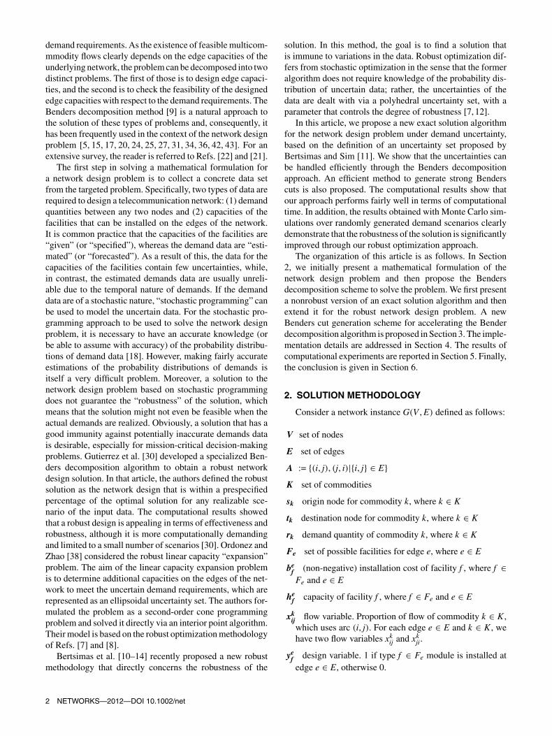
We now propose the “simultaneous Benders cut” scheme.In the classical Benders decomposition and all improvedmethods mentioned earlier, only one test solution y is used totest feasibility in the Benders subproblem, and the test solu-tion is obtained by solving the master problem to optimality.However, one frequent observation has been that there aremany integer solutions that are feasible to the current mas-ter problem and which have a slightly worse or even identicalobjective value. This observation implies that testing only onesolution may be too extreme, and to cut all of these similartest solutions off we may require many iterations of the mas-ter problem and the Benders subproblem, which in turn willresult in poor performance (see Fig. 1). Hence, it is desirable


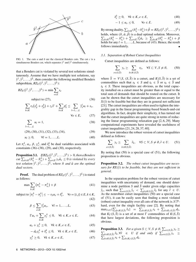
FIG. 1. The cuts a and b are the classical Benders cuts. The cut c is asimultaneous Benders cut, which separates y1 and y2 simultaneously.

that a Benders cut is violated by several test solutions simul-taneously. Assume that we have multiple test solutions, sayy1, y2, . . . , yL, then consider the following modified Benderssubproblem, RZX(y1, y2, . . . , yL):

RZX(y1, y2, . . . , yL) = min∑e∈E

se


rk(xk

ij + xkji

) + ze� +∑k∈K

pek ≤

∑l=1,...,L

yleul + se,

∀e ∈ E, (37)∑l=1,...,L

ul = 1, (38)

(29), (30), (31), (32), (33), (34), (39)

ul ≥ 0, ∀l = 1, . . . , L. (40)

Let πki , αe, β, γ k

e , and δke be dual variables associated with

constraints (36)–(38), (29), and (30), respectively.

Proposition 3.1. If RZX(y1, y2, . . . , yL) > 0, then a Benderscut

∑k∈K (π k

tk− π k

sk) + ∑

e∈E yeαe ≤ 0 is violated by everytest solution y1, y2, . . . , yL, where π and α are the optimaldual vectors.

Proof. The dual problem of RZX(y1, y2, . . . , yL) is statedas follows:

max∑k∈K

(π k

tk− π k

sk

) + β (41)

subject to∣∣π k

i − π kj

∣∣ ≤ − rkαe + δke , ∀e = {i, j} ∈ E, k ∈ K ,

(42)

β ≤∑e∈E

yleαe, ∀l = 1, . . . , L, (43)

�αe +∑k∈K

γ ke ≤ 0, ∀k ∈ K , e ∈ E, (44)

αe + γ ke ≤ 0, ∀k ∈ K , e ∈ E, (45)

− dkγke + δk

e ≤ 0, ∀k ∈ K , e ∈ E, (46)

γ ke ≥ 0, ∀k ∈ K , e ∈ E, (47)

δke ≥ 0, ∀k ∈ K , e ∈ E, (48)

− 1 ≤ αe ≤ 0, ∀e ∈ E. (49)

By strong duality,∑

k∈K (π ktk−π k

sk)+β = RZX(y1, y2, . . . , yL)

holds, where (π , α, β) is a dual optimal solution. Moreover,∑k∈K (π k

tk− π k

sk) + ∑

e∈E yleαe ≥ ∑

k∈K (π ktk

− π ksk) + β

holds for any l = 1, . . . , L, because of (43). Hence, the resultfollows immediately. ■

3.1. Separation of Robust Cutset Inequalities

Cutset inequalities are defined as follows:∑e∈(S,S)

ye ≥∑

k∈K(S,S)

rk , ∀S ⊂ V , S �= ∅, (50)

where S = V\S, (S, S) is a cutset, and K(S, S) is a set ofcommodities such that sk ∈ S and tk ∈ S or sk ∈ S andtk ∈ S. These inequalities are obvious, as the total capac-ity installed on a cutset must be greater than or equal to thetotal sum of demands that should be routed on the cutset. Itcan be shown that the cutset inequalities are necessary forX(y) to be feasible but that they are in general not sufficient[21]. The cutset inequalities are often used to tighten the inte-grality gap in the linear programming-based branch-and-cutalgorithms. In fact, despite their simplicity, it has turned outthat the cutset inequalities are quite strong in terms of reduc-ing the linear programming relaxation gap [2, 6, 29]. Manycomputational experiments have revealed the usefulness ofcutset inequalities [21, 24, 28, 37, 40].

We now introduce the robust version of cutset inequalitiesdefined as follows:∑

e∈(S,S)

ye ≥∑

k∈K(S,S)

rk , ∀S ⊂ V , S �= ∅, r ∈ U. (51)

By noting that (50) is a special case of (51), the followingproposition is obvious.

Proposition 3.2. The robust cutset inequalities are neces-sary for RX(y) to be feasible, but they are not sufficient ingeneral.

In the separation problem for the robust version of cutsetinequalities with uncertainty of demand, one should deter-mine a node partition S and S under given edge capacitiesye, such that

∑e∈(S,S) ye <

∑k∈K(S,S) rk for any r ∈ U.

As the nonrobust cutset inequalities (50) are a special caseof (51), it can be easily seen that finding a most violated(robust) cutset inequality over all cuts of the network is NP-hard, even for the single facility case [2]. By noting thatmaxr∈U{∑k∈K(S,S) rk} = ∑

k∈K(S,S) rk + ∑k∈K�(S,S) dk ,

that K�(S, S) is a set of at most � commodities of K(S, S)

that have largest deviations, the following proposition isobvious.

Proposition 3.3. For a given S ⊂ V , S �= ∅,∑

e∈(S,S) ye ≥∑k∈K(S,S) rk , ∀r ∈ U if and only if

∑e∈(S,S) ye ≥∑

k∈K(S,S) rk + ∑k∈K�(S,S) dk.


Here, we propose a heuristic algorithm based on the maxi-mum flow algorithm as follows. For each k ∈ K and the edgecapacities of a given test solution, we find a minimum sk − tkcut, say Sk , via the maximum flow algorithm, and then checkif the robust cutset inequality is satisfied by the (Sk , Sk) nodepartition in terms of the uncertainty of demand data—that is,we check if

∑e∈(Sk ,Sk)

ye <∑

k∈K(Sk ,Sk)rk +∑

k∈K�(Sk ,Sk)dk .

3.2. Simultaneous Robust Cutset Inequalities

When there are many test solutions, it is possible to obtain“simultaneous robust cutset inequalities,” which are robustcutset inequalities that are violated by multiple test solu-tions simultaneously. Let y∗

e := maxl∈L{yle} for a given

L ⊆ {1, . . . , L}.

Proposition 3.4. For any robust cutset inequality � definedby node partition S and S, � is violated by every test solutionl ∈ L if � is violated by the test solution y∗.

Proof. That � is violated by the test solution y∗ impliesthat

∑e∈(S,S) y∗

e <∑

k∈K(S,S) rk + ∑k∈K�(S,S) dk . Based

on the definition of y∗,∑

e∈(S,S) yle ≤ ∑

e∈(S,S) y∗e holds,

implying that∑

e∈(S,S) yle <

∑k∈K(S,S) rk + ∑

k∈K�(S,S) dk

for any l ∈ L. The result follows immediately. ■

We can find a robust cutset inequality which excludes morethan one test solution simultaneously. First, we identify aminimum sk − tk cut for each k ∈ K where the edge capaci-ties are given as “the edge-wise maximum of test solutions,”and then we check if the edge capacities violate the robust

cutset inequality defined by the minimum sk − tk cut. In thismanner, we are able to generate many robust cutset inequali-ties from many combinations of the test solutions. A detaileddescription of this approach is provided in the next section.

4. IMPLEMENTATION DETAILS

In this section, we provide a detailed description of thealgorithm implementation.

4.1. Initial Cutset Inequalities Generation

Before initiating the Benders decomposition iterations, anumber of cutset inequalities are added to the initial Bendersmaster problem. Without the initial cuts, the Benders masterproblem may produce too many unrealistic test solutions atthe early iterations [24,37]. To this end, we enumerate everysingle node and add a cutset inequality for each single nodeset—that is, for each node i and S = {i}, we add a cutsetinequality

∑e∈(S,S) ye ≥ ∑

k∈K(S,S) rk + ∑k∈K�(S,S) dk .

4.2. Cutset Inequality Generation Subproblem

Assume that we have L test solutions and they are sortedby their objective values—that is, i < j, if yi has a betterobjective value than yj for any i, j = 1, . . . , L.

The cutset generation algorithm is shown in Algorithm 1.First, we try to find the simultaneous robust cutset inequalitiesusing a new test solution y constructed by taking the edge-wise maximum of two test solutions yl and yq for anyl, q ∈ {1, . . . , L} and l �= q, that is, ye := max{yl

e, yqe }, ∀e ∈ E.

Note that we may attempt other combinations of the test,

Algorithm 1 Cutset inequalities generation

1: procedure GenCutsetCuts(y1, y2, . . . , yL, �) � ye = ∑f ∈Fe

hef ye

f , integer2: for k ∈ K do3: for l ∈ {1, 2, . . . , L − 1} do4: for q ∈ {l + 1, l + 2, . . . , L} do5: ye ← max{yl

e, yqe } for all e ∈ E. � Try to find a simultaneous cutset inequality for yl and yq.

6: S ← MinimumCut(k, y) � Maximum s − t flow algorithm7: if

∑e∈(S,S) ye <

∑k∈K(S,S) rk + ∑

k∈K�(S,S) dk then8: Add inequality

∑e∈(S,S)

∑f ∈Fe

hef ye

f ≥ ∑k∈K(S,S) rk + ∑

k∈K�(S,S) dk to the master problem9: end if

10: end for11: end for12: end for13: for l ∈ {1, 2, . . . , L} do14: for k ∈ K do15: S ← MinimumCut(k, yl) � Maximum s − t flow algorithm16: if

∑e∈(S,S) yl

e <∑

k∈K(S,S) rk + ∑k∈K�(S,S) dk then

17: Add inequality∑

e∈(S,S)

∑f ∈Fe

hef ye

f ≥ ∑k∈K(S,S) rk + ∑

k∈K�(S,S) dk to the master problem18: end if19: end for20: end for21: end procedure


solutions for finding new cutset inequalities, while the num-ber of the combinations is properly determined not to requiretoo much time in trying all of them. In Algorithm 1 the totalnumber of calls of MinimumCut algorithm is |K| × L(L−1)

2 ,and the max-flow problem can be solved very efficientlywith a specialized max-flow algorithm. We used a variantof the standard argumenting-path-based algorithm developedby Boykov and Kolmogorov [19]. If we failed to find anyviolated cutset inequality, then we executed the Benders cutgeneration procedure.

4.3. Benders Cuts Generation Subproblem

The Benders cut generation algorithm is shown in Algo-rithm 2. Starting from l = 1, we first try to find cuts thatsimultaneously violate test solutions y1, . . . , yl. If such asimultaneous Benders cut is identified, it is added to the mas-ter problem, and the procedure is repeated after increasing lby 1. If no such simultaneous cut is identified for test solutionsy1, . . . , yl∗ for some l = l∗, then we search for a classical Ben-ders cut for each test solution in a sequence from test solutionyl∗ up to yL. If a test solution happens to be feasible and thesolution is not the best test solution, we accept the solution as

Algorithm 2 Benders cuts generation

1: procedure GenBendersCuts(y1, y2, . . . , yL, �)� ye = ∑

f ∈Fehe

f yef , integer

2: l ← 13: repeat � Simultaneous Benders cut4: Solve RZX(y1, y2, . . . , yl) to optimality5: π , α ← the dual optimal vectors6: Z ← RZX(y1, y2, . . . , yl)

7: if Z > 0 then8: Add inequality

∑k∈K (π k

tk− π k

sk)

+ ∑e∈E αe

∑f ∈Fe

hef ye

f ≤ 0 to themaster problem

9: end if10: l ← l + 111: until Z = 0 or l > L12: if l ≤ L then13: repeat � Classical Benders cut14: Solve RZX(yl) to optimality15: π , α ← the dual optimal vectors16: Z ← RZX(yl)

17: if Z > 0 then18: Add inequality

∑k∈K (π k

tk− π k

sk)

+ ∑e∈E αe

∑f ∈Fe

hef ye

f ≤ 0to the master problem

19: else20: SaveIncumbent(yl)21: end if22: l ← l + 123: until Z = 0 or l > L24: end if25: end procedure

an incumbent solution. If the best test solution is feasible, wehave then obtained the true optimal solution for the networkdesign problem. It should be noted that, in classical Bendersdecomposition with a single test solution, it is impossible tohave an incumbent until the whole algorithm is terminated.

4.4. Benders Master Problem

At the current iteration l, the Benders master problem ispresented as follows:

min∑e∈E

∑f ∈Fe

bef ye

f (52)

subject to∑

e∈(Sj ,Sj)

ye ≥∑

k∈K(Sj ,Sj)

rk +∑

k∈K�(Sj ,Sj)

dk ,

∀j ∈ JInitial, (53)∑e∈(Sj ,Sj)

ye ≥∑

k∈K(Sj ,Sj)

rk +∑

k∈K�(Sj ,Sj)

dk ,

∀j ∈ JlCutset, (54)∑

k∈K

((π j)k

tk− (π j)k

sk

) +∑e∈E

αjeye ≤ 0,

∀j ∈ JlBenders, (55)

ye =∑f ∈Fe

hef ye

f , ∀e ∈ E, (56)

∑f ∈Fe

yef ≤ 1, ∀e ∈ E, (57)

∑e∈E

∑f ∈Fe

bef ye

f ≤ Z , (58)

yef ∈ {0, 1}, ∀f ∈ Fe, e ∈ E,

where JlCutset and Jl

Benders are the index sets of generated cutsetinequalities and Benders cuts thus far, respectively, whereasJInitial is the set of initially generated cutset inequalities. Wesolve the problem with a state-of-the-art MIP solver, such asCPLEX. If we have an incumbent solution, we add constraint(58) to prune branching nodes having worse objective valuesthan the incumbent value. The callback routine Incumbent-Callback, provided by CPLEX, was used to obtain multipletest solutions from the current master problem.

4.5. Benders Decomposition Algorithm

The overall Benders decomposition algorithm is givenin Algorithm 3. The cuts are generated in a hierarchicalsequence. As cutset inequalities are quite useful and can beidentified efficiently, we first try to find some cutset inequal-ities. When no cutset inequality is found, exact Benders cutsare generated. If no cuts at all are obtained by any of thecut generation routines, the current solution of the Bendersmaster problem is proved to be optimal.


Algorithm 3 Benders decomposition algorithm1: procedure RobustNetworkDesign(G(V , E), U, K , �)2: GenerateInitialCutset

3: l ← 04: repeat5: Solve current Benders master problem

� Using out-of-shelf MIP solver6: y1, y2, . . . , yL ← the test solutions7: GenCutsetCuts(y1, y2, . . . , yL, �)8: if no cutset is generated then9: GenBendersCuts(y1, y2, . . . , yL, �)

10: end if11: l ← l + 112: until no cut is generated13: end procedure

5. COMPUTATIONAL RESULTS

In this section, we present computational results for therobust network design problem. All computational tests pre-sented here were performed on an AMD X2 2.9 GHz PCwith 4GB RAM. The implementation of the algorithm wasdone with C + + with CPLEX 10.1 as the linear and integerprogramming solver.

5.1. Instances

We chose two test instances from SNDlib [39],which provides real-life telecommunication network designproblems. Characteristics of the test instances are given asfollows:

ta1–U-U-E-N-C-A-N-N : 24 nodes, 55 edges, 163 (undi-rected) demands, and 11 possible facilities on each edge.

norway–U-U-E-N-C-A-N-N : 27 nodes, 51 edges, 351(undirected) demands, and 2 possible facilities on eachedge.

These problems are very hard problems, and to the best of ourknowledge, they remain open for the optimal solutions evenfor the deterministic case (without uncertainty). We testedtwo cases for the maximum deviation values dk : 15% (dk =0.15rk for all k ∈ K) and 30% (dk = 0.30rk for all k ∈ K).

5.2. Performance Evaluation of the Proposed Algorithm

It is well known that the standard implementation ofthe Benders decomposition often does not work well. Here,we compare the performance of our algorithm with anotherenhanced Benders decomposition scheme proposed by Fis-chetti et al. [23], namely, the MIS Benders cut generationmethod. In our setting, the MIS Benders cuts can be obtainedwhen we modify the problem RZX(y) as follows:

min s (59)


rk(xk

ij + xkji

) + ze� +∑k∈K

pek ≤ ye + s, ∀e ∈ E,

(61)

(29) − (34), (62)

s ≥ 0. (63)

In other words, we replace every se with s in the problemRZX(y). Then, the dual of the above problem has the con-straint

∑e∈E αe ≤ 1, which regulates the values of αe so that

a small number of them are positive. It is noteworthy thatour simultaneous cut generation scheme is also applicable tothe MIS Benders cut generation method using multiple testsolutions. In this case, the MIS Benders cut replaces the exactBenders cuts.

In designing the Benders cut generation scheme, we haveseveral choices: (1) single cut generation versus multiple cutgeneration; (2) the use of the simultaneous cut generation (forboth the robust cutset inequalities and exact Benders cuts);and (3) the MIS Benders cut generation scheme. It shouldbe noted that our simultaneous cut generation scheme is notbound to any one specific Benders subproblem formulation.In other words, we can consider simultaneous versions of anyBenders subproblems, such as the exact Benders cut gen-eration, the robust cutset generation, and the MIS Benderscut generation. Here, we consider six different combina-tions of cut generation schemes to investigate their effectsindependently.

Single test solution: Robust cutset generation + exact Ben-ders cut generation with single test solution (the classicalBenders decomposition approach).

Single test solution (MIS): Robust cutset generation + MISBenders cut generation with single test solution.

Multiple test solutions: Robust cutset generation + exactBenders cut generation with multiple test solutions (butwithout simultaneous cut generation).

Multiple test solutions: Simultaneous robust cutset gener-ation + simultaneous exact Benders cut generation withmultiple test solutions.

Multiple test solutions (MIS): Robust cutset generation +MIS Benders cut generation with multiple test solutions(but without simultaneous cut generation).

Multiple test solutions (MIS): Simultaneous robust cutsetgeneration + simultaneous MIS Benders cut generationwith multiple test solutions.

It is also possible to use only the exact Benders cut scheme (orMIS Benders cut) without robust cutset inequalities. We havealso tested this approach, but the performance was so pooreven with the simultaneous cuts we were unable to obtainany optimal solution by this approach within the 3-h time


TAB

LE

1.R

esul

tsof

prop

osed

algo

rith

mfo

rne

twor

kta1

.

d

Sing

lete

stso

lutio

nSi

ngle

test

solu

tion

(MIS

)M

utip

lete

stso

lutio

nsM

utip

lete

stso

lutio

nsM

utip

lete

stso

lutio

ns(M

IS)

Mut

iple

test

solu

tions

(MIS

)C

plex

Opt

imal

gap

Inc

(%)

�#i

ter

Tim

e#c

ut(#

bc)

#ite

rT

ime

#cut

(#bc

)#i

ter

Tim

e#c

ut(#

bc)

#ite

rT

ime

#cut

(#bc

)#i

ter

Tim

e#c

ut(#

bc)

#ite

rT

ime

#cut

(#bc

)(%

)T

ime

Val

ue(%

)

15

025

10.6

244(

0)25

12.8

244(

0)15

12.0

351(

0)12

22.1

351(

0)15

13.7

351(

0)12

23.9

351(

0)20

.910

,800

∗7,

518,

317

0.00

121

20.1

211(

1)24

146.

023

4(1)

1110

.731

0(0)

1125

.333

5(0)

1139

.431

0(0)

1153

.133

5(0)

27.4

10,8

00∗

7,54

7,80

00.

392

2510

7.1

237(

5)15

316.

314

2(2)

2048

.727

3(5)

2240

.127

3(3)

1213

0.2

221(

3)14

112.

721

6(1)

36.1

10,8

00∗

7,56

2,54

20.

593

2672

.222

2(5)

1834

6.8

193(

2)21

57.8

301(

4)18

38.5

375(

3)15

264.

028

6(2 )

1210

5.0

251(

1)27

.110

,800

∗7,

562,

542

0.59

432

19.2

260(

3)22

188.

818

5(1)

2020

.727

3(4)

1838

.337

7(3)

1397

.122

3(1)

1311

5.6

367(

1)28

.610

,800

∗7,

562,

542

0.59

521

14.3

185(

2)17

113.

615

3(1)

1311

.126

9(1)

1427

.624

8(3)

1212

2.7

247(

1)9

79.4

229(

1)32

.010

,800

∗7,

562,

542

0.59

619

15.6

163(

2)15

79.2

134(

1)19

18.3

318(

3)17

36.6

277(

4)11

76.1

199(

1)11

155.

123

7(1)

38.2

10,8

00∗

7,56

2,54

20.

597

2233

.319

8(3)

1933

3.2

172(

2)15

33.2

254(

2)18

58.8

378(

3)14

323.

423

9(2)

1212

9.8

292(

1)32

.010

,800

∗7,

562,

542

0.59

827

191.

219

5(6)

2131

2.4

188(

2)18

86.3

280(

3)19

72.2

370(

4)12

125.

423

9(1)

1010

2.3

256(

1)33

.610

,800

∗7,

562,

542

0.59

924

16.4

194(

2)22

91.3

191(

1)18

26.0

328(

3)20

66.1

450(

5)13

177.

330

4(1)

1118

5.5

340(

1)38

.410

,800

∗7,

562,

542

0.59

30

137

74.5

290(

6)22

258.

820

7(2)

2117

.937

8(4)

1739

.527

4(5)

1122

7.5

255(

1)12

237.

927

8(1)

26.3

10,8

00∗

7,56

2,54

20.

592

2117

.918

5(2)

1875

.217

2(1)

1820

.935

2(3)

1019

.636

9(0)

1310

0.0

324(

1)10

36.3

369(

0)29

.810

,800

∗7,

562,

542

0.59

329

31.6

222(

5)23

367.

719

4(2)

1820

.634

3(3)

916

.929

2(0)

1114

6.0

226(

1)9

32.8

292(

0)23

.410

,800

∗7,

562,

542

0.59

429

38.4

209(

6)21

237.

417

8(2)

2028

.138

0(3)

1839

.128

5(3)

1312

1.5

292(

1)11

124.

425

7(1)

20.8

10,8

00∗

7,56

2,54

20.

595

1919

.216

0(3)

1512

2.2

143(

1)10

5.3

229(

0)12

41.8

299(

3)10

21.8

229(

0)8

375.

219

4(2)

23.3

10,8

00∗

7,56

2,54

20.

596

3024

.527

2(3)

1718

0.5

159(

1)15

21.1

324(

2)20

43.3

281(

5)11

155.

322

0(1)

1014

0.4

170(

1)20

.810

,800

∗7,

562,

542

0.59

711

3.2

106(

0)11

16.6

106(

0)12

5.6

234(

0)16

41.0

293(

5)12

21.2

234(

0)10

133.

525

9(3)

18.8

10,8

00∗

7,56

2,54

20.

598

92.

310

1(0)

916

.210

1(0)

2139

.638

6(4)

1735

.920

9(3)

1213

5.4

263(

1)11

133.

318

2(1)

22.6

10,8

00∗

7,56

2,54

20.

599

2419

.419

6(4)

1515

8.2

125(

1)17

46.1

261(

6)7

8.2

174(

0)11

102.

422

8 (1)

722

.417

4(0)

24.4

10,8

00∗

7,56

2,54

20.

59A

vg.

23.7

38.5

202.

6(3.

1)18

.417

7.5

169.

5(1.

2)16

.927

.930

7.6(

2.6)

15.5

37.4

311.

1(2.

7)12

.212

6.3

257.

4(1.

0)10

.712

1.0

265.

7(0.

9)27

.610

,800

∗


TAB

LE

2.R

esul

tsof

prop

osed

algo

rith

mfo

rne

twor

knorway

.

d

Sing

lete

stso

lutio

nSi

ngle

test

solu

tion

(MIS

)M

utip

lete

stso

lutio

nsM

utip

lete

stso

lutio

nsM

utip

lete

stso

lutio

ns(M

IS)

Mut

iple

test

solu

tions

(MIS

)C

plex

Opt

imal

gap

Inc

(%)�

#ite

rT

ime

#cut

(#bc

)#i

ter

Tim

e#c

ut(#

bc)

#ite

rT

ime

#cut

(#bc

)#i

ter

Tim

e#c

ut(#

bc)

#ite

rT

ime

#cut

(#bc

)#i

ter

Tim

e#c

ut(#

bc)

(%)

Tim

eV

alue

(%)

15

079

10,8

00∗

910(

4)74

10,8

00∗

808(

2)28

9,49

9.5

1,05

2(0)

193,

564.

01,

165(

0)28

9,68

2.4

1,05

2(0)

193,

602.

91,

165(

0)47

.810

,800

∗45

2,68

00.

001

8010

,800

∗95

0(4)

7310

,800

∗76

6(1)

212,

818.

61,

011(

0)16

2,82

6.6

1,02

1(0)

212,

963.

71,

011(

0)16

2,87

6.5

1,02

1(0)

58.5

10,8

00∗

452,

680

0.00

273

10,8

00∗

884(

6)69

10,8

00∗

696(

4)32

10,4

60.7

1,29

1(0)

185,

146.

01,

240(

0)32

10,4

67.5

1,29

1(0)

185,

106.

91,

240(

0)58

.110

,800

∗45

4,85

00.

483

7110

,800

∗77

4(5)

6010

,800

∗72

5(4)

276,

235.

11,

285(

0)18

3,74

5.8

1,27

6(0)

276,

235.

61,

285(

0)18

3,88

0.2

1,27

6(0)

61.9

10,8

00∗

454,

850

0.48

465

10,8

00∗

747(

1)59

10,8

00∗

803(

2)24

4,42

6.2

1,13

8(0)

193,

530.

41,

073(

0)24

4,43

9.7

1,13

8(0)

193,

476.

11,

073(

0)54

.410

,800

∗45

4,85

00.

485

6310

,800

∗90

1(2)

5910

,800

∗87

5(1)

243,

853.

91,

111(

0)14

2,44

1.9

1,03

4(0)

243,

964.

41,

111(

0)14

2,47

3.3

1,03

4(0)

56.7

10,8

00∗

454,

850

0.48

662

10,8

00∗

928(

1)60

10,8

00∗

881(

1)24

3,83

2.1

1,11

1(0 )

142,

479.

71,

034(

0)24

3,88

3.4

1,11

1(0)

142,

493.

41,

034(

0)56

.210

,800

∗45

4,85

00.

487

6610

,800

∗89

5(1)

6210

,800

∗90

8(1)

243,

824.

11,

111(

0)14

2,44

6.1

1,03

4(0)

243,

812.

81,

111(

0)14

2,43

7.9

1,03

4(0)

58.3

10,8

00∗

454,

850

0.48

863

10,8

00∗

916(

1)59

10,8

00∗

868(

1)24

3,81

6.4

1,11

1(0)

142,

405.

51,

034(

0)24

3,86

6.4

1,11

1(0)

142,

474.

71,

034(

0)56

.310

,800

∗45

4,85

00.

489

6310

,800

∗89

5(1)

5910

,800

∗88

4(1)

243,

965.

71,

111(

0)14

2,41

5.2

1,03

4(0)

243,

951.

11,

111(

0)14

2,57

7.7

1,03

4(0)

59.4

10,8

00∗

454,

850

0.48

30

175

10,8

00∗

777(

4)66

10,8

00∗

715(

2)33

10,8

00*

1,51

6(0)

184,

100.

01,

004(

0)33

10,8

00*

1,51

6(0)

184,

154.

81,

004(

0)58

.010

,800

∗45

4,85

00.

482

7310

,800

∗87

9(2)

6210

,800

∗70

1(5)

277,

763.

495

8(0)

194,

332.

51,

161(

0)27

7,73

9.0

958(

0)19

4,30

8.4

1,16

1(0)

57.5

10,8

00∗

454,

850

0.48

374

10,8

00∗

894(

0)76

10,8

00∗

900(

0)30

10,1

60.3

1,13

1(1)

194,

853.

31,

233(

0)32

10,6

99.4

1,15

9(1)

194,

940.

21,

233(

0)56

.010

,800

∗45

4,85

00.

484

6910

,800

∗83

3(0)

6910

,800

∗83

3(0)

2610

,156

.81,

264(

0)14

1,62

3.5

911(

0)26

10,2

03.9

1,26

4(0)

141,

674.

191

1(0)

54.6

10,8

00∗

454,

850

0.48

572

10,8

00∗

919(

1)60

10,8

00∗

913(

2)21

3,06

1.8

952(

0)17

4,46

2.1

1,16

5(0)

213,

052.

195

2(0)

174,

586.

11,

165(

0)50

.210

,800

∗45

4,85

00.

486

5710

,800

∗74

1(0)

5710

,800

∗74

1(0)

306,

847.

41,

091(

0)15

4,86

3.0

1,05

4(0)

306,

948.

81,

091(

0)15

4,93

3.2

1,05

4(0)

58.6

10,8

00∗

454,

850

0.48

755

10,8

00∗

777(

0)55

10,8

00∗

777(

0)25

10,8

00*

1,04

9(0)

193,

848.

51,

155(

0)25

10,8

00*

1,04

9(0)

193,

892.

11,

155(

0)53

.610

,800

∗45

4,85

00.

488

5910

,800

∗88

7(0)

5910

,800

∗88

7(0)

286,

897.

31,

122(

0)17

2,93

4.9

976(

0)28

6,79

3.7

1,12

2(0)

172,

947.

097

6(0)

53.9

10,8

00∗

454,

850

0.48

956

10,8

00∗

736(

2)52

10,8

00∗

737(

2)28

6,24

7.2

960(

1)19

5,01

8.0

805(

1)28

6,01

6.8

966(

1)19

5,31

8.6

805(

1)55

.410

,800

∗45

4,85

00.

48A

vg.

67.1

10,8

00∗

854.

9(1.

8)62

.610

,800

∗81

1.5(

1.5)

26.3

6,64

5.3

1,12

5.0(

0.1)

16.7

3,52

8.3

1,07

4.2(

0.1)

26.4

6,68

7.3

1,12

6.8(

0.1)

16.7

3,58

7.1

1,07

4.2(

0.1)

56.1

10,8

00∗


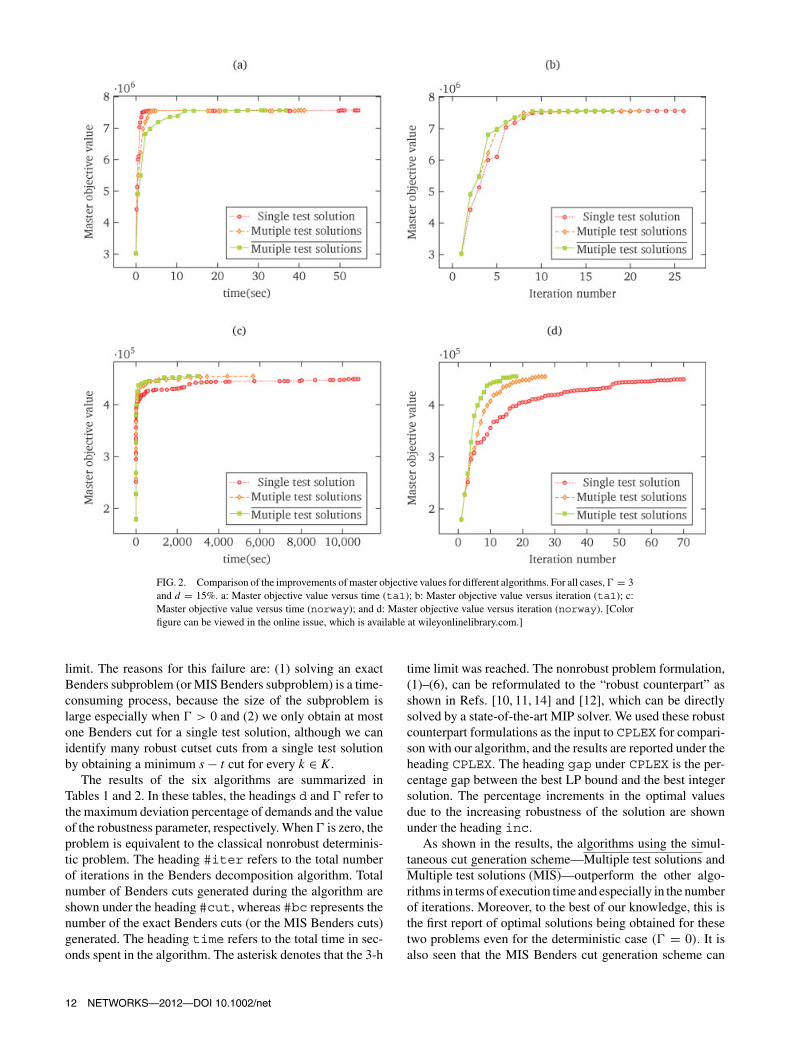
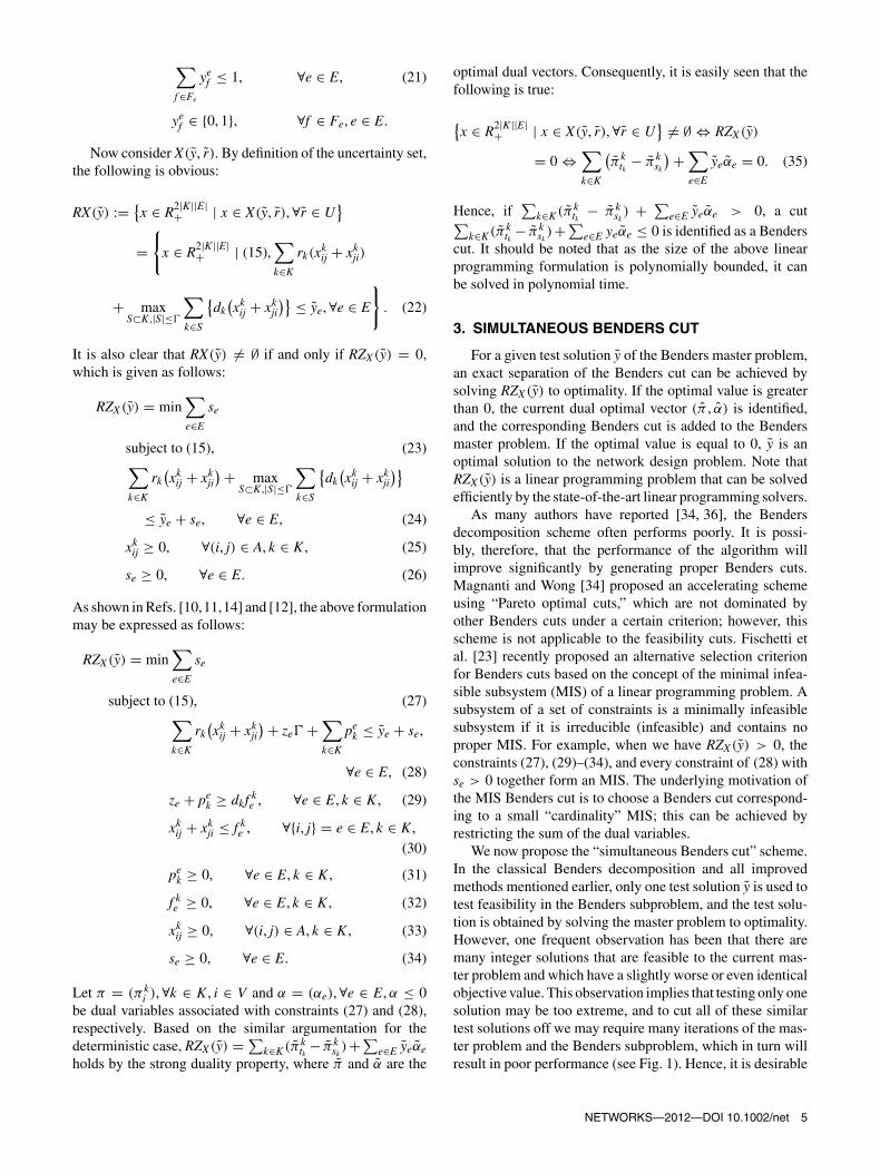
FIG. 2. Comparison of the improvements of master objective values for different algorithms. For all cases, � = 3and d = 15%. a: Master objective value versus time (ta1); b: Master objective value versus iteration (ta1); c:Master objective value versus time (norway); and d: Master objective value versus iteration (norway). [Colorfigure can be viewed in the online issue, which is available at wileyonlinelibrary.com.]

limit. The reasons for this failure are: (1) solving an exactBenders subproblem (or MIS Benders subproblem) is a time-consuming process, because the size of the subproblem islarge especially when � > 0 and (2) we only obtain at mostone Benders cut for a single test solution, although we canidentify many robust cutset cuts from a single test solutionby obtaining a minimum s − t cut for every k ∈ K .

The results of the six algorithms are summarized inTables 1 and 2. In these tables, the headings d and � refer tothe maximum deviation percentage of demands and the valueof the robustness parameter, respectively. When � is zero, theproblem is equivalent to the classical nonrobust determinis-tic problem. The heading #iter refers to the total numberof iterations in the Benders decomposition algorithm. Totalnumber of Benders cuts generated during the algorithm areshown under the heading #cut, whereas #bc represents thenumber of the exact Benders cuts (or the MIS Benders cuts)generated. The heading time refers to the total time in sec-onds spent in the algorithm. The asterisk denotes that the 3-h

time limit was reached. The nonrobust problem formulation,(1)–(6), can be reformulated to the “robust counterpart” asshown in Refs. [10, 11, 14] and [12], which can be directlysolved by a state-of-the-art MIP solver. We used these robustcounterpart formulations as the input to CPLEX for compari-son with our algorithm, and the results are reported under theheading CPLEX. The heading gap under CPLEX is the per-centage gap between the best LP bound and the best integersolution. The percentage increments in the optimal valuesdue to the increasing robustness of the solution are shownunder the heading inc.

As shown in the results, the algorithms using the simul-taneous cut generation scheme—Multiple test solutions andMultiple test solutions (MIS)—outperform the other algo-rithms in terms of execution time and especially in the numberof iterations. Moreover, to the best of our knowledge, this isthe first report of optimal solutions being obtained for thesetwo problems even for the deterministic case (� = 0). It isalso seen that the MIS Benders cut generation scheme can


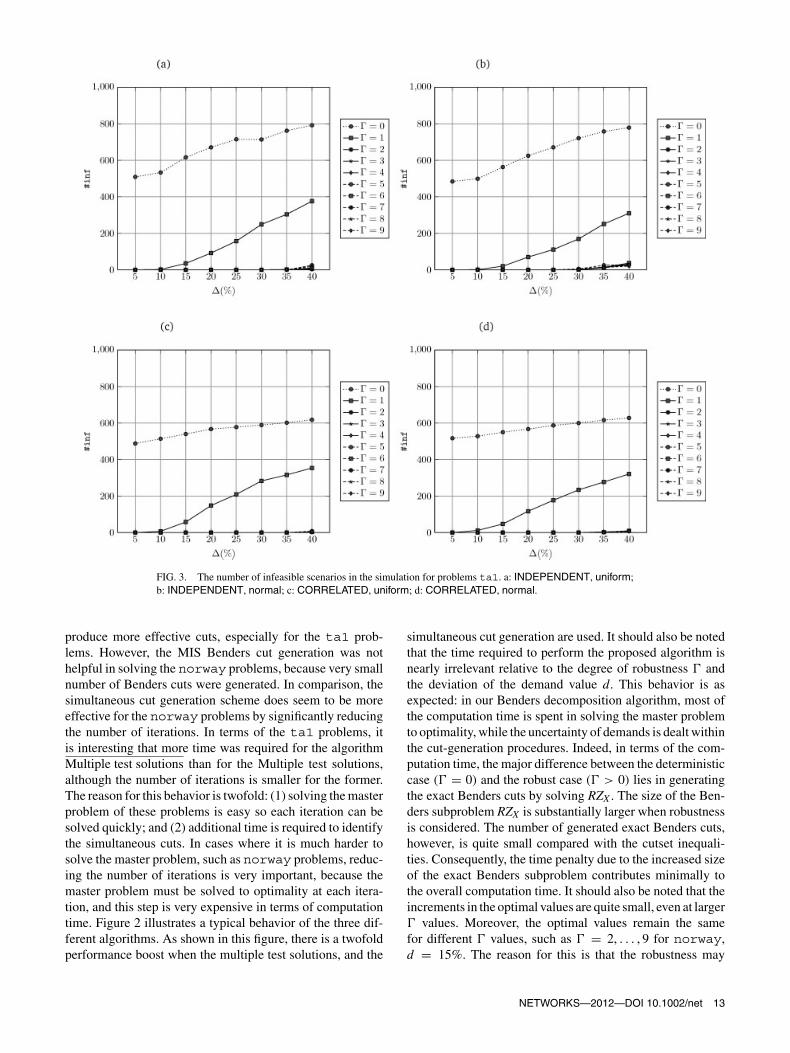
FIG. 3. The number of infeasible scenarios in the simulation for problems ta1. a: INDEPENDENT, uniform;b: INDEPENDENT, normal; c: CORRELATED, uniform; d: CORRELATED, normal.

produce more effective cuts, especially for the ta1 prob-lems. However, the MIS Benders cut generation was nothelpful in solving the norway problems, because very smallnumber of Benders cuts were generated. In comparison, thesimultaneous cut generation scheme does seem to be moreeffective for the norway problems by significantly reducingthe number of iterations. In terms of the ta1 problems, itis interesting that more time was required for the algorithmMultiple test solutions than for the Multiple test solutions,although the number of iterations is smaller for the former.The reason for this behavior is twofold: (1) solving the masterproblem of these problems is easy so each iteration can besolved quickly; and (2) additional time is required to identifythe simultaneous cuts. In cases where it is much harder tosolve the master problem, such as norway problems, reduc-ing the number of iterations is very important, because themaster problem must be solved to optimality at each itera-tion, and this step is very expensive in terms of computationtime. Figure 2 illustrates a typical behavior of the three dif-ferent algorithms. As shown in this figure, there is a twofoldperformance boost when the multiple test solutions, and the

simultaneous cut generation are used. It should also be notedthat the time required to perform the proposed algorithm isnearly irrelevant relative to the degree of robustness � andthe deviation of the demand value d. This behavior is asexpected: in our Benders decomposition algorithm, most ofthe computation time is spent in solving the master problemto optimality, while the uncertainty of demands is dealt withinthe cut-generation procedures. Indeed, in terms of the com-putation time, the major difference between the deterministiccase (� = 0) and the robust case (� > 0) lies in generatingthe exact Benders cuts by solving RZX . The size of the Ben-ders subproblem RZX is substantially larger when robustnessis considered. The number of generated exact Benders cuts,however, is quite small compared with the cutset inequali-ties. Consequently, the time penalty due to the increased sizeof the exact Benders subproblem contributes minimally tothe overall computation time. It should also be noted that theincrements in the optimal values are quite small, even at larger� values. Moreover, the optimal values remain the samefor different � values, such as � = 2, . . . , 9 for norway,d = 15%. The reason for this is that the robustness may


FIG. 4. The number of infeasible scenarios in the simulation for problems norway. a: INDEPENDENT,uniform; b: INDEPENDENT, normal; c: CORRELATED, uniform; d: CORRELATED, normal.

be obtained through alternate routing of flows on the samenetwork design.

5.3. Monte Carlo Simulation Tests

In real-life situations, it is clear that the uncertainties ofdemands are not restricted to the uncertainty set defined by �and d. The expectation is that the robust solutions based onour definition of uncertainty set may also be robust in morecomplicated uncertainties of real-life situations. To validatethis expectation, we conducted Monte Carlo simulation teststhat were designed to mimic real-life situations. As such,let rk denote the nominal demand value for commodity k.We assume that the (unknown) probability distribution forthe uncertain demand follows a normal distribution (N ) ora uniform distribution (U). Depending on combinations ofsimulation conditions, we considered four cases. For a givensimulation parameter :

Normal distribution; INDEPENDENT case: We assume thatthe demand value for k ∈ K obeys a normal distributionN (rk , (k/2)2), where k = rk.

Normal distribution; CORRELATED case: We assume thatyi, i ∈ V , obeys a normal distributionN (0, (/2

√2)2), which

is realized as yi. The demand of commodity k is set to rk +rk(ysk + ytk ), where sk and tk are the origin and the destinationnode, respectively.Uniform distribution; INDEPENDENT case: We assume thatthe demand value for k ∈ K obeys a uniform distributionU(rk − k , rk + k), where k = rk.Uniform distribution; CORRELATED case: We assume thatyi, i ∈ V , obeys a uniform distribution U(−/2, /2), whichis realized as yi. The demand of commodity k is set to rk +rk(ysk + ytk ), where sk and tk are the origin and the destinationnode, respectively.

In the INDEPENDENT case, we assumed that the probabil-ity distributions of demands are independent of each other.Note that P(rk − k ≤ rk ≤ rk + k) is about 95% for thenormal distribution and 100% for the uniform distribution. Inthe CORRELATED case, we assumed that demands with thesame origin node and/or destination node are positively cor-related. In this case, the uncertainties are not considered in


the commodity-wise context but in the node-wise context.For each problem and demand type, we randomly gener-ated 1,000 demand data scenarios for each given . Aftergenerating the demand scenarios, we could easily check thefeasibility of the optimal solutions for the demand scenarios.

The results of the simulation tests are reported in Figures3 and 4 for different values of �. The demand deviation valued was 30% for all problems. In these figures, the vertical axis#inf refers to the number of infeasible instances out of atotal 1,000 scenarios for each test case. The results clearlyshow that the robustness of the solutions is greatly improvedby our algorithm, even at the smallest protection level. Thedeterministic solutions were in particular highly unreliable,with more than 80% of the scenarios being infeasible for thedeterministic solutions. It should be noted that the penaltiesin the objective values are less than 1% at every protec-tion level � ≤ 9, while the robustness of the solutions issignificantly improved. It is also observable that both cases ofINDEPENDENT and CORRELATED show similar results.

6. CONCLUSIONS

In this article, we proposed an exact solution approachbased on the Benders decomposition scheme for the robustnetwork design problem. The most crucial constraint in thenetwork design problem is the guarantee that all multi-commodity flows of the demands are delivered. However,uncertainties in demand data are inevitable in real-life situa-tions, leading to the very likely possibility that the solutionmay not be robust under different realizations of demands.To handle this uncertainty, we defined the uncertainty set ofdemand data and proposed a decomposition approach thatseparates the uncertainty from the design problem (Ben-ders master problem). A robust version of feasibility testproblems (Benders subproblems) was then derived to ensurethe feasibility of multicommodity flows, and efficient solu-tion methods for the Benders subproblems were proposed.We also showed that the Benders decomposition algorithmcan be accelerated by the simultaneous Benders cut, whichexcludes several test solutions simultaneously. The compu-tational results showed that our algorithm performs welland can produce more robust solutions within a reasonableamount of time. The results of the simulation tests clearlyshowed that the improvements in robustness are significant,whereas the penalties in the objective value are very small.

Acknowledgments

The authors thank the anonymous referees for their helpfuland constructive comments.

REFERENCES

[1] R.K. Ahuja, T.L. Magnanti, and J.B. Orlin, Network flows,Prentice Hall, New Jersey, 1993.

[2] A. Atamtürk, On capacitated network design cut-set polyhe-dra, Math Program 92 (2002), 425–437.

[3] A. Atamtürk and D. Rajan, On splittable and unsplittable flowcapacitated network design arc-set polyhedra, Math Program92 (2002), 315–333.

[4] P. Avella, S. Mattia, and A. Sassano, Metric inequalitiesand the network loading problem, Discr Optim 4 (2007),103–114.

[5] A. Balakrishnan, T.L. Magnanti, and R.T. Wong, A decompo-sition algorithm for local access telecommunications networkexpansion planning, Oper Res 43 (1995), 58–76.

[6] F. Barahona, Network design using cut inequalities, SIAM JOptim 6 (1996), 823–837.

[7] A. Ben-Tal and A. Nemirovski, Robust convex optimization,Math Oper Res 23 (1998), 769–805.

[8] A. Ben-Tal and A. Nemirovski, Robust solutions of linearprogramming problems contaminated with uncertain data,Math Program 88 (2000), 411–424.

[9] J. Benders, Partitioning procedures for solving mixed-variables programming problems, Numer Mathematik 4(1962), 238–252.

[10] D. Bertsimas, D. Pachamanova, and M. Sim, Robust linearoptimization under general norms, Oper Res Lett 32 (2004),510–516.

[11] D. Bertsimas and M. Sim, Robust discrete optimization andnetwork flows, Math Program 98 (2003), 49–71.

[12] D. Bertsimas and M. Sim, The price of robustness, Oper Res52 (2004), 35–53.

[13] D. Bertsimas and A. Thiele, “A robust optimization approachto supply chain management,” Integer Programming andCombinatorial Optimization: 10th International IPCO Con-ference, New York, NY, Proceedings, Vol. 10, Springer, NewYork, 2004, pp. 86–100.

[14] D. Bertsimas and R. Weismantel, Optimization over integers,Dynamic Ideas, Massachusetts, 2005.

[15] D. Bienstock, S. Chopra, O. Günlük, and C.Y. Tsai, Minimumcost capacity installation for multicommodity network flows,Math Program 81 (1998), 177–199.

[16] D. Bienstock and O. Günlük, Capacitated network design-polyhedral structure and computation, INFORMS J Comput8 (1996), 243–259.

[17] S. Binato, M.V.F. Pereira, and S. Granville, A new Bendersdecomposition approach to solve power transmission net-work design problems, IEEE Trans Power Syst 16 (2001),235–240.

[18] J.R. Birge and F. Louveaux, “Introduction to stochastic pro-gramming,” Springer series in operations research, Springer,New York, 1997.

[19] Y. Boykov and V. Kolmogorov, An experimental compari-son of min-cut/max-flow algorithms for energy minimizationin vision, IEEE Trans Pattern Anal Machine Intelligence 26(2004), 1124–1137.

[20] J.F. Cordeau, F. Pasin, and M.M. Solomon, An integratedmodel for logistics network design, Ann Oper Res 144(2006), 59–82.

[21] A. Costa, J. Cordeau, and B. Gendron, Benders, metric andcutset inequalities for multicommodity capacitated networkdesign, Comput Optim Appl 42 (2007), 371–392.

[22] A.M. Costa, A survey on Benders decomposition applied tofixed-charge network design problems, Comput Oper Res 32(2005), 1429–1450.


[23] M. Fischetti, D. Salvagnin, and A. Zanette, A note on theselection of Benders’ cuts, Math Program 124 (2010), 1–8.

[24] V. Gabrel, A. Knippel, and M. Minoux, Exact solution of mul-ticommodity network optimization problems with generalstep cost functions, Oper Res Lett 25 (1999), 15–23.

[25] V. Gascon, A. Benchakroun, and J.A. Ferland, Electricity dis-tribution planning-model—A network design approach forsolving the master problem of the Benders decompositionmethod, INFOR 31 (1993), 205–220.

[26] B. Gendron, T. Crainic, and A. Frangioni, “Multicommoditycapacitated network design,” Telecommunications networkplanning, B. Sansó and P. Soriano (Editors), Springer, NewYork, 1998, pp. 1–19.

[27] A.M. Geoffrion and G.W. Graves, Multicommodity distribu-tion system design by Benders decomposition, Manage Sci20 (1974), 822–844.

[28] J.A. Gomez and W. Gomez, Cutting plane algorithms forrobust conic convex optimization problems, Optim MethodsSoftware 21 (2006), 779–803.

[29] O. Günlük, A branch-and-cut algorithm for capacitatednetwork design problems, Math Program 86 (1999), 17–39.

[30] G.J. Gutierrez, P. Kouvelis, and A.A. Kurawarwala, A robust-ness approach to uncapacitated network design problems, EurJ Oper Res 94 (1996), 362–376.

[31] M. Haouari, M. Mrad, and H.D. Sherali, Optimum synthesisof discrete capacitated networks with multi-terminal com-modity flow requirements, Optim Lett 1 (2007), 341–354.

[32] A. Knippel and B. Lardeux, The multi-layered networkdesign problem, Eur J Oper Res 183 (2007), 87–99.

[33] T.L. Magnanti, P. Mirchandani, and R. Vachani, Model-ing and solving the two-facility capacitated network loadingproblem, Oper Res 43 (1995), 142–157.

[34] T.L. Magnanti and R.T. Wong, Accelerating Benders decom-position: Algorithmic enhancement and model selectioncriteria, Oper Res 29 (1981), 464–484.

[35] T.L. Magnanti and R.T. Wong, Network design and trans-portation planning: Models and algorithms, Transport Sci 18(1984), 1–55.

[36] T.L. Magnanti, R.T. Wong, and P. Mireault, Tailoring Ben-ders decomposition for uncapacitated network design, MathProgram Study 26 (1986), 112–154.

[37] M. Mrad and M. Haouari, Optimal solution of the discretecost multicommodity network design problem, Appl MathComputation 204 (2008), 745–753.

[38] F. Ordonez and J.M. Zhao, Robust capacity expansion ofnetwork flows, Networks 50 (2007), 136–145.

[39] S. Orlowski, R. Wessäly, M. Pióro, and A. Tomaszewski,SNDlib 1.0—Survivable Network Design Library, Networks55 (2010), 276–286.

[40] C. Raack, A. Koster, S. Orlowski, and R. Wessäly, On cut-based inequalities for capacitated network design polyhedra,Networks 57 (2011), 141–156.

[41] R.L. Rardin and L.A. Wolsey, Valid inequalities and project-ing the multicommodity extended formulation for uncapaci-tated fixed charge network flow problems, Eur J Oper Res 71(1993), 95–109.

[42] V. Sridhar and J.S. Park, Benders-and-cut algorithm for fixed-charge capacitated network design problem, Eur J Oper Res125 (2000), 622–632.

[43] H. Uster, G. Easwaran, E. Akcali, and S. Cetinkaya, Bendersdecomposition with alternative multiple cuts for a multi-product closed-loop supply chain network design model,Naval Res Logist 54 (2007), 890–907.


Documents

Benders decomposition approach for the robust network