Benchmarking systems of seasonally adjusted time

series according to Denton’s movement preservation

principle

T. Di Fonzo and M. Marini

2003.09

Abstract When a system of time series is seasonally adjusted, generally the accounting constraints originally linking the series are not fulfilled. To overcome this problem, we discuss an extension to a system of series linked by an accounting constraint of the classical univariate benchmarking procedure due to Denton (1971), which is founded on a movement preservation principle very appreciable in this case. The presence of linear dependence between the variables makes it necessary to conveniently deal with the whole set of contemporaneous and temporal aggregation relationships. The cases of one-way classified (e.g., by regions or by industries) and of two-ways classified (e.g., by regions and by industries) systems of series are studied. Moreover, simplified expressions of the matrices involved in the calculations are presented, which turn out useful in practical implementation of benchmarking for large systems of series. An empirical application to the Canadian retail trade series by province (12 series) and trade groups (18 series) is finally considered to show the capability of the proposed procedures.

Keywords: benchmarking; systems of time series; accounting constraints; Denton’s movement preservation principle.

1

Benchmarking systems of seasonally adjusted time series according to Denton’s movement preservation principle

Tommaso Di Fonzo Marco Marini

Dipartimento di Scienze Statistiche Università di Padova

Istituto Nazionale di Statistica Roma

Index 1. Introduction..................................................................................................................................2 2. Statement of the problem and some notation...............................................................................3 3. One system of series and a binding accounting constraint ..........................................................4 4. The benchmarking formula..........................................................................................................6 5. The choice of Ω : Denton’s movement preservation principle....................................................8

5.1. One system of series and an unbinding accounting constraint ..........................................10 6. Benchmarking two systems of time series linked by an accounting constraint.........................11

6.1. Binding constraint ..............................................................................................................11 6.2. Unbinding (and unavailable preliminary estimate) constraint...........................................14 6.3. Unbinding constraint with an available preliminary estimate ...........................................14

Simplified expressions using partitioned matrices ....................................................................16 7. Benchmarking while preserving period-to-period growth rates ................................................17 8. Benchmarking a system of two-ways classified series ..................................................................20

8.1. A system of two-ways classified series with binding constraints......................................22 8.2. A system of two-ways classified series with neither binding nor preliminary constraints23

9. An evaluation of computational times on simulated data ..........................................................24 10. An application: benchmarking Canadian retail trade seasonally adjusted series by province and

trade groups...............................................................................................................................26 10.1. Benchmarking series by province......................................................................................29 10.2. Simultaneous benchmarking of series by province and trade groups................................31

Appendix: Derivation of the Moore-Penrose generalized inverse of 'a =Ω HΩH ..........................34 References..........................................................................................................................................35 Summary When a system of time series is seasonally adjusted, generally the accounting constraints originally linking the series are not fulfilled. To overcome this problem, we discuss an extension to a system of series linked by an accounting constraint of the classical univariate benchmarking procedure due to Denton (1971), which is founded on a movement preservation principle very appreciable in this case. The presence of linear dependence between the variables makes it necessary to conveniently deal with the whole set of contemporaneous and temporal aggregation relationships. The cases of one-way classified (e.g., by regions or by industries) and of two-ways classified (e.g., by regions and by industries) systems of series are studied. Moreover, simplified expressions of the matrices involved in the calculations are presented, which turn out useful in practical implementation of benchmarking for large systems of series. An empirical application to the Canadian retail trade series by province (12 series) and trade groups (18 series) is finally considered to show the capability of the proposed procedures. Keywords: benchmarking; systems of time series; accounting constraints; Denton’s movement preservation principle. Acknowledgments: T.D.F. was partially supported by grants from MIUR and University of Padova. July 2003

2

1. Introduction

Laniel and Fyfe (1989, pp. 464-465) write:

Most economic sub-annual surveys produce series of estimates for a number of industrial activities within a number of geographical regions. These are published sub-annually in the form of tables, where the cells as well as the marginals and the grand totals need to be benchmarked. If one applies a benchmarking method independently on each cell series, each marginal series and the grand total series, the results will be a series of benchmarked sub-annual estimates where the sums of the cell totals are not equal to the marginal totals, and the sum of the marginal totals are not equal to the grand total. In other words, a series of inconsistent tables will be produced. To avoid this problem, a number of strategies can be adopted. Amongst these strategies, the first that comes to mind is the following simple approach. First, the cell series are independently benchmarked. Then, the benchmarked cell totals are summed up to get the benchmarked marginal totals and benchmarked grand totals. With this method one might get benchmarked margins and grand totals with chronological patterns which look more noisy than if they were directly benchmarked (this is a problem well known in seasonal adjustment). If this is the case one would be better to use the following method: i) First benchmark the series of grand totals. ii) Then, independently benchmark each series of marginal totals and then for each sub-annual period separately adjust the benchmarked margins by a constant factor so that they add up to the benchmarked grand totals. iii) Finally, independently benchmark each series of cell totals and then for each sub-annual period separately adjust the benchmarked cells using the raking ratio algorithm (also called iterative proportional fitting, see Deming and Stephan, 1940) so that they add up to the adjusted benchmarked margins. This method assumes that the series of grand totals is the most important series of the table in terms of preserving month-to-month trends, the series of marginal totals are the second most important and the series of cell totals are the least important. An inconvenient with this method is that the month-to-month trends of the cells can be very much disturbed (…) One can also think of benchmarking simultaneously the cell series with the margin series and the grand total series. Then the problem can become very large in terms of the number of parameters to estimate and even difficult to handle with a computer. This has been addressed by Cholette (1988b) in the case where series are to be benchmarked with Denton’s method.

In this paper we start just from the last point quoted by Laniel and Fyfe, that is the paper by Cholette (1988), which presents a wide review of the problems which a researcher faces when systems of time series, rather than only one, are to be benchmarked in order to simultaneously fulfil temporal and contemporaneous (longitudinal, geographical) aggregation constraints.

Benchmarking systems of time series is a typical problem for data producers. Different classifications for the same phenomenon often lead to different total aggregates, so that an adjustment to the estimates is needed to give a coherent picture to the users. In what follows we will refer to benchmarking systems of (or tables of two-ways classified)1 individually seasonally

1 In this paper we deal exclusively with benchmarking of more than one series. At univariate level, references to more sophisticated - and statistically well founded – procedures are Hillmer and Trabelsi (1987), Cholette and Dagum (1994), Durbin and Quenneville (1997), Dagum et al. (1998).

3

adjusted series, but the results are more general and apply to any context in which accounting constraints hold (Chen and Dagum, 1997, Eurostat, 1999, Di Fonzo, 2002).

We will consider benchmarking according to Denton’s movement preservation principle, dealing with both binding and unbinding constraints2. Particular attention will be given to the computational aspects which, as seen before, represented up to now a major problem for a massive application of this kind of procedures.

As we shall see, by a thorough analysis of the matrices involved in the various benchmarking expressions, we can formulate solutions very easy to implement in a computer program and whose processing times dramatically decrease as compared to those necessary if no simplification is performed.

The paper is organized as follows. Section 2 is devoted to problem formulation, while in section 3 the problem of benchmarking one system of series when a binding accounting constraint is available is presented. An approach to solve this problem is developed in section 4, and simplified benchmarking formulae, obtained by taking into account the partitioned nature of the matrices involved when two classic variants (additive and proportional) of Denton’s movement preservation principle are used, are shown in section 5. We consider also the case of a system of series with an unbinding accounting constraint, while the benchmarking of two systems of series linked by the same accounting constraint (either binding or unbinding) is described in section 6. We then deal with two enlargements of the simultaneous benchmarking problem. Firstly (section 7) we develop a benchmarking procedure according to a movement preservation principle explicitly operating on period-to-period rates of change, based on suitable log-transformations of the variables. Secondly (section 8), we discuss the more general problem of benchmarking a two-ways classified table of time series, giving a solution in two cases generally encountered in practice. In section 9 we take a look on the computational times needed to perform multivariate benchmarking. Finally, practical applications of the various procedures presented are performed on individually seasonally adjusted monthly Canadian retail trade series, classified by province and trade groups. 2. Statement of the problem and some notation

We assume that the available information is given by:

• M+1 monthly raw series itx , i=1,…,M+1, t=1,…,n, linked by the accounting constraints

1,1

M

it M ti

x x +=

=∑ , t=1,…,n; (1)

• M+1 monthly unbenchmarked SA series ity , i=1,…,M+1, t=1,…,n, such that, in general,

neither contemporaneous (between SA series) nor temporal (with the annual sums of the raw series) aggregation links are fulfilled, that is

1,1

M

it M ti

y y +=

≠∑ , t=1,…,n;

12 12

,( 1)12 ,( 1)121 1

i T s i T ss s

y x− + − += =

≠∑ ∑ , i=1,…,M+1, T=1,…,N.

We want to estimate benchmarked SA monthly series, say *

,i ty , i=1,…,M+1, t=1,…,n, such that all the aggregation constraints be simultaneously fulfilled: 2 Multivariate benchmarking of one system of time series with a binding contemporaneous constraint has been dealt with in Eurostat(1999) and Di Fonzo (2002).

4

* *, 1,

1

M

i t M ti

y y +=

=∑ , t=1,…,n; (2)

12 12*,( 1)12 ,( 1)12

1 1i T s i T s

s s

y x− + − += =

=∑ ∑ , i=1,…,M+1, T=1,…,N. (3)

In what follows we consider the situation, often encountered in practice, in which one series (generally the one representing the total, 1,M ty + ) constitutes a binding constraint3, and thus must not be benchmarked. Furthermore, we deal with other two cases: the one in which the whole set of M+1 series must be benchmarked (unbinding constraint) and the contemporaneous benchmarking of two systems of time series linked by an accounting constraint, either binding or not. 3. One system of series and a binding accounting constraint

Let us denote with ix , i=1,…,M, the (nx1) vectors of raw data for the M component series, with iy the SA unbenchmarked counterparts, with *

iy the benchmarked vectors to be derived and, finally, with *

1 1M M+ += =z y y the aggregate series to be assumed as a binding constraint to be fulfilled by the benchmarked series.

Denoting ( )1, ,1, 1 'M =1 … … and J the (Nxn) matrix performing temporal aggregation of a single monthly vector4, the whole set of aggregation constraints can be expressed in matrix form as follows:

'*

0

M n

M

⊗ = ⊗

z1 Iy

xI J, (4)

where ( )* *' *' * '

1 , , , , 'i M=y y y y… … , ( )0 M= ⊗x I J x is the ((M·N)x1) vector containing the yearly

sums of the M component raw series, and ( )' ' '1 , , , , 'i M=x x x x… … .

The accounting constraints (4) can be written in compact form as

*a=Hy x , (5)

where

'M n

M

⊗= ⊗

1 IH

I J (6)

has dimension ((n+M·N)xM·n) and

3 In this case, *1, 1,M t M ty y+ +≡ and ( ) ( )

12 12

1, 1 12 1, 1 121 1

M T s M T ss s

y x+ − + + − += =

=∑ ∑ , T=1,…,N.

4 For example, assuming that the first monthly data in the series has been observed on January, and assuming n=12·N, J takes the form '

12N= ⊗J I 1 . Matrix J can be simply modified such as to deal with cases in which for the starting year and/or the last year not all monthly data are available.

5

0a

=

zx

x

is a ((n+M·N)x1) vector containing the contemporaneous and temporal aggregates. Notice that a contemporaneous accounting constraint holds for the yearly sums too:

( )

12

0 , 0 1, 1 121 1

M

i T M T T si s

x x z+ − += =

= =∑ ∑ , T=1,…,N, (7)

that is, in matrix form,

( )'M N a

− ⊗ = J 1 I x 0 . (8) Relationship (8) states that N linear restrictions of the n+M·N established by expression (5) are superfluous, and then matrix H has not full row rank. To clarify this fact, partition H in such a way as to distinguish the temporal aggregation constraints linking *

My to 0,M M=x Jx from the remainder5:

w

M

=

HH

H, (9)

where '

1

1

M n nw

M

−

−

⊗= ⊗

1 I IH

I J 0 and [ ]M =H 0 J are matrices (rxM·n) and (NxM·n),

respectively, with r=n+(M-1)·N, such that

011*

0 11

w

MM −−

= = =

zzxJx

H y w

xJx

and

*0M M M= =H y Jx x .

Denoting W the (Nxr) matrix,

( )'1M N−

= − ⊗ W J 1 I (10) and R the ((r+N)xr) matrix

r =

IR

W, (11)

5 As we shall see, contrary to what Chen and Dagum (1997) state, the results are invariant with respect to the choice of one of the M vectors 0ix forming 0x .

6

the following relationships hold:

M w=H WH , w=H RH , (12)

01

01

00 11

0 10

1

ra

MMM

Mi

i

−

−−

=

= = = = −

∑

zz x

x wIRw x

xW xx

Jz x

. (13)

Thus, constraints (4) can be expressed as:

*w =RH y Rw . (14)

4. The benchmarking formula

We assume that the following models hold for the unknown series to be benchmarked, *iy ,

i=1,…,M, and the unbenchmarked SA series iy , i=1,…,M:

*i i i= +y y e , i=1,…,M, (15)

where ie are (nx1) zero-mean random disturbances, with ( )'

i j ijE =e e Ω , i,j=1,…,M, and ijΩ are (nxn) known matrices6. Putting together the M relationships (15) we have the complete model

* = +y y e , (16) with ( )E =e 0 and ( )'E =ee Ω .

The simultaneously benchmarked series can be obtained by solving the following quadratic- linear minimization problem:

( ) ( )* 1 *

*min ' −− −

yy y Ω y y subject to *

a=Hy x . (17) However, the constraints (5) being linearly dependent, particular attention has to be given to the rank of the matrices involved in the procedure.

Let us consider the lagrangean

( ) ( ) ( )* 1 * *' 2 ' aL −= − − + −y y Ω y y λ Hy x , (18) where λ is a ((r+N)x1) vector of Lagrange multipliers. The first order conditions are given by the system

6 For the time being, we assume that this matrix has full rank (see footnote 9).

7

*

L

L

∂ =∂∂ =∂

0y

0λ

⇔ 1 * 1

*

'

a

− − + =

=

Ω y H λ Ω yHy x

, (19)

that is

11 *'

a

−− =

Ω yΩ H yxH 0 λ

. (20)

Using a well known matrix result (Magnus and Neudecker, 1988, pp. 60-61), the solution to

system (20) is actually given by

( ) ( )*ˆ ' ' a−= + −y y ΩH HΩH x Hy , (21)

where ( )' −HΩH denotes the Moore-Penrose generalized inverse of 'a =Ω HΩH .

A solution, equivalent to (21), and which does not involve singular matrices to be inverted, can be expressed in terms of r ‘free’ observations. In fact, using expression (12), the singular matrix

'HΩH can be written as ' ' 'w w w=RH ΩH R RΩ R , where 'w w w=Ω H ΩH is a full rank (rxr) matrix.

Furthermore, it can be readily checked7 that a−Ω is univocally given by

( ) ( ) ( )1 11' ' ' 'a w

− − −− −= =Ω HΩH R R R Ω R R R . (22) By substituting (22) into (21), and taking into account that ' ' w=R H R RH , after a bit of algebra we find the more feasible benchmarking formula

( )* ' 1ˆ w w w−= + −y y ΩH Ω w H y . (23)

The benchmarked estimates are thus obtained by distributing a linear combination of the discrepancies pertaining to r unconstrained observations of the aggregated vector ax over the original unbenchmarked data. It should be noted that expression (23) (i) involves the inversion only of full rank matrices and (ii) fulfils both temporal and contemporaneous constraints:

( )( )

( )

* ' 1

' 1

ˆ w w w

w w w w

w a a

−

−

= + −= + −= + − = + − =

Hy Hy HΩH Ω w H yHy RH ΩH Ω w H yHy R w H y Hy x Hy x

.

7 See the appendix.

8

5. The choice of Ω : Denton’s movement preservation principle

A natural way of proceeding in the choice of Ω is to reconsider the ‘movement preservation principle’ stated by Denton (1971)8. According to that principle, additive and proportional variants of the multivariate extension of Denton’s benchmarking procedure should operate focusing on, respectively, the simple period-to-period change,

( ) ( ) ( ) ( )* * * *, , 1 , , 1 , , , 1 , 1i t i t i t i t i t i t i t i ty y y y y y y y− − − −− − − ≡ − − − , i=1,…,M,

or the proportional period-to-period change,

* * * *, , , 1 , 1 , , 1

, , 1 , , 1

i t i t i t i t i t i t

i t i t i t i t

y y y y y yy y y y

− − −

− −

− −− ≡ − , i=1,…, M.

The objective functions to be minimized for the first differences case are thus given by

( ) ( ) 2* *, , , 1 , 1

1 1

M n

i t i t i t i ti t

y y y y− −= =

− − − ∑∑

and

2* *, , 1

1 1 , , 1

M ni t i t

i t i t i t

y yy y

−

= = −

−

∑∑ ,

respectively. Using matrix notation, Ω can be expressed as (Eurostat, 1999, Di Fonzo, 2002):

( ) ( )1 1' 'M M− − ⊗ = ⊗ I D D I D D Denton additive first differences

( ) ( )1 1' ' ' 'M M− − ⊗ = ⊗ I D D DD I D D DD Denton additive second differences

( ) ( )1 1' 'M M− − ⊗ = ⊗ Y I D D Y Y I D D Y Denton proportional first differences

( ) ( )1 1' ' ' 'M M− − ⊗ = ⊗ Y I D D DD Y Y I D D DD Y Denton proportional second differences

where D is the ( )n n× matrix9 performing first differences:

1 0 0 0 01 1 0 0 0

0 0 0 1 1

− = −

D (26)

8 See also Cholette (1988). 9 For computational convenience, we present the original difference matrix used by Denton (1971). As Cholette (1984) pointed out, at univariate level the computational reasons behind this specification, which involves *

,0 ,0 0i iy y− = and * *,0 ,0 , 1 , 1 0i i i iy y y y− −− = − = for AFD and ASD variants, respectively, have become obsolete. We are currently engaged

in working out simplified multivariate benchmarking formulae which correctly deal with the first observation of each series.

9

and

( )( )

( )

( )

1

2

i

M

diagdiag

diag

diag

=

y 0 0 00 y 0 0

Y0 0 y 0

0 0 0 y

.

The dimensions of the matrices involved in the calculations can be considerable in practical

situations, giving raise to high computational times. However, it is possible to obtain a sensible safe of time by exploiting the particular form of the matrices involved, as shown in what follows.

Let us denote ( ) 1' −=Q D D or ( ) 1' ' −=Q D D DD the matrices involved in the calculation for the first differences or second differences variants of the benchmarking procedure, respectively. The aggregated covariance matrix wΩ for the additive variant of the procedure can be expressed in terms of partitioned matrices as:

'

1 11' 1

1

'M n MMM n nw w w

nM

− −−−

−

⊗ ⊗⊗ ⊗ = = ⊗

1 I I JI Q 01 I IΩ H ΩH

I 00 QI J 0.

Thus, we have

'

1

1 1

''

M Mw

M M

−

− −

⊗= ⊗ ⊗

Q 1 QJΩ

1 JQ I JQJ and 1 1' 'M M

w− −⊗ ⊗

=

1 Q I QJΩH

Q 0.

For the proportional variant of the procedure, matrix Ω has the form ( )M= ⊗Ω Y I Q Y , that is:

1 1

2 2

M M

=

Y QY 0 00 Y QY 0

Ω

0 0 Y QY

, with 1 0

0

i

i

in

y

y

=

Y , i=1,…,M.

Then, in this case we have

1 1

2 2

| '||| '|||||

nn n n

w n

M Mn

− − − − − = − − − −

I J 0I I IY QY 0 0

0 Y QY 0Ω I 0 JJ 0 0

0 0 Y QYI 0 0 00 J 0

⇓

10

1 1 1 11

1 1 1 1

1 1 1 1

| ' '

| '|| '

M

i i M Mi

w

M M M M

− −=

− − − −

− − − − − =

∑Y QY Y QY J Y QY J

ΩJY QY JY QY J 0

JY QY 0 JY QY J

and

1 1

2 2'

1 1 1 1

1 1 1 1

| '|| '||

| '|| '||

n

w n

M Mn

M M M M

M M

− − − −

= − − − − = − − − −

I J 0Y QY 0 0

0 Y QY 0ΩH I 0 J

0 0 Y QYI 0 0 0

Y QY Y QY J 0

Y QY 0 Y QY J

Y QY 0 0 0

5.1. One system of series and an unbinding accounting constraint

In this case the series 1M +y has to be benchmarked together with the other M component series. As a consequence, the aggregation constraints, expressed as to distinguish the ‘free’ links from the redundant ones, are given by

'

*

0

M n n

M

⊗ − ⊗ =

1 I I0

I J 0 yx

0 J, (27)

where, with a slight change of notation with respect to the previous sections,

( )* *' *' * ' *'1 1, , , , , 'i M M +=y y y y y… … , ( )0 1M += ⊗x I J x and ( )' ' ' '

1 1, , , , , 'i M M +=x x x x x… … . We can easily deal with this case by a re-parameterization which transforms the problem in

hand into a standard benchmarking with binding constraint, as the one considered in section 3. In fact, it is sufficient to consider ( )' ' ' '

1 1, , , , , 'i M M += −g y y y y… … , ( )* *' * ' * ' * '1 1, , , , , 'i M M += −g y y y y… … ,

( )' ' ' '1 1, , , , , 'i M M += −v x x x x… … , ( )' ' '

0 01 0 0 1, , , 'M M += −v x x x… , and re-write (27) in the equivalent form

*a=Hg v ,

where, in this case,

11

'1

1

M n

M

+

+

⊗= ⊗

1 IH

I J (28)

has dimension ((n+(M+1)·N)x(M+1)·n), and

0a

=

0v

v.

The benchmarked estimates are thus given by

( )* ' 1ˆ u u u−= + −g g ΩH Ω u H g , (29)

where

'M n n

uM

⊗= ⊗

1 I IH

I J 0,

'

u u u=Ω H ΩH , and

1*u

M

= =

0Jx

u H g

Jx

.

The final benchmarked estimates are thus given by * *ˆˆ i i=y g , i = 1,…,M, and * *

1 1ˆˆ M M+ += −y g . 6. Benchmarking two systems of time series linked by an accounting constraint

Consider the situation in which the same aggregate can be broken down according to two different single classification schemes10 (e.g., the former by regions and the latter by economic activity sectors). If the component series of both systems have been seasonally adjusted individually, it is likely that the ‘geographically’ aggregated series be different from the aggregate obtainable from the ‘sector side’, and eventually from a directly seasonally adjusted aggregate series too.

In the following we will consider three cases, corresponding respectively to situations in which 1. a binding contemporaneous constraint is available; 2. no preliminary estimate of the constraint series is available; 3. a preliminary estimate of the constraint series is available and has to be benchmarked together

(and coherently) with the component series of both systems. 6.1. Binding constraint

In this case the available data are given by

10 Notice that we are not dealing with a two-ways classification scheme (see Cholette, 1988, and section 8).

12

ia , i=1,…,R: component unbenchmarked SA series of the first system;

jb , j=1,…,S: component unbenchmarked SA series of the second system;

0ia , i=1,…,R: annual sums of the first system’s component series;

0 jb , j=1,…,S: annual sums of the second system’s component series; z: binding constraint series.

Notice that, in this as in the following two cases considered in this section, the temporally aggregated component series must satisfy the accounting relationship

0 01 1

R S

i ji j= =

=∑ ∑a b .

The estimated benchmarked series *ˆ ia and *ˆ

jb must be such that:

*

1

ˆR

ii=

=∑a z , *

1

ˆS

jj=

=∑b z (that is, * *

1 1

ˆˆR S

i ji j= =

− =∑ ∑a b 0 ),

*

0ˆ i i=Ja a , i=1,…,R and *0

ˆj j=Jb b , j=1,…,S.

The vector containing all the available aggregated data, considered in a way which helps in writing the aggregation matrix referred only to the ‘free’ information, is

01

0 1

01

0 1

0

0

R

a

S

R

S

−

−

=

za

az

yb

bab

.

In fact, 2N observations are ‘redundant’, in the sense that for each system the N annually sums for a variable are automatically determined by the difference between the annually sums of the binding series and the sums of the remaining M-1 annually component series, so that the whole set of aggregation constraints can be expressed as *

w w=H y y , where

'1

1'

1

1

R n n

Rw

S n n

S

−

−

−

−

⊗ ⊗ = ⊗

⊗

1 I I 0 0I J 0 0 0

H0 0 1 I I0 0 I J 0

,

13

*1

**

*1

*

M

M

=

a

ay

b

b

and

01

0 1

01

0 1

Rw

S

−

−

=

za

ay

zb

b

.

Now, remember that for the additive variant of the benchmarking procedure (see section 5), it is

R S+= ⊗Ω I Q . Intuitively, the block-diagonal structure of both wH and Ω should notably simplify the benchmarking formulae. In fact, it can be easily checked that

aw

w bw

=

Ω 0Ω

0 Ω,

with

'1

1 1

''

Ra Rw

R R

−

− −

⊗= ⊗ ⊗

Q 1 QJΩ

1 JQ I JQJ and

'1

1 1

''

Sb Sw

S S

−

− −

⊗= ⊗ ⊗

Q 1 QJΩ

1 JQ I JQJ.

Now, denoting * *' * 'ˆˆˆ , ' = y a b and [ ]', ' '=y a b , the benchmarking formula

( )* ' 1ˆ w w w w

−= + −y y ΩH Ω y H y , reduces to

( ) ( )( ) ( )

1* '

1* '

ˆ

ˆ

a a a aw w w w

b b b bw w w w

−

−

= + −

= + −

a a Ω H Ω a H a

b b Ω H Ω b H b,

where, with obvious notation, it is

aR= ⊗Ω I Q , b

S= ⊗Ω I Q ,

'1

1

a R n nw

R

−

−

⊗= ⊗

1 I IH

I J 0,

'1

1

b S n nw

S

−

−

⊗= ⊗

1 I IH

I J 0

and, finally,

14

01

0 1

w

R−

=

za

a

a

, 01

0 1

w

S−

=

zb

b

b

.

In conclusion, when a contemporaneous binding constraint is available, the benchmarked estimates for the component series of both systems are exactly those obtained by separately benchmarking each system of series with a binding constraint. Given the form of the matrices involved, this result holds for the proportional variant of the benchmarking procedure too. 6.2. Unbinding (and unavailable preliminary estimate) constraint

In this case the available data are given by

ia , i=1,…,R: component unbenchmarked SA series of the first system;

jb , j=1,…,S: component unbenchmarked SA series of the second system;

0ia , i=1,…,R: annual sums of the first system’s component series;

0 jb , j=1,…,S: annual sums of the second system’s component series. As to the accounting constraints, the estimated benchmarked series *ˆ ia and *ˆ

jb must be such that:

* *

1 1

ˆˆR S

i ji j= =

− =∑ ∑a b 0 ,

*

0ˆ i i=Ja a , i=1,…,R and *0

ˆj j=Jb b , j=1,…,S.

It is immediate to recognize that we can turn to a standard benchmarking of a system with a binding constraint (see section 3) by means of the following re-parameterization:

M=R+S z=0 = −

ay

b ' ' ' '

01 0 01 0', , , , , , 'a R S = x 0 a a b b… … ,

according to which the final estimates of the second system’s component series are obtained after a change of sign. 6.3. Unbinding constraint with an available preliminary estimate

In this case, besides the aggregated data considered in the previous sub-section, we assume that a (nx1) vector v is available, which is the unbenchmarked SA series for the aggregate. This new information is such that, in general, no aggregation constraint is fulfilled, that is:

1

R

ii=

≠∑a v , 1

S

jj=

≠∑b v , 01

R

ii=

≠∑a Jv and 01

S

jj=

≠∑b Jv .

15

We want to get benchmarked estimates that preserve as much as possible the dynamic profiles of the original unbenchmarked series while fulfilling all the aggregation constraints.

Let * *' *' * ', , ' = y a b v be the ((R+S+1)nx1) vector of unknown benchmarked SA series and * *' * ' * 'ˆˆˆ ˆ, , ' = y a b v the benchmarked estimates, which have to fulfil the constraints

* *

1

ˆ ˆR

ii=

− =∑a v 0 , * *

1

ˆ ˆS

jj=

− =∑b v 0 (that is, * *

1 1

ˆˆR S

i ji j= =

− =∑ ∑a b 0 ),

*0ˆ i i=Ja a , i=1,…,R and *

0ˆ

j j=Jb b , j=1,…,S. As done in section 5.1, it is convenient to express the vector containing all the available aggregated data in such a way as to easily write the aggregation matrix referred only to the ‘free’ information:

01

0 1

01

0 1

0

0

R

a

S

R

S

−

−

=

0a

a0

yb

bab

.

Again, 2N observations are ‘redundant’, in the sense that for each system the N annually sums for a variable are automatically determined by the difference between the yearly sums of R-1 variables of the first system and the yearly sums of S-1 variables of the second system. The whole set of aggregation constraints can thus be expressed as *

w w=H y y , where

'1

1'

1

1

R n n n

Rw

S n n n

S

−

−

−

−

⊗ − ⊗ = ⊗ −

⊗

1 I I 0 0 II J 0 0 0 0

H0 0 1 I I I0 0 I J 0 0

and

01

0 1

01

0 1

Rw

S

−

−

=

0a

ay

0b

b

.

16

Denoting with ' ' ', , ' = y a b v the vector containing all the unbenchmarked SA series, the benchmarked estimates are then given by

( )* ' 1ˆ −= + −w w w wy y ΩH Ω y H y . Simplified expressions using partitioned matrices

The aggregated covariance matrix wΩ for the additive variant of the benchmarking procedure can be expressed as a partitioned matrix of the form:

'

( 1) 1

1 1'

( 1) 1

1 1

''

''

R R

R Rw

S S

S S

+ −

− −

+ −

− −

⊗ ⊗ ⊗ = ⊗

⊗ ⊗

Q 1 QJ Q 01 JQ I JQJ 0 0

ΩQ 0 Q 1 QJ0 0 1 JQ I JQJ

.

Moreover, it is

1 1

'1 1

'

'

R R

w S S

− −

− −

⊗ ⊗ = ⊗ ⊗ − −

1 Q I QJ 0 0Q 0 0 0

ΩH 0 0 1 Q I QJ0 0 Q 0Q 0 Q 0

.

As far as the proportional variant is concerned, we start by considering

a

b

=

Ω 0 0Ω 0 Ω 0

0 0 VQV,

where

( )a R= ⊗Ω A I Q A , ( )b S= ⊗Ω B I Q B , with

11

1

1

0 0 0 0 00 0 0 0 00 0 0 0 0

0 0 0 0 00 0 0 0 00 0 0 0 0

n

R

Rn

a

a

a

a

=

A ,

11

1

1

0 0 0 0 00 0 0 0 00 0 0 0 0

0 0 0 0 00 0 0 0 00 0 0 0 0

n

S

Sn

b

b

b

b

=

B

17

and

1 0

0 n

v

v

=

V .

Then, it is immediately verified that

1 1 1 1

1 1 1 1

'1 1 1 1

1 1 1 1

'

'

'

'

R R R R

R R

w

S S S S

S S

− − − −

− − − −

= − −

A QA A QA J 0 0 0 0

A QA 0 A QA J 0 0 0A QA 0 0 0 0 0

ΩH 0 0 0 B QB B QB J 0

0 0 0 B QB 0 B QB J0 0 0 B QB 0 0

VQV 0 0 VQV 0 0

and

1 1 1 11

1 1 1 1

1 1 1 1

1 1 1 11

1 1 1 1

1 1 1 1

' '

'

'

' '

'

'

R

i i R Ri

R R R Rw S

j j S Sj

S S S S

− −=

− − − −

− −=

− − − −

+

=

+

∑

∑

A QA VQV A QA J A QA J VQV 0 0

JA QA JA QA J 0 0 0 0

JA QA 0 JA QA J 0 0 0Ω

VQV 0 0 B QB VQV B QB J B QB J

0 0 0 JB QB JB QB J 0

0 0 0 JB QB 0 JB QB J

.

7. Benchmarking while preserving period-to-period growth rates

The proportional adjustment of a system of time series mostly alters those component series having greater magnitude. As we will see in section 10, the ranges of corrections present (quasi) perfect correlation with the ranking (by mean) of the variables. Such a result might be in contrast with the fact that the most reliable series of a survey are generally the greater ones (and viceversa).

An attempt to overcome this kind of problem could be made by considering benchmarking according to a movement preservation principle referred to the growth rates and in presence of a binding constraint. In this case, the criterion to be minimised would be

2 2

1 1

1 2 1 21 1 1 1

M n M nit it it it it it

i t i tit it it it

y y p p y py p y p

− −

= = = =− − − −

− −− ≡ −

∑ ∑ ∑ ∑ . (30)

18

At univariate level, many authors (Helfand et al., 1977, Bozik and Otto, 1988, Bloem et al., 2001) consider this criterion as ‘the ideal objective formulation’ (Bloem et al., 2001, p. 100), but it is not generally pursued11 because of the inherent nonlinearity of the problem and because the proportional variant of Denton’s procedure has been generally considered a good approximation (Helfand et al., 1977).

In what follows we work out a solution to the minimization problem defined so far, moving from an approximation of (30) through the log-transformed expression

( ) ( ) 21 1

1 2ln ln ln ln

M n

it it it iti t

y y p p− −= =

− − −

∑ ∑ . (31)

For notational convenience, let us denote with ,iT hy , i=1,…,M, T=1,…,N, h=1,…,s, the unknown

series to be estimated, with ,1

s

iT T hh

y y=

= ∑ the available temporal aggregates (flow variable) and with

, ,1

M

T h iT hi

z y=

= ∑ the high-frequency contemporaneous aggregate (which is a binding constraint).

Temporal aggregation and approximate expression for ,ln iT hy Let us consider the Taylor series expansion (truncated at the first order term) of ,ln iT hy around its

low-frequency-period-average, ,1

1 siT

iT iT hh

yy ys s=

= =∑ :

( ) ,, , ,

1ln ln ln ln 1iT hiT h iT h iT iT h iT iT

iT iT

syy g y y y y s

y y= + − = − + − .

Summing up over h=1,…,s we have

,1

, ,1 1

ln ln ln ln ln

s

iT hs sh

iT h iT iT h iT iTh h iT

s yy g g s y s s s s y s s

y=

= =

= = − + − = −∑

∑ ∑ . (32)

Summing up over i=1,…,M we have

,, ,

1 1 1 1

ln ln lnM M M M

iT hiT h iT h iT

i i i i iT

yy g y M s s M

y= = = =

= − + −∑ ∑ ∑ ∑ . (33)

It should be noted that expression (33) is an unfeasible approximation, because ,iT hy is obviously unknown. However, for our purposes, ,iT hy can be substituted by a temporally benchmarked value, say ,iT hy , such that

,1

s

iT h iTh

y y=

=∑ , i=1,…,M, t=1,…,N.

11 An exception is Bozik and Otto (1988).

19

For, the complete transformation we consider is the following:

,, ,ln ln ln 1iT h

iT h iT h iTiT

syy g y s

y= − + − , i=1,…,M, T=1,…,N, h=1,…,s

ln lnit it ity g y= , t <1 and/or t= Ns+1, Ns+1,…., where the second expression permits to derive benchmarked estimates also for those high-frequency periods in which low-frequency benchmarks are not available (constrained extrapolation or preliminary benchmarking). As it can be easily shown, relationship (32) is still valid and, furthermore, it is:

,, ,

1 1 1 1ln ln ln

M M M MiT h

iT h iT h iTi i i i iT

yy g y M s s M

y= = = =

= − + −∑ ∑ ∑ ∑ , T=1,…,N, h=1,…,s.

Now, we have

( )1 1 1

ln ln ln lnM M M

iT iT iTi i i

g s y s s s y sM s= = =

= − = −∑ ∑ ∑ , T=1,…,N

and

,,

1 1 1 1 1 1

ln ln ln lns M M s M M

iT hiT h iT iT

h i i h i iiT

yg s y sM s s sM s y sM s

y= = = = = =

= − + − = −∑∑ ∑ ∑∑ ∑ , T=1,…,N.

In other words the chosen approximation for ,ln iT hy satisfies a low-frequency temporal aggregation constraint analogous to that found in the quadratic-linear minimization approach.

Now, denoting , ,lni Th i Thw p= , let us minimise the objective function

( ) ( ) 21 1

1 2

M n

it it it iti t

g g w w− −= =

− − −

∑ ∑ (34)

constrained by

, ,1

s

i Th i Th

g g=

=∑ and *,

1

M

i Th Thi

g z=

=∑ T=1,…,N, h=1,…,s.

where

,*

1 1

ln lnM M

iT hTh iT

i i iT

yz y M s s M

y= =

= − + −∑ ∑ , T=1,…,N, h=1,…,s.

Thus, we can get benchmarked estimates of ,i Thg , say *

,i Thg , using Denton’s AFD procedure on the

log-transformed data. A ‘natural’ estimate of the benchmarked series is given by *, ,expi Th i Thy g= .

However, due to the approximations involved in the calculations, ,i Thy needs to be further adjusted

20

(for example, through Denton’s PFD procedure) in order to get the final benchmarked estimates fulfilling both contemporaneous and temporal constraints. 8. Benchmarking a system of two-ways classified series

Let us consider the following table, containing RxS elementary (and unknown) series ijy , i=1,…,R, j=1,…,S, classified by (say) R regions and S industries.

Industry Region 1 j S Total 1

11y 1 jy

1Sy 1a

i

1iy ijy

iSy ia

R

1Ry Rjy

RSy Ra

Total 1b

jb Sb z

Each vector in the table has dimension (nx1), and the links between the component series and the totals (by region, by industry and general) are the following:

1

S

i ijj=

= ∑a y , i=1,…,R, 1

R

j iji=

= ∑b y , j=1,…,S, 1 1 1 1

R S R S

ij i ji j i j= = = =

= = =∑∑ ∑ ∑z y a b .

Using a matrix notation, let us denote

11 1 1

1

1

j S

i ij iS

R Rj RS

=

y y y

y y yY

y y y

,

matrix (Rn x S), and define as ( )vec=y Y , the (RSn x 1) vector containing the observations stacked by column of the RxS component series. With obvious notation, let us define the vectors containing the totals by region (a) and by industry (b), respectively:

' ' '1 'i R = a a a a… … (Rn x 1) ' ' '

1 'j S = b b b b… … (Sn x 1).

The aggregation constraints can thus be expressed as

1

S

i ijj=

= ∑a y , i=1,…,R, ⇔ ( )'S Rn⊗ =1 I y a

21

1

R

j iji=

= ∑b y , j=1,…,S, ⇔ ( )'S R n

⊗ ⊗ = I 1 I y b

1 1 1 1

R S R S

ij i ji j i j= = = =

= = =∑∑ ∑ ∑z y a b ⇔

( )( )( )

'

'

'

RS n

R n

S n

⊗ = ⊗ =

⊗ =

1 I y z

1 I a z

1 I b z

.

Moreover, we assume that RxS temporally aggregated component series are available such that

0,ij ij=Jy y , i=1,…,R, j=1,…,S, where J is the (Nxn) temporal aggregation matrix defined in section 3.

We assume that RxS preliminary series ijp , i=1,…,R, j=1,…,S, are available, which have to be benchmarked in such a way that all the aggregation (both temporal and contemporaneous) constraints be fulfilled by the benchmarked estimates ijy , i=1,…,R, j=1,…,S. Moreover, in many practical situations the total series, either by regions or by industry, are available in preliminary form (i.e., unbinding constraint to be benchmarked together the component series) and/or as fully reliable (binding constraint) to be fulfilled by the benchmarked estimates. In general, 33 27= different cases are theorically possible, as shown in the following table.

Case z a b ‘equivalent’ to case 1 y y y 2 y y p 3 y y n y p y 2 4 y p p 5 y p n y n y 3 y n p 5 6 y n n * p y y * p y p * p y n * p p y 7 p p p 8 p p n * p n y p n p 8 9 p n n * n y y * n y p * n y n * n p y

10 n p p 11 n p n * n n y n n p 11

12 n n n Legenda y: a binding (yet benchmarked) series is available; p: a preliminary (to be benchmarked) series is available; n: neither a binding (yet benchmarked), nor a preliminary (to be benchmarked) series is available. *: practically uninteresting, because from either a or b it is possible to recover z. In practice, 12 of 27 cases are really interesting, 7 being unrealistic (either a or b available with z unavailable), and 5 practically equivalent (for symmetry between a and b) to 5 of the 12 numbered cases in the table.

22

In what follows we consider the two polar cases, namely 1 and 12: in the former, R regional and S industry series are available and considered as (fully reliable) binding constraints, in the latter no total series (neither binding nor preliminary) is available. 8.1. A system of two-ways classified series with binding constraints

As previously shown, the crucial point to develop feasible benchmarking formulae according to Denton’s movement preservation movement principle is to write down the whole set of (temporal and contemporaneous) aggregation constraints in such a way as to distinguish the redundant (superfluous) relations from the remaining. In this case, the links between the series to be estimated, y, and the available benchmarks can be expressed as follows:

w w=y H y where

'1

1

S Rn Rnw

S

−

−

⊗= ⊗

1 I IH

I A 0

has r=Rn+(S-1)n+(S-1)(R-1)N rows and RSn columns, with

'1

1

R n n

R

−

−

⊗= ⊗

1 I IA

I J 0,

which has dimension (n+(R-1)N x Rn), and

' ' ' ' ' '1 0,11 0, 1,1 1 0,1, 1 0, 1, 1', 'w R S S R S− − − − − = y a b y y b y y

is the vector containing the ‘free’ available observations, re-organized in a convenient way for expressing the benchmarking formulae.

The components of vector wy have been chosen as follows:

• given that 1 1

R S

i ji j= =

= =∑ ∑z a b , the n observations of z are superfluous (in the sense that they

can be derived from either ia or jb );

• moreover, 1 1

R S

i ji j= =

=∑ ∑a b means that other n observations are superfluous; without loss of

generality, we do not consider Sb (which can be derived from the remaining ia and jb as 1

1 1

R S

i ji j

−

= =

−∑ ∑a b );

• given that 0,1

R

ij ji=

=∑y Jb , j=1,…,S, there are SN superfluous observations contained, for

example, in the vectors 0,Rjy , j=1,…,S;

23

• equivalently, as regards ‘regional’ series ia , we have 0,1

S

ij ij=

=∑y Ja , i=1,…,R, so that RN

observations are redundant, here chosen as those contained in the vectors 0,iSy , i=1,…,R (as it is obvious, the N observations contained in vector 0,RSy must be accounted for only once).

At this point, simultaneous benchmarking of the whole set of RxS series can be achieved by applying the benchmarking formulae developed so far. Obviously, the dimensions of the matrices implied in the calculations could be really prohibitive12. For example, if two-ways classified monthly series by 12 regions and 18 industries are considered, 216 elementary monthly series have to be benchmarked. Assuming annual benchmarks available for 10 years, the simultaneous benchmarking formula

( )* ' 1ˆ w w w w−= + −y y ΩH Ω y H y

involves the calculation of '

wΩH , which has 25,920 rows and 5,350 columns, and the inversion of '

w w w=Ω H ΩH , which has dimension (5,350 x 5,350). We are currently evaluating the feasibility of benchmarking formulae exploiting the partitioned

nature of the involved matrices. 8.2. A system of two-ways classified series with neither binding nor preliminary constraints

In this case the benchmarked estimates ijy must be such that

1 1

R S

i ji j= =

=∑ ∑a b ,

where 1

S

i ijj=

= ∑a y , i=1,…,R, and 1

R

j iji=

= ∑b y , j=1,…,S.

The available aggregated ‘observations’ are thus given by the ((n+RSN) x 1) vector

0,11

0,

w

RS

=

0y

y

y

,

linked to the unknown series to be estimated by the relation

w w=H y y , where wH is the ((n+RSN) x RSn) matrix

12 Cholette (1987, p. 45) states: “Practical experience with simultaneous benchmarking may show that very similar results can be achieved with some combination of individual benchmarking with raking (…) However, simultaneous benchmarking does provide a standard, i.e. a norm, against which alternative and simplex approaches may be assessed”.

24

( )( ) ( ) ( )' ' ' 'R n S Rn S n S R n

w

RS

⊗ ⊗ − ⊗ ⊗ ⊗ = ⊗

1 I 1 I 1 I I 1 IH

I J.

When benchmarking a table of monthly series classified by 12 regions and 18 industries using 10 annual benchmarks, the dimensions of matrices '

wΩH and 'w w w=Ω H ΩH are (25,920 x 2,280) and

(2,280 x 2,280), respectively. Even for this case, we are currently evaluating the feasibility of benchmarking formulae exploiting the partitioned nature of the involved matrices. 9. An evaluation of computational times on simulated data

The main advantage in using partitioned matrices is the reduction of time needed to complete

multivariate temporal disaggregation. Let us rewrite the disaggregation formula (23), that is

( )* ' 1ˆ w w w−= + −y y ΩH Ω w H y .

Two operations in the above expression depend sensibly from both M, N and, consequently, n. One is the computation of the (r x r) matrix 1 ' 1( )w w w

− −=Ω H ΩH , where r = n+N(M-1); the other is the product ' 1

w w−ΩH Ω , which involves large and sparse matrices, with even larger dimensions, as (nM x

nM) for Ω and (nM x r) for wH . For the time being, our procedures have been generalized in order to get simultaneously

benchmarked estimates from both single and double systems of time series, with or without binding contemporaneous constraints. Moreover, we recover both additive and proportional Denton’s variants13.

To evaluate the time saving that can be achieved by exploiting the partitioned nature of the involved matrices, we compare the computational times needed by procedures based on both not partitioned (table 1) and partitioned (table 2) matrices for 3, ,10M = … and 5, , 20N = … . The elapsed times (in seconds) are obtained by means of simulated data. Annual benchmarks

01 0( , , )Mx x… are derived from stationary first-order autoregressive processes; monthly preliminary estimates 1( , , )My y… are first computed as univariate disaggregation of the benchmarks using a linear trend and then are noised with unit variance Gaussian white noise processes. Proportional first differences benchmarking is then made using partitioned and not partitioned formulations14.

As can be noted, the use of partitioned matrices becomes essential when M, the number of variables, grows, but significant improvements are found even in case of small systems to adjust. Table 3 shows the ratios of time using partitioned matrices in terms of that obtained using no partitioned matrices: it is evident that the reduction of time depends much more on the number of variables M than on the number of low-frequency observations N. Table 1: Elapsed time to derive benchmarked estimates using no partitioned matrices

(seconds)

13 The calculations are performed using an approximate first differences matrix (see footnote 9 above). All procedures have been coded in GAUSS language, taking back and improving the routines of the software ECOTRIM (Barcellan, 2002). At the moment we write, simultaneous benchmarking according to the multivariate extension of Denton’s procedure for a single system can also be performed using the routine DENTON.m in the MATLAB toolbox XTRIMEST (Quilis, 2002), although only the additive variants are available to the user. 14 The test was made under GAUSS version 4.0 by using an ACER notebook with Intel Pentium III processor 850 MHz and 128 Mb of RAM.

25

N

M 5 6 7 8 9 10 11 12 13 14 15 16 17 18 19 20

3 1 1 2 3 4 6 7 10 12 15 19 23 28 33 39 45

4 1 2 4 6 9 12 16 21 26 33 40 49 59 70 83 96

5 2 5 8 11 16 22 29 38 48 61 75 91 109 128 150 175

6 4 8 13 19 27 37 49 63 81 101 123 149 178 211 248 290

7 7 12 20 29 41 57 76 98 123 154 189 229 275 326 385 447

8 10 18 29 43 60 83 109 142 180 225 276 335 401 481 574 671

9 15 25 40 60 85 115 153 198 252 314 386 470 573 684 826 1036

10 20 34 54 81 114 156 207 269 342 426 531 649 789 1018 1328 1612 Table 2: Elapsed time to derive benchmarked estimates using partitioned matrices (seconds) N

M 5 6 7 8 9 10 11 12 13 14 15 16 17 18 19 20

3 0 0 0 0 0 1 1 1 1 2 3 5 6 7 8 10

4 0 0 0 0 1 1 1 1 2 2 4 7 8 10 12 14

5 0 0 0 1 1 1 1 2 2 3 5 9 11 13 15 18

6 0 0 1 1 1 1 2 2 3 4 7 11 13 16 18 22

7 0 0 1 1 1 2 2 3 4 5 8 13 16 19 22 26

8 0 0 1 1 2 2 3 4 4 6 10 15 19 23 26 31

9 0 1 1 1 2 2 3 4 6 7 12 18 22 26 31 36

10 0 1 1 2 2 3 4 5 7 8 14 21 26 30 36 42 Table 3: Reduction of time using partitioned matrices (percentage of elapsed time using no

partitioned matrices) N

M 5 6 7 8 9 10 11 12 13 14 15 16 17 18 19 20

3 7.9 8.0 7.9 9.4 10.1 10.1 10.1 9.9 10.1 10.8 15.6 22.1 22.3 22.0 21.9 22.1

4 5.2 5.2 6.3 6.9 6.8 6.8 6.7 6.6 6.6 7.2 10.1 14.1 14.3 14.1 14.1 14.2

5 3.6 4.4 5.1 5.1 4.9 4.8 4.9 4.7 4.7 5.1 7.3 9.7 10.0 9.9 9.9 10.0

6 3.4 4.1 3.9 3.9 3.8 3.8 3.7 3.7 3.7 3.9 5.5 7.3 7.5 7.4 7.5 7.5

7 3.2 3.3 3.2 3.1 3.1 3.0 3.0 2.9 3.0 3.2 4.3 5.6 5.9 5.8 5.8 5.8

8 2.9 2.6 2.7 2.7 2.5 2.5 2.5 2.5 2.5 2.7 3.5 4.6 4.8 4.7 4.6 4.6

9 2.3 2.3 2.3 2.2 2.1 2.2 2.2 2.1 2.1 2.2 3.0 3.8 3.9 3.9 3.8 3.5

10 2.1 2.0 2.0 1.9 1.9 1.9 1.9 1.9 1.9 2.0 2.7 3.2 3.3 2.9 2.7 2.6

To better evaluate the performance of our procedures, we compared them with the MATLAB routine DENTON.m, which uses the benchmarking formula (23) without considering the partitioned nature of the matrices involved (the tests have been made working with the additive first differences variant15, the only available in DENTON.m). We noticed that the MATLAB routine outperforms the GAUSS procedure implementing (23) without partitioning the matrices (for example, with M=10 and N=10 the complete disaggregation takes about 19 seconds against 2716). Anyway, the solution exploiting the partitioned nature of the matrices is the fastest one (8 seconds for the same case). It would thus be interesting to appreciate the times needed by a MATLAB routine (including the proportional variant and) exploiting partitioned matrices. 15 We run DENTON.m in MATLAB version 6.5. 16 The poorer results of the procedure written in GAUSS can probably be explained by a more efficient usage of RAM by MATLAB in manipulating large sparse matrices.

26

10. An application: benchmarking Canadian retail trade seasonally adjusted series by

province and trade groups

In this section we test the adjustment methods described so far with the Canadian retail trade series, released by Statistics Canada17. Monthly raw series (expressed in millions of Canadian dollars) are available according two (single) breakdowns, i.e. by 18 trade groups (TG system) and by 12 provinces (PR system).

Each component series and the Total Canada aggregate have been directly seasonally adjusted using X11-ARIMA. Seasonal adjustment procedures often generate two undesirable effects for a statistical office. Firstly, the annual totals of the SA series do not agree with those of the raw series. Second, the monthly contemporaneous sum from different systems does not comply with the monthly SA total series. As shown before, both the discrepancies can be straightforwardly removed by multivariate benchmarking techniques.

According to the nature of the data, we face a problem of one-way classification adjustment: the component series of each system must be adjusted so that they add up to the same Total Canada series. The latter can be considered either as a binding or unbinding constraint. The aim of this exercise is to evaluate the performance of different adjustments for PR and TG breakdowns in terms of discrepancies between (corrections of) benchmarked and (to) unbenchmarked series.

Both systems are composed by series of different magnitude (see Table 4). Province PR300321 represents about 37% of the total Canadian retail sales, whilst the sum of provinces PR300601 and PR300641 does not reach even one percentage point. As far as trade group breakdown is concerned, nearly half of the total sales are achieved by the two items 010001 and 100001. Such diversity strongly reduces the performance of additive variants of Denton’s multivariate procedure. To avoid such unpleasant outcomes, benchmarking has thus been accomplished according to the proportional variant (Proportional First Differences, PFD).

ADF statistics, reported in the last column of Table 4, test on the presence of unit root in the series (3 lags are considered in the ADF regression). The unit root hypothesis is not rejected at 5% level in all cases; a common source of non-stationarity is likely to affect the whole system of retail sales.

Table 5 shows some descriptive statistics on both temporal and contemporaneous discrepancies between the SA unbenchmarked monthly series and the relevant (temporal or contemporaneous) constraint18. From this table it clearly emerges that the discrepancies are negligible in all cases but for the monthly sum of PR component series, which shows large deviations from the Canada Total aggregate (see Figure 1). The largest distance is found in December 1997, which is more than 8 times larger than the mean absolute discrepancy. A seasonal pattern seems to dominate the sub-annual discrepancies: its behaviour cannot be thus classified as constant or erratic in time (Cholette, 1988)19.

17 We thank B. Quenneville, from Statistics Canada, who kindly made the SA series available to us. 18 Statistics on the discrepancies with respect to the temporal constraints are derived as average of the discrepancies of the single variables. 19 Dependencies from the past such those found in this case should be taken into account in some sort of ‘data-based benchmarking’ exploiting the idea of Guerrero and Nieto (1999). We are currently working around this extension.

27

Table 4: Descriptive statistics for Canadian retail trade series according to TG and PR breakdowns (SA unbenchmarked series, 1991.01-2001.01)

Trade Group Mean St. dev. Min Max Range ADF test [5% c.v.]

TG010001 4,162,300 337,533 3,560,975 4,880,131 1,319,156 -0.064 [-2.886]

TG020001 335,966 39,654 254,507 386,634 132,127 -0.861 [-2.886]

TG030001 1,002,352 93,201 792,671 1,168,250 375,579 -1.145 [-2.886]

TG040001 138,831 7,698 120,603 154,953 34,350 -1.987 [-2.886]

TG050001 134,597 7,886 119,708 156,544 36,836 -2.266 [-2.886]

TG060001 348,012 27,598 288,205 407,955 119,750 -0.406 [-2.886]

TG070001 450,122 97,062 300,829 649,648 348,819 0.966 [-2.886]

TG080001 771,265 126,882 540,947 1,117,685 576,738 1.663 [-2.886]

TG090001 190,415 23,219 146,660 257,167 110,507 1.112 [-2.886]

TG100001 4,555,360 1,029,007 3,034,552 6,323,391 3,288,839 -0.078 [-2.886]

TG110001 1,355,285 214,443 1,146,144 1,981,460 835,316 1.683 [-2.886]

TG120001 1,049,627 156,652 833,242 1,350,548 517,306 0.332 [-2.886]

TG131001 1,190,377 174,007 969,904 1,555,479 585,575 0.473 [-2.886]

TG132001 865,874 153,611 674,546 1,192,825 518,279 1.458 [-2.886]

TG140001 624,673 75,289 475,735 755,247 279,512 -0.879 [-2.886]

TG150001 492,345 74,305 389,483 644,373 254,890 0.602 [-2.886]

TG161001 527,567 55,679 460,871 658,551 197,680 0.715 [-2.886]

TG162001 400,494 46,191 311,122 503,897 192,775 -0.520 [-2.886]

Province Mean St. dev. Min Max Range ADF test [5% c.v.]

PR300101 309,597 33,210 274,969 383,481 108,512 1.324 [-2.886]

PR300111 79,635 12,761 60,462 106,020 45,558 0.974 [-2.886]

PR300121 587,000 72,382 473,966 731,827 257,861 0.557 [-2.886]

PR300131 460,852 64,271 370,680 595,039 224,359 1.271 [-2.886]

PR300221 4,382,203 534,915 3,534,316 5,393,719 1,859,403 0.606 [-2.886]

PR300321 6,929,302 1,064,662 5,522,751 9,150,612 3,627,861 1.483 [-2.886]

PR300421 647,807 92,850 513,478 809,824 296,346 0.147 [-2.886]

PR300471 561,345 84,943 429,425 693,946 264,521 -0.232 [-2.886]

PR300481 2,038,662 357,028 1,560,450 2,783,023 1,222,573 1.315 [-2.886]

PR300521 2,538,252 340,222 1,900,230 3,091,321 1,191,091 -0.924 [-2.886]

PR300601 21,771 5,006 13,219 30,123 16,904 -1.211 [-2.886]

PR300641 38,783 5,840 28,051 51,778 23,727 0.072 [-2.886]

300001 – Total Canada 18,595,462 2,623,083 14,816,800 23,756,760 8,939,960 1.680 [-2.886]

Figure 1 here

Different adjustments are devised to get benchmarked estimates in the two systems. The following four cases are considered (benchmarking of the TG system alone is not an interesting case given the small sub-annual and contemporaneous discrepancies20):

20 We present a variety of alternatives in order to appreciate how the methods work. However it should be stressed that, from a practical point of view, in this particular case it would probably reasonable (i) to benchmark TG system using Total Canada as either binding or unbinding constraint, and (ii) adjust PR component series using Total Canada series of step (i) as binding constraint. For all practical purposes, the estimates of PR component series obtained by this way are equivalent to the results of case (2).

28

(1) PR system with no binding constraint (12 component series + Total Canada series are

benchmarked); (2) PR system with Canada total aggregate used as a binding constraint (only 12 component

series are benchmarked) using both Denton’s PFD variant and the benchmarking procedure working on growth rates described in section 7;

(3) PR and TG systems with no binding constraint (12 + 18 component series are benchmarked, while the unbenchmarked SA Total Canada series remains unused);

(4) PR and TG systems with still unbinding constraint, but using the unbenchmarked SA Total Canada as a preliminary series.

Table 5: Temporal and contemporaneous discrepancies for the unbenchmarked SA series

according to TG and PR breakdown - Descriptive statistics

Contemporaneous discrepancies Temporal discrepancies

Trade groups Province Trade groups Province

Median -1 5172 -1 -1Standard deviation 3 62,811 1 1Min -8 181,535 -2 -2Max 8 -347,024 1 1

Figure 1 here

The performance of the benchmarking procedure for each adjustment is evaluated by considering the proportional corrections p

itc , defined as

*ˆ for 1, ,p it

itit

yc i My

= = …

and the additive corrections aitc , given by

*ˆ for 1, ,a

it it itc y y i M= − = … , where M is equal to 13, 12, 30 and 31 for cases (1), (2), (3) and (4), respectively. The additive corrections have been kept into considerations also for the monthly growth rates.

Annual benchmarks, given by the sums of monthly raw series, are available for the period 1991-2000, while the unbenchmarked SA series cover the period 1991:01-2001.01 (the benchmarked estimate for the last month is then obtained by extrapolation21). In our notation we have R=12, S=18, n=121, N=10. The computational times required in our cases (Table 6) are in line with those found with simulated data.

In the following we present a set of tables summarizing the corrections made to levels and growth rates (%) of the unbenchmarked series. To better appreciate changes, we also plot corrections for each variable: by this way we get a graphical picture of the corrections and, eventually, we can disclose undesirable patterns. Although Denton’s PFD variant preserves at best the levels, we have chosen to evaluate also rates of change because they can be considered as the “real” short-term information of a monthly series (see section 7). 21 Notice that preliminary benchmarked estimates must still fulfil a contemporaneous aggregation constraint.

29

Table 6: Elapsed time needed for benchmarking PR and TG systems (seconds)

Number of variables No partitioned matrices Partitioned matrices Province (binding - case 2) 12 273 4 Province (unbinding – case 1) 13 371 7 Trade groups (binding) 18 1,190 9 Trade groups (unbinding) 19 1,351 10 Trade groups and province (unbinding – case 3) 30 2,581 31

Trade groups and province (unbinding* – case 4) 31 2,819 49

* Using unbenchmarked SA Total Canada as a preliminary series. 10.1. Benchmarking series by province

As regards case (1), provincial data are adjusted without a binding constraint according to the procedure described in section 5.1. In this case the benchmarked Total Canada series is forced to comply with the sum of the 12 benchmarked provincial series. The range of the proportional corrections to the levels (Table 7) is 2.34%; the largest absolute correction occurred for January 1992 (-1.44%), due to the correction of opposite sign to December 1992, where the unbenchmarked Canada total aggregate was 181,535 millions of dollars higher than the sum of provincial unbenchmarked data. Other significant adjustments are found to the provinces PR300221 and PR300321, whereas the other provinces show corrections much lower than 0.2% (see Figure 2). Table 7: Proportional corrections (levels) and additive corrections (growth rates) made by

benchmarking PR component series and Total Canada without binding constraint - Descriptive statistics

Levels

Growth rates (%) Variable* Median Min Max Range St. dev Med. Min Max Range St. dev

PR300321 (1) 0.99989 0.99634 1.00478 0.00844 0.00102 -0.01 -0.43 0.54 0.97 0.14

PR300221 (2) 0.99997 0.99738 1.00320 0.00582 0.00066 -0.01 -0.24 0.33 0.57 0.09

PR300521 (3) 0.99997 0.99868 1.00179 0.00311 0.00037 0.00 -0.16 0.19 0.35 0.05

PR300481 (4) 0.99997 0.99900 1.00147 0.00247 0.00030 0.00 -0.14 0.15 0.29 0.04

PR300421 (5) 0.99999 0.99965 1.00046 0.00081 0.00010 0.00 -0.04 0.05 0.09 0.01

PR300121 (6) 0.99999 0.99971 1.00039 0.00068 0.00009 0.00 -0.04 0.05 0.09 0.01

PR300471 (7) 0.99999 0.99973 1.00041 0.00068 0.00008 0.00 -0.04 0.04 0.08 0.01

PR300131 (8) 1.00000 0.99976 1.00031 0.00055 0.00007 0.00 -0.03 0.04 0.07 0.01

PR300101 (9) 1.00000 0.99981 1.00021 0.00039 0.00005 0.00 -0.02 0.03 0.05 0.01

PR300111 (10) 1.00000 0.99996 1.00006 0.00010 0.00001 0.00 0.00 0.01 0.01 0.00

PR300641 (11) 1.00000 0.99998 1.00003 0.00005 0.00001 0.00 0.00 0.00 0.01 0.00

PR300601 (12) 1.00000 0.99999 1.00002 0.00003 0.00001 0.00 0.00 0.00 0.00 0.00 Canada 1.00021 0.98628 1.00968 0.02340 0.00278 0.03 -1.44 1.15 2.59 0.37

* Provinces are ordered by range of levels’ correction; ranking by mean is indicated in parentheses.

Figure 2 here

If the Canada total aggregate is in turn considered fully reliable we fall into case (2), where the Canada total aggregate is used as a binding constraint which provincial data must fulfil. From Table 8 it emerges that provinces PR300321 and PR300221 show again the largest corrections

30

(about 5.2% and 3.1% of range for month-to-month rates of change, respectively), but also PR300521 and PR300481 are visibly corrected (see Figure 3).

Figure 3 here Table 8: Proportional corrections (levels) and additive corrections (growth rates) made by

benchmarking PR component series with binding constraint - Descriptive statistics

Levels

Growth rates (%) Variable* Median Min Max Range St. dev Med. Min Max Range St. dev

PR300321 (1) 0.99946 0.98128 1.02722 0.04594 0.00555 -0.06 -2.31 2.92 5.23 0.74

PR300221 (2) 0.99984 0.98655 1.01815 0.03160 0.00360 -0.04 -1.30 1.78 3.07 0.46

PR300521 (3) 0.99988 0.99323 1.01018 0.01695 0.00200 -0.02 -0.88 1.00 1.89 0.27

PR300481 (4) 0.99988 0.99487 1.00836 0.01350 0.00163 -0.02 -0.75 0.83 1.58 0.22

PR300421 (5) 0.99997 0.99820 1.00263 0.00443 0.00052 -0.01 -0.23 0.27 0.50 0.07

PR300121 (6) 0.99996 0.99853 1.00224 0.00370 0.00048 -0.01 -0.20 0.27 0.47 0.06

PR300471 (7) 0.99997 0.99862 1.00231 0.00369 0.00045 -0.01 -0.21 0.23 0.45 0.06

PR300131 (8) 0.99998 0.99878 1.00176 0.00298 0.00037 0.00 -0.16 0.20 0.36 0.05

PR300101 (9) 0.99999 0.99905 1.00118 0.00212 0.00025 0.00 -0.10 0.14 0.25 0.03

PR300111 (10) 1.00000 0.99978 1.00032 0.00054 0.00006 0.00 -0.03 0.03 0.06 0.01

PR300641 (11) 1.00000 0.99990 1.00016 0.00026 0.00003 0.00 -0.01 0.02 0.03 0.00

PR300601 (12) 1.00000 0.99997 1.00010 0.00012 0.00002 0.00 -0.01 0.01 0.02 0.00 * Provinces are ordered by range of levels’ correction; ranking by mean is indicated in parentheses.

Table 9 and Figure 4 present in turn the benchmarking results for the PR system while preserving the growth rates, as proposed in section 7. It clearly appears that the peaks in the corrections are somewhat smoothed with respect to the results obtained using Denton’s PFD variant, but now almost all the series are touched by corrections. Table 9: Proportional corrections (levels) and additive corrections (growth rates) made by

benchmarking PR system while preserving the growth rates and with binding constraint - Descriptive statistics

Levels

Growth rates (%) Variable* Median Min Max Range St. dev Med. Min Max Range St. dev

PR300321 (1) 0.99962 0.98369 1.02294 0.03924 0.00474 -0.06 -1.97 2.51 4.48 0.63

PR300221 (2) 0.99979 0.98710 1.01775 0.03066 0.00355 -0.04 -1.30 1.75 3.05 0.46

PR300521 (3) 0.99980 0.99144 1.01297 0.02153 0.00257 -0.03 -1.09 1.28 2.37 0.34

PR300481 (4) 0.99980 0.99248 1.01186 0.01938 0.00234 -0.02 -1.02 1.18 2.20 0.31

PR300421 (5) 0.99983 0.99462 1.00849 0.01387 0.00167 -0.02 -0.70 0.83 1.53 0.22

PR300121 (6) 0.99983 0.99485 1.00827 0.01342 0.00164 -0.02 -0.68 0.83 1.51 0.21

PR300471 (7) 0.99982 0.99490 1.00830 0.01340 0.00163 -0.01 -0.70 0.82 1.53 0.21

PR300131 (8) 0.99984 0.99500 1.00796 0.01296 0.00158 -0.02 -0.65 0.79 1.44 0.21

PR300101 (9) 0.99985 0.99516 1.00764 0.01248 0.00151 -0.02 -0.62 0.76 1.38 0.20

PR300111 (10) 0.99985 0.99566 1.00713 0.01147 0.00140 -0.01 -0.57 0.72 1.29 0.18

PR300641 (11) 0.99986 0.99576 1.00704 0.01127 0.00138 -0.01 -0.56 0.69 1.26 0.18

PR300601 (12) 0.99985 0.99582 1.00699 0.01117 0.00137 -0.01 -0.56 0.71 1.27 0.18 * The provinces are ordered by range of levels’ correction; ranking by mean is indicated in parentheses.

31

Figure 4 here 10.2. Simultaneous benchmarking of series by province and trade groups

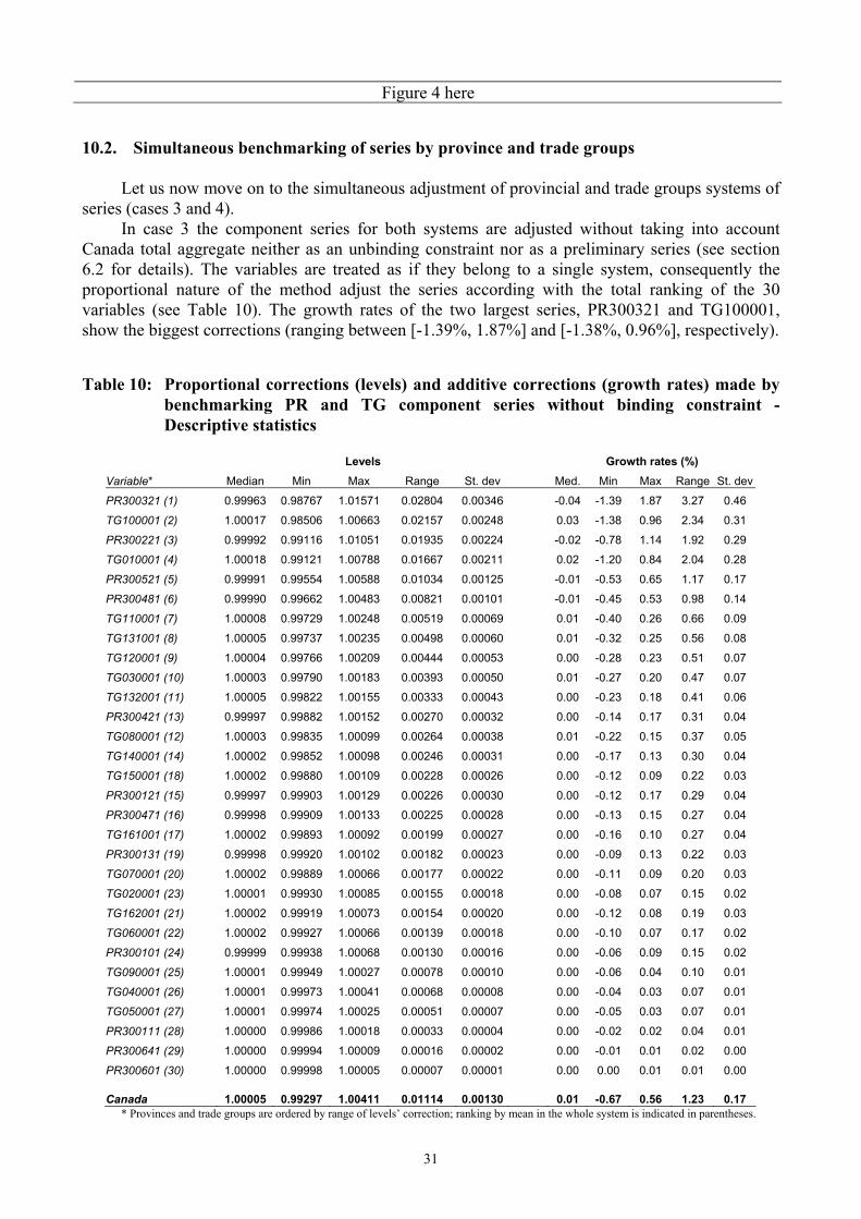
Let us now move on to the simultaneous adjustment of provincial and trade groups systems of series (cases 3 and 4).

In case 3 the component series for both systems are adjusted without taking into account Canada total aggregate neither as an unbinding constraint nor as a preliminary series (see section 6.2 for details). The variables are treated as if they belong to a single system, consequently the proportional nature of the method adjust the series according with the total ranking of the 30 variables (see Table 10). The growth rates of the two largest series, PR300321 and TG100001, show the biggest corrections (ranging between [-1.39%, 1.87%] and [-1.38%, 0.96%], respectively). Table 10: Proportional corrections (levels) and additive corrections (growth rates) made by

benchmarking PR and TG component series without binding constraint - Descriptive statistics

Levels

Growth rates (%) Variable* Median Min Max Range St. dev Med. Min Max Range St. dev

PR300321 (1) 0.99963 0.98767 1.01571 0.02804 0.00346 -0.04 -1.39 1.87 3.27 0.46

TG100001 (2) 1.00017 0.98506 1.00663 0.02157 0.00248 0.03 -1.38 0.96 2.34 0.31

PR300221 (3) 0.99992 0.99116 1.01051 0.01935 0.00224 -0.02 -0.78 1.14 1.92 0.29

TG010001 (4) 1.00018 0.99121 1.00788 0.01667 0.00211 0.02 -1.20 0.84 2.04 0.28

PR300521 (5) 0.99991 0.99554 1.00588 0.01034 0.00125 -0.01 -0.53 0.65 1.17 0.17

PR300481 (6) 0.99990 0.99662 1.00483 0.00821 0.00101 -0.01 -0.45 0.53 0.98 0.14

TG110001 (7) 1.00008 0.99729 1.00248 0.00519 0.00069 0.01 -0.40 0.26 0.66 0.09

TG131001 (8) 1.00005 0.99737 1.00235 0.00498 0.00060 0.01 -0.32 0.25 0.56 0.08

TG120001 (9) 1.00004 0.99766 1.00209 0.00444 0.00053 0.00 -0.28 0.23 0.51 0.07

TG030001 (10) 1.00003 0.99790 1.00183 0.00393 0.00050 0.01 -0.27 0.20 0.47 0.07

TG132001 (11) 1.00005 0.99822 1.00155 0.00333 0.00043 0.00 -0.23 0.18 0.41 0.06

PR300421 (13) 0.99997 0.99882 1.00152 0.00270 0.00032 0.00 -0.14 0.17 0.31 0.04

TG080001 (12) 1.00003 0.99835 1.00099 0.00264 0.00038 0.01 -0.22 0.15 0.37 0.05

TG140001 (14) 1.00002 0.99852 1.00098 0.00246 0.00031 0.00 -0.17 0.13 0.30 0.04

TG150001 (18) 1.00002 0.99880 1.00109 0.00228 0.00026 0.00 -0.12 0.09 0.22 0.03

PR300121 (15) 0.99997 0.99903 1.00129 0.00226 0.00030 0.00 -0.12 0.17 0.29 0.04

PR300471 (16) 0.99998 0.99909 1.00133 0.00225 0.00028 0.00 -0.13 0.15 0.27 0.04

TG161001 (17) 1.00002 0.99893 1.00092 0.00199 0.00027 0.00 -0.16 0.10 0.27 0.04

PR300131 (19) 0.99998 0.99920 1.00102 0.00182 0.00023 0.00 -0.09 0.13 0.22 0.03

TG070001 (20) 1.00002 0.99889 1.00066 0.00177 0.00022 0.00 -0.11 0.09 0.20 0.03

TG020001 (23) 1.00001 0.99930 1.00085 0.00155 0.00018 0.00 -0.08 0.07 0.15 0.02

TG162001 (21) 1.00002 0.99919 1.00073 0.00154 0.00020 0.00 -0.12 0.08 0.19 0.03

TG060001 (22) 1.00002 0.99927 1.00066 0.00139 0.00018 0.00 -0.10 0.07 0.17 0.02

PR300101 (24) 0.99999 0.99938 1.00068 0.00130 0.00016 0.00 -0.06 0.09 0.15 0.02

TG090001 (25) 1.00001 0.99949 1.00027 0.00078 0.00010 0.00 -0.06 0.04 0.10 0.01

TG040001 (26) 1.00001 0.99973 1.00041 0.00068 0.00008 0.00 -0.04 0.03 0.07 0.01

TG050001 (27) 1.00001 0.99974 1.00025 0.00051 0.00007 0.00 -0.05 0.03 0.07 0.01

PR300111 (28) 1.00000 0.99986 1.00018 0.00033 0.00004 0.00 -0.02 0.02 0.04 0.01

PR300641 (29) 1.00000 0.99994 1.00009 0.00016 0.00002 0.00 -0.01 0.01 0.02 0.00

PR300601 (30) 1.00000 0.99998 1.00005 0.00007 0.00001 0.00 0.00 0.01 0.01 0.00

Canada 1.00005 0.99297 1.00411 0.01114 0.00130

0.01 -0.67 0.56 1.23 0.17 * Provinces and trade groups are ordered by range of levels’ correction; ranking by mean in the whole system is indicated in parentheses.

32

As far as TG system is concerned, significant corrections are found only for TG010001, whereas the remaining trade groups remain quite unchanged (see Figure 5). The provincial data show instead greater corrections with respect to the benchmarked figures in case 1 (see Figures 2 and 622). On the contrary, the growth rates of the benchmarked Canada total aggregate are closer to those shown by the preliminary series.

Figure 5 here

Figure 6 here

In case (4) we wish to evaluate whether introducing the Canada preliminary series can induce significant improvements on the benchmarked estimates (Table 11). In fact, the range of corrections is slightly shrunk (from 1.23 to 1.06 for month-to-month rates of change). Furthermore, the whole benchmarked system gets benefit from it (21 out of 30 variables show lower variability of the additive corrections to growth rates, see Figures 7 and 8).

Figure 7 here

Figure 8 here

We display the proportional corrections to the levels (Figure 9) of the unbenchmarked Total Canada series made by the sums of the benchmarked component series in cases (1), (3) and (4), and the additive corrections to month-to-month rates of change (Figure 10) in cases (1) and (3)23. From both graphs it clearly emerges that simultaneous benchmarking of both systems (either with or without a preliminary estimate of the contemporaneous constraint) reduces half of the correction induced by benchmarking system PR only.

Figure 9 here

Figure 10 here

22 It should be noted that the ranges of y-axes in figures 2 and 5 are different. 23 The additive corrections registered in case (4) are practically indistinguishable from those of case (3).

33

Table 11: Proportional corrections (levels) and additive corrections (growth rates) made by simultaneously benchmarking Total Canada, PR and TG component series - Descriptive statistics

Levels

Growth rates (%) Variable* Median Min Max Range St. dev Med. Min Max Range St. dev

PR300321 (1) 0.99961 0.98718 1.01666 0.02948 0.00362 -0.04 -1.47 1.95 3.42 0.48

PR300221 (3) 0.99991 0.99080 1.01114 0.02034 0.00234 -0.03 -0.82 1.19 2.01 0.30

TG100001 (2) 1.00016 0.98629 1.00612 0.01983 0.00229 0.03 -1.27 0.88 2.14 0.28

TG010001 (4) 1.00017 0.99194 1.00727 0.01534 0.00195 0.02 -1.11 0.77 1.88 0.26

PR300521 (5) 0.99990 0.99536 1.00623 0.01087 0.00130 -0.02 -0.56 0.67 1.23 0.17

PR300481 (6) 0.99990 0.99648 1.00512 0.00863 0.00106 -0.01 -0.47 0.55 1.03 0.14

TG110001 (7) 1.00007 0.99752 1.00229 0.00477 0.00064 0.01 -0.37 0.24 0.61 0.09

TG131001 (8) 1.00005 0.99759 1.00217 0.00458 0.00056 0.00 -0.30 0.23 0.52 0.07

TG120001 (9) 1.00004 0.99785 1.00193 0.00408 0.00049 0.00 -0.25 0.21 0.47 0.07

TG030001 (10) 1.00003 0.99808 1.00169 0.00361 0.00046 0.01 -0.25 0.18 0.43 0.06

TG132001 (11) 1.00005 0.99837 1.00143 0.00306 0.00039 0.00 -0.22 0.16 0.38 0.05

PR300421 (13) 0.99997 0.99877 1.00161 0.00284 0.00034 0.00 -0.15 0.18 0.32 0.05

TG080001 (12) 1.00003 0.99849 1.00091 0.00243 0.00035 0.01 -0.20 0.14 0.34 0.05

PR300121 (15) 0.99997 0.99899 1.00137 0.00238 0.00031 0.00 -0.13 0.18 0.30 0.04

PR300471 (16) 0.99998 0.99905 1.00141 0.00236 0.00029 0.00 -0.14 0.15 0.29 0.04

TG140001 (14) 1.00001 0.99864 1.00090 0.00226 0.00029 0.00 -0.16 0.12 0.28 0.04

TG150001 (18) 1.00002 0.99890 1.00100 0.00210 0.00024 0.00 -0.11 0.09 0.20 0.03

PR300131 (19) 0.99998 0.99916 1.00108 0.00191 0.00024 0.00 -0.10 0.13 0.23 0.03

TG161001 (17) 1.00002 0.99901 1.00085 0.00183 0.00025 0.00 -0.15 0.10 0.24 0.03

TG070001 (20) 1.00001 0.99898 1.00061 0.00162 0.00020 0.00 -0.10 0.08 0.19 0.03

TG162001 (21) 0.99998 0.99922 1.00066 0.00145 0.00018 0.00 -0.11 0.07 0.18 0.02

TG020001 (23) 1.00001 0.99936 1.00079 0.00143 0.00017 0.00 -0.08 0.06 0.14 0.02

PR300101 (24) 0.99999 0.99935 1.00072 0.00137 0.00017 0.00 -0.06 0.10 0.16 0.02

TG060001 (22) 1.00002 0.99933 1.00061 0.00128 0.00016 0.00 -0.09 0.06 0.15 0.02

TG090001 (25) 1.00001 0.99953 1.00025 0.00072 0.00009 0.00 -0.06 0.03 0.09 0.01

TG040001 (26) 1.00001 0.99975 1.00038 0.00063 0.00007 0.00 -0.04 0.03 0.06 0.01

PR300641 (29) 0.99965 0.99947 1.00002 0.00055 0.00013 0.00 -0.01 0.01 0.02 0.00

TG050001 (27) 1.00001 0.99976 1.00023 0.00047 0.00007 0.00 -0.04 0.02 0.07 0.01

PR300111 (28) 1.00000 0.99985 1.00019 0.00034 0.00004 0.00 -0.02 0.02 0.04 0.01

PR300601 (30) 1.00000 0.99998 1.00006 0.00008 0.00001 0.00 -0.01 0.01 0.01 0.00

Canada 1.00004 0.99355 1.00380 0.01025 0.00119

0.01 -0.61 0.52 1.13 0.16 * Provinces and trade groups are ordered by range of levels’ correction; ranking by mean in the whole system is indicated in parentheses.

34

Appendix: Derivation of the Moore-Penrose generalized inverse of 'a =Ω HΩH

Denote by a =e He the stochastic disturbances vector obtained by pre-multiplying model (16) by the aggregation matrix H. This vector is characterized by N linear constraints, that is

wwa

wM

= =

H eHe e

WH eH, (A.1)

thus its covariance matrix, ( )' 'a a aE = =e e HΩH Ω , is singular. More precisely, it is:

''

'w w

a ww w

= =

Ω Ω WΩ RΩ R

WΩ WΩ W, (A.2)

where ( )' ''w w w w wE= =Ω H ee H H ΩH is the non-singular covariance matrix of the disturbances

1

w i

M

=

Je

H e Je

Je

.

The Moore-Penrose generalized inverse of aΩ can be built as follows (Powell, 1969, pp. 917-

918): a) select a sub-matrix ( )( )r N r+ × of aΩ , say S, of full column rank r;

b) find a ( )( )r r N× + matrix, say T, such that a =Ω ST ; c) the Moore-Penrose generalized inverse, which is unique, is given by:

( ) ( )1 1' ' ' 'a− −− =Ω T TT S S S . (A.3)

The choice of S and T follows immediately from (A.2):

ww

w

= =

ΩS RΩ

Ω W and [ ]' 'r= =T I W R .

Substitution into (A.3) gives

( ) ( )1 1' ' 'a w w w− −− =Ω R R R Ω R RΩ Ω R ,

from which expression (22) can be easily derived:

( ) ( ) ( ) ( )1 1 1 11 1 1' ' ' ' ' 'a w w w w− − − −− − − −= =Ω R R R Ω R R Ω Ω R R R R Ω R R R .

35

References Barcellan, R. (2002), ECOTRIM: a program for temporal disaggregation of time series, Workshop

on Quarterly National Accounts, Eurostat, Theme 2 Economy and finance: 79-95. Bloem A.M., Dippelsman R.J. and N.Ø. Mæhle (2001), Quarterly National Accounts Manual.

Concepts, Data Sources, and Compilation, International Monetary Fund, Washington DC. Bozik J.E. and M.C. Otto (1988), Benchmarking: Evaluating methods that preserve month-to-

month changes, Bureau of the Census - Statistical Research Division, CENSUS/SRD/RR-88/07.

Chen Z.G. and E.B. Dagum (1997), A recursive method for predicting variables with temporal and

contemporaneous constraints, American Statistical Association, Proceedings of the Business and Economic Statistics Section.

Cholette P.A. (1984), Adjusting sub-annual series to yearly benchmarks, Survey Methodology

10(1): 35-49. Cholette P.A. (1987), Concepts, definitions and principles of benchmarking and interpolation of

time series, Statistics Canada, Time Series Research and Analysis Division, Working Paper No TSRA-87-014E.

Cholette P.A. (1988), Benchmarking systems of socio-economic time series, Statistics Canada, Time

Series Research and Analysis Division, Working Paper No TSRA-88-017E. Cholette P.A. and E.B. Dagum (1994), Benchmarking time series with autocorrelated survey errors,

International Statistical Review 62(3): 365-377. Dagum E.B., Cholette P.A. and Z.G. Chen (1998), A unified view of signal extraction,

benchmarking, interpolation and extrapolation of time series, International Statistical Review 66(3): 245-269.

Denton F.T. (1971), Adjustment of monthly or quarterly series to annual totals: An approach based

on quadratic minimization, Journal of the American Statistical Association, 66(333): 99-102. Di Fonzo T. (2002), Temporal disaggregation of a system of time series when the aggregate is

known. Optimal vs. adjustment methods, Workshop on Quarterly National Accounts, Eurostat, Theme 2 Economy and finance: 63-77.

Durbin J. and B. Quenneville (1997), Benchmarking by state space models, International Statistical

Review 65(1): 23-48. Eurostat (1999), Handbook of quarterly national accounts, Luxembourg, European Commission. Guerrero V.M. and F.H. Nieto (1999), Temporal and contemporaneous disaggregation of multiple

economic time series, Test, 8(2): 459-489. Helfand S.D., Monsour N.J. and M.L. Trager (1977), Historical revision of current business survey

estimates, American Statistical Association, Proceedings of the Business and Economic Statistics Section: 246-250.

36

Hillmer S.C. and A. Trabelsi (1987), Benchmarking of economic time series, Journal of the American Statistical Association, 82(400): 1064-1071.

Laniel N. and K. Fyfe (1989), Benchmarking of economic time series, American Statistical

Association, Proceedings of the Business and Economic Statistics Section: 462-466. Magnus J.R. and H. Neudecker (1988), Matrix differential calculus with applications in statistics

and econometrics, New York, Wiley. Powell A. (1969), Aitken estimator as a tool in allocating predetermined aggregates, Journal of the

American Statistical Association, 64: 913-922. Quilis E.M. (2002), X\TRIMEST. Librería Matlab de procedimientos de desagregacion temporal,

INE (mimeo, available at http://www.ine.es/daco/daco42/daco4214/cbtc29.pdf). Taillon J. (1988), Dessaisonalisation d’un tableau avec contraintes linéaires: Application aux flux

financiers canadiens, The Canadian Journal of Statistics, 16: 97-107.

37

Figure 1: Monthly discrepancies of PR system

-200000

-100000

0

100000

200000

300000

400000

1991 1992 1993 1994 1995 1996 1997 1998 1999 2000

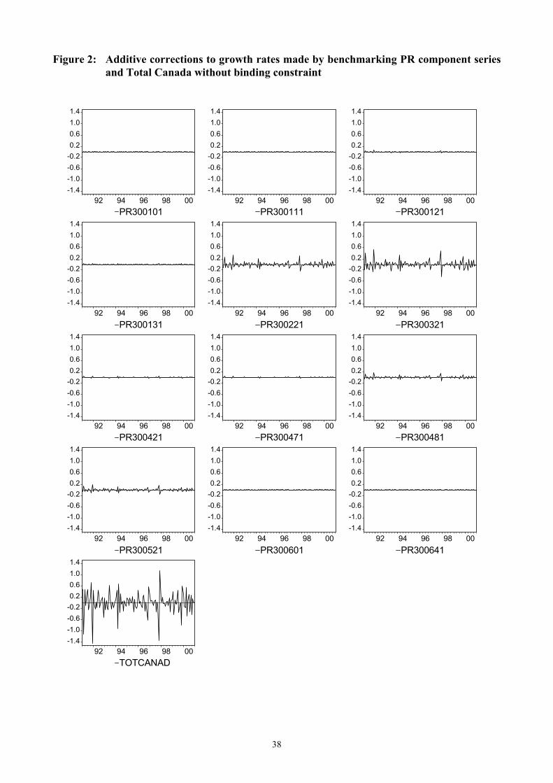
38

Figure 2: Additive corrections to growth rates made by benchmarking PR component series and Total Canada without binding constraint

-1.4-1.0-0.6-0.20.20.61.01.4

92 94 96 98 00PR300101

-1.4-1.0-0.6-0.20.20.61.01.4

92 94 96 98 00PR300111

-1.4-1.0-0.6-0.20.20.61.01.4

92 94 96 98 00PR300121

-1.4-1.0-0.6-0.20.20.61.01.4

92 94 96 98 00PR300131

-1.4-1.0-0.6-0.20.20.61.01.4

92 94 96 98 00PR300221

-1.4-1.0-0.6-0.20.20.61.01.4

92 94 96 98 00PR300321

-1.4-1.0-0.6-0.20.20.61.01.4

92 94 96 98 00PR300421

-1.4-1.0-0.6-0.20.20.61.01.4

92 94 96 98 00PR300471

-1.4-1.0-0.6-0.20.20.61.01.4

92 94 96 98 00PR300481

-1.4-1.0-0.6-0.20.20.61.01.4

92 94 96 98 00PR300521

-1.4-1.0-0.6-0.20.20.61.01.4

92 94 96 98 00PR300601

-1.4-1.0-0.6-0.20.20.61.01.4

92 94 96 98 00PR300641

-1.4-1.0-0.6-0.20.20.61.01.4

92 94 96 98 00TOTCANAD

39

Figure 3: Additive corrections to growth rates made by benchmarking PR component series with a binding constraint

-3.0-2.5-2.0-1.5-1.0-0.50.00.51.01.52.02.53.0

91:01 93:01 95:01 97:01 99:01 01:01

PR300101

-3.0-2.5-2.0-1.5-1.0-0.50.00.51.01.52.02.53.0

91:01 93:01 95:01 97:01 99:01 01:01

PR300111

-3.0-2.5-2.0-1.5-1.0-0.50.00.51.01.52.02.53.0

91:01 93:01 95:01 97:01 99:01 01:01

PR300121

-3.0-2.5-2.0-1.5-1.0-0.50.00.51.01.52.02.53.0

91:01 93:01 95:01 97:01 99:01 01:01

PR300131

-3.0-2.5-2.0-1.5-1.0-0.50.00.51.01.52.02.53.0

91:01 93:01 95:01 97:01 99:01 01:01

PR300221

-3.0-2.5-2.0-1.5-1.0-0.50.00.51.01.52.02.53.0

91:01 93:01 95:01 97:01 99:01 01:01

PR300321

-3.0-2.5-2.0-1.5-1.0-0.50.00.51.01.52.02.53.0

91:01 93:01 95:01 97:01 99:01 01:01

PR300421

-3.0-2.5-2.0-1.5-1.0-0.50.00.51.01.52.02.53.0

91:01 93:01 95:01 97:01 99:01 01:01

PR300471

-3.0-2.5-2.0-1.5-1.0-0.50.00.51.01.52.02.53.0

91:01 93:01 95:01 97:01 99:01 01:01

PR300481

-3.0-2.5-2.0-1.5-1.0-0.50.00.51.01.52.02.53.0

91:01 93:01 95:01 97:01 99:01 01:01

PR300521

-3.0-2.5-2.0-1.5-1.0-0.50.00.51.01.52.02.53.0

91:01 93:01 95:01 97:01 99:01 01:01

PR300601

-3.0-2.5-2.0-1.5-1.0-0.50.00.51.01.52.02.53.0

91:01 93:01 95:01 97:01 99:01 01:01

PR300641

40

Figure 4: Additive corrections to growth rates made by benchmarking PR component series while preserving the growth rates and with binding constraint

-3.0

-2.0

-1.0

0.0

1.0

2.0

3.0

92 94 96 98 00PR300101

-3.0

-2.0

-1.0

0.0

1.0

2.0

3.0

92 94 96 98 00PR300111

-3.0

-2.0

-1.0

0.0

1.0

2.0

3.0

92 94 96 98 00PR300121

-3.0

-2.0

-1.0

0.0

1.0

2.0

3.0

92 94 96 98 00PR300131

-3.0

-2.0

-1.0

0.0

1.0

2.0

3.0

92 94 96 98 00PR300221

-3.0

-2.0

-1.0

0.0

1.0

2.0

3.0

92 94 96 98 00PR300321

-3.0

-2.0

-1.0

0.0

1.0

2.0

3.0

92 94 96 98 00PR300421

-3.0

-2.0

-1.0

0.0

1.0

2.0

3.0

92 94 96 98 00PR300471

-3.0

-2.0

-1.0

0.0

1.0

2.0

3.0

92 94 96 98 00PR300481

-3.0

-2.0

-1.0

0.0

1.0

2.0

3.0

92 94 96 98 00PR300521

-3.0

-2.0

-1.0

0.0

1.0

2.0

3.0

92 94 96 98 00PR300601

-3.0

-2.0

-1.0

0.0

1.0

2.0

3.0

92 94 96 98 00PR300641

41

Figure 5: Additive corrections to growth rates made by benchmarking PR and TG component series without a binding constraint – Series by trade groups

-1.4

-1.0

-0.6

-0.2

0.2

0.6

1.0

1.4

1992 1994 1996 1998 2000

TG010001

-1.4

-1.0

-0.6

-0.2

0.2

0.6

1.0

1.4

1992 1994 1996 1998 2000

TG020001

-1.4

-1.0

-0.6

-0.2

0.2

0.6

1.0

1.4

1992 1994 1996 1998 2000

TG030001

-1.4

-1.0

-0.6

-0.2

0.2

0.6

1.0

1.4

1992 1994 1996 1998 2000

TG040001

-1.4

-1.0

-0.6

-0.2

0.2

0.6

1.0

1.4

1992 1994 1996 1998 2000

TG050001

-1.4

-1.0

-0.6

-0.2

0.2

0.6

1.0

1.4

1992 1994 1996 1998 2000

TG060001

-1.4

-1.0

-0.6

-0.2

0.2

0.6

1.0

1.4

1992 1994 1996 1998 2000

TG070001

-1.4

-1.0

-0.6

-0.2

0.2

0.6

1.0

1.4

1992 1994 1996 1998 2000

TG080001

-1.4

-1.0

-0.6

-0.2

0.2

0.6

1.0

1.4

1992 1994 1996 1998 2000

TG090001

-1.4

-1.0

-0.6

-0.2

0.2

0.6

1.0

1.4

1992 1994 1996 1998 2000

TG100001

-1.4

-1.0

-0.6

-0.2

0.2

0.6

1.0

1.4

1992 1994 1996 1998 2000

TG110001

-1.4

-1.0

-0.6

-0.2

0.2

0.6

1.0

1.4

1992 1994 1996 1998 2000

TG120001

-1.4

-1.0

-0.6

-0.2

0.2

0.6

1.0

1.4

1992 1994 1996 1998 2000

TG131001

-1.4

-1.0

-0.6

-0.2

0.2

0.6

1.0

1.4

1992 1994 1996 1998 2000

TG132001

-1.4

-1.0

-0.6

-0.2

0.2

0.6

1.0

1.4

1992 1994 1996 1998 2000

TG140001

-1.4

-1.0

-0.6

-0.2

0.2

0.6

1.0

1.4

1992 1994 1996 1998 2000

TG150001

-1.4

-1.0

-0.6

-0.2

0.2

0.6

1.0

1.4

1992 1994 1996 1998 2000

TG161001

-1.4

-1.0

-0.6

-0.2

0.2

0.6

1.0

1.4

1992 1994 1996 1998 2000

TG162001

42

Figure 6: Additive corrections to growth rates made by benchmarking PR and TG component series without a binding constraint – Series by province and Total Canada

-2.0-1.6-1.2-0.8-0.40.00.40.81.21.62.0

1992 1994 1996 1998 2000

PR300101

-2.0-1.6-1.2-0.8-0.40.00.40.81.21.62.0

1992 1994 1996 1998 2000

PR300111

-2.0-1.6-1.2-0.8-0.40.00.40.81.21.62.0

1992 1994 1996 1998 2000

PR300121

-2.0-1.6-1.2-0.8-0.40.00.40.81.21.62.0

1992 1994 1996 1998 2000

PR300131

-2.0-1.6-1.2-0.8-0.40.00.40.81.21.62.0

1992 1994 1996 1998 2000

PR300221

-2.0-1.6-1.2-0.8-0.40.00.40.81.21.62.0

1992 1994 1996 1998 2000

PR300321

-2.0-1.6-1.2-0.8-0.40.00.40.81.21.62.0

1992 1994 1996 1998 2000

PR300421

-2.0-1.6-1.2-0.8-0.40.00.40.81.21.62.0

1992 1994 1996 1998 2000

PR300471

-2.0-1.6-1.2-0.8-0.40.00.40.81.21.62.0

1992 1994 1996 1998 2000

PR300481

-2.0-1.6-1.2-0.8-0.40.00.40.81.21.62.0

1992 1994 1996 1998 2000

PR300521

-2.0-1.6-1.2-0.8-0.40.00.40.81.21.62.0

1992 1994 1996 1998 2000

PR300601

-2.0-1.6-1.2-0.8-0.40.00.40.81.21.62.0

1992 1994 1996 1998 2000

PR300641

-2.0-1.6-1.2-0.8-0.40.00.40.81.21.62.0

1992 1994 1996 1998 2000

TOTCANAD

43

Figure 7: Additive corrections to growth rates made by benchmarking Total Canada, PR and TG component series - Series by trade groups

-1.4

-1.0

-0.6

-0.2

0.2

0.6

1.0

1.4

1992 1994 1996 1998 2000

TG010001

-1.4

-1.0

-0.6

-0.2

0.2

0.6

1.0

1.4

1992 1994 1996 1998 2000

TG020001

-1.4

-1.0

-0.6

-0.2

0.2

0.6

1.0

1.4

1992 1994 1996 1998 2000

TG030001

-1.4

-1.0

-0.6

-0.2

0.2

0.6

1.0

1.4

1992 1994 1996 1998 2000

TG040001

-1.4

-1.0

-0.6

-0.2

0.2

0.6

1.0

1.4

1992 1994 1996 1998 2000

TG050001

-1.4

-1.0

-0.6

-0.2

0.2

0.6

1.0

1.4

1992 1994 1996 1998 2000

TG060001

-1.4

-1.0

-0.6

-0.2

0.2

0.6

1.0

1.4

1992 1994 1996 1998 2000

TG070001

-1.4

-1.0

-0.6

-0.2

0.2

0.6

1.0

1.4

1992 1994 1996 1998 2000

TG080001

-1.4

-1.0

-0.6

-0.2

0.2

0.6

1.0

1.4

1992 1994 1996 1998 2000

TG090001

-1.4

-1.0

-0.6

-0.2

0.2

0.6

1.0

1.4

1992 1994 1996 1998 2000

TG100001

-1.4

-1.0

-0.6

-0.2

0.2

0.6

1.0

1.4

1992 1994 1996 1998 2000

TG110001

-1.4

-1.0

-0.6

-0.2

0.2

0.6

1.0

1.4

1992 1994 1996 1998 2000

TG120001

-1.4

-1.0

-0.6

-0.2

0.2

0.6

1.0

1.4

1992 1994 1996 1998 2000

TG131001

-1.4

-1.0

-0.6

-0.2

0.2

0.6

1.0

1.4

1992 1994 1996 1998 2000

TG132001

-1.4

-1.0

-0.6

-0.2

0.2

0.6

1.0

1.4

1992 1994 1996 1998 2000

TG140001

-1.4

-1.0

-0.6

-0.2

0.2

0.6

1.0

1.4

1992 1994 1996 1998 2000

TG150001

-1.4

-1.0

-0.6

-0.2

0.2

0.6

1.0

1.4

1992 1994 1996 1998 2000

TG161001

-1.4

-1.0

-0.6

-0.2

0.2

0.6

1.0

1.4

1992 1994 1996 1998 2000

TG162001

44

Figure 8: Additive corrections to growth rates made by benchmarking Total Canada, PR and TG component series - Series by province and Total Canada

-2.5-2.0-1.5-1.0-0.50.00.51.01.52.02.5

1992 1994 1996 1998 2000

PR300101

-2.5-2.0-1.5-1.0-0.50.00.51.01.52.02.5

1992 1994 1996 1998 2000

PR300111

-2.5-2.0-1.5-1.0-0.50.00.51.01.52.02.5

1992 1994 1996 1998 2000

PR300121

-2.5-2.0-1.5-1.0-0.50.00.51.01.52.02.5

1992 1994 1996 1998 2000

PR300131

-2.5-2.0-1.5-1.0-0.50.00.51.01.52.02.5

1992 1994 1996 1998 2000

PR300221

-2.5-2.0-1.5-1.0-0.50.00.51.01.52.02.5

1992 1994 1996 1998 2000

PR300321

-2.5-2.0-1.5-1.0-0.50.00.51.01.52.02.5

1992 1994 1996 1998 2000

PR300421

-2.5-2.0-1.5-1.0-0.50.00.51.01.52.02.5

1992 1994 1996 1998 2000

PR300471

-2.5-2.0-1.5-1.0-0.50.00.51.01.52.02.5

1992 1994 1996 1998 2000

PR300481

-2.5-2.0-1.5-1.0-0.50.00.51.01.52.02.5

1992 1994 1996 1998 2000

PR300521

-2.5-2.0-1.5-1.0-0.50.00.51.01.52.02.5

1992 1994 1996 1998 2000

PR300601

-2.5-2.0-1.5-1.0-0.50.00.51.01.52.02.5

1992 1994 1996 1998 2000

PR300641

-2.5-2.0-1.5-1.0-0.50.00.51.01.52.02.5

1992 1994 1996 1998 2000

TOTCANAD

45

Figure 9: Proportional corrections to the unbenchmarked SA Total Canada made by the sum of variously benchmarked SA series

0.985

0.990

0.995

1.000

1.005

1.010

1991 1992 1993 1994 1995 1996 1997 1998 1999 2000

PR PRTG PRTGP

* PR: case 1; PRTG: case 3; PRTGP: case 4. Figure 10: Additive corrections to rates of change of unbenchmarked SA Total Canada series

made by the sum of variously benchmarked SA series

-1.6

-1.2

-0.8

-0.4

0.0

0.4

0.8

1.2

1991 1992 1993 1994 1995 1996 1997 1998 1999 2000

PR PRTG

* PR: case 1; PRTG: case 3.