Benchmarking Replication in NoSQL Data Stores · Benchmarking Replication in NoSQL Data Stores by Gerard Haughian ... As such this study paves the way for a new replication benchmarking

Imperial College London

Department of Computing

Benchmarking Replication in NoSQL DataStores

by

Gerard Haughian (gh413)

Submitted in partial fulfilment of the requirements for the MSc Degree in Computing Science ofImperial College London

September 2014

Abstract

The proliferation in Web 2.0 applications has increased both the volume, velocity, and va-riety of data sources which have exceeded the limitations and expected use cases of traditionalrelational DBMSs. Cloud serving NoSQL data stores address these concerns and provide replica-tion mechanisms to ensure fault tolerance, high availability, and improved scalability. However,no research or studies exist which emperically explore the impact of replication on data storeperformance.

As such this study paves the way for a new replication benchmarking tier for YCSB, a leadingbenchmark tool for cloud serving data stores, by benchmarking replication in four NoSQL datastores of variable categorization and replication strategy. These data stores include: Redis, a key-value store that uses a master-slave replication model; MongoDB, a document store with replicaset replication; Cassandra, an extensible-record store with a multi-master replica architecture;and VoltDB, a distributed DBMS which utilizes a synchronous multi-master replication strategy.This study focuses on the impact of replication on performance and availability compared tonon-replicated clusters on constant amounts of hardware. To increase the relevancy of thisstudy to real-world use cases, experiments include different workloads, distributions, and tunableconsistency levels, on clusters hosted on a private cloud environment.

This study presents an in-depth analysis of the overall throughput, read latencies, and writelatencies of all experiments per data store. Each analysis section concludes with a presentationand brief analysis of the latency histogram and CDF curves of reads and writes to aid predictionson how each data store should behave. Subsequently, a comparative analysis is performedbetween data stores to identify the most performant data store and replication model.

This study should serve as a point of reference for companies attempting to choose the rightdata store and replication strategy for their use cases. It also highlights the need to investigatethe effects of geo-replication in more detail due to its importance in ensuring high availability inthe face of network partitions and data center failures. Additionally, the impact that replicationhas on the consistency of data is of importance and warrants further attention. By making thedata collected in this study publicly available, we encourage further research in an area withconsiderable research gaps: performance modelling of NoSQL data stores.

2

Acknowledgements

A special thanks to my supervisor, Rasha Osman, for her unyielding support and enthusiasmfor this work and her fantastic guidance throughout.

Dedication

To Paddy, Una, Luke, Eamon, and Ewa who, as always, have proven the rock that bonds usremains so pure and unbreakable. With their belief and understanding, much has been and willcontinue to be achieved. Thanks for never giving up on me.

3

Contents

1 Introduction 81.1 Aims and Objectives . . . . . . . . . . . . . . . . . . . . . . . . . . . . . . . . . . 91.2 Contributions . . . . . . . . . . . . . . . . . . . . . . . . . . . . . . . . . . . . . . 91.3 Report Outline . . . . . . . . . . . . . . . . . . . . . . . . . . . . . . . . . . . . . 10

2 Related Work 112.1 Benchmarking Tools . . . . . . . . . . . . . . . . . . . . . . . . . . . . . . . . . . 11

2.1.1 Benchmarking Traditional Systems . . . . . . . . . . . . . . . . . . . . . . 112.1.2 Benchmarking NoSQL Systems . . . . . . . . . . . . . . . . . . . . . . . . 12

2.2 Academic YCSB Benchmarking Studies . . . . . . . . . . . . . . . . . . . . . . . 132.3 Industry YCSB Benchmarking Studies . . . . . . . . . . . . . . . . . . . . . . . . 142.4 Extended YCSB Benchmarking Studies . . . . . . . . . . . . . . . . . . . . . . . 152.5 Additional Studies . . . . . . . . . . . . . . . . . . . . . . . . . . . . . . . . . . . 152.6 Summary . . . . . . . . . . . . . . . . . . . . . . . . . . . . . . . . . . . . . . . . 16

3 Systems Under Investigation 173.1 Redis . . . . . . . . . . . . . . . . . . . . . . . . . . . . . . . . . . . . . . . . . . . 173.2 MongoDB . . . . . . . . . . . . . . . . . . . . . . . . . . . . . . . . . . . . . . . . 183.3 Cassandra . . . . . . . . . . . . . . . . . . . . . . . . . . . . . . . . . . . . . . . . 193.4 VoltDB . . . . . . . . . . . . . . . . . . . . . . . . . . . . . . . . . . . . . . . . . 21

4 Experimental Setup 234.1 YCSB Configuration . . . . . . . . . . . . . . . . . . . . . . . . . . . . . . . . . . 23

4.1.1 Warm-up Extension . . . . . . . . . . . . . . . . . . . . . . . . . . . . . . 244.2 Data Store Configuration and Optimization . . . . . . . . . . . . . . . . . . . . . 24

4.2.1 Redis . . . . . . . . . . . . . . . . . . . . . . . . . . . . . . . . . . . . . . 254.2.2 MongoDB . . . . . . . . . . . . . . . . . . . . . . . . . . . . . . . . . . . . 254.2.3 Cassandra . . . . . . . . . . . . . . . . . . . . . . . . . . . . . . . . . . . . 264.2.4 VoltDB . . . . . . . . . . . . . . . . . . . . . . . . . . . . . . . . . . . . . 26

4.3 Methodology . . . . . . . . . . . . . . . . . . . . . . . . . . . . . . . . . . . . . . 27

5 Experimental Results 295.1 Redis . . . . . . . . . . . . . . . . . . . . . . . . . . . . . . . . . . . . . . . . . . . 295.2 MongoDB . . . . . . . . . . . . . . . . . . . . . . . . . . . . . . . . . . . . . . . . 365.3 Cassandra . . . . . . . . . . . . . . . . . . . . . . . . . . . . . . . . . . . . . . . . 435.4 VoltDB . . . . . . . . . . . . . . . . . . . . . . . . . . . . . . . . . . . . . . . . . 515.5 Comparative Analysis . . . . . . . . . . . . . . . . . . . . . . . . . . . . . . . . . 57

6 Conclusion 606.1 Benchmarking Results . . . . . . . . . . . . . . . . . . . . . . . . . . . . . . . . . 606.2 Limitations . . . . . . . . . . . . . . . . . . . . . . . . . . . . . . . . . . . . . . . 616.3 Future Work . . . . . . . . . . . . . . . . . . . . . . . . . . . . . . . . . . . . . . 62

A Extended Redis Client YCSB code 66

B Extended MongoDB Client YCSB code 68

C System Monitoring: Ganglia Configuration and Setup 70

4

List of Tables

3.1 NoSQL Data Store Choices by Category, and Replication Strategy. . . . . . . . . 174.1 Virtual Machine Specifications and Settings. . . . . . . . . . . . . . . . . . . . . . 234.2 Optimal Warm-up Times For Each Data Store. . . . . . . . . . . . . . . . . . . . 244.3 Redis Configuration Settings. . . . . . . . . . . . . . . . . . . . . . . . . . . . . . 254.4 Complete List of Experiments. . . . . . . . . . . . . . . . . . . . . . . . . . . . . 275.1 Redis: Percentage Differences In Read & Write Latencies and Overall Throughput

Between Distributions for each Workload and Consistency Level. . . . . . . . . . 325.2 Redis: Read & Write Latency and Overall Throughput & 95th% Confidence

Interval Data per Workload, Broken Down by Distribution and Consistency Level. 325.3 Redis: Percentage Differences In Read & Write Latencies and Overall Throughput

Between Workloads for each Distribution and Consistency Level. . . . . . . . . . 335.4 MongoDB: Percentage Differences In Read & Write Latencies and Overall Through-

put Between Workloads for each Distribution and Consistency Level. . . . . . . . 365.5 MongoDB: Read & Write Latency & 95th Percentiles and Overall Throughput

& 95th% Confidence Interval Data per Workload, Broken Down by Distributionand Consistency Level. . . . . . . . . . . . . . . . . . . . . . . . . . . . . . . . . . 39

5.6 MongoDB: Percentage Differences in Read & Write Latencies and Overall Through-put From Baseline Experiments per Workload, Broken Down by Distribution andConsistency Level. . . . . . . . . . . . . . . . . . . . . . . . . . . . . . . . . . . . 40

5.7 MongoDB: Percentage Differences In Read & Write Latencies and Overall Through-put Between Distributions for each Workload and Consistency Level. . . . . . . . 40

5.8 Cassandra: Read & Write Latency & 95th Percentiles and Overall Throughput& 95th% Confidence Interval Data per Workload, Broken Down by Distributionand Consistency Level. . . . . . . . . . . . . . . . . . . . . . . . . . . . . . . . . . 46

5.9 Cassandra: Percentage Differences In Read & Write Latencies and Overall Through-put Between Distributions for each Workload and Consistency Level. . . . . . . . 47

5.10 Cassandra: Percentage Differences in Read & Write Latencies and Overall Through-put From Baseline Experiments per Workload, Broken Down by Distribution andConsistency Level. . . . . . . . . . . . . . . . . . . . . . . . . . . . . . . . . . . . 47

5.11 Cassandra: Percentage Differences In Read & Write Latencies and Overall Through-put Between Workloads for each Distribution and Consistency Level. . . . . . . . 48

5.12 VoltDB: Percentage Differences in Read & Write Latencies and Overall Through-put From Baseline Experiments per Workload, Broken Down by Distribution. . . 52

5.13 VoltDB: Percentage of Workload Reads Impact on Read Latency and OverallThroughput. . . . . . . . . . . . . . . . . . . . . . . . . . . . . . . . . . . . . . . 53

5.14 VoltDB: Percentage Differences In Read & Write Latencies and Overall Through-put Between Workloads for each Distribution. . . . . . . . . . . . . . . . . . . . . 54

5.15 VoltDB: Overall Throughput Differences Between No-Replication and No-Replicationor Command Logging Experiments. . . . . . . . . . . . . . . . . . . . . . . . . . . 55

5.16 VoltDB: Percentage Differences In Read & Write Latencies and Overall Through-put Between Distributions for each Workload. . . . . . . . . . . . . . . . . . . . . 55

5.17 VoltDB: Read & Write Latency & 95th Percentiles and Overall Throughput &95th% Confidence Interval Data per Workload, Broken Down by Distribution. . . 55

5

List of Figures

3.1 Redis Architecture. . . . . . . . . . . . . . . . . . . . . . . . . . . . . . . . . . . . 183.2 MongoDB Architecture. . . . . . . . . . . . . . . . . . . . . . . . . . . . . . . . . 193.3 Cassandra Architecture. . . . . . . . . . . . . . . . . . . . . . . . . . . . . . . . . 203.4 VoltDB Architecture. . . . . . . . . . . . . . . . . . . . . . . . . . . . . . . . . . . 224.1 VoltDB Warm-up Illustration. . . . . . . . . . . . . . . . . . . . . . . . . . . . . . 245.1 Redis: Overall Throughputs per Consistency Level for all Workloads and Distri-

butions: (a) ONE (b) QUORUM (c) ALL. . . . . . . . . . . . . . . . . . . . . . . 305.2 Redis: Read Latencies per Consistency Level for all Workloads and Distributions:

(a) ONE (b) QUORUM (c) ALL. . . . . . . . . . . . . . . . . . . . . . . . . . . . 305.3 Redis: Write Latencies per Consistency Level for all Workloads and Distributions:

(a) ONE (b) QUORUM (c) ALL. . . . . . . . . . . . . . . . . . . . . . . . . . . . 315.4 Redis Workload G Read Latency Histograms: (a) Uniform ONE (b) Uniform

QUORUM (c) Uniform ALL (d) Zipfian ONE (e) Zipfian QUORUM (f) ZipfianALL (g) Latest ONE (h) Latest QUORUM (i) Latest ALL. . . . . . . . . . . . . 33

5.5 Redis Workload G Write Latency Histograms: (a) Uniform ONE (b) UniformQUORUM (c) Uniform ALL (d) Zipfian ONE (e) Zipfian QUORUM (f) ZipfianALL (g) Latest ONE (h) Latest QUORUM (i) Latest ALL. . . . . . . . . . . . . 34

5.6 Redis Workload H Read Latency Histograms: (a) Uniform ONE (b) UniformQUORUM (c) Uniform ALL (d) Zipfian ONE (e) Zipfian QUORUM (f) ZipfianALL (g) Latest ONE (h) Latest QUORUM (i) Latest ALL. . . . . . . . . . . . . 34

5.7 Redis Workload H Write Latency Histograms: (a) Uniform ONE (b) UniformQUORUM (c) Uniform ALL (d) Zipfian ONE (e) Zipfian QUORUM (f) ZipfianALL (g) Latest ONE (h) Latest QUORUM (i) Latest ALL. . . . . . . . . . . . . 35

5.8 MongoDB: Overall Throughputs per Consistency Level for all Workloads andDistributions: (a) ONE (b) QUORUM (c) ALL. . . . . . . . . . . . . . . . . . . 37

5.9 MongoDB: Read Latencies per Consistency Level for all Workloads and Distri-butions: (a) ONE (b) QUORUM (c) ALL. . . . . . . . . . . . . . . . . . . . . . . 38

5.10 MongoDB: Write Latencies per Consistency Level for all Workloads and Distri-butions: (a) ONE (b) QUORUM (c) ALL. . . . . . . . . . . . . . . . . . . . . . . 38

5.11 MongoDB Workload G Read Latency Histograms: (a) Uniform ONE (b) UniformQUORUM (c) Uniform ALL (d) Zipfian ONE (e) Zipfian QUORUM (f) ZipfianALL (g) Latest ONE (h) Latest QUORUM (i) Latest ALL. . . . . . . . . . . . . 41

5.12 MongoDB Workload G Write Latency Histograms: (a) Uniform ONE (b) UniformQUORUM (c) Uniform ALL (d) Zipfian ONE (e) Zipfian QUORUM (f) ZipfianALL (g) Latest ONE (h) Latest QUORUM (i) Latest ALL. . . . . . . . . . . . . 41

5.13 MongoDB Workload H Read Latency Histograms: (a) Uniform ONE (b) UniformQUORUM (c) Uniform ALL (d) Zipfian ONE (e) Zipfian QUORUM (f) ZipfianALL (g) Latest ONE (h) Latest QUORUM (i) Latest ALL. . . . . . . . . . . . . 42

5.14 MongoDB Workload H Write Latency Histograms: (a) Uniform ONE (b) UniformQUORUM (c) Uniform ALL (d) Zipfian ONE (e) Zipfian QUORUM (f) ZipfianALL (g) Latest ONE (h) Latest QUORUM (i) Latest ALL. . . . . . . . . . . . . 42

5.15 Cassandra: Overall Throughputs per Consistency Level for all Workloads andDistributions: (a) ONE (b) QUORUM (c) ALL. . . . . . . . . . . . . . . . . . . 43

5.16 Cassandra: Read Latencies per Consistency Level for all Workloads and Distri-butions: (a) ONE (b) QUORUM (c) ALL. . . . . . . . . . . . . . . . . . . . . . . 44

5.17 Cassandra: Write Latencies per Consistency Level for all Workloads and Distri-butions: (a) ONE (b) QUORUM (c) ALL. . . . . . . . . . . . . . . . . . . . . . . 44

5.18 Cassandra Workload G Read Latency Histograms: (a) Uniform ONE (b) UniformQUORUM (c) Uniform ALL (d) Zipfian ONE (e) Zipfian QUORUM (f) ZipfianALL (g) Latest ONE (h) Latest QUORUM (i) Latest ALL. . . . . . . . . . . . . 48

5.19 Cassandra Workload G Write Latency Histograms: (a) Uniform ONE (b) UniformQUORUM (c) Uniform ALL (d) Zipfian ONE (e) Zipfian QUORUM (f) ZipfianALL (g) Latest ONE (h) Latest QUORUM (i) Latest ALL. . . . . . . . . . . . . 49

5.20 Cassandra Workload H Read Latency Histograms: (a) Uniform ONE (b) UniformQUORUM (c) Uniform ALL (d) Zipfian ONE (e) Zipfian QUORUM (f) ZipfianALL (g) Latest ONE (h) Latest QUORUM (i) Latest ALL. . . . . . . . . . . . . 49

5.21 Cassandra Workload H Write Latency Histograms: (a) Uniform ONE (b) UniformQUORUM (c) Uniform ALL (d) Zipfian ONE (e) Zipfian QUORUM (f) ZipfianALL (g) Latest ONE (h) Latest QUORUM (i) Latest ALL. . . . . . . . . . . . . 50

6

5.22 VoltDB: Overall Throughput per Distribution: (a) Workload G (b) Workload H. 515.23 VoltDB: Read Latencies per Distribution: (a) Workload G (b) Workload H. . . . 515.24 VoltDB: Write Latencies per Distribution: (a) Workload G (b) Workload H. . . . 525.25 VoltDB: Combined Performance Metrics for each Workload and Distribution: (a)

Throughputs (b) Read Latencies (c) Write Latencies. . . . . . . . . . . . . . . . . 545.26 VoltDB Overall Throughputs per Distribution and Baseline Experiments with no

Command Logging: (a) Workload G (b) Workload H. . . . . . . . . . . . . . . . 545.27 VoltDB Workload G Read Latency Histograms: (a) Uniform (b) Zipfian (c) Latest. 565.28 VoltDB Workload G Write Latency Histograms: (a) Uniform (b) Zipfian (c) Latest. 565.29 VoltDB Workload H Read Latency Histograms: (a) Uniform (b) Zipfian (c) Latest. 565.30 VoltDB Workload H Write Latency Histograms: (a) Uniform (b) Zipfian (c) Latest. 565.31 Comparison of Data Stores averaged across all distributions and consistency levels

for Workload G: (a) Overall Throughput (b) Read Latency (c) Write Latency. . . 575.32 Comparison of Data Stores averaged across all distributions and consistency levels

for Workload H: (a) Overall Throughput (b) Read Latency (c) Write Latency. . . 585.33 Comparison of Replication strategies: Multi-Master (Cassandra) and Replica Sets

(MongoDB), averaged across all distributions and consistency levels for WorkloadG: (a) Overall Throughput (b) Read Latency (c) Write Latency. . . . . . . . . . 59

5.34 Comparison of Replication strategies: Multi-Master (Cassandra) and Replica Sets(MongoDB), averaged across all distributions and consistency levels for WorkloadH: (a) Overall Throughput (b) Read Latency (c) Write Latency. . . . . . . . . . 59

C.1 Ganglia Architecture. . . . . . . . . . . . . . . . . . . . . . . . . . . . . . . . . . 70C.2 Example Ganglia Web Interface. . . . . . . . . . . . . . . . . . . . . . . . . . . . 71

7

1 Introduction

Traditional relational database systems of the 1970s were designed to suit the requirementsof On-line Transactional Processing (OLTP) applications as “one-size-fits-all” solutions [69].These systems are typically hosted on a single server, where database administrators respondto increases in data set sizes by increasing the CPU compute power, the amount of availablememory, and the speed of hard disks on that single server, i.e., by scaling vertically. Relationaldatabase systems still remain relevant in today’s modern computing environment, however thelimitations of vertical scalability is of greatest concern.

The volume of data consumed by many organizations in recent years has now considerablyoutgrown the capacity of a single server, due to the explosion of the web [32]. Therefore, newtechnologies and techniques had to be developed to address what has become known as the BigData era. In 2010, it was claimed that Facebook hosted the world’s largest data warehousehosted on HDFS (Hadoop’s distributed file system), comprising 2000 servers, consuming 21Petabyte’s (PB) of storage [7], which rapidly grew to 100 PB as early as 2012 [62].

This situation is further complicated by the fact that traditional OLTP applications remainonly a subset of the use cases that these new technologies must facilitate, proliferated by adiverse range of modern industry application requirements [14]. Subsequently, Big Data tech-nologies are required to scale in a new way to overcome the limitations of a single server’s CPUcompute power, memory capacity, and disk I/O speeds. Horizontal scalability has thereforebecome the new focus for data store systems; offering the ability to spread data across and servedata from multiple servers.

Elasticity is a property of horizontal scalability, which enables linear increases in throughputas more machines are added to a cluster1. The modern computing environment has also seenan increase in the number of cloud computing service providers. Many of which are inherentlyelastic, for example Amazon’s AWS [64] and Rackspace [57], which provide horizontal scalabilitywith ease and at low cost to the user2.

Many new data stores have been designed with this change of landscape in mind; some ofwhich have even been designed to work exclusively in the cloud, for example Yahoo’s PNUTS[13], Google’s BigTable [11], and Amazon’s DynamoDB [66]. These new data store systems arecommonly referred to as NoSQL data stores, which stands for “Not Only SQL”; since they donot use the Structured Query Language (SQL)3, or have a relational model4. Hewitt [32] furthersuggests that this term also means that traditional systems should not be the only choice fordata storage.

There exists a vast array of NoSQL data store solutions, and companies that turn to thesesolutions to contend with the challenges of data scalability, are faced with the initial challengeof choosing the best one for their particular use case. The data which companies gather andcollect is highly valuable and access to this data often needs to be highly available [27]. The needfor high availability of data becomes particularly evident in the Web 2.05 applications which weourselves may have become accustomed to interacting with on a daily basis, for example socialmedia platforms like Facebook and Twitter.

A feature of horizontal scalability is the lower grade of servers which form a cluster. Theseservers are typically commodity hardware which have inherently higher failure rates due to theircheaper components. A larger number of servers also increases the frequency of experiencinga node failure. The primary mechanism in which NoSQL data stores offer high availability inorder to overcome a higher rate of failure and meet industry expectations is through replication.

1Throughout this report, the term “cluster” refers to a collection of servers or nodes connected together with aknown topology, operating as a distributed data store system.

2On Amazon’s S3 service, the cost of storing 1 GB of data is only $0.125. For more detail see: http://docs.

aws.amazon.com/gettingstarted/latest/wah/web-app-hosting-pricing-s3.html Last Accessed: 2014.07.073SQL is a feature-rich and simple declarative language for defining and manipulating data in traditional relational

database systems.4The relational model is a database model based on first order logic, were all data is represented as tuples and

grouped into relations. Databases organized in this way are referred to as relational databases.5Web 2.0 as described by O’Reilly [50] : “Web 2.0 is the network as [a] platform [. . . ]; Web 2.0 applications are

those that make the most of the intrinsic advantages of that platform: delivering software as a continually-updatedservice that gets better the more people use it, consuming and remixing data from multiple sources, [. . . ], creatingnetwork effects through an ‘architecture of participation’, and going beyond the page metaphor of Web 1.0 to deliverrich user experiences.”.

8

Replication not only offers higher redundancy in the event of failure but can also help avoiddata loss (by recovering lost data from a replica), and improve performance (by spreading loadacross multiple replicas) [14].

1.1 Aims and Objectives

The aims and objectives of this study are:

• Offer insights based on the quantitative analysis of benchmarking results on the impactreplication has on four different NoSQL data stores of variable categorization and replica-tion model.

• Illustrate the impact replication has on performance and availability of cloud servingNoSQL data stores on various cluster sizes relative to non-replicated clusters of equalsizes.

• Evalute, through the application of both read- and write-heavy workloads the impact ofeach data stores underlying optimizations and design decisions within replicated clusters.

• Explore the impact on performance within replicated clusters of three varying (in termsof strictness) levels of tunable consistency including ONE, QUORUM6, and ALL.

• Construct a more comprehensive insight into each data store’s suitability to different indus-try applications by experimenting with three different data distributions, each simulatinga different real-world use case.

• Help alleviate the challenges faced by companies and individuals choosing an appropriatedata store to meet their scalability and fault-tolerance needs.

• Provide histograms and CDF curves as a starting point for future research into perfor-mance modeling of NoSQL data stores.

1.2 Contributions

This study extends the work of Cooper et al. [14] who created a benchmarking tool (YCSB)specifically for cloud serving NoSQL data stores. Cooper et al. highlighted four important mea-sures required for adding a fourth tier to their YCSB tool for benchmarking replication. Thosefour measures were: performance cost and benefit; availability cost or benefit; freshness (howconsistent data is); and wide area performance (the effect of geo-replication7). As of yet noneof these measures have been addressed. Subsequently, the first two measures form the basis ofthis study. These measures assess the performance and availability impact as the replicationfactor8 is increased on a constant amount of hardware [14].

One of the biggest challenges faced by researchers who attempt performance modeling isattaining reliable data sources on the performance characteristics of the data stores they areattempting to model. This study aims to reduce the barrier to entry for future research intoperformance modeling of cloud serving NoSQL data stores by making the data collected in thisstudy publicly available and providing elementary analysis based on latency histograms andCDF curves of all experiments conducted in this study.

Further research in this field unlocks the potential to enable service providers to improve sys-tem deployments and user satisfaction. By using performance prediction techniques, providerscan estimate NoSQL data store response times considering variable consistency guarantees,workloads, and data access patterns.

This area of research could also be of additional benefit to cloud hosting service providers.By helping them gain more in-depth insight into how best to provision their systems based onthe intricate details on the data store systems they support. They can use this information toguarantee response times, lower service level agreements, and hopefully reduce potential nega-tive impacts on revenue caused by high latencies [42].

6Quorum consistency exists when the majority of replica nodes in a cluster respond to an operation.7The term “geo-replication” refers to a replication strategy which replicates data to geographically separated

data centers.8The term “replication factor” indicates the number of distinct copies of data that exist within a cluster.

9

1.3 Report Outline

First an in-depth look into the existing work done within the NoSQL data store benchmark-ing sphere will be conducted. Additional literature and studies which provided inspiration andinformative guidance for this study will also be presented. It is promising that the existingliterature highlights a lack of studies that directly address benchmarking replication, and assuch is one of this study’s primary contributions to the subject area.

The next section will then be dedicated to describing the NoSQL data stores that have beenchosen for this study, taking each data store in turn and describing their major design choicesand tradeoffs, focusing particularly on how they handle replication.

Following a discussion of each data store, specific details on how each was configured foroptimal performance for this study will be described. Additional extensions were made to theYCSB tool in order to support additional benchmarking features. Subsequently, these exten-sions will be described in greater detail also. Finally, a complete list of all the experimentsconducted in this study are listed, and a description of the exact steps taken to perform eachexperiment will be described under the Methodology subsection.

The major focus of this report will be an evaluation of the results gathered from the exper-iments. This evaluation subsequently forms the primary focus of Section 5. Each data storewill be considered separately initially, before a comparative analysis is conducted to investi-gate the relative performance of each data store and replication strategy. This analysis willfocus on the impact replication has on the performance and availability of a cluster comparedto non-replicated clusters of equal size by considering throughput, and read & write latencydata. Points of interest that contradict trends or warrant comment will also be discussed indetail. Finally histograms of read & write latencies are plotted along with their correspondingCumulative Distribution Function (CDF) curves to aid interpretation of response times and actas a starting point for future research into performance modelling of NoSQL data stores.

The major findings and insights that this work has provided are reiterated in the concludingsection. This section also indicates key areas for future development while highlighting some ofthe current limitations of this study which will be addressed in line with future work.

10

2 Related Work

Brewer’s CAP theorem [8], is one of the key distinguishing design choices of NoSQL data storesin comparison to traditional relational databases. These systems trade off ACID compliance9

with BASE10 semantics in order to maintain a robust distributed system [8]. Brewer arguesthat one must choose two of the three underlying components of his theorem, i.e. between;Consistency, Availability, and network Partition-tolerance.

Most NoSQL data stores have more relaxed consistency guarantees due to their BASE se-mantics and CAP theorem tradeoffs (in comparison to strictly consistent ACID implementationsof traditional relational DBMSs). However, the majority of NoSQL data stores offer ways oftuning the desired consistency level to ensure a minumum number of replicas acknowledge eachoperation. Data consistency is an important consideration in data store systems since differentlevels of consistency play an important role in data integrity and can impact performance whendata is replicated multiple times across a cluster.

There are various approaches to replication including synchronous and asynchronous replica-tion. While synchronous replication ensures all copies are up to date, it potentially incurs highlatencies on updates, and can impact availability if synchronously replicated updates cannotcomplete while some replicas are offline. Asynchronous replication on the other hand avoidshigh write latencies but does allow replicas to return stale data.

As such, each NoSQL data store varies in its choice and handling of these components, alongwith having their own distinct optimizations and design tradeoffs. This subsequently raises thechallenge for companies choosing the perfect fit for their use case. Cattell’s study [10] highlightsthat a users prioritization of features and scalability requirements differ depending on their usecase, when choosing a scalable SQL or NoSQL data store. Subsequently concluding that not allNoSQL data stores are best for all users.

In order to gain an appreciation for the performance characteristics of various databasesystems, a number of benchmarking tools have been created to facilitate this. The followingsubsection describes a number of key benchmarks that are used for both traditional relationalDBMSs and NoSQL data stores in turn.

2.1 Benchmarking Tools

There are a number of popular benchmarking tools that are designed predominantly for tradi-tional database systems including the TPC suite of benchmarks [5] and the Wisconsin bench-mark [21], both of which are described below. However, Binning et al. [6] argues that traditionalbenchmarks are not sufficient for analyzing cloud services, suggesting several ideas which betterfit the scalability and fault-tolerance characteristics of cloud computing. Subsequently, severalbenchmarks are described that have been designed specifically for NoSQL data stores.

2.1.1 Benchmarking Traditional Systems

Each TPC benchmark is designed to model a particular real-world application including trans-action processing (OLTP) applications with benchmarks TPC-C and TPC-E, decision supportsystems with benchmarks TPC-D and TPC-H, database systems hosted in virtualized environ-ments with benchmark TPC-VMS (which consists of all four benchmarks just mentioned), andmost recently a Big Data benchmark TPCx-HS for profiling different Hadoop layers [5].

The Wisconsin benchmark on the other hand benchmarks the underlying components of arelational database, as a way to compare different database systems. While not as popular asit once was, it still remains as a robust single-user evaluation of the basic operations that arelation system must provide, while highlighting key performance anomalies. The benchmarkis now used to evaluate the sizeup, speedup and scaleup characteristics of parallel DBMSs [21].

9To be ACID compliant a data store must always ensure the following four characteristics hold for all transactions:Atomicity, Consistency, Isolation, and Durability.

10BASE stands for: Basically Available, Soft-state, and Eventual Consistency.

11

2.1.2 Benchmarking NoSQL Systems

In 2009, Pavlo et al. [52] created a benchmarking tool designed to benchmark two approachesto large scale data analysis: Map-Reduce and parallel database management systems (DBMS)on large computer clusters. Map-Reduce is a programming model and associated implementa-tion which parallelizes large data set computations across large-scale clusters, handling failuresand scheduling inter-machine communication to make efficient use of networks and disks [19].Parallel DBMSs represent relational database systems which offer horizontal scalability in orderto mange much larger data set sizes.

YCSB

The Yahoo Cloud Serving Benchmark (YCSB) was developed and open-sourced11 by a groupof Yahoo! engineers to support benchmarking clients for many NoSQL data stores. The YCSBtool implements a vector based approach highlighted by Seltzer et al. [63] as one way of im-proving benchmarks to better reflect application-specific performance [14]. Cooper et al. [14]further adds that the YCSB tool was designed for database systems deployed on the cloud, withan understanding that these systems don’t typically have an SQL interface, they support onlya subset of relational operations12, and whose use cases are often very different to traditionalrelational database applications, and subsequently are ill suited to existing tools that are usedto benchmark such systems.

The YCSB Core Package was designed to evaluate different aspects of a system’s perfor-mance, consisting of a collection of workloads to evaluate a system’s suitability to differentworkload characteristics at varying points in the performance space [14].

Central to the YCSB tool is the YCSB Client, which is a Java program that generates thedata to be loaded into a data store and the operations that make up a workload. Cooper etal. [14] explain that the basic operation of the YCSB Client is for the workload executor todrive multiple client threads. Each thread executing a sequential series of operations by makingcalls to the database interface layer, both to load the database (the load phase) and to executethe workload (the run phase). Additionally, each thread measures the latency and achievedthroughput of their operations, and report these measurements to the statistics module whichaggregates all the results at the end of a given experiment.

When executed in load mode, the YCSB Client inserts a user specified number of randomlygenerated records, containing 10 fields each 100 bytes in size (totalling 1KB), into a specificdata store with a specified distribution. YCSB supports many different types of distributionsincluding uniform, zipfian, and latest which determine what the overall distribution of data willbe when inserted into the underlying data store.

In run mode, the user specified number of records, and all columns of those records are reador only one record updated depending on the current operation. The chosen distribution againplays a role in determining the likelihood of certain records being read or updated.

Each distribution models the characteristics of a different real world use case, which makesthem instructive to include in this study. A brief summary of each, as formalized by Cooper etal. [14] follows.

Uniform: Items are distributed uniformly at random. This form of distribution can be usefulto model applications where the number of items associated with a particular event can have avariable number of items, for example blog posts.

Zipfian: Items are distributed according to popularity. Some items are extremely popular andwill be at the head of the list while most other records are unpopular and will be placed at thetail of the list. This form of distribution models social media applications where certain usersare very popular and have many connections, regardless of how long they have been a memberof that social group.

11Available at https://github.com/brianfrankcooper/YCSB12Most NoSQL data stores support only ‘CRUD’ operations i.e. Create, Read, Update, and Delete.

12

Latest: Similar to the zipfian distribution however, items are ordered according to insertiontime. That is, the most recently inserted item will be at the head of the list. This form ofdistribution models applications where recency matters, for example news items are popularwhen they are first released but popularity quickly decays over time.

YCSB currently offers two tiers for evaluating the performance and scalability of NoSQLdata stores. The first tier (Performance) focuses on the latency of requests when the data storeis under load. Since there is an inherent tradeoff between latency and throughput the Perfor-mance tier aims to characterize this tradeoff. The metric used in this tier is similar to sizeupfrom [21]. The second tier (Scaling) focues on the ability of a data store to scale elastically inorder to handle more load as data sets and application popularity increases. There are two met-rics to this tier, including Scaleup, which measures how performance is affected as more nodesare added to a cluster, and Elastic Speedup, which assess performance of a system as nodesare added to a running cluster. These metrics are similar to scaleup and speedup from [21],respectively.

The YCSB benchmarking tool has become very popular for benchmarking and drawing com-parisons between various NoSQL data stores, as illustrated by a number of companies that havemade use of it [15, 22, 48, 59], and several academic benchmarks [20, 53, 56] including Yahoo’soriginal benchmark [14], conducted prior to the release of the YCSB tool. These studies arediscussed in greater detail below along with a few additional studies that extend the YCSBtool, and finally some auxiliary studies which focus on replicationin in other domains will alsobe presented.

2.2 Academic YCSB Benchmarking Studies

In their original YCSB paper, Cooper et al. [14] performed a benchmarking experiment on fourdata stores to illustrate the tradeoffs of each system and highlight the value of the YCSB tool forbenchmarking. Two of the data stores used in their experiments shared similar data models butdiffered architecturally: HBase [31] and Cassandra [9]. The third; PNUTS, which differs entirelyin its data model and architecture to all other systems was included, along with a sharded13

MySQL database which acted as a control in their experiments. The sharded MySQL systemrepresents a conventional relational database and contrasts with the cloud serving data storeswhich YCSB was designed specifically to benchmark. They report average throughput’s onread-heavy, write-heavy, and short scan workloads. Replication was disabled on all systems inorder to benchmark baseline performances only. The versions of each data store were very earlyversions, some of which have seen considerable improvements over the past few years. Nonethe-less, the authors found that Cassandra and PNUTS scaled well as the number of servers andworkload increased proportionally14 and their hypothesized tradeoffs between read and writeoptimization were apparent in Cassandra and HBase i.e. they both had higher read latencies,but lower update latencies.

Pirzadeh et al. [53] evaluated range query dominant workloads with three different datastores using YCSB as their benchmarking tool. The three data stores they evaluated included:Cassandra, HBase, and Voldemort [74]. The focus of this study was on real-world applicationsof range queries beyond the scope of batch-oriented Map-Reduce jobs. As such, a number ofextensions to the YCSB tool were implemented to perform extensive benchmarking on rangequeries that weren’t (and still aren’t) currently supported by the YCSB tool. However, exper-imenting with different data consistency levels and replication factors was beyond the scope ofthis study. Pirzadeh et al. state that their observation of no clear winner in their results impliesthe need for additional physical design tuning on their part [53].

The study conducted by Rabl et al. [56] looks at three out of the four categories of NoSQLdata stores, as categorized by Stonebraker & Cattell [69]. This study choose to exclude Docu-ment stores due to the lack of available systems that matched their requirements at the time.They also excluded replication, tunable consistency and different data distributions in their ex-

13Sharding refers to the practice of splitting data horizontally and hosting these distinct portions of data onseparate servers.

14The cluster size was gradually increased from two to twelve nodes.

13

periments. The lack of a stable release of Redis Cluster meant their experiments on a multi-nodeRedis [58] cluster was implemented on the client-side via a sharded Jedis15 library. This led tosub-optimal throughput scalability since the Jedis library was unable to balance the workloadefficiently. Rabl et al. [56] state that Cassandra is the clear winner in terms of scalability, achiev-ing the highest throughput on the maximum number of nodes in all experiments, maintaininga linear increase from 1 to 12 nodes. They conclude also that Cassandra’s performance is bestsuited to high insertion rates. Rabl et al. claim comparable performance between Redis andVoltDB [75], however they were only able to configure a single node VoltDB cluster.

Dede et al. [20] evaluated the use of Cassandra for Hadoop [29], discussing various features ofCassandra, such as replication and data partitioning which affect Hadoop’s performance. Dedeet al. concentrate their study on the Map-Reduce paradigm which is characterized by predom-inantly read intensive workloads and range scans. As such, only the provided C16 workloadfrom YCSB was utilized in this study and again does not take into account variable consistencylevels or data distributions. Dede et al.’s approach to consistency was to use the default levelof ONE, which does not account for potential inconsistencies between replicas and would resultin better throughputs. The extent of benchmarking replication in this study was limited anddid not explore the impact replication had on Cassandra clusters versus non-replicated clustersof equal size, regarding any of the four key properties highlighted by Cooper et al. [14] as im-portant measures when benchmarking replication. However, the study does report encouragingfindings, claiming that increasing the replication factor to eight only resulted in 1.1 times slowerperformance when Hadoop was coupled with Cassandra.

All of these studies do not address the impact replication had on performance and the avail-ability of a cluster, by comparing clusters of variable replication factors to non-replicated clustersof equal size. These studies also do not experiment with various data distributions which modelreal-world use cases or the tradeoffs that variable consistency level settings have.

2.3 Industry YCSB Benchmarking Studies

Several companies that are active within the NoSQL community have performed their own in-house benchmarks on various systems. It is important to note that most of these companieshave strategic and/or commercial relationships with various NoSQL data store providers. Forexample, Datastax is a leading enterprise Cassandra provider [18], a data store which theysubsequently benchmark in [15]. Likewise, Altoros Systems have a proven track record servingtechnology leaders including Couchbase which they benchmark in [22]. Thumbtack Technolo-gies state they have strategic and/or commercial relationships with Aerospike and 10gen (themakers of MongoDB). Aerospike also sponsored the changes to the YCSB tool, and rented thehardware needed for their benchmarks [47,48] discussed below.

Three out of the four industry benchmarks previously highlighted [15,22,48], focus particu-larly on Document stores in contrast to the academic studies. Two of these benchmarks [22,48]include the same two Document stores: Couchbase [16] and MongoDB [45], and the sameExtensible-Record store: Cassandra. Aerospike [2], a proprietary NoSQL data store optimizedfor flash storage (i.e. Solid-state Drives (SSD)) was also included in [48]. These two benchmarkshowever are very narrow in the problem domain they seek to highlight by highly optimizing theirstudies for specific use cases on small clusters with limited variation in the type of experimentsconducted.

In [22] the authors modelled an interactive web application looking at a single workloadcomprising a 5-60-33-2% CRUD decomposition of in-memory operations only. They had fixedreplication factors of two set for MongoDB and Couchbase.

The authors of [48], focused on highly optimizing their chosen data stores for extremely highloads on two of YCSB’s standard workloads (A17 and B18). They intentionally made use of SSDsfor disk-bound operations due to a total data set size of approximately 60GB which was toolarge to fit entirely in memory. They enabled synchronous replication on all data stores except

15Jedis is a popular Java driver for Redis. The YCSB tool uses this driver to interact with Redis.16Workload C has a 100% composition of read operations only.17Workload A has a 50/50% breakdown of read/write operations.18Workload B has a 95/5% breakdown of read/write operations.

14

Couchbase, with a replication factor of two.

The third industry benchmark [15], used MongoDB and two Extensible-Record stores: Cas-sandra and HBase in their experiments. This was a much more extensive benchmark than theothers considering it used seven different workloads (a mixture of both customized and YCSBprovided ones), on a thirty-two node cluster, and a total data set size twice that of availableRAM, requiring both disk-bound and memory-bound operations. Replication was not enabledor explored in the experiments and neither were different distributions and consistency levels.The results indicate that Cassandra consistently out performed MongoDB and HBase on alltests and cluster sizes.

Finally, the fourth and most recent industry benchmark [59] looks exclusively at benchmark-ing VoltDB, and was conducted by the in-house developers at VoltDB, Inc. This benchmarkexplores three different built-in YCSB workloads with a constant replication factor of two. Re-sults indicated a linear increase in throughput as the cluster size increased to a total of twelvenodes. This study did not include experiments with different data distributions or variablereplication factors.

All of these studies no not address the impact replication had on performance and the avail-ability of a cluster, by comparing clusters of variable replication factors to non-replicated clustersof equal size. A constant replication factor was used in all studies, and no comparison was doneto evaluate the impact this replication factor had compared to baseline performances. Thesestudies also do not experiment with various data distributions or variable consistency settingseither, being highly optimized for specific use cases.

2.4 Extended YCSB Benchmarking Studies

Cooper et al. [14] indicated two key areas for future work, only one of which, a third tier forbenchmarking availability, has been actively pursued by Pokluda & Sun [55], and Nelubin &Engber at Thumbtack Technologies [47].

Pokluda & Sun’s study [55] include benchmarking results for both standard YCSB bench-marking tier’s (Performance and Scalability) and in addition, provide an analysis of the failovercharacteristics of two systems: Voldemort and Cassandra. Both systems were configured tomake use of a fixed replication factor, however variations in replication, consistency levels, anddata distributions were not explored further. The focus of the study was primarily on howeach system handled node failure within a cluster operating under different percentages of maxthroughput (50% and 100%), with varying amounts of data (1 million and 50 million records),and six different YCSB built-in workloads.

Nelubin & Engber [47] performed similar experiments for benchmarking failover recovery us-ing the same data stores as in their previous paper discussed above: [48]. In contrast to Pokluda& Sun’s work, they included experiments which looked at the impact of different replicationstrategies i.e. between synchronous and asynchronous replication to see how node recovery wasaffected when replicating data to recovered nodes in various ways. A fixed replication factorof two was used and experiments into how replication affected read/write performance was notevaluated and subsequently neither were different data distributions. Both memory-bound anddisk-bound tests were performed, with three different percentages of max throughput (50%,75%, and 100%), for a single workload (50/50 read/write) on a four node cluster.

2.5 Additional Studies

Ford et al. [24] analyzed the availability of nodes in globally distributed storage systems, in-cluding an evaluation on how increasing replication factors affect the chance of node failure andtherefore the overall availability of the cluster based on data collected at Google on the failuresof tens of their clusters.

Garcıa-Recuero et al. [26] introduced a tunable consistency model for geo-replication inHBase. They used the YCSB tool to benchmark performance under different consistency set-

15

tings by performing selective replication. They were able to successfully maintain acceptablelevels of throughput, reduce latency spikes and optimize bandwidth usage during replication.The authors however did not explore the effect of changing the replication factor or access dis-tribution on their results.

Muller et al. [46] first proposed a benchmarking approach to determine the performanceimpact of security design decisions in arbitrary NoSQL systems deployed in the cloud, followedby performance benchmarking of two specific systems: Cassandra and DynamoDB. Variablereplication factors were not explored however.

Osman & Piazzolla [49] demonstrate that a queuing Petri net [4] model can scale to representthe characteristics of read workloads for different replication strategies and cluster sizes for aCassandra cluster hosted on Amazon’s EC2 cloud.

Gandini et al. [25] benchmark the impact of different configurations settings with threeNoSQL data stores and compare the behavior of these systems to high-level queueing networkmodels. This study demonstrates the relative performance of three different replication factors,however offers limited insight.

2.6 Summary

All of the academic and industry studies presented fail to evalute the impact various replicationfactors have on the performance and availability of clusters compared to non-replicated clusterson constant amounts of hardware. However, the five additional studies indicate that replicationis an important area of interest and research, each of which address many different aspects notdirectly related to benchmarking. Subsequently, it is reasonable to conclude that there does notcurrently exist any tangible metrics or benchmarks on the performance impact that replicationhas on cloud serving NoSQL data stores, which companies and individuals can call upon whenmaking critical business decisions.

16

3 Systems Under Investigation

In order to encompass a representative NoSQL data store from each of the four categories definedby Stonebraker & Cattell [69], this study focuses on one data store selected from each of thefollowing categories:

• Key-Value Stores - Have a simple data model in common: a map/dictionary, which allowsclients to put and request values per key. Most modern key-value stores omit rich ad-hocquerying and analytics features due to a preference for high scalability over consistency.[70].

• Document Stores - The data model consists of objects with a variable number of attributes,some allowing nested objects. Collections of objects are searched via constraints on mul-tiple attributes through a (non-SQL) query language or procedural mechanism [69].

• Extensible Record Stores - Provide variable width record sets that can be partitionedvertically and horizontally across multiple nodes [69].

• Distributed SQL DBMSs - Focus on simple-operation application scalability. They retainSQL and ACID transactions, but their implementations are often very different from thoseof traditional relational DBMSs [69].

Table 3.1 illustrates the NoSQL data stores that are included in this study based on theircategorization and replication strategy. Additional information regarding the properties thatthey prioritize in terms of Brewer’s CAP theorem [8] are also presented for completeness.

Database Category Replication Strategy Properties

Redis Key-Value Master-Slave (Asynchronous) CPMongoDB Document Replica-sets (Asynchronous) CPCassandra Extensible Record Asynchronous Multi-Master AP

VoltDB Distributed SQL DBMS Synchronous Multi-Master ACID19

Table 3.1: NoSQL Data Store Choices by Category, and Replication Strategy.

Redis, MongoDB, Cassandra, and VoltDB each fit into a different category of NoSQL datastore, and each have distinguishable replication strategies, along with other distinctive featuresand optimizations. These data stores were chosen to be included in this study in order tocover as much of the spectrum of cloud serving data store solutions as possible. The followingsubsections illustrate in greater detail the underlying design decisions of each data store in turn.

3.1 Redis

Redis is an in-memory, key-value data store with optional data durability. The Redis data modelsupports many of the foundational data types including strings, hashes, lists, sets, and sortedsets [61]. Although Redis is designed for in-memory data, data can also be persisted to diskeither by taking a snapshot of the data and dumping it onto disk periodically or by maintainingan append-only log (known as an AOF file) of all operations, which can be replayed upon systemrestart or during crash recovery. Without snapshotting or append-only logging enabled, all datastored in memory is purged when a node is shutdown. This is generally not a recommendedsetup if persistence and fault tolerance is deemed essential. Atomicity20 is guaranteed in Redisas a consequence of its single-threaded design, which leads to reduced internal complexity also.

Data in Redis is replicated using a master-slave architecture, which is non-blocking (i.e. asyn-chronous) on both the master and slave. This enables the master to continue serving querieswhile one or more slaves are synchronizing data. It also enables slaves to continue servicingread-only queries using a stale version of the data during that synchronization process, resultingin a highly scalable architecture for read-heavy workloads. All write operations however must beadministered via the master node. Figure 3.1 illustrates the master-slave architecture of Redisand the operations a client application can route to each component.

19VoltDB does not tradeoff CAP components, rather it is fully ACID compliant, maintaining Atomicity, Consis-tency, Isolation, and Durability for all transactions.

20An atomic operation means that all parts of a transaction are completed or rolled-back in an “all or nothing”fashion.

17

Figure 3.1: Redis Architecture.

Redis offers relaxed tunable consistency guarantees when the min-slaves-to-write configu-ration parameter is passed at server start-up time. This parameter enables an administratorto set the minimum number of slaves that should be available to accept each write operationwithin a replicated architecture. Redis provides no guarantees however that write operationswill succeed on the specified number of slaves.

Redis Cluster is currently in development which, when released as production stable code,will enable automatic partitioning of data across multiple Redis nodes. This will enable muchlarger data sets to be managed within a Redis deployment and assist higher write throughputsalso. Replication is an inherent component of Redis Cluster, having built-in support for nodefailover and high availability.

Redis is sponsored by Pivotal [54] and an important technology in use by Twitter [72],Github [28], and StackOverflow [68] among others.

3.2 MongoDB

MongoDB is a document-oriented NoSQL data store that stores data in BSON21 format withno enforced schema’s which offers simplicity and greater flexibility.

Automatic sharding is how MongoDB facilitates horizontal scalability by auto-partitioningdata across multiple servers to support data growth and the demands of read and write opera-tions.

Typically, each shard exists as a replica set providing redundancy and high availability.Replica sets consist of multiple Mongo Daemon (mongod) instances, including an arbiter node22,a master node acting as the primary, and multiple slaves acting as secondaries which maintainthe same data set. If the master node crashes, the arbiter node elects a new master from theset of remaining slaves. All write operations must be directed to a single primary instance. Bydefault, clients send all read requests to the master; however, a read preference is configurableat the client level on a per-connection basis, which makes it possible to send read requests toslave nodes instead. Varying read preferences offer different levels of consistency guarantees andother tradeoffs, for example by reading only from slaves, the master node can be relieved ofundue pressure for write-heavy workloads [36]. MongoDB’s sharded architecture is representedin Figure 3.2.

Balancing is the process used to distribute data of a sharded collection evenly across asharded cluster. When a shard has too many of a sharded collections chunks compared to othershards, MongoDB automatically balances the chunks across the shards. The balancing proce-dure for sharded clusters is entirely transparent to the user and application layer, and takes

21BSON: A JSON document in binary format.22An arbiter node does not replicate data and only exist to break ties when electing a new primary if necessary.

18

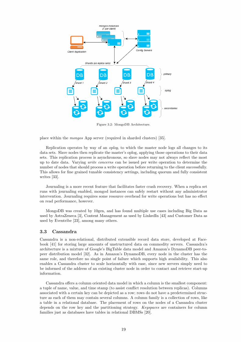
Figure 3.2: MongoDB Architecture.

place within the mongos App server (required in sharded clusters) [35].

Replication operates by way of an oplog, to which the master node logs all changes to itsdata sets. Slave nodes then replicate the master’s oplog, applying those operations to their datasets. This replication process is asynchronous, so slave nodes may not always reflect the mostup to date data. Varying write concerns can be issued per write operation to determine thenumber of nodes that should process a write operation before returning to the client successfully.This allows for fine grained tunable consistency settings, including quorum and fully consistentwrites [33].

Journaling is a more recent feature that facilitates faster crash recovery. When a replica setruns with journaling enabled, mongod instances can safely restart without any administratorintervention. Journaling requires some resource overhead for write operations but has no effecton read performance, however.

MongoDB was created by 10gen, and has found multiple use cases including Big Data asused by AstraZeneca [3], Content Management as used by LinkedIn [43] and Customer Data asused by Eventribe [23], among many others.

3.3 Cassandra

Cassandra is a non-relational, distributed extensible record data store, developed at Face-book [41] for storing large amounts of unstructured data on commodity servers. Cassandra’sarchitecture is a mixture of Google’s BigTable data model and Amazon’s DynamoDB peer-to-peer distribution model [32]. As in Amazon’s DynamoDB, every node in the cluster has thesame role, and therefore no single point of failure which supports high availability. This alsoenables a Cassandra cluster to scale horizontally with ease, since new servers simply need tobe informed of the address of an existing cluster node in order to contact and retrieve start-upinformation.

Cassandra offers a column oriented data model in which a column is the smallest component:a tuple of name, value, and time stamp (to assist conflict resolution between replicas). Columnsassociated with a certain key can be depicted as a row; rows do not have a predetermined struc-ture as each of them may contain several columns. A column family is a collection of rows, likea table in a relational database. The placement of rows on the nodes of a Cassandra clusterdepends on the row key and the partitioning strategy. Keyspaces are containers for columnfamilies just as databases have tables in relational DBMSs [20].

19

Figure 3.3: Cassandra Architecture.

Cassandra offers three main data partitioning strategies: Murmur3Partitioner, RandomPar-titioner, and ByteOrderedPartitioner [32]. The Murmur3Partitioner is the default and recom-mended strategy. It uses consistent hashing to evenly distribute data across the cluster usingan order preserving hash function. Each Cassandra node has a token value that specifies therange of keys for which they are responsible. Distributing the records evenly throughout thecluster balances the load by spreading out client requests.

Cassandra automatically replicates records throughout a cluster determined by a user spec-ified replication-factor and replication strategy. The replication strategy is important for deter-mining which nodes are responsible for which key ranges.

Client applications can contact any one node to process an operation. That node then actsas a coordinator which forwards client requests to the appropriate replica node(s) owning thedata being claimed. This mechanism is illustrated in Figure 3.3. For each write request, first acommit log entry is created. Then, the mutated columns are written to an in-memory structurecalled MemTable. A MemTable, upon reaching its size limit, is committed to disk as a newSSTable by a background process. A write request is sent to all replica nodes, however theconsistency level determines how many of them are required to respond for the transaction tobe considered complete. For a read request, the coordinator contacts a number of replica nodesspecified by the consistency level. If replicas are inconsistent the out-of-date replicas are auto-repaired in the background. In case of inconsistent replicas, a full data request is sent out andthe most recent (by comparing timestamps) version is forwarded to the client.

Cassandra is optimized for large volumes of writes as each write request is treated like anin-memory operation, while all I/O is executed as a background process. For reads, first theversions of the record are collected from all MemTables and SSTables, then consistency checksand read repair calls are performed. Keeping the consistency level low makes read operationsfaster as fewer replicas are checked before returning the call. However, read repair calls to eachreplica still happen in the background. Thus, the higher the replication factor, the more readrepair calls that are required.

Cassandra offers tunable consistency settings, which provide the flexibility for applicationdevelopers to make tradeoffs between latency and consistency. For each read and write re-quest, users choose one of the predefined consistency levels: ZERO, ONE, QUORUM, ALL orANY [41].

Cassandra implements a feature called Hinted Handoff to ensure high availability of thecluster in the event of a network partition23, hardware failure, or for some other reason. A

23A network partition is a break in the network that prevents one machine from interacting with another. Anetwork partition can be caused by failed switches, routers, or network interfaces.

20

hint contains information about a particular write request. If the coordinator node is not theintended recipient, and the intended recipient node has failed, then the coordinator node willhold on to the hint and inform the intended node when it restarts. This feature means thecluster is always available for write operations, and increases the speed at which a failed nodecan be recovered and made consistent again. [32]

Cassandra is in use at a large number of companies including Accenture [1], Coursera [17],and Spotify [67] among many others for use cases including product recommendations, frauddetection, messaging, and product catalogues.

3.4 VoltDB

VoltDB is a fully ACID compliant relational in-memory data store derived from the researchprototype H-Store [40], in use at companies like Sakura Internet [39], Shopzilla [65], and SocialGame Universe [73], among others. It has a shared nothing architecture designed to run on amulti-node cluster by dividing the data set into distinct partitions and making each node anowner of a subset of these partitions, as illustrated in Figure 3.4.

While similar to the traditional relational DBMSs of the 1970s, VoltDB is designed to takefull advantage of the modern computing environment [38]. It uses in-memory storage to max-imize throughput by avoiding costly disk-bound operations. By enforcing serialized access todata partitions (as a result of its single threaded nature), VoltDB avoids many of the time-consuming operations associated with traditional relational databases such as locking, latching,and maintaining transaction logs. Removal of these features have been highlighted by Abadi etal. [30] as key ways to significantly improve DBMS performance 24.

The unit of transactions in VoltDB is a stored procedure written and compiled as Java code,which also support a subset of ANSI-standard SQL statements. Since all data is kept in-memory,if stored procedures are directed towards the correct partition, it can execute without any I/Oor network access, providing very high throughput for transactional workloads. An additionalbenefit to stored procedures is that they ensure all transactions are fully consistent, either com-pleting or rolling-back in their entirety.

To provide durability against node failures, K-safety is a feature which duplicates data parti-tions and distributes them throughout the cluster, so that if a partition is lost (due to hardwareor software problems) the database can continue to function with the remaining duplicates.This mechanism is analogous to how other data stores replicate data based on a configuredreplication factor. Each cluster node is responsible for hosting a set number of data partitions,as determined by the sitesperhost configuration parameter. All duplicate partitions are fullyfunctioning members of the cluster however, and include all read and write privileges whichenables client applications to direct queries to any node in the cluster. Data is synchronouslycommitted to replicated partitions within the cluster before each transaction commits, thereforeensuring consistency. Duplicates function as peers similar to Cassandra’s multi-master modelrather than as slaves in a master-slave relationship used in Redis and MongoDB, and hence thereason why the architectures in Figures 3.4 (VoltDB) and 3.3 (Cassandra) look very similar.

24Abadi et al. [30] indicate that each of the following operations account for a certain percentage of the total op-erations performed by traditional relational DBMSs: Logging(11.9%), Locking(16.3%), Latching(14.2%), and BufferManagement(34.6%).

21

Figure 3.4: VoltDB Architecture.

VoltDB’s replication model is similar to K-safety, however, rather than creating redundantpartitions within a single cluster, replication creates and maintains a complete copy of the entirecluster in a separate geographic location (i.e. geo-replication). The replica cluster is intendedto take over only when the primary cluster fails completely, and as such both clusters operateindependently of each other. Replication is asynchronous and therefore does not impact theperformance of the primary cluster.

VoltDB implements a concept called command logging for transaction-level durability. Un-like write-ahead logs found in traditional systems, VoltDB logs the instantiation of commandsonly, rather than all subsequent actions. This style of logging greatly reduces the I/O load of thesystem while providing transaction-level durability either synchronously or asynchronously [37].

22

4 Experimental Setup

All experiments conducted in this study where carried out on a cluster of Virtual Machines(VM) hosted on a private cloud infrastructure within the same data center. Each Virtual Ma-chine had the same specifications and kernel settings as indicated in Table 4.1.

Setting Value

OS Ubuntu 12.04Word Length 64-bit

RAM 6 GBHard Disk 20 GB

CPU Speed 2.90GHzCores 8

Ethernet gigabitAdditional Kernel Settings atime disabled25

Table 4.1: Virtual Machine Specifications and Settings.

To assist performance analysis and cluster monitoring, a third party system monitoring toolwas installed on all VM’s to collect important system metrics while experiments were beingconducted.

Patil et al. [51] added extensions to YCSB to improve performance understanding and de-bugging of advanced NoSQL data store features by implementing a custom monitoring tool builton top of Ganglia [71]. This suggested Ganglia could be a good fit for this study also since itprovides near real time monitoring and performance metrics data for large computer networks.

Ganglia’s metric collection design mimics that of any well-designed parallel application.Each individual host in the cluster is an active participant, cooperating together, distributingthe workload while avoiding serialization and single points of failure. Ganglia’s protocol’s areoptimized at every opportunity to reduce overhead and achieve high performance [44].

Ganglia was attractive for a number of reasons including its simple implementation andconfiguration, its ability to scale easily to accommodate large cluster sizes, and its provisionof a web based user interface for fine-grained time series analysis on different metrics in aninteractive and easy way. Appendix C illustrates in more detail the precise Ganglia setup andconfiguration that was used for this study.

4.1 YCSB Configuration

In this study, one read-heavy and one write-heavy workload are included. The read-heavy work-load is one provided in the YCSB Core Package; workload B comprising a 95/5% breakdown ofread/write operations. The write-heavy workload was custom designed to consist of a 95/5%breakdown of write/read operations.

A VoltDB client driver is not currently supported by YCSB, however the VoltDB commu-nity of in-house developers built their own publicly available driver26, which was utilized in thisstudy. The VoltDB developers made several tweaks in order to effectively implement this drivercomparatively to non-relational data store systems that don’t have as strong an emphasis onserver-side logic for enhanced performance. Details of the drivers implementation is given by aVoltDB developer in [60].

The benchmarking experiments carried out by Cooper et al. in their original YCSB pa-per [14] used a fixed metric of eight threads per CPU core when running experiments. Thisnumber was considered optimal for their experiments, and after several preliminary tests wasfound to be equally optimal for this study also. If the thread count was too large, there wouldbe increased contention in the system, resulting in increased latencies and reduced throughputs.Since Redis and VoltDB have a single threaded architecture, only eight threads in total wereused by the YCSB Client, to ensure the Redis and VoltDB servers were not overwhelmed byoperation requests. This contrasts with a total of sixty-four threads which were used for bothCassandra and MongoDB experiments, which are not single threaded and can make use of all

25Disabling atime reduces the overhead of updating the last-access time of each file.26Available at https://github.com/VoltDB/voltdb/tree/master/tests/test_apps/ycsb.

23

available CPU cores27.

4.1.1 Warm-up Extension

Preliminary experiments indicated that each data store took variable lengths of time to reacha steady performance state. It was therefore deemed beneficial to implement an additionalwarm-up stage to the YCSB code base to improve results and comparative analysis. Nelubin& Engber extended YCSB to include a warm-up stage for both of their benchmarking studiesmentioned previously: [47,48]. This extended code was open sourced28 and so was subsequentlyimplemented in this study also.

In order to determine the ideal warm-up time for each data store, a set of test experimentswere repeated for each data store on various cluster sizes ranging from a single node to a twelvenode cluster. Averages of the time it took for each data store to level out at or above the overallaverage throughput of a given test experiment are summarized in Table 4.2. These warm-uptimes where subsequently passed as an additional configuration parameter to the YCSB Clientfor run phases only.

Data Store Warm-up Time (seconds)

Redis 1680MongoDB 1500Cassandra 1800

VoltDB 1200

Table 4.2: Optimal Warm-up Times For Each Data Store.

Unfortunately however, using the customized VoltDB client driver for YCSB introducedmany nontrivial incompatibility issues with the warm-up extended YCSB code base. As such,all VoltDB experiments in this study do not include a warm-up stage.

Figure 4.1 illustrates the number of operations per second that were recorded for a sampleexperiment every 10 seconds for the full duration of the experiment (10 minutes). It highlightshow long it would take for a VoltDB cluster to reach a point were it was consistently matchingor exceeding the average throughput of that experiment. This indicates a warm up period ofapproximately two minutes would be optimal and result in an increased throughput of almost1000 operations per second. The impact this had overall on VoltDB can be observed from theexperimental results presented in Section 5.4, along with comparative results among all datastores in Section 5.5.

0

2000

4000

6000

8000

10000

12000

0 100 200 300 400 500 600

Time (secs)

ops/secavg ops/sec

avg ops/sec after warm-up

Figure 4.1: VoltDB Warm-up Illustration.

4.2 Data Store Configuration and Optimization

A total of fourteen Virtual Machine nodes where provisioned for this study. One node was des-ignated for the YCSB Client, and one additional node was reserved for MongoDB configurationand App servers which are required in sharded architectures to run on separate servers to therest of the cluster. The remaining twelve nodes operated as standard cluster nodes which had

27The total number of CPU cores available on each server was 8. Using 8 threads each gives a grand total of 64threads.

28Available at https://github.com/thumbtack-technology/ycsb.

24

all four data stores installed but only one running at any given time. No other processes otherthan the Ganglia Daemon and Network Time Protocol (NTP) Daemon processes (to ensureall node clocks were synchronized) were running on cluster nodes. To ensure all nodes couldinteract effectively each node was bound to a set IP address, and known hosts of all others weremaintained on each node. To assist administrative tasks, password-less ssh was configured on allnodes also. Each data store was configured and optimized for increased throughput, low latency,and where possible to avoid costly disk-bound operations. Each subsection below discusses indetail the configurations and optimizations used for each data store.

4.2.1 Redis

Version 2.8.9 of Redis was used in this benchmark. Prior to conducting this study, Redis Clusterwas still beta quality code, and the extra processing required on the YCSB Client to interactwith the cluster was deemed too invasive on the YCSB Client and so was excluded.

To allow slave nodes to service read requests, the YCSB Client was extended to randomlypick a node (master or a slave) to send read requests to. This was determined on a per readbasis. A full code listing of this extension is illustrated in Appendix A.

Different consistency settings where enabled on each Redis node by passing the min-slaves-to-write configuration parameter to the start-up command. The value of which was determinedbased on the cluster size, and desired level of consistency. The following write consistencylevels were explored: ONE (min-slaves-to-write = 0), QUORUM (min-slaves-to-write = (clus-ter size/2)+1), and ALL (min-slaves-to-write = cluster size−1).

A complete list of configurations and optimizations that were applied for Redis experimentsare listed in Table 4.3.

Configuration Parameter Description

--appendonly no Disable AOF persistence--activerehashing no Disable active rehashing of keys. Estimated to occupy 1 ms every 100 ms

of CPU time to rehash the main Redis hash table mapping top-level keysto values

--appendfsync no Let the Operating System decide when to flush data to disk--stop-writes-on-bgsave-error no Continue accepting writes if there is an error saving data to disk--aof-rewrite-incremental-fsync no Disable incremental rewrites to the AOF filedisable snapshotting Avoiding disk-bound background jobs from interfering.

Kernel Setting Description

memory overcommitting set to 1 Recommended on the Admin section of the Redis website29

Table 4.3: Redis Configuration Settings.

4.2.2 MongoDB

Version 2.6.1 of MongoDB with the majority of all standard factory settings was used in thisstudy. Journaling however was disabled since the overhead of maintaining logs to aid crashrecovery was considered unnecessary as crash recovery was not a major consideration in thisbenchmark. If a node did crash, the experiment would simply be repeated. Additionally, thebalancer process was configured not to wait for replicas to copy and delete data during chunkmigration, in order to increase throughput when loading data onto a cluster.

MongoDB offers different write concerns for varying tunable consistency settings, of whichNORMAL, QUORUM, and ALL write concerns where explored. The YCSB Client did notsupport write concerns or read preferences, therefore the YCSB Client was extended to facili-tate them. A code listing of these extensions are given in Appendix B. For all experiments theprimary preferred read preference was used to favor queries hitting the master preferably, but iffor whatever reason the master was unavailable, requests would be routed to a replicated slave.Write concerns and read preferences where passed as additional command line parameters tothe YCSB Client.

29http://redis.io/topics/admin

25

As suggested at the beginning of this subsection, additional configuration and App serversare required for sharded MongoDB clusters. The recommended production setup is to havethree configuration servers all located on separate hosts, and at least one App server per client.For the purpose of this benchmark study, only one configuration server was used and resided onthe same host as a single App server which the YCSB Client interacted with exclusively. Thissetup seemed appropriate for this study since having only one configuration server is adequatefor development environments [34], and it was observed that having both reside on the samehost did not prove to be a bottleneck.

The shard key used was the default index key (‘ id ’) enforced by MongoDB and subsequentlythe key used by YCSB to insert, read and update records.

4.2.3 Cassandra

For this benchmark, version 1.2.16 (the latest 1.X release available before commencing thisstudy) of Cassandra was used because the latest version supported by the YCSB Cassandraclient driver was 1.X; even though the current release of Cassandra has progressed to version2.0.9. This unfortunately meant that the performance enhancements available in verion 2.0could not be assesed30. Nonetheless, most of the default configurations where used except thosementioned below.

A token representing the range of data each node would be responsible for in each inde-pendent cluster configuration was pre-calculated and saved in separate copies of a Cassandraconfiguration file. The configuration file specific to the cluster setup required for a given ex-periment was then passed to Cassandra at start-up time. This was necessary to overcome theproblems associated with Cassandra attempting to define these distinct partitions itself as newnodes were added to a cluster, which become evident during preliminary testing. These tokenswere calculated using a token generator tool31, using the Murmur3 partitioner (which distributesdata across a cluster evenly using the Murmur3 128 hash function32) and passing as a parameterthe number of nodes in the cluster.

Hinted-handoff was disabled on all nodes within the cluster to avoid the situation were a nodecould fail and remain offline for the duration of an experiment, causing hints to build up rapidlyas the YCSB Client attempted to saturate the cluster. Preliminary testing indicated that sucha situation often led to detrimental impact and increased instability throughout the cluster. Inkeeping with the rule of rerunning experiments that are subjected to failures; it seemed rea-sonable to disable hinted-handoffs and therefore avoid the additional overhead associated with it.

Additional configuration optimizations included increasing the maximum number of con-current reads and writes to match the same number of threads used by YCSB Client i.e. 64.Finally, the RPC server type was changed to ‘hsha’ to reduce to amount of memory used byeach Cassandra node; ideal for scaling to large clusters.

Three Java JVM setting changes included: setting the JVM heap size to 4GB (to approxi-mately match the amount of memory used by each node); setting the heap new size to 800MB(100MB per core); and finally disabling all assertions in order to increase performance.

4.2.4 VoltDB

In this study version 4.4 of the VoltDB Enterprise edition was used with its default configura-tions, including asynchronous command logging. For illustrative purposes, the VoltDB plots ofSection 5.4 include comparative results for experiments conducted without command loggingor replication. A constant number of distinct data partitions per host was used based on therecommendation of approximately 75% of the number of available cores on each server [38].

30For a complete description of the internal optimizations and improvements featured in Cassandra 2.0, see:http://www.datastax.com/dev/blog/whats-under-the-hood-in-cassandra-2-0, Last Accessed: 2014.08.27

31http://www.geroba.com/cassandra/cassandra-token-calculator/32An informative description can be found here: http://code.google.com/p/smhasher/wiki/MurmurHash3, Last

Accessed: 19/08/2014

26

This amounted to approximately six partitions per host.

VoltDB’s implementation of replication is primarily for geo-replication if an entire data cen-ter cluster falls over. VoltDB’s method of inter-data center partition replication is referred to asK-Safety and is analogous to how other data stores handle partition replication. Therefore, K-Safety was the feature used to evaluate the performance impact of replication within a VoltDBcluster in this study. Since VoltDB is fully ACID compliant, partition replicas remain consis-tent by nature regardless of the replication factor. Consequently, VoltDB does not offer tunableconsistency settings and therefore, different consistency levels could not be explored further.

4.3 Methodology

The experiments carried out in this study include the three different data distributions men-tioned in Section 2, each simulating a different industry application use case. Two differentworkloads (one read-heavy and one write-heavy) were used, and each cluster node hosted enoughdata to utilize a minimum of 80% RAM. Disk-bound operations were not considered since Redisand VoltDB are designed to have all data kept in memory.

MongoDB was configured to have a constant replication factor of two replicas per shard,meeting the minimum recommended production settings. The number of shards were incre-mented from 1 to 4, in order to directly explore the write-scalability of MongoDB.

An equivalent setup could have been established for Redis using the soon to be releasedRedis Cluster (still currently in beta testing). After experimenting with the beta version ofRedis Cluster, it became apparent that reads rely too heavily on client side processing. In theinterest of not laboring the YCSB Client with this task and subsequently skewing results, itwas decided that Redis Cluster would not be explored further. Subsequently, a basic set ofreplication experiments were conducted which for a given cluster size, consisted of assigning onenode to be the master and having the remaining nodes all act as replicas.

Cassandra and VoltDB offer greater flexibility in replicating data partitions due to theirmulti-master architectures and ability to have multiple partitions held on a single node. Assuch, less trivial experiments could be performed. Details of which are indicated in Table 4.4.

The precise set of experiments conducted for all data stores in this study are summarizedin Table 4.4. Each permutation of the experiments listed were repeated a minimum of threetimes. Additional repeats of experiments, up to a maximum of ten, were scheduled if the resultsfrom three repeats showed considerable anomalies (for example due to instability of the cloudenvironment or because of node failure).

Redis MongoDB Cassandra VoltDBWorkload

Read Heavy (G)Write Heavy (H)

ConsistencyONE

QUORUMALL

DistributionUniform

ZipfianLatest

Cluster Size 1 3 6 9 12 1 3 6 9 12 1 3 6 9 12 1 3 6 9 12Replication Factor 0 2 5 8 11 0 2 2 2 2 0 2 4 6 8 0 2 4 6 8Number Of Partitions33 1 1 2 3 4 6 18 36 54 72Distinct Partitions 1 1 2 3 4 6 9 9 9 9Base Line Experiment

Table 4.4: Complete List of Experiments.

Additional base line experiments were carried out in order to have a basis for comparison,a key determinant in evaluating the performance impact of replication per Cooper et al. [14].

33Applicable to MongoDB and VoltDB only. In MongoDB, a partition is another name for a shard. In VoltDBeach node is partitioned into a number of ‘sites per host’ which applies to each node in the cluster. Therefore the totalnumber of partitions shown is across the whole cluster, each node being responsible for 6 individual partitions/sites.

27

These base line experiments consisted of maintaining the same cluster sizes, with no replication,using the uniform distribution only, for all applicable consistency levels. Redis, unfortunatelydoes not support multiple partitions and as such, additional base line experiments could not beincluded.

Prior to conducting experiments, a number of load tests were carried out to identify theamount of data required to utilize 80% RAM on all nodes within a given cluster for each datastore, and the optimal number of threads the YCSB Client should use when loading this dataonto the cluster.

The following steps outline the procedure that was carried out for each experiment. A num-ber of bash scripts where written to automate these steps and all experiments highlighted inTable 4.4 for each data store. Once all experiments had been conducted three times, the resultswould be analyzed, anomalies identified and new automated scripts generated to rerun thoseexperiments following the same steps highlighted below:

1. Start up a fresh cluster of the correct size and replication factor specific to the experimentin question.

2. Delay for a short period of time to ensure all nodes within the cluster have been fullyconfigured and are ready to accept requests.

3. Load the data store cluster with sample data based on the factors indicated by load testsconducted previously.

4. Run the given experiment workload for a preconfigured warm-up time in order for thecluster to reach optimal throughput before starting the official test.

5. Run the experiment specifying a maximum execution time of 10 minutes.

6. Allow a short cool down period to ensure all actions related to the experiment have beencompleted.

7. Collect and backup results of the experiment conducted in step 5.

8. Tear down the entire cluster and wipe all data associated with the experiment on eachnode.

9. Repeat steps 1 to 8 until all experiments have been carried out a minimum number oftimes.

28

5 Experimental Results

YCSB reports the results of an experiment by printing them to the standard output terminalevery 10 seconds. These were subsequently redirected to log files and an additional set of scriptswere written to parse the output into a more amenable format for analysis. Where possible, thenumber of experiment reruns were kept below 7 additional runs. However due to varying levelsof stability of each data store on the private cloud environment utilized in this study a numberof rerun’s were inevitable.

Redis was the most stable data store, which becomes clear when we consider the 95th%confidence interval figures presented in Table 5.2 later in this section. Cassandra was alsovery stable with minimal experiment failures and minimal supervision while experiments wererunning. However a number of repeated experiments were required, again obvious from the95th% confidence interval figures presented in Table 5.8 later in this section.

MongoDB and VoltDB required considerable levels of supervision and intervention whileexperiments where conducted. For VoltDB specifically, if a sinlge or multi node crash wasexperienced, the YCSB Client was unable to continue conducting the experiment correctly eventhough VoltDB clusters are able to function when a node fails. Similarly, MongoDB failuresoften increased the instability of an experiment and required manual intervention to preventthe YCSB Client from hanging indefinitely and subsequently saturating disk space by spewingerrors into the MongoDB logs.

In this section, the results of each data store will be discussed and analyzed in-depth followedby a presentation of several key features that are comparative among all four data stores.

5.1 Redis

Since baseline experiments could not be conducted for Redis, we are unable to evaluate the im-pact replication has on performance relative to non-replicated clusters of equal size. Nonetheless,some interesting observations have been made regarding the impact on availability that repli-cation has for read and write operations.

Adding 2 additional nodes as replicas to a single node cluster resulted in an increase inperformance on the read-heavy workload (G). On a single node cluster, the average throughputacross all distributions and consistency levels is 23708.33 ops/sec which increases by 45.2% onaverage when an additional 2 nodes are added as slaves. This is expected since these additionalnodes are able to service read requests i.e. reads have been scaled horizontally. However, asadditional slaves are added to a cluster beyond size 3, the read performance remains fairlyconstant. On average, throughputs are equal to 28846.3, 43136.2, and 42605 ops/sec for ONE,QUORUM, and ALL consistency levels respectively for all cluster sizes with a replication factorgreater than 0. These relate to minimal standard deviations of 440.1 (1.53%), 678.2 (1.57%),and 966.8 (2.27%) ops/sec respectively. Due to Redis’ master-slave replication model, the YCSBClient is only able to pick one node at random to send a read request to. Therefore performanceis unable to benefit from a further increase in the number of slaves. If more clients were inter-acting with the cluster, we would potentially observe an increase in throughput. This suggeststhat read operations remain highly and consistently available as the replication factor increases.

We observe in the read-heavy workload (G) that QUORUM and ALL consistency levels havefairly equal performances. Throughputs across all cluster sizes and distributions average 39034.7ops/sec with a standard deviation of only 297.4 (0.76%) ops/sec. Read and write latenciesaverage at 0.2107 ms and 0.2050 ms with standard deviations of 0.00108 (0.5%) ms and 0.00141(0.7%) ms respectively. Different consistency settings are not expected to have an impact onread operations, due to a lack of support in Redis, therefore we expect the throughputs to besimilar.

A noticeable contradiction is apparent when we consider the trends exhibited by workloadG in Figure 5.1. That it, consistency level ONE is on average 39.1% less performant than QUO-RUM and ALL consistency levels on cluster sizes greater than 1. There is also an increase inread and write latencies c.f. Figures 5.2 and 5.3. The only difference between these experimentsis that the min-slaves-to-write configuration setting is disabled for consistency level ONE. Thisappears to be an anomaly of some sort since there is nothing in the Redis source code thatsuggests a decline in performance would result from disabling this option. However, the Redis

29

15000

20000

25000

30000

35000

40000

45000

1 3 6 9 12

Th

rou

ghp

ut

(op

s/se

c)

Cluster Size

workloadg uniformworkloadg zipfianworkloadg latest

workloadh uniformworkloadh zipfianworkloadh latest

(a)

15000

20000

25000

30000

35000

40000

45000

1 3 6 9 12

Th

rou

ghp

ut

(op

s/se

c)

Cluster Size



(b)

15000

20000

25000

30000

35000

40000

45000

1 3 6 9 12

Th

rou

gh

pu

t(o

ps/

sec)

Cluster Size



(c)

Figure 5.1: Redis: Overall Throughputs per Consistency Level for all Workloads and Distributions: (a) ONE (b) QUORUM(c) ALL.

200

250

300

350

400

450

500

1 3 6 9 12

Late

ncy

(ms)

Cluster Size



(a)

200

250

300

350

400

450

500

1 3 6 9 12

Lat

ency

(ms)

Cluster Size



(b)

200

250

300

350

400

450

500

1 3 6 9 12

Lat

ency

(ms)

Cluster Size



(c)

Figure 5.2: Redis: Read Latencies per Consistency Level for all Workloads and Distributions: (a) ONE (b) QUORUM (c) ALL.

release notes34 indicate that a major issue had been discovered relating to the min-slaves-to-writeoption, present in the Redis version used in this study. A fresh set of results where gatheredusing the most recent Redis version (2.8.13) which had this issue resolved, however the resultsshowed identical trends.

Overall throughput on the write-heavy workload (H) degrades as the cluster size increases.Considering the figures presented in Table 5.2, there is a 19.2% decrease in throughput on av-erage each time the cluster size increases by 3 nodes, independent of the consistency level ordistribution. This is likely a result of more slaves interacting with the master and the mech-anism in which slaves process new data. When each slave receives new data from the master(asynchronously in the background), once it is ready to replace its stale version of the data, theslave blocks waiting on the replacement to take place. As such read throughput will decreaseand subsequent writes will be delayed due to the single threaded architecture of Redis. Theresults suggest that the availability for write operations will continue to be affected as additionalslaves are added to the cluster.

For the write-heavy workload (H) consistency levels ONE, QUORUM, and ALL are allpretty similar. They each have throughputs averaging 25882.7 ops/sec across all cluster sizesand distributions, with a standard deviation of only 54.1 (0.2%) ops/sec between them. Thisis because Redis only offers a relaxed form of consistency for writes only, with no guarantees.When processing a write operation the master simply checks an internal hash table to ensure aset number of slaves, determined by the consistency level, pinged the master within the previous10 second interval. This would be a pretty constant time operation regardless of the cluster sizeand consistency requirements.

We observe minimal differences in overall throughput between distributions for both work-loads. Observing an average difference of only 1.7%, and 1.3% between distributions across allcluster sizes and consistency levels for workload G and H respectively and standard deviationsof 1.2% and 1% respectively for workload G and H. Table 5.1 gives the details of this compar-

34Available here: http://download.redis.io/redis-stable/00-RELEASENOTES. Last accessed: 12/08/2014

30

200

250

300

350

400

450

500

1 3 6 9 12

Lat

ency

(ms)

Cluster Size



(a)

200

250

300

350

400

450

500

1 3 6 9 12

Lat

ency

(ms)

Cluster Size



(b)

200

250

300

350

400

450

500

1 3 6 9 12

Late

ncy

(ms)

Cluster Size



(c)

Figure 5.3: Redis: Write Latencies per Consistency Level for all Workloads and Distributions: (a) ONE (b) QUORUM (c)ALL.

ison. The likely reason for this is because Redis keeps all data in memory on a single server.Subsequently, requests to access or update records of varying distributions will result in thesame action: performing a constant time operation on a single hash table. As with all hashtables, this constant time operation is characterized by an asymptotic run time of O(1) in theaverage case.

As illustrated in Figure 5.1 and supported by the data in Table 5.3, on a single node clusterthe write-heavy workload (H) outperforms the read-heavy workload (G) by 43.7% on averageacross all distributions and consistency levels, with a standard deviation of only 0.3%. Thisis as a direct result of how the YCSB Client interacts differently with a Redis cluster for readand write operations. Read operations will access all the fields a particular key maps (to 10in this case), as opposed to write operations which only update 1 field. This suggests that forone node, there is a 4.85% decline in performance for each additional field that needs read sinceRedis must traverse the key list searching for a repeated key and its required associated field.

However, when replicas are added to a cluster, the read-heavy workload (G) starts to out-perform the write-heavy workload (H), averaging 48.9% increases across all subsequent clustersizes for all distributions and consistency levels. This correlates to a 24.4%, 61.8%, and 60.5%increase for ONE, QUORUM, and ALL consistency levels respectively, and 49.3%, 49.1%, and48.2% increases for the uniform, zipfian, and latest distributions respectively. This increase inperformance is due to the ability of additional slaves to service read requests. Whereas only onesingle-threaded master can process write requests which in workload H acts as a bottleneck dueto the large percentage of write operations (95%).

The availability of write operations does not appear to be affected by the percentage of readoperations in a given workload and vice versa. We observe a 37.1% (0.115 ms) decrease in writelatencies for Workload G (5% writes) compared to Workload H (95% writes), and a 40.8% (0.108ms) reduction in read latencies in workload H (5% reads) compared to workload G (95% reads).This is not a proportional decrease since the overhead of the underlying operation remains thesame i.e. a hash table lookup. The additional overhead is a direct result of the single threadednature of Redis which is forced to contend with an increase in the number of operations it mustservice. Writes are more affected since all writes must be directed to a single master instance.

Figures 5.4, 5.5, 5.6, and 5.7 illustrate the latency histograms for read and write operationson both workloads. As we can see from the CDF curves plotted on the same figures, 95% ofoperations can be answered in less than 1 ms for all cluster sizes, distributions, and workloads.The 95th percentile figures are subsequently not included in Table 5.2 for the sake of brevity.

31

Workload G Workload H

Cluster Size 1 3 6 9 12 1 3 6 9 12

Replication Factor 0 2 5 8 11 0 2 5 8 11

Type Metric Distribution Consistency

Read Latency Uniform vs Zipfian ONE 0.3 2.1 0.0 0.4 1.1 0.9 1.7 9.2 16.7 12.9Uniform vs Latest 1.2 2.1 1.1 1.8 1.9 2.7 4.4 4.0 8.9 8.4Uniform vs Zipfian ALL 0.3 1.1 3.3 2.2 4.5 1.3 4.4 1.6 6.4 9.1Uniform vs Latest 1.5 3.7 3.3 2.8 2.3 2.7 3.3 8.5 4.7 7.8Uniform vs Zipfian QUORUM 1.2 0.0 1.1 0.6 2.8 1.3 1.0 3.1 4.1 4.8Uniform vs Latest 2.1 4.4 0.6 1.7 3.4 2.2 0.0 3.6 11.4 8.3

Write Latency Uniform vs Zipfian ONE 0.0 2.3 1.0 0.0 0.7 0.0 0.4 0.9 0.8 1.0Uniform vs Latest 0.9 3.3 1.0 2.0 1.3 0.9 2.7 1.8 1.3 2.1Uniform vs Zipfian ALL 0.3 1.8 0.4 4.4 0.0 0.5 0.8 0.6 0.0 1.9Uniform vs Latest 1.2 3.6 1.8 1.7 3.3 0.9 2.3 0.6 0.8 0.8Uniform vs Zipfian QUORUM 1.5 0.5 4.2 4.3 0.8 0.5 0.8 2.1 2.0 0.4Uniform vs Latest 2.1 7.0 0.0 3.4 3.7 1.4 0.4 0.9 3.5 4.4

Overall Throughput Uniform vs Zipfian ONE 0.2 1.8 0.1 0.5 0.7 0.3 0.2 0.7 1.2 1.1Uniform vs Latest 1.2 1.8 0.9 1.9 1.5 1.3 2.5 1.9 1.5 2.2Uniform vs Zipfian ALL 0.4 0.7 3.2 2.1 4.3 0.4 1.0 0.6 0.1 2.2Uniform vs Latest 1.4 3.5 3.2 2.3 1.8 1.0 1.9 0.4 0.9 0.6Uniform vs Zipfian QUORUM 1.1 0.1 2.0 0.7 2.3 0.1 0.5 2.6 1.9 0.5Uniform vs Latest 2.1 4.3 0.7 1.6 3.0 1.1 0.2 1.2 3.1 4.4

Table 5.1: Redis: Percentage Differences In Read & Write Latencies and Overall Throughput Between Distributions for eachWorkload and Consistency Level.


Cluster Size 1 3 6 9 12 1 3 6 9 12



Read Latency (ms) Uniform ONE 0.335 0.283 0.273 0.275 0.271 0.228 0.23 0.227 0.234 0.223QUORUM 0.338 0.179 0.177 0.18 0.181 0.228 0.203 0.189 0.199 0.214ALL 0.336 0.184 0.177 0.184 0.172 0.229 0.211 0.192 0.194 0.199

Zipfian ONE 0.334 0.277 0.273 0.274 0.268 0.226 0.234 0.207 0.198 0.196QUORUM 0.334 0.179 0.179 0.179 0.176 0.225 0.201 0.195 0.191 0.204ALL 0.335 0.182 0.183 0.18 0.18 0.226 0.202 0.189 0.182 0.218

Latest ONE 0.331 0.277 0.27 0.27 0.266 0.222 0.22 0.218 0.214 0.205QUORUM 0.331 0.187 0.178 0.177 0.175 0.223 0.203 0.196 0.223 0.197ALL 0.331 0.191 0.183 0.179 0.176 0.223 0.218 0.209 0.185 0.184

Write Latency (ms) Uniform ONE 0.341 0.307 0.292 0.303 0.303 0.212 0.263 0.332 0.399 0.484QUORUM 0.344 0.208 0.212 0.236 0.247 0.213 0.26 0.329 0.406 0.486ALL 0.342 0.22 0.223 0.232 0.25 0.213 0.261 0.336 0.393 0.475



Overall Throughput Uniform ONE 23633 27922 28919 28610 29065 36829 30221 24262 20282 16869QUORUM 23429 43245 43853 42733 42607 36816 30717 24655 20043 16813ALL 23558 42079 43501 41961 44416 36670 30494 24036 20682 17220

Zipfian ONE 23684 28443 28902 28741 29260 36933 30296 24081 20523 17062QUORUM 23679 43286 42992 43053 43594 36867 30878 24034 20433 16905ALL 23655 42383 42144 42852 42553 36825 30786 24172 20705 16840

Latest ONE 23910 28441 29186 29152 29514 37309 30999 23814 20579 17245QUORUM 23933 41404 43536 43430 43901 37226 30767 24351 20672 17564ALL 23894 40649 42150 42953 43619 37047 31086 24124 20871 17117

95% CI Uniform ONE 0 3.92 0 1.96 1.96 1.96 3.92 3.92 0 0QUORUM 0 1.96 0 1.96 1.96 1.96 3.92 9.8 0 1.96ALL 0 5.88 5.88 1.96 0 3.92 5.88 0 0 0

Zipfian ONE 0 1.96 0 1.96 1.96 0 5.88 0 1.96 0QUORUM 0 0 5.88 0 1.96 1.96 3.92 1.96 1.96 1.96ALL 0 7.84 3.92 0 5.88 1.96 5.88 0 0 0

Latest ONE 0 1.96 0 0 0 1.96 3.92 0 0 0QUORUM 0 5.88 5.88 1.96 0 1.96 5.88 3.92 1.96 0ALL 0 13.72 1.96 5.88 0 0 3.92 0 0 3.92

Table 5.2: Redis: Read & Write Latency and Overall Throughput & 95th% Confidence Interval Data per Workload, BrokenDown by Distribution and Consistency Level.

32

Cluster Size 1 3 6 9 12

Replication Factor 0 2 5 8 11


Read Latency Uniform ONE 38.0 20.7 18.4 16.1 19.4QUORUM 38.9 12.6 6.6 10.0 16.7ALL 37.9 13.7 8.1 5.3 14.6

Zipfian ONE 38.6 16.8 27.5 32.2 31.0QUORUM 39.0 11.6 8.6 6.5 14.7ALL 38.9 10.4 3.2 1.1 19.1

Latest ONE 39.4 22.9 21.3 23.1 25.9QUORUM 39.0 8.2 9.6 23.0 11.8ALL 39.0 13.2 13.3 3.3 4.4

Write Latency Uniform ONE 46.7 15.4 12.8 27.4 46.0QUORUM 47.0 22.2 43.3 53.0 65.2ALL 46.5 17.0 40.4 51.5 62.1



Overall Throughput Uniform ONE 43.7 7.9 17.5 34.1 53.1QUORUM 44.4 33.9 56.0 72.3 86.8ALL 43.5 31.9 57.6 67.9 88.2



Table 5.3: Redis: Percentage Differences In Read & Write Latencies and Overall Throughput Between Workloads for eachDistribution and Consistency Level.

1

10

100

1000

10000

100000

1e+06

1e+07

1e+08

1 10 100 10000

20

40

60

80

100

Num

ber

Of

Op

erat

ions

CD

F(%

)

Latency (ms)

1 node3 nodes6 nodes9 nodes

12 nodes

(a)

1

10

100

1000

10000

100000

1e+06

1e+07

1e+08

1 10 100 10000

20

40

60

80

100

Num

ber

Of

Op

erat

ions

CD

F(%

)

Latency (ms)


12 nodes

(b)

1

10

100

1000

10000

100000

1e+06

1e+07

1e+08

1 10 100 10000

20

40

60

80

100N

um

ber

Of

Op

erat

ions

CD

F(%

)

Latency (ms)


12 nodes

(c)

1

10

100

1000

10000

100000

1e+06

1e+07

1e+08

1 10 100 10000

20

40

60

80

100

Num

ber

Of

Op

erat

ions

CD

F(%

)

Latency (ms)


12 nodes

(d)

1

10

100

1000

10000

100000

1e+06

1e+07

1e+08

1 10 100 10000

20

40

60

80

100

Num

ber

Of

Op

erat

ions

CD

F(%

)

Latency (ms)


12 nodes

(e)

1

10

100

1000

10000

100000

1e+06

1e+07

1e+08

1 10 100 10000

20

40

60

80

100

Num

ber

Of

Op

erat

ions

CD

F(%

)

Latency (ms)


12 nodes

(f)

1

10

100

1000

10000

100000

1e+06

1e+07

1e+08

1 10 100 10000

20

40

60

80

100

Num

ber

Of

Op

erat

ions

CD

F(%

)

Latency (ms)


12 nodes

(g)

1

10

100

1000

10000

100000

1e+06

1e+07

1e+08

1 10 100 10000

20

40

60

80

100

Num

ber

Of

Op

erat

ions

CD

F(%

)

Latency (ms)


12 nodes

(h)

1

10

100

1000

10000

100000

1e+06

1e+07

1e+08

1 10 100 10000

20

40

60

80

100

Num

ber

Of

Op

erat

ions

CD

F(%

)

Latency (ms)


12 nodes

(i)

Figure 5.4: Redis Workload G Read Latency Histograms: (a) Uniform ONE (b) Uniform QUORUM (c) Uniform ALL (d)Zipfian ONE (e) Zipfian QUORUM (f) Zipfian ALL (g) Latest ONE (h) Latest QUORUM (i) Latest ALL.

33

1

10

100

1000

10000

100000

1e+06

1e+07

1e+08

1 10 100 10000

20

40

60

80

100N

um

ber

Of

Op

erati

ons

CD

F(%

)

Latency (ms)


12 nodes

(a)

1

10

100

1000

10000

100000

1e+06

1e+07

1e+08

1 10 100 10000

20

40

60

80

100

Num

ber

Of

Op

erati

ons

CD

F(%

)

Latency (ms)


12 nodes

(b)

1

10

100

1000

10000

100000

1e+06

1e+07

1e+08

1 10 100 10000

20

40

60

80

100

Num

ber

Of

Op

erati

ons

CD

F(%

)

Latency (ms)


12 nodes

(c)

1

10

100

1000

10000

100000

1e+06

1e+07

1e+08

1 10 100 10000

20

40

60

80

100

Num

ber

Of

Op

erat

ions

CD

F(%

)

Latency (ms)


12 nodes

(d)

1

10

100

1000

10000

100000

1e+06

1e+07

1e+08

1 10 100 10000

20

40

60

80

100

Num

ber

Of

Op

erat

ions

CD

F(%

)

Latency (ms)


12 nodes

(e)

1

10

100

1000

10000

100000

1e+06

1e+07

1e+08

1 10 100 10000

20

40

60

80

100

Num

ber

Of

Op

erat

ions

CD

F(%

)

Latency (ms)


12 nodes

(f)

1

10

100

1000

10000

100000

1e+06

1e+07

1e+08

1 10 100 10000

20

40

60

80

100

Num

ber

Of

Op

erat

ions

CD

F(%

)

Latency (ms)


12 nodes

(g)

1

10

100

1000

10000

100000

1e+06

1e+07

1e+08

1 10 100 10000

20

40

60

80

100

Num

ber

Of

Op

erat

ions

CD

F(%

)Latency (ms)


12 nodes

(h)

1

10

100

1000

10000

100000

1e+06

1e+07

1e+08

1 10 100 10000

20

40

60

80

100

Num

ber

Of

Op

erat

ions

CD

F(%

)

Latency (ms)


12 nodes

(i)

Figure 5.5: Redis Workload G Write Latency Histograms: (a) Uniform ONE (b) Uniform QUORUM (c) Uniform ALL (d)Zipfian ONE (e) Zipfian QUORUM (f) Zipfian ALL (g) Latest ONE (h) Latest QUORUM (i) Latest ALL.

1

10

100

1000

10000

100000

1e+06

1e+07

1e+08

1 10 100 10000

20

40

60

80

100

Num

ber

Of

Op

erat

ions

CD

F(%

)

Latency (ms)


12 nodes

(a)

1

10

100

1000

10000

100000

1e+06

1e+07

1e+08

1 10 100 10000

20

40

60

80

100

Num

ber

Of

Op

erat

ions

CD

F(%

)

Latency (ms)


12 nodes

(b)

1

10

100

1000

10000

100000

1e+06

1e+07

1e+08

1 10 100 10000

20

40

60

80

100

Num

ber

Of

Op

erat

ions

CD

F(%

)

Latency (ms)


12 nodes

(c)

1

10

100

1000

10000

100000

1e+06

1e+07

1e+08

1 10 100 10000

20

40

60

80

100

Num

ber

Of

Op

erat

ions

CD

F(%

)

Latency (ms)


12 nodes

(d)

1

10

100

1000

10000

100000

1e+06

1e+07

1e+08

1 10 100 10000

20

40

60

80

100

Num

ber

Of

Op

erat

ions

CD

F(%

)

Latency (ms)


12 nodes

(e)

1

10

100

1000

10000

100000

1e+06

1e+07

1e+08

1 10 100 10000

20

40

60

80

100

Num

ber

Of

Op

erat

ions

CD

F(%

)

Latency (ms)


12 nodes

(f)

1

10

100

1000

10000

100000

1e+06

1e+07

1e+08

1 10 100 10000

20

40

60

80

100

Num

ber

Of

Op

erat

ions

CD

F(%

)

Latency (ms)


12 nodes

(g)

1

10

100

1000

10000

100000

1e+06

1e+07

1e+08

1 10 100 10000

20

40

60

80

100

Num

ber

Of

Op

erat

ions

CD

F(%

)

Latency (ms)


12 nodes

(h)

1

10

100

1000

10000

100000

1e+06

1e+07

1e+08

1 10 100 10000

20

40

60

80

100

Num

ber

Of

Op

erat

ions

CD

F(%

)

Latency (ms)


12 nodes

(i)

Figure 5.6: Redis Workload H Read Latency Histograms: (a) Uniform ONE (b) Uniform QUORUM (c) Uniform ALL (d)Zipfian ONE (e) Zipfian QUORUM (f) Zipfian ALL (g) Latest ONE (h) Latest QUORUM (i) Latest ALL.

34

1

10

100

1000

10000

100000

1e+06

1e+07

1e+08

1 10 100 10000

20

40

60

80

100

Num

ber

Of

Op

erati

ons

CD

F(%

)

Latency (ms)


12 nodes

(a)

1

10

100

1000

10000

100000

1e+06

1e+07

1e+08

1 10 100 10000

20

40

60

80

100

Num

ber

Of

Op

erati

ons

CD

F(%

)

Latency (ms)


12 nodes

(b)

1

10

100

1000

10000

100000

1e+06

1e+07

1e+08

1 10 100 10000

20

40

60

80

100

Num

ber

Of

Op

erati

ons

CD

F(%

)

Latency (ms)


12 nodes

(c)

1

10

100

1000

10000

100000

1e+06

1e+07

1e+08

1 10 100 10000

20

40

60

80

100

Num

ber

Of

Op

erat

ions

CD

F(%

)

Latency (ms)


12 nodes

(d)

1

10

100

1000

10000

100000

1e+06

1e+07

1e+08

1 10 100 10000

20

40

60

80

100

Num

ber

Of

Op

erat

ions

CD

F(%

)

Latency (ms)


12 nodes

(e)

1

10

100

1000

10000

100000

1e+06

1e+07

1e+08

1 10 100 10000

20

40

60

80

100

Num

ber

Of

Op

erat

ions

CD

F(%

)

Latency (ms)


12 nodes

(f)

1

10

100

1000

10000

100000

1e+06

1e+07

1e+08

1 10 100 10000

20

40

60

80

100

Num

ber

Of

Op

erat

ions

CD

F(%

)

Latency (ms)


12 nodes

(g)

1

10

100

1000

10000

100000

1e+06

1e+07

1e+08

1 10 100 10000

20

40

60

80

100

Num

ber

Of

Op

erat

ions

CD

F(%

)

Latency (ms)


12 nodes

(h)

1

10

100

1000

10000

100000

1e+06

1e+07

1e+08

1 10 100 10000

20

40

60

80

100

Num

ber

Of

Op

erat

ions

CD

F(%

)

Latency (ms)


12 nodes

(i)

Figure 5.7: Redis Workload H Write Latency Histograms: (a) Uniform ONE (b) Uniform QUORUM (c) Uniform ALL (d)Zipfian ONE (e) Zipfian QUORUM (f) Zipfian ALL (g) Latest ONE (h) Latest QUORUM (i) Latest ALL.

35













Table 5.4: MongoDB: Percentage Differences In Read & Write Latencies and Overall Throughput Between Workloads for eachDistribution and Consistency Level.

5.2 MongoDB

The read-heavy workload (G) has on average an 88.7% higher level of throughput than the write-heavy workload (H). This corresponds to 94.8%, 84%, and 87.2% increases for uniform, zipfian,and latest distributions respectively, on average across all consistency levels and cluster sizes.When broken down by consistency level, we can observe a 89.5%, 87.1%, and 89.5% increase forONE, QUORUM, and ALL consistency levels respectively. Figure 5.8 illustrates how this trendvaries as the cluster size increases, while Table 5.4 gives more in-depth information per clustersize.

These trends are due to MongoDB’s contrasting concurrency mechanism for reads and writes.MongoDB allows for concurrent reads on a collection, but enforces a single threaded lockingmechanism on all write operations to ensure atomicity. In addition, all write operations needto be appended to an oplog on disk, which involves a greater overhead. The oplog is critical forreplicas to maintain an accurate and complete copy of the primary shard’s data. Furthermore,regardless of the requested read concern no additional consistency checks are performed betweenreplicas on read operations.

For both workloads we observe a performance drop from cluster sizes 1 to 3. This is due toan additional replication factor of 2 being applied to a single shard (i.e. in the 3 node cluster).The original shard in the single node cluster now needs to save data to an oplog on disk andmanage 2 additional servers. However, for cluster sizes greater than 3 nodes, more shards areable to distribute the load of reads and writes.

We subsequently see an increase in performance in line with non-replicated clusters of equalsize when the cluster size is greater than 3. On average a 3 node cluster has a 91.8% and 87.7%decrease in throughput across all distributions and consistency levels for workload G and Hrespectively compared to non-replicated clusters of equal size. Meanwhile, on all subsequentcluster sizes (6+), the average decrease in throughput is only 13.6% and 40.3% for workloadG and H respectively. This suggests that replication has a minimal affect on performance inread-heavy workloads once the overhead of maintaining a small number of shards have beenovercome. This impact is more noticeable for write-heavy workloads however since consistencychecks are performed on writes. Table 5.6 illustrates these observations at a more granular level.

Read and write latencies for the read-heavy (G) and write-heavy (H) workloads follow simi-lar trends, as illustrated in Figures 5.9 and 5.10. However, on average workload H has 8.7% and56.7% increases in read and write latencies respectively across all cluster sizes, distributions and

36

0

5000

10000

15000

20000

25000

30000

35000

1 3 6 9 12

Th

rou

gh

pu

t(o

ps/

sec)

Cluster Size


workloadh uniform

workloadh zipfianworkloadh latest

workloadg no-replworkloadh no-repl

(a)

0

5000

10000

15000

20000

25000

30000

35000

1 3 6 9 12

Th

rou

gh

pu

t(o

ps/

sec)

Cluster Size


workloadh uniform



(b)

0

5000

10000

15000

20000

25000

30000

35000

1 3 6 9 12

Th

rou

ghp

ut

(op

s/se

c)

Cluster Size


workloadh uniform



(c)

Figure 5.8: MongoDB: Overall Throughputs per Consistency Level for all Workloads and Distributions: (a) ONE (b) QUORUM(c) ALL.

consistency levels compared to workload G. On an individual distribution level, read latenciesare increased by 18%, 3.8%, and 2.1% for uniform, zipfian, and latest distributions respectivelyacross all cluster sizes. Similarly, write latencies have a 63.9%, 51.2%, and 53.6% increases foruniform, zipfian, and latest workloads respectively. When considered per consistency level, weobserve 11.3%, 1.6%, and 12.7% increases in read latencies, and 59.2%, 54.1%, 56.7% increasesin write latencies for ONE, QUORUM, and ALL consistency levels respectively across all clustersizes. Further metrics are shown in Table 5.5.

Contrary to these clear differences however is the indication that read latencies tend to bemore problematic on smaller cluster sizes for read-heavy workloads. We observe on average a88.3% increase in read latencies with a standard deviation of 1.4% between different consistencylevels on 1 & 3 node clusters compared to 6, 9 & 12 node clusters. For a single node cluster thepoorer latencies would seem to be as a direct result of the sheer volume of reads hitting a singleserver, and the overhead of the App server (i.e. the mongos instance) and configuration serversmaintaining a single shard. Little benefit is achieved for latencies on 3 node cluster because ofthe primary preferred read preference directing all reads to the same server.

It is a known limitation that due to the overhead of moving data, maintaining meta-data,and routing, small numbers of shards generally exhibit higher latencies and may even have lowerthroughputs than non-sharded systems [12].

Since the replication factor remains relatively small and constant as the cluster size increases(i.e. 2), we observe that read and write latencies also remain fairly constant as the cluster sizeincreases beyond 3 nodes on workload G. We observe 11.1%, 10.3%, and 13.8% deviations fromthe average read latency (2.25 ms) for consistency levels ONE, QUORUM, and ALL respectivelyfor cluster sizes greater than 3. Similarly we observe 11.1%, 11.7%, and 13.9% deviations fromthe average write latency (3.75 ms) for consistency levels ONE, QUORUM, and ALL respec-tively for cluster sizes greater than 3. This suggests reads remain highly available as the clustersize grows with a constant replication factor and more than one shard. The deviations in readand write latencies for workload H are just less than twice that for workload G which suggestswrites are not as highly available as reads. The average standard deviation is 20% of the mean.

In general we observe higher throughputs for a consistency level of ONE on average acrossall distributions and cluster sizes, with slight degradation’s for QUORUM and ALL consistencylevels. For workload G a throughput of 21715.7 ops/sec is attainable for consistency level ONE,with 2.1% and 4.8% degradation’s for QUORUM and ALL consistencies respectively. For work-load H a throughput of 8226.1 ops/sec is attainable for consistency level ONE, with 1.7% and5.9% degradation’s for QUORUM and ALL consistencies respectively. This is expected behaviorsince increasingly more nodes are required to acknowledge each operation.

The latest distribution outperforms the zipfian and union distributions on both workloads.For workload G, the latest distribution has a 15% and 17.9% increase in throughput on averageacross all cluster sizes and consistency levels compared to zipfian and uniform distributions re-spectively. For workload H, the latest distribution has a 10.9% and 27.9% increase in throughputon average across all cluster sizes and consistency levels compared to zipfian and uniform dis-tributions respectively. Table 5.7 illustrates these observations per cluster size and consistency

37

1000

2000

3000

4000

5000

6000

7000

8000

9000

10000

1 3 6 9 12

Late

ncy

(ms)

Cluster Size


workloadh uniform



(a)

1000

2000

3000

4000

5000

6000

7000

8000

9000

10000

1 3 6 9 12

Lat

ency

(ms)

Cluster Size


workloadh uniform



(b)

1000

2000

3000

4000

5000

6000

7000

8000

9000

10000

1 3 6 9 12

Late

ncy

(ms)

Cluster Size


workloadh uniform



(c)

Figure 5.9: MongoDB: Read Latencies per Consistency Level for all Workloads and Distributions: (a) ONE (b) QUORUM (c)ALL.

5000

10000

15000

20000

25000

30000

1 3 6 9 12

Late

ncy

(ms)

Cluster Size


workloadh uniform



(a)

5000

10000

15000

20000

25000

30000

1 3 6 9 12

Lat

ency

(ms)

Cluster Size


workloadh uniform



(b)

5000

10000

15000

20000

25000

30000

1 3 6 9 12

Lat

ency

(ms)

Cluster Size


workloadh uniform



(c)

Figure 5.10: MongoDB: Write Latencies per Consistency Level for all Workloads and Distributions: (a) ONE (b) QUORUM(c) ALL.

level, including read and write latencies also.Since MongoDB stores all data on disk and pulls data into RAM on a need to basis. We

would expect the latest and zipfian distributions to outperform uniform because they wouldtypically have everything they need in RAM after a short number of operations. However, theuniform distribution will keep randomly selecting documents which could require considerableRAM paging. The warm-up stage added to the YCSB Client would greatly assist the latest andzipfian distributions in this regard.

Figures 5.11, 5.12, 5.13, and 5.14 illustrate the latency histograms for read and write opera-tions on both workloads. As we can see from the CDF curves plotted on the same figures, 95% ofoperations can be answered in less than 6.53 ms, 9.97 ms, 2.6 ms, and 13.1 ms for read and writeoperations on workloads G and H respectively, on average across all cluster sizes, distributions,and consistency levels. A more informative breakdown of these figures are presented in Table 5.5.

38


Cluster Size 1 3 6 9 12 1 3 6 9 12






95th Percentile Uniform ONE 11 9 5 4 4 2 2 2 3 4QUORUM 10 9 5 4 4 2 2 3 3 4ALL 11 10 5 4 4 2 2 3 3 4



Write Latency (ms) Uniform ONE 7.614 9.844 4.26 3.918 3.598 10.993 28.516 9.195 8.201 5.737QUORUM 8.063 10.659 4.285 3.93 3.462 11.278 22.92 10.183 8.105 5.246ALL 8.047 13.312 4.87 4.146 3.45 11.593 23.838 10.864 8.598 5.902









95% CI Uniform ONE 1.96 9.8 1.96 13.72 13.72 9.8 3.92 11.76 0 5.88QUORUM 13.72 27.44 11.76 17.64 0 7.84 15.68 9.8 0 0ALL 1.96 9.8 19.6 0 7.84 11.76 7.84 7.84 3.92 7.84

Zipfian ONE 15.68 15.68 0 7.84 7.84 13.72 13.72 15.68 5.88 0QUORUM 3.92 5.88 1.96 3.92 0 0 25.48 0 0 1.96ALL 7.84 3.92 15.68 17.64 0 5.88 23.52 7.84 0 0

Latest ONE 9.8 9.8 3.92 9.8 9.8 7.84 9.8 21.56 1.96 0QUORUM 5.88 13.72 11.76 7.84 9.8 9.8 17.64 7.84 0 11.76ALL 5.88 13.72 9.8 0 1.96 0 11.76 1.96 13.72 7.84



Read Latency Uniform ONE 5.068 2.333 1.991 1.893 2.009 2.394 4.489 3.308 3.374 3.36195th Percentile Uniform ONE 11 4 4 4 4 2 3 4 4 4

Write Latency Uniform ONE 7.614 3.823 3.475 3.259 3.321 10.993 7.011 5.056 5.521 5.05295th Percentile Uniform ONE 15 7 7 7 7 17 9 7 9 7

Overall Throughput Uniform ONE 12303 26598 30960 32684 31319 6134 9417 12848 13200 1292295% CI Uniform ONE 1.96 9.8 7.84 11.76 31.36 9.8 9.8 0 50.96 7.84

Table 5.5: MongoDB: Read & Write Latency & 95th Percentiles and Overall Throughput & 95th% Confidence Interval Dataper Workload, Broken Down by Distribution and Consistency Level.

39


Cluster Size 1 3 6 9 12 1 3 6 9 12



Read Latency Uniform ONE 0 95.4 20.3 23.5 5.2 0 66.9 30.6 37.3 15.4QUORUM 0 102.6 25.0 26.7 5.0 0 15.3 43.3 50.9 8.7ALL 0 115.2 33.7 26.9 9.4 0 39.3 53.7 47.9 18.0

Zipfian ONE 0 97.1 28.6 9.2 0.0 0 0.2 16.6 18.8 20.1QUORUM 0 102.4 23.3 14.4 2.2 0 5.0 11.7 18.4 17.8ALL 0 103.4 32.4 16.0 0.5 0 73.6 12.2 5.5 11.9

Latest ONE 0 74.6 7.7 5.5 4.0 0 4.1 6.5 5.4 1.2QUORUM 0 75.3 14.4 5.7 2.5 0 79.3 10.3 9.1 5.8ALL 0 79.8 19.7 5.6 3.5 0 7.3 0.6 0.8 1.3

Write Latency Uniform ONE 0 88.1 20.3 18.4 8.0 0 121.1 58.1 39.1 12.7QUORUM 0 94.4 20.9 18.7 4.2 0 106.3 67.3 37.9 3.8ALL 0 110.8 33.4 24.0 3.8 0 109.1 73.0 43.6 15.5



Overall Throughput Uniform ONE 0 94.1 20.4 22.5 6.2 0 120.4 54.1 49.6 12.9QUORUM 0 95.4 23.7 25.4 6.7 0 99.0 64.8 49.0 15.3ALL 0 113.6 31.5 27.1 10.5 0 107.2 71.4 54.0 15.5



Table 5.6: MongoDB: Percentage Differences in Read & Write Latencies and Overall Throughput From Baseline Experimentsper Workload, Broken Down by Distribution and Consistency Level.


Cluster Size 1 3 6 9 12 1 3 6 9 12






Table 5.7: MongoDB: Percentage Differences In Read & Write Latencies and Overall Throughput Between Distributions foreach Workload and Consistency Level.

40

1

10

100

1000

10000

100000

1e+06

1e+07

1 10 100 10000

20

40

60

80

100

Num

ber

Of

Op

erati

ons

CD

F(%

)

Latency (ms)


12 nodes

(a)

1

10

100

1000

10000

100000

1e+06

1e+07

1 10 100 10000

20

40

60

80

100

Num

ber

Of

Op

erati

ons

CD

F(%

)

Latency (ms)


12 nodes

(b)

1

10

100

1000

10000

100000

1e+06

1e+07

1 10 100 10000

20

40

60

80

100

Num

ber

Of

Op

erati

ons

CD

F(%

)

Latency (ms)


12 nodes

(c)

1

10

100

1000

10000

100000

1e+06

1e+07

1 10 100 10000

20

40

60

80

100

Num

ber

Of

Op

erat

ions

CD

F(%

)

Latency (ms)


12 nodes

(d)

1

10

100

1000

10000

100000

1e+06

1e+07

1 10 100 10000

20

40

60

80

100

Num

ber

Of

Op

erat

ions

CD

F(%

)

Latency (ms)


12 nodes

(e)

1

10

100

1000

10000

100000

1e+06

1e+07

1 10 100 10000

20

40

60

80

100

Num

ber

Of

Op

erat

ions

CD

F(%

)

Latency (ms)


12 nodes

(f)

1

10

100

1000

10000

100000

1e+06

1e+07

1 10 100 10000

20

40

60

80

100

Num

ber

Of

Op

erat

ions

CD

F(%

)

Latency (ms)


12 nodes

(g)

1

10

100

1000

10000

100000

1e+06

1e+07

1 10 100 10000

20

40

60

80

100

Num

ber

Of

Op

erat

ions

CD

F(%

)

Latency (ms)


12 nodes

(h)

1

10

100

1000

10000

100000

1e+06

1e+07

1 10 100 10000

20

40

60

80

100

Num

ber

Of

Op

erat

ions

CD

F(%

)

Latency (ms)


12 nodes

(i)

Figure 5.11: MongoDB Workload G Read Latency Histograms: (a) Uniform ONE (b) Uniform QUORUM (c) Uniform ALL(d) Zipfian ONE (e) Zipfian QUORUM (f) Zipfian ALL (g) Latest ONE (h) Latest QUORUM (i) Latest ALL.

1

10

100

1000

10000

100000

1e+06

1e+07

1 10 100 10000

20

40

60

80

100

Num

ber

Of

Op

erat

ions

CD

F(%

)

Latency (ms)


12 nodes

(a)

1

10

100

1000

10000

100000

1e+06

1e+07

1 10 100 10000

20

40

60

80

100

Num

ber

Of

Op

erat

ions

CD

F(%

)

Latency (ms)


12 nodes

(b)

1

10

100

1000

10000

100000

1e+06

1e+07

1 10 100 10000

20

40

60

80

100

Num

ber

Of

Op

erat

ions

CD

F(%

)

Latency (ms)


12 nodes

(c)

1

10

100

1000

10000

100000

1e+06

1e+07

1 10 100 10000

20

40

60

80

100

Num

ber

Of

Op

erat

ions

CD

F(%

)

Latency (ms)


12 nodes

(d)

1

10

100

1000

10000

100000

1e+06

1e+07

1 10 100 10000

20

40

60

80

100

Num

ber

Of

Op

erat

ions

CD

F(%

)

Latency (ms)


12 nodes

(e)

1

10

100

1000

10000

100000

1e+06

1e+07

1 10 100 10000

20

40

60

80

100

Num

ber

Of

Op

erat

ions

CD

F(%

)

Latency (ms)


12 nodes

(f)

1

10

100

1000

10000

100000

1e+06

1e+07

1 10 100 10000

20

40

60

80

100

Num

ber

Of

Op

erat

ions

CD

F(%

)

Latency (ms)


12 nodes

(g)

1

10

100

1000

10000

100000

1e+06

1e+07

1 10 100 10000

20

40

60

80

100

Num

ber

Of

Op

erat

ions

CD

F(%

)

Latency (ms)


12 nodes

(h)

1

10

100

1000

10000

100000

1e+06

1e+07

1 10 100 10000

20

40

60

80

100

Num

ber

Of

Op

erat

ions

CD

F(%

)

Latency (ms)


12 nodes

(i)

Figure 5.12: MongoDB Workload G Write Latency Histograms: (a) Uniform ONE (b) Uniform QUORUM (c) Uniform ALL(d) Zipfian ONE (e) Zipfian QUORUM (f) Zipfian ALL (g) Latest ONE (h) Latest QUORUM (i) Latest ALL.

41

1

10

100

1000

10000

100000

1e+06

1e+07

1 10 100 10000

20

40

60

80

100N

um

ber

Of

Op

erati

ons

CD

F(%

)

Latency (ms)


12 nodes

(a)

1

10

100

1000

10000

100000

1e+06

1e+07

1 10 100 10000

20

40

60

80

100

Num

ber

Of

Op

erati

ons

CD

F(%

)

Latency (ms)


12 nodes

(b)

1

10

100

1000

10000

100000

1e+06

1e+07

1 10 100 10000

20

40

60

80

100

Num

ber

Of

Op

erati

ons

CD

F(%

)

Latency (ms)


12 nodes

(c)

1

10

100

1000

10000

100000

1e+06

1e+07

1 10 100 10000

20

40

60

80

100

Num

ber

Of

Op

erat

ions

CD

F(%

)

Latency (ms)


12 nodes

(d)

1

10

100

1000

10000

100000

1e+06

1e+07

1 10 100 10000

20

40

60

80

100

Num

ber

Of

Op

erat

ions

CD

F(%

)

Latency (ms)


12 nodes

(e)

1

10

100

1000

10000

100000

1e+06

1e+07

1 10 100 10000

20

40

60

80

100

Num

ber

Of

Op

erat

ions

CD

F(%

)

Latency (ms)


12 nodes

(f)

1

10

100

1000

10000

100000

1e+06

1e+07

1 10 100 10000

20

40

60

80

100

Num

ber

Of

Op

erat

ions

CD

F(%

)

Latency (ms)


12 nodes

(g)

1

10

100

1000

10000

100000

1e+06

1e+07

1 10 100 10000

20

40

60

80

100

Num

ber

Of

Op

erat

ions

CD

F(%

)Latency (ms)


12 nodes

(h)

1

10

100

1000

10000

100000

1e+06

1e+07

1 10 100 10000

20

40

60

80

100

Num

ber

Of

Op

erat

ions

CD

F(%

)

Latency (ms)


12 nodes

(i)

Figure 5.13: MongoDB Workload H Read Latency Histograms: (a) Uniform ONE (b) Uniform QUORUM (c) Uniform ALL(d) Zipfian ONE (e) Zipfian QUORUM (f) Zipfian ALL (g) Latest ONE (h) Latest QUORUM (i) Latest ALL.

1

10

100

1000

10000

100000

1e+06

1e+07

1 10 100 10000

20

40

60

80

100

Num

ber

Of

Op

erat

ions

CD

F(%

)

Latency (ms)


12 nodes

(a)

1

10

100

1000

10000

100000

1e+06

1e+07

1 10 100 10000

20

40

60

80

100

Num

ber

Of

Op

erat

ions

CD

F(%

)

Latency (ms)


12 nodes

(b)

1

10

100

1000

10000

100000

1e+06

1e+07

1 10 100 10000

20

40

60

80

100

Num

ber

Of

Op

erat

ions

CD

F(%

)Latency (ms)


12 nodes

(c)

1

10

100

1000

10000

100000

1e+06

1e+07

1 10 100 10000

20

40

60

80

100

Num

ber

Of

Op

erat

ions

CD

F(%

)

Latency (ms)


12 nodes

(d)

1

10

100

1000

10000

100000

1e+06

1e+07

1 10 100 10000

20

40

60

80

100

Num

ber

Of

Op

erat

ions

CD

F(%

)

Latency (ms)


12 nodes

(e)

1

10

100

1000

10000

100000

1e+06

1e+07

1 10 100 10000

20

40

60

80

100

Num

ber

Of

Op

erat

ions

CD

F(%

)

Latency (ms)


12 nodes

(f)

1

10

100

1000

10000

100000

1e+06

1e+07

1 10 100 10000

20

40

60

80

100

Num

ber

Of

Op

erati

ons

CD

F(%

)

Latency (ms)


12 nodes

(g)

1

10

100

1000

10000

100000

1e+06

1e+07

1 10 100 10000

20

40

60

80

100

Num

ber

Of

Op

erat

ions

CD

F(%

)

Latency (ms)


12 nodes

(h)

1

10

100

1000

10000

100000

1e+06

1e+07

1 10 100 10000

20

40

60

80

100

Num

ber

Of

Op

erat

ions

CD

F(%

)

Latency (ms)


12 nodes

(i)

Figure 5.14: MongoDB Workload H Write Latency Histograms: (a) Uniform ONE (b) Uniform QUORUM (c) Uniform ALL(d) Zipfian ONE (e) Zipfian QUORUM (f) Zipfian ALL (g) Latest ONE (h) Latest QUORUM (i) Latest ALL.

42

5.3 Cassandra

On a single non-replicated node, throughputs are 45.7% higher for the write-dominated workload(H) than the read-dominated workload (G). This is expected due to Cassandra’s write optimizedarchitecture which is supported by an observable average reduction in write latencies of 38.1%and 54% across all non-replicated cluster sizes for workloads G and H respectively comparedto read latencies. Regarding throughputs, on non-replicated clusters workload H consistentlyoutperforms workload G by an average of 33.1% per cluster size.

However, on cluster sizes greater than 1 and a replication factor greater than 0, we observea 39.6%, 37.9%, and 30.3% decrease in throughput for the write-heavy workload (H) comparedto workload G, on average across all cluster sizes and consistency levels for uniform, zipfian,and latest distributions respectively. This corresponds to a 19.5%, 38.6%, and 49.7% decreaseon average across all cluster sizes and distributions for ONE, QUORUM, and ALL consistencylevels respectively. This trend is illustrated in Figure 5.15.

5000

10000

15000

20000

25000

30000

35000

40000

45000

50000

1 3 6 9 12

Th

rou

gh

pu

t(o

ps/

sec)

Cluster Size


workloadh uniform



(a)

5000

10000

15000

20000

25000

30000

35000

40000

45000

50000

1 3 6 9 12

Th

rou

ghp

ut

(op

s/se

c)

Cluster Size


workloadh uniform



(b)

5000

10000

15000

20000

25000

30000

35000

40000

45000

50000

1 3 6 9 12

Th

rou

ghp

ut

(op

s/se

c)

Cluster Size


workloadh uniform



(c)

Figure 5.15: Cassandra: Overall Throughputs per Consistency Level for all Workloads and Distributions: (a) ONE (b) QUO-RUM (c) ALL.

Read latencies are considerably affected in write-heavy workloads when the replication factorof a cluster is greater than zero. We can observe an average percentage difference of 150%between workload G which is composed of 95% read operations and workload H which has only5% read operations, across all consistency levels and distributions. This corresponds to 170.2%,147.4%, and 132.5% increases for ONE, QUORUM, and ALL consistency levels respectively fromworkload G to H. As Table 5.11 illustrates, the average increase in read latency from 1 to 3 nodes(with a replication factor of 2) is 118.3%, and across subsequent cluster sizes and replicationfactors is 150%. Since the average increase in read latencies on the read-heavy workload (G)is only 40.5% compared to non-replicated clusters of equal size, the additional 110% averageincrease appears to be attributed to the significant increase in the number of write operationssince all other factors remain constant.

This is likely due to a large number of write operations forcing MemTables to be constantlyupdated, which are saved to SSTables on disk more frequently and routinely compacted. Be-cause commit logs and SSTables both reside on the same disk there is much greater contentionand therefore increased latencies. The large amount of write operations also increases the po-tential for out-of-date data being returned on reads. Since the replication factor becomes quitelarge, there subsequently becomes much more read-repairs that are needed for read operations.This indicates that the availability of the cluster for read operations is considerably adverselyaffected by the number of write operations that are present in a workload.

The availability of write operations does not appear to be as adversely affected by the numberof read operations in a given workload. For workload G, the average increase in write latenciesis 72.9% compared to non-replicated clusters, however the average increase is similarly 71.2%for workload H across all distributions and consistency levels on cluster sizes greater than 3.This breaks down to 70.7%, 76.6%, and 71.3% increases for uniform, zipfian, and latest dis-tributions and 36.1%, 50%, and 132.5% increases for ONE, QUORUM, and ALL consistencylevels on workload G. Likewise, for workload H we observe a 73.1%, 75.5%, and 65.3% increasefor uniform, zipfian, and latest distributions and 16.8%, 84.6%, and 112.4% increases for ONE,QUORUM, and ALL consistency levels. A further breakdown of these figures are presented inTable 5.10.

43

1000

10000

1 3 6 9 12

Late

ncy

(ms)

Cluster Size


workloadh uniform



(a)

1000

10000

1 3 6 9 12

Lat

ency

(ms)

Cluster Size


workloadh uniform



(b)

1000

10000

1 3 6 9 12

Lat

ency

(ms)

Cluster Size


workloadh uniform



(c)

Figure 5.16: Cassandra: Read Latencies per Consistency Level for all Workloads and Distributions: (a) ONE (b) QUORUM(c) ALL.

1000

10000

1 3 6 9 12

Late

ncy

(ms)

Cluster Size


workloadh uniform



(a)

1000

10000

1 3 6 9 12

Lat

ency

(ms)

Cluster Size


workloadh uniform



(b)

1000

10000

1 3 6 9 12

Lat

ency

(ms)

Cluster Size


workloadh uniform



(c)

Figure 5.17: Cassandra: Write Latencies per Consistency Level for all Workloads and Distributions: (a) ONE (b) QUORUM(c) ALL.

When comparing write latencies between workloads we observe an average increase of 44.5%from workload G to H on replicated clusters. This corresponds to 45.6%, 46.6%, and 41.6%increases for uniform zipfian, and latest distributions respectively and 39.2%, 28.7%, and 65.8%increases for ONE, QUORUM, and ALL consistency levels respectively. These metrics arefurther broken down in Table 5.11.

Write latencies drop when multiple nodes are added to a cluster with and without replicationfor a consistency level of ONE only, on both workloads. This is because more nodes are able toservice write operations resulting in less load on a single host. Separate hard disks are also ableto process commit log entries leading to less contention.

Overall, write latencies tend to be lower than read latencies on both workloads, applicable toall distributions and consistency levels as illustrated in Figures 5.16 and 5.17. This is supportedby the existing benchmarks highlighted in Section 2 and Cassandra’s architecture design.

To ensure the correct record is returned when serving read requests; first all versions of therecord are collected from all MemTables and SSTables. Cassandra must perform these costlydisk seeks and wait for responses synchronously. Then it must perform read repairs as necessary(in the background) if records are detected as out of date.

Write operations however are sequential append only operations to commit logs which actlike in-memory operations. All other tasks are backgrounded including saving to commit logsand SSTables, and compacting the layout of data on disk for better performance, therefore thespeed of the hard disk is the only possible limiting factor on performance.

The impact of varying consistency levels and replication factors can be observed by viewingthe average standard deviations from mean throughputs across all replicated cluster sizes. Forworkload G and consistency levels ONE, QUORUM, and ALL we observe 44.9%, 38.8%, and37.3% increases in throughput from 1 to 3 nodes which then maintain an average of 24161.8,22015.5, and 17961.2 operations per second with standard deviations of 6.9%, 7.7%, and 17.8%across all cluster sizes greater than 1 for ONE, QUORUM, and ALL consistency levels respec-

44

tively. For workload H we see 11.2%, 16.8%, and 29.9% deviations from their respective meanthroughputs on cluster sizes greater than 1. As expected, performance is most affected by thestrictest consistency level ALL.

This suggests that Cassandra is scalable at the cost of maintaining a lower level of consis-tency. However, stronger consistency levels tend to reduce scalability as the cluster size andreplication factor increase. The QUORUM consistency level demonstrates a promising sweetspot in the consistency versus throughput tradeoff battle. However, stricter consistencies havea much greater impact on write-heavy workloads than on read-heavy workloads.

Considering the impact that varying levels of consistency have relative to non-replicatedclusters of equal size, we observe a consistent ordering of performance metrics for both workloads.For workload G, we see a 28.8% decrease in throughput for consistency level ONE on averagefor all distributions and cluster sizes with a replication factor greater than zero compared tonon-replicated clusters of equal size. An additional 26.3%, and 65.6% decrease in throughputis observed for QUORUM and ALL consistency levels respectively. Regarding workload H,consistency level ONE has a decreased throughput of 74.6%, with an additional 29.4%, and46.1% decreases in throughput for consistency levels QUORUM and ALL respectively comparedto non-replicated clusters of equal size.

These results are expected as increasingly more nodes are required to confirm each oper-ation resulting in additional overhead and reduced performance. This trend is a reflection ofCassandra’s CAP theorem properties favoring availability and network partition intolerance overconsistency.

We expect and subsequently observe that all three consistency levels have approximatelyequal throughputs and latencies on a single node cluster since they all only have one node toconfirm operations with.

Throughputs for fully consistent transactions tend to continue to decline on larger clustersizes, likely because the number of nodes that need to write to commit logs increase. Thereplication factor also increases so there is more contention for partitions within a single servercontending for the same hard disk. Additionally, more replicas mean more read repairs arerequired from MemTables and SSTables resulting in both in-memory and costly on-disk oper-ations. The fact that the strictest consistency level is more downwards sloping in contrast tothe others and we notice this degradation more predominantly on the ready heavy workload isa direct result of Cassandra delaying consistency checks to read time.

For consistency level ONE on a read-heavy workload (G), the throughput on a 3 node clusteris pretty similar to a non-replicated cluster of size 3. This is most likely due to the ability ofany node in the cluster to service read requests. Since all 3 nodes in the cluster will have a fullcopy of the data due to a replication factor of 2, any node will be able to process read requestswithout considerable overhead of routing to the correct node and acting as a coordinator to theYCSB Client.

For workload G we observe that the uniform distribution on average outperforms the zipfianand latest distributions by 4.2% and 0.8% respectively. However, for workload H the latestdistribution on average outperforms the uniform and zipfian distributions by 7.1% and 9.7%respectively. See Table 5.9 for a more in-depth break down.

Zipfian’s poorer performance could be related to compaction. Since one key is frequentlyupdated in the zipfian distribution, it is very likely that the mutations all end up in flushedSSTables on disk. Therefore, a greater amount of disk access is required particularly for reading.Compaction is supposed to prevent the database from having to perform costly seeks to pulldata from each SSTable. However, the cost of compaction is designed to be amortized over thelifetime of the server. Since the lifetime of experiments in this study is only 10 minutes, theeffect of compaction might not be noticeable and hence the observable impact on the zipfiandistribution.

YCSB’s method of picking a node to forward requests to is done so by selecting a nodeuniformly at random. The chosen Cassandra node will then act as a coordinator in the transac-tion. This is likely to impact relative performance between distributions, favoring the uniformdistribution due to a stronger correlation in their random number generators. The uniformdistribution will also spread the requested data more evenly throughout the cluster, enablingindividual nodes to better catch up with background read-repairs, compactions, commit logappends and SSTable flushes.

Figures 5.18, 5.19, 5.20, and 5.21 illustrate the latency histograms for read and write opera-

45

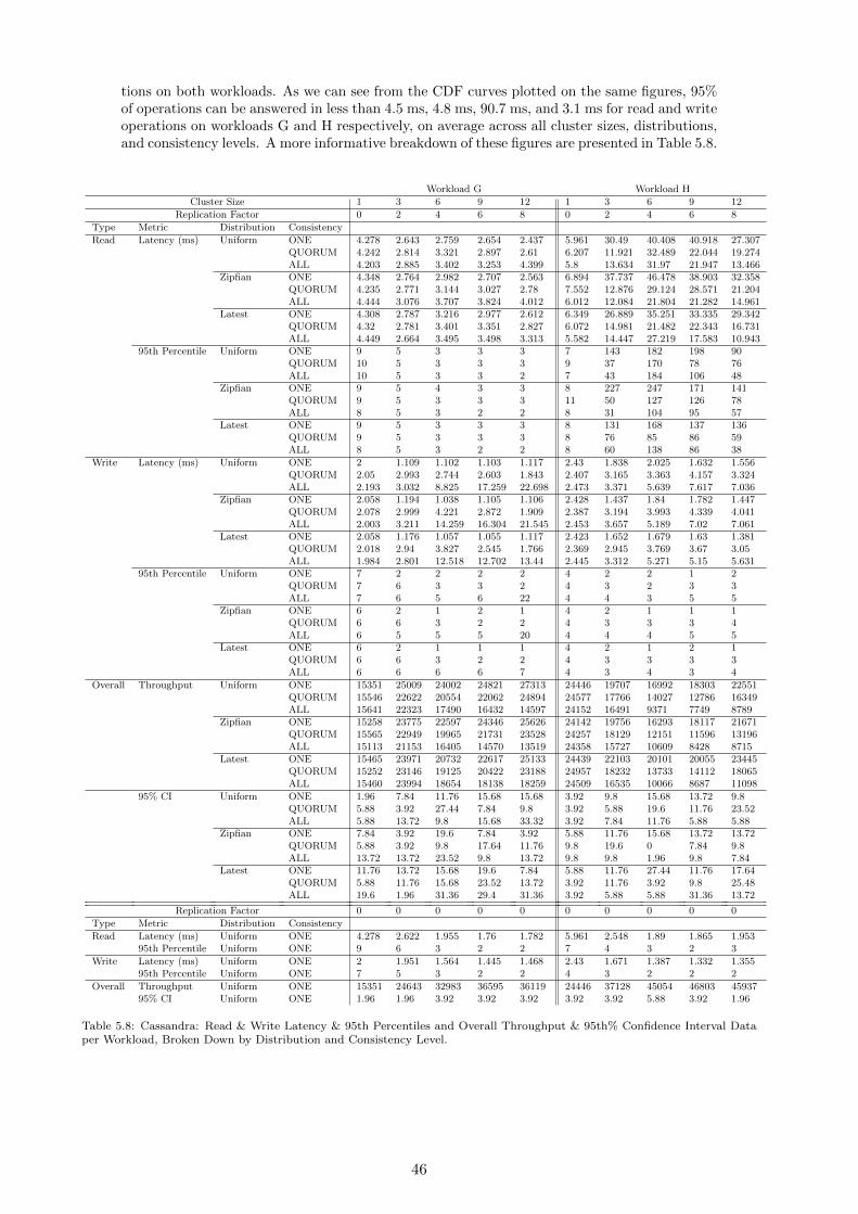
tions on both workloads. As we can see from the CDF curves plotted on the same figures, 95%of operations can be answered in less than 4.5 ms, 4.8 ms, 90.7 ms, and 3.1 ms for read and writeoperations on workloads G and H respectively, on average across all cluster sizes, distributions,and consistency levels. A more informative breakdown of these figures are presented in Table 5.8.


Cluster Size 1 3 6 9 12 1 3 6 9 12









Write Latency (ms) Uniform ONE 2 1.109 1.102 1.103 1.117 2.43 1.838 2.025 1.632 1.556QUORUM 2.05 2.993 2.744 2.603 1.843 2.407 3.165 3.363 4.157 3.324ALL 2.193 3.032 8.825 17.259 22.698 2.473 3.371 5.639 7.617 7.036









95% CI Uniform ONE 1.96 7.84 11.76 15.68 15.68 3.92 9.8 15.68 13.72 9.8QUORUM 5.88 3.92 27.44 7.84 9.8 3.92 5.88 19.6 11.76 23.52ALL 5.88 13.72 9.8 15.68 33.32 3.92 7.84 11.76 5.88 5.88

Zipfian ONE 7.84 3.92 19.6 7.84 3.92 5.88 11.76 15.68 13.72 13.72QUORUM 5.88 3.92 9.8 17.64 11.76 9.8 19.6 0 7.84 9.8ALL 13.72 13.72 23.52 9.8 13.72 9.8 9.8 1.96 9.8 7.84




Read Latency (ms) Uniform ONE 4.278 2.622 1.955 1.76 1.782 5.961 2.548 1.89 1.865 1.95395th Percentile Uniform ONE 9 6 3 2 2 7 4 3 2 3

Write Latency (ms) Uniform ONE 2 1.951 1.564 1.445 1.468 2.43 1.671 1.387 1.332 1.35595th Percentile Uniform ONE 7 5 3 2 2 4 3 2 2 2

Overall Throughput Uniform ONE 15351 24643 32983 36595 36119 24446 37128 45054 46803 4593795% CI Uniform ONE 1.96 1.96 3.92 3.92 3.92 3.92 3.92 5.88 3.92 1.96

Table 5.8: Cassandra: Read & Write Latency & 95th Percentiles and Overall Throughput & 95th% Confidence Interval Dataper Workload, Broken Down by Distribution and Consistency Level.

46


Cluster Size 1 3 6 9 12 1 3 6 9 12






Table 5.9: Cassandra: Percentage Differences In Read & Write Latencies and Overall Throughput Between Distributions foreach Workload and Consistency Level.


Cluster Size 1 3 6 9 12 1 3 6 9 12



Read Latency Uniform ONE 0 0.8 34.1 40.5 31.1 0 169.2 182.1 182.6 173.3QUORUM 0 7.1 51.8 48.8 37.7 0 129.6 178.0 168.8 163.2ALL 0 9.6 54.0 59.6 84.7 0 137.0 177.7 168.7 149.3



Write Latency Uniform ONE 0 55.0 34.7 26.8 27.2 0 9.5 37.4 20.2 13.8QUORUM 0 42.2 54.8 57.2 22.7 0 61.8 83.2 102.9 84.2ALL 0 43.4 139.8 169.1 175.7 0 67.4 121.0 140.5 135.4



Overall Throughput Uniform ONE 0 1.5 31.5 38.3 27.8 0 61.3 90.5 87.5 68.3QUORUM 0 8.6 46.4 49.6 36.8 0 70.5 105.0 114.2 129.6ALL 0 9.9 61.4 76.0 84.9 0 77.0 131.1 143.2 135.8



Table 5.10: Cassandra: Percentage Differences in Read & Write Latencies and Overall Throughput From Baseline Experimentsper Workload, Broken Down by Distribution and Consistency Level.

47













Table 5.11: Cassandra: Percentage Differences In Read & Write Latencies and Overall Throughput Between Workloads foreach Distribution and Consistency Level.

1

10

100

1000

10000

100000

1e+06

1e+07

1e+08

1 10 100 10000

20

40

60

80

100

Num

ber

Of

Op

erat

ions

CD

F(%

)

Latency (ms)


12 nodes

(a)

1

10

100

1000

10000

100000

1e+06

1e+07

1e+08

1 10 100 10000

20

40

60

80

100

Num

ber

Of

Op

erat

ions

CD

F(%

)

Latency (ms)


12 nodes

(b)

1

10

100

1000

10000

100000

1e+06

1e+07

1e+08

1 10 100 10000

20

40

60

80

100N

um

ber

Of

Op

erat

ions

CD

F(%

)

Latency (ms)


12 nodes

(c)

1

10

100

1000

10000

100000

1e+06

1e+07

1e+08

1 10 100 10000

20

40

60

80

100

Num

ber

Of

Op

erat

ions

CD

F(%

)

Latency (ms)


12 nodes

(d)

1

10

100

1000

10000

100000

1e+06

1e+07

1e+08

1 10 100 10000

20

40

60

80

100

Num

ber

Of

Op

erat

ions

CD

F(%

)

Latency (ms)


12 nodes

(e)

1

10

100

1000

10000

100000

1e+06

1e+07

1e+08

1 10 100 10000

20

40

60

80

100

Num

ber

Of

Op

erat

ions

CD

F(%

)

Latency (ms)


12 nodes

(f)

1

10

100

1000

10000

100000

1e+06

1e+07

1e+08

1 10 100 10000

20

40

60

80

100

Num

ber

Of

Op

erat

ions

CD

F(%

)

Latency (ms)


12 nodes

(g)

1

10

100

1000

10000

100000

1e+06

1e+07

1e+08

1 10 100 10000

20

40

60

80

100

Num

ber

Of

Op

erat

ions

CD

F(%

)

Latency (ms)


12 nodes

(h)

1

10

100

1000

10000

100000

1e+06

1e+07

1e+08

1 10 100 10000

20

40

60

80

100

Num

ber

Of

Op

erat

ions

CD

F(%

)

Latency (ms)


12 nodes

(i)

Figure 5.18: Cassandra Workload G Read Latency Histograms: (a) Uniform ONE (b) Uniform QUORUM (c) Uniform ALL(d) Zipfian ONE (e) Zipfian QUORUM (f) Zipfian ALL (g) Latest ONE (h) Latest QUORUM (i) Latest ALL.

48

1

10

100

1000

10000

100000

1e+06

1e+07

1e+08

1 10 100 10000

20

40

60

80

100

Num

ber

Of

Op

erati

ons

CD

F(%

)

Latency (ms)


12 nodes

(a)

1

10

100

1000

10000

100000

1e+06

1e+07

1e+08

1 10 100 10000

20

40

60

80

100

Num

ber

Of

Op

erati

ons

CD

F(%

)

Latency (ms)


12 nodes

(b)

1

10

100

1000

10000

100000

1e+06

1e+07

1e+08

1 10 100 10000

20

40

60

80

100

Num

ber

Of

Op

erati

ons

CD

F(%

)

Latency (ms)


12 nodes

(c)

1

10

100

1000

10000

100000

1e+06

1e+07

1e+08

1 10 100 10000

20

40

60

80

100

Num

ber

Of

Op

erat

ions

CD

F(%

)

Latency (ms)


12 nodes

(d)

1

10

100

1000

10000

100000

1e+06

1e+07

1e+08

1 10 100 10000

20

40

60

80

100

Num

ber

Of

Op

erat

ions

CD

F(%

)

Latency (ms)


12 nodes

(e)

1

10

100

1000

10000

100000

1e+06

1e+07

1e+08

1 10 100 10000

20

40

60

80

100

Num

ber

Of

Op

erat

ions

CD

F(%

)

Latency (ms)


12 nodes

(f)

1

10

100

1000

10000

100000

1e+06

1e+07

1e+08

1 10 100 10000

20

40

60

80

100

Num

ber

Of

Op

erat

ions

CD

F(%

)

Latency (ms)


12 nodes

(g)

1

10

100

1000

10000

100000

1e+06

1e+07

1e+08

1 10 100 10000

20

40

60

80

100

Num

ber

Of

Op

erat

ions

CD

F(%

)

Latency (ms)


12 nodes

(h)

1

10

100

1000

10000

100000

1e+06

1e+07

1e+08

1 10 100 10000

20

40

60

80

100

Num

ber

Of

Op

erat

ions

CD

F(%

)

Latency (ms)


12 nodes

(i)

Figure 5.19: Cassandra Workload G Write Latency Histograms: (a) Uniform ONE (b) Uniform QUORUM (c) Uniform ALL(d) Zipfian ONE (e) Zipfian QUORUM (f) Zipfian ALL (g) Latest ONE (h) Latest QUORUM (i) Latest ALL.

1

10

100

1000

10000

100000

1e+06

1e+07

1e+08

1 10 100 10000

20

40

60

80

100

Num

ber

Of

Op

erat

ions

CD

F(%

)

Latency (ms)


12 nodes

(a)

1

10

100

1000

10000

100000

1e+06

1e+07

1e+08

1 10 100 10000

20

40

60

80

100

Num

ber

Of

Op

erat

ions

CD

F(%

)

Latency (ms)


12 nodes

(b)

1

10

100

1000

10000

100000

1e+06

1e+07

1e+08

1 10 100 10000

20

40

60

80

100

Num

ber

Of

Op

erat

ions

CD

F(%

)

Latency (ms)


12 nodes

(c)

1

10

100

1000

10000

100000

1e+06

1e+07

1e+08

1 10 100 10000

20

40

60

80

100

Num

ber

Of

Op

erat

ions

CD

F(%

)

Latency (ms)


12 nodes

(d)

1

10

100

1000

10000

100000

1e+06

1e+07

1e+08

1 10 100 10000

20

40

60

80

100

Num

ber

Of

Op

erat

ions

CD

F(%

)

Latency (ms)


12 nodes

(e)

1

10

100

1000

10000

100000

1e+06

1e+07

1e+08

1 10 100 10000

20

40

60

80

100

Num

ber

Of

Op

erat

ions

CD

F(%

)

Latency (ms)


12 nodes

(f)

1

10

100

1000

10000

100000

1e+06

1e+07

1e+08

1 10 100 10000

20

40

60

80

100

Num

ber

Of

Op

erat

ions

CD

F(%

)

Latency (ms)


12 nodes

(g)

1

10

100

1000

10000

100000

1e+06

1e+07

1e+08

1 10 100 10000

20

40

60

80

100

Num

ber

Of

Op

erat

ions

CD

F(%

)

Latency (ms)


12 nodes

(h)

1

10

100

1000

10000

100000

1e+06

1e+07

1e+08

1 10 100 10000

20

40

60

80

100

Num

ber

Of

Op

erat

ions

CD

F(%

)

Latency (ms)


12 nodes

(i)

Figure 5.20: Cassandra Workload H Read Latency Histograms: (a) Uniform ONE (b) Uniform QUORUM (c) Uniform ALL(d) Zipfian ONE (e) Zipfian QUORUM (f) Zipfian ALL (g) Latest ONE (h) Latest QUORUM (i) Latest ALL.

49

1

10

100

1000

10000

100000

1e+06

1e+07

1e+08

1 10 100 10000

20

40

60

80

100N

um

ber

Of

Op

erati

ons

CD

F(%

)

Latency (ms)


12 nodes

(a)

1

10

100

1000

10000

100000

1e+06

1e+07

1e+08

1 10 100 10000

20

40

60

80

100

Num

ber

Of

Op

erati

ons

CD

F(%

)

Latency (ms)


12 nodes

(b)

1

10

100

1000

10000

100000

1e+06

1e+07

1e+08

1 10 100 10000

20

40

60

80

100

Num

ber

Of

Op

erati

ons

CD

F(%

)

Latency (ms)


12 nodes

(c)

1

10

100

1000

10000

100000

1e+06

1e+07

1e+08

1 10 100 10000

20

40

60

80

100

Num

ber

Of

Op

erat

ions

CD

F(%

)

Latency (ms)


12 nodes

(d)

1

10

100

1000

10000

100000

1e+06

1e+07

1e+08

1 10 100 10000

20

40

60

80

100

Num

ber

Of

Op

erat

ions

CD

F(%

)

Latency (ms)


12 nodes

(e)

1

10

100

1000

10000

100000

1e+06

1e+07

1e+08

1 10 100 10000

20

40

60

80

100

Num

ber

Of

Op

erat

ions

CD

F(%

)

Latency (ms)


12 nodes

(f)

1

10

100

1000

10000

100000

1e+06

1e+07

1e+08

1 10 100 10000

20

40

60

80

100

Num

ber

Of

Op

erat

ions

CD

F(%

)

Latency (ms)


12 nodes

(g)

1

10

100

1000

10000

100000

1e+06

1e+07

1e+08

1 10 100 10000

20

40

60

80

100

Num

ber

Of

Op

erat

ions

CD

F(%

)Latency (ms)


12 nodes

(h)

1

10

100

1000

10000

100000

1e+06

1e+07

1e+08

1 10 100 10000

20

40

60

80

100

Num

ber

Of

Op

erat

ions

CD

F(%

)

Latency (ms)


12 nodes

(i)

Figure 5.21: Cassandra Workload H Write Latency Histograms: (a) Uniform ONE (b) Uniform QUORUM (c) Uniform ALL(d) Zipfian ONE (e) Zipfian QUORUM (f) Zipfian ALL (g) Latest ONE (h) Latest QUORUM (i) Latest ALL.

50

2000

4000

6000

8000

10000

12000

14000

16000

1 3 6 9 12

Th

rou

gh

pu

t(o

ps/

sec)

Cluster Size

uniformzipfian

latestno-repl

(a)

2000

4000

6000

8000

10000

12000

14000

16000

1 3 6 9 12

Th

rou

gh

pu

t(o

ps/

sec)

Cluster Size

uniformzipfian

latestno-repl

(b)

Figure 5.22: VoltDB: Overall Throughput per Distribution: (a) Workload G (b) Workload H.

400

600

800

1000

1200

1400

1 3 6 9 12

Rea

dL

ate

ncy

(ms)

Cluster Size

uniformzipfian

latestno-repl

(a)

400

600

800

1000

1200

1400

1 3 6 9 12

Rea

dL

ate

ncy

(ms)

Cluster Size

uniformzipfian

latestno-repl

(b)

Figure 5.23: VoltDB: Read Latencies per Distribution: (a) Workload G (b) Workload H.

5.4 VoltDB

As Figure 5.22 illustrates, both workloads report a steady decline in throughput as the clustersize increases before starting to level off, which is an indication of VoltDB’s ability to scale atlarger cluster sizes after a certain overhead of maintaining a small number of nodes. This trendis applicable to both replicated and non-replicated clusters.

On average we see a 45.3%, 40.6%, and 36.3% decrease in throughput for uniform, zipfian,and latest distributions respectively across all cluster sizes with a replication factor greater thanzero compared to non-replicated clusters of equal size for workload G. However, we observegreater decreases in throughput for workload H with 121.4%, 118.3%, and 109.5% decreasesin throughput on average across all cluster sizes with a replication factor greater than zerofor uniform, zipfian, and latest distributions respectively. Details of these metrics are includedin Table 5.12. This considerable difference is due to the synchronous replication model whichVoltDB employs for write operations.

For cluster sizes larger than 3, it’s expected that the throughput would remain constant sincethe number of distinct partitions (i.e. 9) also remain constant. However, the slight decline inperformance is most likely a side effect of the YCSB Client routing all operations to the samenode, requiring additional work on that node’s part to distribute read and write operationsappropriately.

51

0

1000

2000

3000

4000

5000

6000

7000

8000

9000

1 3 6 9 12

Wri

teL

ate

ncy

(ms)

Cluster Size

uniformzipfian

latestno-repl

(a)

0

1000

2000

3000

4000

5000

6000

7000

8000

9000

1 3 6 9 12

Wri

teL

ate

ncy

(ms)

Cluster Size

uniformzipfian

latestno-repl

(b)

Figure 5.24: VoltDB: Write Latencies per Distribution: (a) Workload G (b) Workload H.


Cluster Size 1 3 6 9 12 1 3 6 9 12


Type Metric Distribution

Read Latency Uniform 0 13.3 20.0 51.1 37.6 0 49.6 44.2 39.4 35.2Zipfian 0 10.3 21.1 34.3 36.3 0 36.9 36.4 48.5 39.3Latest 0 9.1 19.5 39.5 38.0 0 14.0 18.5 30.7 30.4

Write Latency Uniform 0 81.2 119.4 161.2 161.3 0 104.2 122.7 143.6 142.9Zipfian 0 81.3 117.4 148.4 153.7 0 91.0 119.9 134.3 144.5Latest 0 76.4 110.2 153.5 160.2 0 75.0 104.7 131.4 141.1

Overall Throughput Uniform 0 19.7 32.4 71.8 57.5 0 95.2 115.9 134.1 140.5Zipfian 0 16.1 31.8 61.6 53 0 87.6 113.6 129.7 142.1Latest 0 14.7 27.8 55.9 46.6 0 72.1 100.9 126.2 138.8

Table 5.12: VoltDB: Percentage Differences in Read & Write Latencies and Overall Throughput From Baseline Experimentsper Workload, Broken Down by Distribution.

The latency for reads across all cluster sizes and distributions remain fairly similar betweenworkloads and in comparison to non-replicated clusters of equal size, as illustrated in Figure5.23. We observe a 22%, and 28.2% increase in read latencies on average across all clustersizes and distributions on workload G, and H respectively compared to non-replicated clustersof equal size. This suggests that reads remain consistently available as the cluster size andreplication factor increases.

However, we observe stark contrasts in read latencies in workload H which consists of only5% read operations compared to workload G on smaller cluster sizes. In order to gain insightinto this observation, additional experiments where conducted to illustrate the impact of work-load composition on read latencies on a single node cluster. The results of these experimentsare illustrated in Table 5.13. We can clearly see that as the percentage of read operations in aworkload increases the latency decreases and subsequently throughput increases almost propor-tionally. For example, a 15% increase in the number of read operations in a workload from 5 to15% corresponds to a 12% decrease in latency and 18% increase in throughput.

The cause of this phenomenon is likely that the large number of (more expensive) writeoperations in the workload impact the availability of a single node cluster for subsequent readoperations. Since all data is located on a single node with 6 partitions, each of which is singlethreaded, the latency for reads is therefore bound by the latency of preceding writes which aremore frequent and take longer to process due to synchronous replication. The reason latencyand throughput measurements start to improve as the cluster size increases is likely due to databeing spread across more servers, with less contention for single-threaded access.

The latency for write operations across all cluster sizes and distributions is considerablyhigher in comparison to non-replicated clusters of equal size, as illustrated in Figure 5.24. Weobserve a 133.1%, and 110.3% increase in write latencies on average across all cluster sizes anddistributions on workload G and H respectively compared to non-replicated clusters of equalsize. It’s interesting however that the percentage difference as the cluster increases from 9 to12 nodes, increases only by 3.7% and 6% for workload G and H respectively. This contrasts toan average increase in percentage difference to non-replicated clusters of 51.7% and 45.6% forworkload G and H respectively each time the cluster grows by 3 additional nodes (until a total

52

% Reads In Workload Latency (ms) Throughput (ops/sec)

5 1.262 570620 1.122 686540 0.859 887580 0.580 1248995 0.525 15216100 0.416 19076

Table 5.13: VoltDB: Percentage of Workload Reads Impact on Read Latency and Overall Throughput.

cluster size of 9). This suggests that the availability for write operations is increasingly affectedon smaller cluster sizes, but potentially stable on larger clusters. A possible explanation forthis is related to the synchronous replication model affecting performance as more replicas areadded, which appears to be amortized on larger clusters due to horizontal scalability.

We also notice the impact synchronous replication has on workload G which consists of only5% write operations. An average increase in write latencies of 127% is observed compared tonon-replicated clusters across all cluster sizes (greater than 1) and distributions. This comparessimilarly to an average increase in write latencies of 121.3% in workload H. This suggests theavailability of the cluster for write operations is affected consistently and independently of theunderlying workload composition within a cluster with a replication factor greater than zero.

Since the total number of partitions available in each cluster is not an integral multiple ofthe cluster size, a single host is likely to store more than 1 copy of the same data partition. Thiswould result in larger latencies due to increased contention when writing to the same commandlog and snapshotting to the same disk, a known performance bottleneck [38]. Throughputswould also be lower since all client invocations are synchronous.

Figures 5.27, 5.28, 5.29, and 5.30 illustrate the latency histograms for read and write op-erations on both workloads. As we can see from the CDF curves plotted on the same figures,95% of operations can be answered in less than 0.5 ms, 1.9 ms, 0.9 ms, and 2.1 ms for readand write operations on workloads G and H respectively, on average across all cluster sizes, anddistributions. A more informative breakdown of these figures is presented in Tables 5.17.

Comparatively, workload G performs consistently better than workload H, reporting a 14.8%increase in throughput on average for non-replicated clusters and 98.6%, 94%, and 83.9% averageincreases in performance for uniform, zipfian, and latest distributions respectively on replicatedclusters. Figure 5.25 demonstrates the comparative performance of both workloads in terms ofthroughput and latencies.

This contrast in performance can be attributed to VoltDB’s handling of reads versus writes.When writing, VoltDB synchronously replicates data to additional nodes therefore incurringlarger impacts on performance. Additionally, command logging and snapshotting is happeningon the same disk which increases disk contention resulting in larger latencies. When readinghowever, since all data is in-memory and no consistency checks are performed between replicas,we observe much higher throughputs at lower latencies.

Read and write latencies show much smaller differences, averaging 13.1% and 27.1% de-creases on average across all replicated cluster sizes and distributions respectively for workloadG compared to workload H. On non-replicated clusters however, the average differences are aslow as 6.8% and 0.1% respectively. These figures are summarized in Table 5.14.

Across both workloads the performance rankings between distributions remain almost per-fectly consistent, regarding throughputs, read latencies, and write latencies. Uniform performsworse that zipfian and latest, with 5% and 8.9% decreases in throughput performance respec-tively for workload G. Larger decreases of 11.3% and 25.2% are observed for workload H. Table5.16 illustrates these findings along with read and write latencies, which follow similar trends.An interesting phenomenon appears in workload H. As the cluster size increases, we observethe performance difference between distributions start to become quite small. This suggests atlarger cluster sizes the difference between each distribution could become negligible.

53

0

2000

4000

6000

8000

10000

12000

14000

16000

18000

1 3 6 9 12

Th

rou

ghp

ut

(op

s/se

c)

Cluster Size



(a)

500

600

700

800

900

1000

1100

1200

1300

1400

1 3 6 9 12

Lat

ency

(ms)

Cluster Size



(b)

0

1000

2000

3000

4000

5000

6000

7000

8000

9000

1 3 6 9 12

Lat

ency

(ms)

Cluster Size



(c)

Figure 5.25: VoltDB: Combined Performance Metrics for each Workload and Distribution: (a) Throughputs (b) Read Latencies(c) Write Latencies.




Read Latency Uniform 82.6 42.4 23.4 5.1 13.0Zipfian 59.4 32.5 14.2 22.0 18.6Latest 32.8 10.6 2.3 1.8 7.8

Write Latency Uniform 68.5 30.4 5.4 41.2 34.6Zipfian 46.3 13.3 6.6 27.5 11.7Latest 18.5 0.4 18.3 44.0 35.0

Overall Throughput Uniform 90.9 90.5 97.2 93.6 120.9Zipfian 66.8 85.7 95.1 96.3 126.0Latest 41.5 71.3 84.0 96.6 126.0



Read Latency Uniform 82.6 5.7 1.3 7.3 15.5Write Latency Uniform 68.5 1.3 10.6 0.7 9.1Overall Throughput Uniform 90.9 13.7 6.5 14.2 24.7

Table 5.14: VoltDB: Percentage Differences In Read & Write Latencies and Overall Throughput Between Workloads for eachDistribution.

Command logging is enabled by default on the Enterprise edition of VoltDB, as such anadditional set of experiments where conducted without command logging or replication to seewhat effect this had on performance and to verify if it followed a similar trend. Figure 5.26indicates that it does follow a similar trend (i.e. a slight downwards trend) and on averageresults in a 72% increase in throughput for workload G, and a 76.7% increase in throughput forworkload H compared to non-replicated clusters of equal size greater than 1 with the defaultsettings enabled. The percentage difference figures per cluster size is indicated in Table 5.15.

0

5000

10000

15000

20000

25000

1 3 6 9 12

Th

rou

ghp

ut

(op

s/se

c)

Cluster Size

uniformzipfianlatest

no-replno-repl or logging

(a)

0

5000

10000

15000

20000

25000

1 3 6 9 12

Th

rou

ghp

ut

(op

s/se

c)

Cluster Size

uniformzipfianlatest

no-replno-repl or logging

(b)

Figure 5.26: VoltDB Overall Throughputs per Distribution and Baseline Experiments with no Command Logging: (a) WorkloadG (b) Workload H.

54

Throughput % Difference

Cluster Size Workload G Workload H

1 - -3 63.806 67.46056 78.3771 76.39299 77.0599 80.815412 68.8411 81.8932

avg: 72.02102 76.6405

Table 5.15: VoltDB: Overall Throughput Differences Between No-Replication and No-Replication or Command Logging Ex-periments.


Cluster Size 1 3 6 9 12 1 3 6 9 12


Type Metric Distribution avg avg

Read Latency Uniform vs Zipfian 4.1 3.1 1.1 17.5 1.3 5.4 30.5 13.3 8.2 9.6 4.3 13.2Uniform vs Latest 4.7 4.3 0.5 12.2 0.4 4.4 57.8 36.2 26.2 9.0 4.9 26.8

Write Latency Uniform vs Zipfian 8.4 0.1 3.1 31.8 20.0 12.7 32.3 17.3 4.4 18.0 3.3 15.0Uniform vs Latest 7.4 5.7 13.6 20.1 3.1 10.0 58.5 36.3 26.4 23.1 3.5 29.6

Overall Throughput Uniform vs Zipfian 4.2 3.7 0.6 11.4 5.0 5.0 32.4 9.6 3.3 7.9 3.3 11.3Uniform vs Latest 5.5 5.1 4.7 17.6 11.6 8.9 59.7 27.9 21.2 13.8 3.3 25.2

Table 5.16: VoltDB: Percentage Differences In Read & Write Latencies and Overall Throughput Between Distributions for eachWorkload.


Cluster Size 1 3 6 9 12 1 3 6 9 12



Read Latency (ms) Uniform 0.524 0.696 0.917 1.314 1.068 1.262 1.07 1.16 1.249 1.217Zipfian 0.503 0.675 0.927 1.102 1.054 0.928 0.937 1.069 1.375 1.27Latest 0.5 0.667 0.912 1.163 1.072 0.696 0.742 0.891 1.142 1.159

95th Percentile Uniform 0 0 1 1 0 1 1 1 1 1Zipfian 0 0 1 1 1 1 1 1 1 1Latest 0 1 1 1 0 0 0 1 1 1

Write Latency (ms) Uniform 0.685 1.655 3.592 8.348 7.914 1.399 2.249 3.404 5.498 5.577Zipfian 0.63 1.656 3.483 6.055 6.476 1.01 1.891 3.259 4.591 5.763Latest 0.636 1.564 3.134 6.82 7.669 0.766 1.558 2.609 4.36 5.384

95th Percentile Uniform 0 1 2 3 4 1 2 2 3 3Zipfian 0 1 2 2 4 1 1 2 3 4Latest 0 1 2 3 3 0 1 2 3 3

Overall Throughput Uniform 15216 10690 7577 4794 6087 5706 4031 2622 1737 1501Zipfian 15862 11089 7625 5375 6398 7916 4438 2711 1880 1452Latest 16080 11249 7942 5719 6838 10558 5338 3244 1995 1552

95% CI Uniform 9.80 3.92 1.96 1.96 13.72 0 15.68 11.76 11.76 1.96Zipfian 9.80 5.88 5.88 9.80 13.72 5.88 7.84 11.76 5.88 1.96Latest 13.72 9.80 9.80 11.76 21.56 9.80 5.88 7.84 5.88 1.96



Read Latency (ms) Uniform 0.524 0.609 0.75 0.779 0.73 1.262 0.645 0.74 0.838 0.85395th Percentile Uniform 0 0 1 1 1 1 0 1 1 1

Write Latency (ms) Uniform 0.685 0.699 0.907 0.897 0.848 1.399 0.708 0.816 0.903 0.92995th Percentile Uniform 0 1 1 1 1 1 0 1 1 1

Overall Throughput Uniform 15216 13029 10507 10161 10998 5706 11353 9845 8814 858495% CI Uniform 9.8 9.80 5.88 5.88 11.76 0 7.84 5.88 1.96 1.96

Table 5.17: VoltDB: Read & Write Latency & 95th Percentiles and Overall Throughput & 95th% Confidence Interval Data perWorkload, Broken Down by Distribution.

55

1

10

100

1000

10000

100000

1e+06

1e+07

1 10 100 10000

20

40

60

80

100N

um

ber

Of

Op

erati

ons

CD

F(%

)

Latency (ms)


12 nodes

(a)

1

10

100

1000

10000

100000

1e+06

1e+07

1 10 100 10000

20

40

60

80

100

Num

ber

Of

Op

erati

ons

CD

F(%

)

Latency (ms)


12 nodes

(b)

1

10

100

1000

10000

100000

1e+06

1e+07

1 10 100 10000

20

40

60

80

100

Num

ber

Of

Op

erat

ions

CD

F(%

)

Latency (ms)


12 nodes

(c)

Figure 5.27: VoltDB Workload G Read Latency Histograms: (a) Uniform (b) Zipfian (c) Latest.

1

10

100

1000

10000

100000

1e+06

1e+07

1 10 100 10000

20

40

60

80

100

Num

ber

Of

Op

erat

ions

CD

F(%

)

Latency (ms)


12 nodes

(a)

1

10

100

1000

10000

100000

1e+06

1e+07

1 10 100 10000

20

40

60

80

100

Num

ber

Of

Op

erat

ions

CD

F(%

)

Latency (ms)


12 nodes

(b)

1

10

100

1000

10000

100000

1e+06

1e+07

1 10 100 10000

20

40

60

80

100

Num

ber

Of

Op

erat

ions

CD

F(%

)

Latency (ms)


12 nodes

(c)

Figure 5.28: VoltDB Workload G Write Latency Histograms: (a) Uniform (b) Zipfian (c) Latest.

1

10

100

1000

10000

100000

1e+06

1e+07

1 10 100 10000

20

40

60

80

100

Num

ber

Of

Op

erat

ions

CD

F(%

)

Latency (ms)


12 nodes

(a)

1

10

100

1000

10000

100000

1e+06

1e+07

1 10 100 10000

20

40

60

80

100

Num

ber

Of

Op

erat

ions

CD

F(%

)

Latency (ms)


12 nodes

(b)

1

10

100

1000

10000

100000

1e+06

1e+07

1 10 100 10000

20

40

60

80

100

Num

ber

Of

Op

erat

ions

CD

F(%

)

Latency (ms)


12 nodes

(c)

Figure 5.29: VoltDB Workload H Read Latency Histograms: (a) Uniform (b) Zipfian (c) Latest.

1

10

100

1000

10000

100000

1e+06

1e+07

1 10 100 10000

20

40

60

80

100

Num

ber

Of

Op

erat

ions

CD

F(%

)

Latency (ms)


12 nodes

(a)

1

10

100

1000

10000

100000

1e+06

1e+07

1 10 100 10000

20

40

60

80

100

Num

ber

Of

Op

erat

ions

CD

F(%

)

Latency (ms)


12 nodes

(b)

1

10

100

1000

10000

100000

1e+06

1e+07

1 10 100 10000

20

40

60

80

100

Num

ber

Of

Op

erat

ions

CD

F(%

)

Latency (ms)


12 nodes

(c)

Figure 5.30: VoltDB Workload H Write Latency Histograms: (a) Uniform (b) Zipfian (c) Latest.

56

5.5 Comparative Analysis

While not the primary focus of this study, there are a number of comparisons that can be drawnbetween each data store. Based on the data and material presented so far, this section looks atseveral key things including: which data store offers the highest throughput and lowest latencies;what impact did each distribution have relative to each data store; and finally, which replicationmodel had the least impact on baseline performances.

Redis, which averages 35298 ops/sec across all cluster sizes, consistency levels, and distribu-tions outperforms MongoDB (averaging 21230 ops/sec) by 49.8%. MongoDB is only marginallybetter than Cassandra (which averages 20184 ops/sec) by 5.1%. Finally Cassandra outperformsVoltDB which averages 9236 ops/sec by 74.4% on the read-heavy workload (G).

A similar trend is observable for workload H which is write dominated, however the greatestdifference is that Cassandra outperforms MongoDB by 72.5%. This stark contrast is a clear indi-cation of Cassandra’s write optimized architecture. Figures 5.31a and 5.32a illustrate how eachdata store performs relatively as the cluster size increases, for workload G and H respectively.

Overall, Redis outperforms all other data stores due its simplistic nature. Additional replicasdo not have an impact on performance, and in-memory updates to a single hash table are quick,constant time operations. Additionally, varying consistency levels (due to a lack of supporta-bility) and distributions have no impact on performance. VoltDB is the worst performer, mostlikely as a result of its strictly consistent architecture.

If we consider latencies, Redis again outperforms the other data stores by a large margin.Read latencies are 115.1% and 135% lower for workload G and H respectively compared tothe next performant data store: VoltDB, with 174.9% and 163% lower write latencies also. Asimilar trend between MongoDB and Cassandra is observable for read and writes latencies as wesaw for throughputs. MongoDB’s read latencies are lower that Cassandra’s (5.9% and 136.2%for workload G and H respectively). However, Cassandra’s write latencies are much lower thanMongoDB’s (19.3% and 102% for workload G and H respectively).

The fact that Redis and VoltDB have lower latencies is expected due to the fact they areboth in-memory data stores. Again, Redis’s hash table data structure results in lower latenciessince they are constant time operations. Figures 5.31b and 5.32b illustrate how each data store’sread latencies differ as the cluster size increases, for workload G and H respectively. Similarly,Figures 5.31c and 5.32c illustrate how each data store’s write latencies differ as the cluster sizeincreases, for workload G and H respectively.

5000

10000

15000

20000

25000

30000

35000

40000

1 3 6 9 12

Thro

ugh

put

(ops/

sec)

Cluster Size

RedisVoltDB

MongoDBCassandra

(a)

0

5000

10000

15000

20000

25000

30000

35000

1 3 6 9 12

Lat

ency

(ms)

Cluster Size

RedisVoltDB

MongoDBCassandra

(b)

0

5000

10000

15000

20000

1 3 6 9 12

Lat

ency

(ms)

Cluster Size

RedisVoltDB

MongoDBCassandra

(c)

Figure 5.31: Comparison of Data Stores averaged across all distributions and consistency levels for Workload G: (a) OverallThroughput (b) Read Latency (c) Write Latency.

57

5000

10000

15000

20000

25000

30000

35000

40000

1 3 6 9 12

Thro

ughput

(ops/

sec)

Cluster Size

RedisVoltDB

MongoDBCassandra

(a)

0

5000

10000

15000

20000

25000

30000

35000

1 3 6 9 12

Late

ncy

(ms)

Cluster Size

RedisVoltDB

MongoDBCassandra

(b)

0

5000

10000

15000

20000

1 3 6 9 12

Late

ncy

(ms)

Cluster Size

RedisVoltDB

MongoDBCassandra

(c)

Figure 5.32: Comparison of Data Stores averaged across all distributions and consistency levels for Workload H: (a) OverallThroughput (b) Read Latency (c) Write Latency.

In workload G, all data stores demonstrate better performances with the latest distribution,except Cassandra which performs best with the uniform distribution. Redis consistently out-performs MongoDB on all distributions followed by Cassandra then VoltDB. Again, the onlyexception to this observation is that Cassandra has better throughputs than MongoDB with theuniform distribution. Cassandra’s better performance on read-heavy workloads with a uniformdistribution is likely a result of a strong correlation between how the YCSB Client selects a nodeto route requests to uniformly at random. This would spread the requests more evenly acrossthe cluster. Whereas the latest distribution would force the same set of nodes to constantlyhandle operations, causing a backlog of read-repairs to build up. When accessed with the latestdistribution, Redis is 1.5 times more performant than MongoDB, which is only 1.1 times moreperformant than Cassandra, which is 2.1 times more performant than VoltDB.

The latest distribution once again in workload H outperforms all other distributions on av-erage across all cluster sizes and consistency levels, followed by zipfian, except for Cassandrawhich performs second best with the uniform distribution. When all data stores are accessedwith the latest distribution, Redis is 1.4 times more performant than Cassandra which is 2times better than MongoDB which is again 2 time better than VoltDB. The reason we observelarger contrasts in relative performance compared to workload G, is because Cassandra is writeoptimized, MongoDB performs consistency checks at write time, and VoltDB synchronouslyreplicates data to replicas therefore incurring the largest impact on performance.

If we consider the impact replication has on clusters of equal size and compare two differentreplication strategies i.e. the multi-master model used by Cassandra, and the replica set modelused by MongoDB. We can observe that apart from the exception of consistency level ONE onworkload G, MongoDB’s replica set replication model has less of an impact on throughput per-formance than Cassandra’s multi-master replication model compared to non-replicated clusters.Cassandra’s replication model accounts for a 41.1%, and 98% throughput performance degrada-tion on all consistency levels and distributions, averaged across all replicated clusters sizes forworkload G and H respectively. Whereas MongoDB’s replication model only accounts for 33%and 52% degradation’s in throughput performance for workload G and H respectively. Figures5.33a and 5.34a illustrate how each replication strategy performs relatively and in relation tobase line performances as the cluster size increases, for workload G and H respectively.

Both read and write latencies are more adversely affected with Cassandra’s multi-slave repli-cation model compared to non-replicated clusters of equal size. We observe 40.5% and 72.9%increases in read and write latencies for workload G. More prominently however, we observe164.4% and 71.3% increases in read and write latencies on workload H. More modest increasesin latencies are achieved for MongoDB’s replica set replication model compared to non-replicatedclusters of equal size. We observe 33.8% and 30.3% increases in read and write latencies forworkload G and similarly 21.4% and 42.1% increases in read and write latencies respectivelyfor workload H. This suggests that a master-slave replication model has less of an effect onclusters than a multi-master model. Figures 5.33b and 5.34b illustrate how each replicationstrategy’s read latencies differ as the cluster size increases, for workload G and H respectivelyand compared to base line performances. Similarly, Figures 5.33c and 5.34c illustrate how eachreplication strategy’s write latencies differ as the cluster size increases, for workload G and Hrespectively and compared to base line performances.

58

5000

10000

15000

20000

25000

30000

35000

40000

1 3 6 9 12

Thro

ughput

(ops/

sec)

Cluster Size

MongoDBMongoDB no-repl

CassandraCassandra no-repl

(a)

0

5000

10000

15000

20000

25000

30000

35000

1 3 6 9 12

Late

ncy

(ms)

Cluster Size



(b)

0

5000

10000

15000

20000

1 3 6 9 12

Lat

ency

(ms)

Cluster Size



(c)

Figure 5.33: Comparison of Replication strategies: Multi-Master (Cassandra) and Replica Sets (MongoDB), averaged acrossall distributions and consistency levels for Workload G: (a) Overall Throughput (b) Read Latency (c) Write Latency.

0

5000

10000

15000

20000

25000

30000

35000

40000

45000

50000

1 3 6 9 12

Thro

ugh

put

(ops/

sec)

Cluster Size



(a)

0

5000

10000

15000

20000

25000

30000

35000

1 3 6 9 12

Lat

ency

(ms)

Cluster Size



(b)

0

5000

10000

15000

20000

1 3 6 9 12

Lat

ency

(ms)

Cluster Size



(c)

Figure 5.34: Comparison of Replication strategies: Multi-Master (Cassandra) and Replica Sets (MongoDB), averaged acrossall distributions and consistency levels for Workload H: (a) Overall Throughput (b) Read Latency (c) Write Latency.

59

6 Conclusion

This study looked at performance benchmarking replication in four cloud serving NoSQL datastores, focusing specifically on how performance and availability was affected compared to non-replicated clusters of equal size. The YCSB benchmarking tool was used to evaluate datastores of different categorization and replication models. These include key-value, document,extensible-record and distributed DBMS data stores and different variations of master-slave,and multi-master replication models.

To increase the applicability of this study to real-world use cases, a range of different datadistributions (uniform, zipfian, and latest) were explored along with three levels of tunableconsistency: ONE, QUORUM, and ALL, and two different workloads: one read-heavy and onewrite-heavy.

6.1 Benchmarking Results

Considering the extensive number and breadth of experiments conducted in this study, thereare a number of key observations that have been made, the most significant of which are sum-marized below.

Redis:

• Read operations remain highly and consistently available in replicated clusters. Increasingthe replication factor greater than 2 results in consistent performance metrics and noadditional benefit for read operations.

• The availability for write operations are affected on average by 19.2% each time the clustersize is increased with 3 additional replicas.

• There are minimal differences between distributions since Redis keeps all data in memoryon a single master.

• Varying levels of tunable consistency have no impact on performance due to Redis’ lackof consistency guarantees and its efficient implementation.

MongoDB:

• Read heavy workloads outperform write-heavy workloads on average by a considerablemargin: 88.7% across all cluster sizes, distributions and consistency levels.

• Replication has minimal impact on performance relative to non-replicated clusters of equalsize once the overhead of maintaining a small number of shards have been overcome.

• Reads remain highly available (with 10% variance) as the cluster size grows with a constantreplication factor on more than one shard.

• Writes tend to be half as available as reads (20% variance) when the replication factor iskept constant as the cluster size grows.

• Increasing the level of consistency reduces overall performance by increasingly small amounts.Between consistency levels ONE and ALL, a 4.8% and 5.9% drop in throughput for work-load G and H respectively is observed.

• Performance is best when the entire or majority of a working data set can be kept in RAM,as it would be for latest and zipfian distributions.

Cassandra:

• Write latencies are lower than read latencies, however throughputs follow an opposite trend(35.9% decrease on average for writes) on replicated clusters.

• Cassandra is scalable at the cost of maintaining a lower level of consistency. 65.6% and74.6% degradations are observed between consistency levels ONE and ALL for workloadG and H respectively, on average across all replicated cluster sizes and distributions.

• Stricter consistency levels have a greater impact (9%) on write-heavy workloads than onread-heavy workloads.

• The availability of a replicated cluster for read operations is considerably impacted by thenumber of write operations than are present in a workload. Increases in latencies of 150%are observed on average across all cluster sizes, consistency levels, and distributions whenincreasing the write portion of a workload by 90%.

60

• Uniform distributions are 4.2% more performant on read-heavy workloads. However, thelatest distribution is 7.1% more performant in write-heavy workloads.

VoltDB:

• VoltDB appears to scale well at cluster sizes larger than 9 and a replication factor of 6 dueto an observable levelling off of performance degradation.

• With replication, the availability of the cluster for write operations is affected consistentlyand independently of the underlying workload composition.

• Read operations remain consistently available as the cluster size and replication factorincreases, suffering only minor degradations compared to non-replicated cluster of equalsize when the read portion of a workload forms the majority.

• When the percentage of write operations in a workload increases, the availability of thecluster for read operations is proportionally affected on single node clusters.

• Reads are more performant than writes which demonstrate greater degradation’s in per-formance compared to non-replicated clusters of equal size.

• Variable distributions demonstrate minimal differences and on larger cluster sizes the dif-ferences are almost negligible.

• Disabling command logging results in approximately a 75% increase in performance.

The variety of data stores included in this study enabled basic comparisons to be drawnbetween each data store type and replication model.

In-memory data stores (Redis & VoltDB) have much lower latencies than data stores that relyon disk-bound operations (MongoDB & Cassandra) for both read and write-heavy workloads.For example, Redis had 172% and 187.4% lower read and write latencies compared to MongoDBfor workload G and H respectively.

Redis, a key-value store, recorded the highest throughputs seemingly due to its simpler un-derlying implementation i.e. hash tables. However, due to lack of supportability in Redis;varying replication factors, consistency levels, and data distributions didn’t have the same im-pact as on other data stores. Redis was 49.8% and 40.6% more performant than the second bestdata stores (MongoDB & Cassandra) on workload G and H respectively. Distributed DBMSsare least performant, likely as a result of being fully ACID compliant. VoltDB was 117% and149% less performant than Redis for workload G and H respectively.

Master-slave type replication models, as exhibited by Redis and MongoDB tend to reducethe impact replication has on a non-replicated cluster of equal size compared to multi-masterreplication models exhibited by Cassandra and VoltDB. It was observed that MongoDB’s repli-cation model accounted for 8.1% and 46% less impact on performance compared to Cassandraon non-replicated clusters. This is a result of each master and slave being responsible for a singledata partition leading to reduced access contention compared to the multi-master models usedby Cassandra and VoltDB which contain more than one unique partition on a single server.

6.2 Limitations

Access to limited resources meant that the cluster and replication configurations which couldbe set up were not as exhaustive as they could have been. It would be informative to be able toevaluate the effect larger data sets and cluster sizes had on each system. With recent advancesin flash memory, it would be instructive to observe the impact SSDs have on performance dueto their lower access times and reduced latency compared to traditional hard disk drives. Flashmemory is quickly becoming an industry standard for persistent data storage.

The instability of the private cloud environment meant that a lot of repeats of experimentshad to be conducted which consumed a large amount of time. Surveying the 95th percentilefigures and observing the performance metrics achieved in some of the benchmarks highlightedin the literature, suggests that there is room for improvement, which a more stable cloud envi-ronment could have greatly helped with.

Due to the poor client support for Redis Cluster, a feature that remained in beta testingthroughout this project, which offers much more sophisticated cluster configurations comparableto the other data stores under test in this study, unfortunately was not implemented. Should

61

the client-side support for Redis Cluster improve over the coming software releases, it would behighly informative to run similar nontrivial replication experiments against it.

It was unfortunate that a warm-up stage could not be implemented for the customizedVoltDB YCSB client driver within the time constraints of this study. As a result, the perfor-mance metrics for VoltDB are slightly skewed compared to the others. Analysis of the resultshowever, suggest that adding a warm-up stage would not affect the relative performance be-tween data stores. However, the poor results observable in this study contradict the VoltDBliterature and benchmark conducted in [59]. As such, futher optimizations and experimentationwould be beneficial.

This study does not account for the performance optimizations and additional features avail-able in the most recent version of Cassandra due to an incompatible YCSB client driver. Sub-sequently, the results gathered in this study are only applicable to a portion of current industryimplementations and offers limited guidance for future implementations.

6.3 Future Work

Initially, the current limitations would be addressed as summarized below:

• Update the Cassandra YCSB client driver to support Cassandra 2.0, subsequently releas-ing this code back into the community. This will more realistically aid future industryimplementations of Cassandra.

• Add a warm-up stage to the VoltDB YCSB client driver and identify further optimiza-tions to increase performance in line with existing literature and VoltDB benchmarks andincrease the comparable strength with other data stores.

• Deploy and benchmark a stable release of Redis Cluster with similar replication experi-ments to MongoDB.

• Conduct a similar benchmark on Amazon’s EC2 cloud, extending experiments to includelarger data set and cluster sizes while making use of SSDs to better reflect industry stan-dard deployments.

• Consider resource usage in analysis in order to support the conclusions derived about theunderlying activity of each data store.

• Perform more in-depth analysis on the comparable nature of each data store.

Only two out of the four important measures highlighted in Cooper et al.’s original YCSBpaper [14] for adding a new benchmarking tier for replication were explored in this study. Inorder to address all of these measures and work towards implementing a complete replicationtier in YCSB, it would be essential to continue pursuing these measures in future iterations ofthis work. These measures are:

• Geo-replication: An industry recommended solution to ensure fault tolerance in the faceof network partitions and entire data center failures. There are important implicationsregarding geo-replication which are likely to affect performance due to the increase inround trip time for communicating and transferring data between geographically dispersedcluster nodes. In addition, some data stores optimize replication for within a single datacenter or between nearby data centers, while others are optimized for globally distributeddata centers [14].

• Data consistency: This measure would evaluate the impact replication had on the con-sistency of data, including metrics on what proportion of the data is stale and by how much.

To aid and encourage future performance modelling and additional studies investigatingreplication in NoSQL data stores, all raw YCSB log data collected in this study is publiclyavailable35. The most immediate future studies could involve performance modelling Redis,MongoDB, and VoltDB.

35http://www.doc.ic.ac.uk/~gh413/YCSB/

62

References

[1] Accenture. http://www.accenture.com/.

[2] Aerospike. http://www.aerospike.com/.

[3] AstraZeneca. http://www.astrazeneca.co.uk/home.

[4] Falko Bause. Queueing petri nets-a formalism for the combined qualitative and quantita-tive analysis of systems. In Petri Nets and Performance Models, 1993. Proceedings., 5thInternational Workshop on, pages 14–23. IEEE, 1993.

[5] TCP Benchmarks. http://www.tpc.org/information/benchmarks.asp. Last Accessed:2014.07.19.

[6] Carsten Binnig, Donald Kossmann, Tim Kraska, and Simon Loesing. How is the weathertomorrow?: towards a benchmark for the cloud. In Proceedings of the Second InternationalWorkshop on Testing Database Systems, page 9. ACM, 2009.

[7] Dhruba Borthakur. Facebook has the world’s largest hadoop cluster! http://hadoopblog.

blogspot.co.uk/2010/05/facebook-has-worlds-largest-hadoop.html, May 2010.Last Accessed: 2014.07.19.

[8] Eric A Brewer. Towards robust distributed systems. In PODC, page 7, 2000.

[9] Cassandra. http://cassandra.apache.org/.

[10] Rick Cattell. Scalable sql and nosql data stores. ACM SIGMOD Record, 39(4):12–27, 2011.

[11] Fay Chang, Jeffrey Dean, Sanjay Ghemawat, Wilson C Hsieh, Deborah A Wallach, MikeBurrows, Tushar Chandra, Andrew Fikes, and Robert E Gruber. Bigtable: A distributedstorage system for structured data. ACM Transactions on Computer Systems (TOCS),26(2):4, 2008.

[12] Kristina Chodorow. MongoDB: the definitive guide. ” O’Reilly Media, Inc.”, 2013.

[13] Brian F Cooper, Raghu Ramakrishnan, Utkarsh Srivastava, Adam Silberstein, Philip Bo-hannon, Hans-Arno Jacobsen, Nick Puz, Daniel Weaver, and Ramana Yerneni. Pnuts:Yahoo!’s hosted data serving platform. Proceedings of the VLDB Endowment, 1(2):1277–1288, 2008.

[14] Brian F Cooper, Adam Silberstein, Erwin Tam, Raghu Ramakrishnan, and Russell Sears.Benchmarking cloud serving systems with ycsb. In Proceedings of the 1st ACM symposiumon Cloud computing, pages 143–154. ACM, 2010.

[15] Datastax Coperation. Benchmarking top nosql databases. a performance comparison forarchitects and it managers. 2013.

[16] Couchbase. http://www.couchbase.com/.

[17] Coursera. https://www.coursera.org/.

[18] Datastax. About datastax. http://www.datastax.com/company.

[19] Jeffrey Dean and Sanjay Ghemawat. Mapreduce: simplified data processing on large clus-ters. Communications of the ACM, 51(1):107–113, 2008.

[20] Elif Dede, Bedri Sendir, Pinar Kuzlu, Jessica Hartog, and Madhusudhan Govindaraju.An evaluation of cassandra for hadoop. In Cloud Computing (CLOUD), 2013 IEEE SixthInternational Conference on, pages 494–501. IEEE, 2013.

[21] David J DeWitt. The wisconsin benchmark: Past, present, and future., 1993.

[22] Diomin and Grigorchuk: Altoros Systems Inc. Benchmarking couchbase server for interac-tive applications. http://www.altoros.com/, 2013.

[23] Eventribe. https://www.eventbrite.co.uk.

[24] Daniel Ford, Francois Labelle, Florentina I Popovici, Murray Stokely, Van-Anh Truong,Luiz Barroso, Carrie Grimes, and Sean Quinlan. Availability in globally distributed storagesystems. In OSDI, pages 61–74, 2010.

[25] A. Gandini, M. Gribaudo, W. J. Knottenbelt, R. Osman, and P. Piazzolla. Performanceanalysis of nosql databases. In 11th European Performance Engineering Workshop (EPEW2014), 2014.

[26] Alvaro Garcıa-Recuero, Sergio Esteves, and Luıs Veiga. Quality-of-data for consistencylevels in geo-replicated cloud data stores. In Cloud Computing Technology and Science(CloudCom), 2013 IEEE 5th International Conference on, volume 1, pages 164–170. IEEE,2013.

63

[27] Seth Gilbert and Nancy Lynch. Brewer’s conjecture and the feasibility of consistent, avail-able, partition-tolerant web services. ACM SIGACT News, 33(2):51–59, 2002.

[28] Github. https://github.com/.

[29] Apache Hadoop. http://hadoop.apache.org.

[30] Stavros Harizopoulos, Daniel J Abadi, Samuel Madden, and Michael Stonebraker. Oltpthrough the looking glass, and what we found there. In Proceedings of the 2008 ACMSIGMOD international conference on Management of data, pages 981–992. ACM, 2008.

[31] HBase. http://hbase.apache.org/.

[32] Eben Hewitt. Cassandra: the definitive guide. O’Reilly Media Inc., 2010.

[33] MongoDB Inc. Mongodb manual: Replication. http://docs.mongodb.org/manual/

replication/.

[34] MongoDB Inc. Mongodb manual: Sharded cluster config servers. http://docs.mongodb.org/manual/core/sharded-cluster-config-servers/.

[35] MongoDB Inc. Mongodb manual: Sharded collection balancer. http://docs.mongodb.

org/manual/core/sharding-balancing/.

[36] MongoDB Inc. Mongodb manual: Sharding. http://docs.mongodb.org/manual/

sharding/.

[37] VoltDB Inc. Voltdb technical overview. http://voltdb.com/downloads/datasheets_

collateral/technical_overview.pdf, 2010. Retrived 2014.07.16.

[38] VoltDB Inc. Using voltdb. https://voltdb.com/downloads/documentation/

UsingVoltDB.pdf, 2014.

[39] Sakura Internet. http://www.sakura.ne.jp.

[40] Robert Kallman, Hideaki Kimura, Jonathan Natkins, Andrew Pavlo, Alexander Rasin,Stanley Zdonik, Evan PC Jones, Samuel Madden, Michael Stonebraker, Yang Zhang, et al.H-store: a high-performance, distributed main memory transaction processing system. Pro-ceedings of the VLDB Endowment, 1(2):1496–1499, 2008.

[41] Avinash Lakshman and Prashant Malik. Cassandra: a decentralized structured storagesystem. ACM SIGOPS Operating Systems Review, 44(2):35–40, 2010.

[42] Greg Linden. Make data useful. Presentation, Amazon, November, 2006.

[43] LinkedIn. https://www.linkedin.com/.

[44] Matt Massie, Bernard Li, Brad Nicholes, Vladimir Vuksan, Robert Alexander, Jeff Buch-binder, Frederiko Costa, Alex Dean, Dave Josephsen, Peter Phaal, et al. Monitoring withGanglia. O’Reilly Media, Inc, 2012.

[45] MongoDB. http://www.mongodb.org/.

[46] Steffen Muller, David Bermbach, Stefan Tai, and Frank Pallas. Benchmarking the perfor-mance impact of transport layer security in cloud database systems.

[47] Nelubin and Engber: Thumbtack Technology Inc. Nosql failover characteristics: Aerospike,cassandra, couchbase, mongodb. http://www.thumbtack.net/, 2013.

[48] Nelubin and Engber: Thumbtack Technology Inc. Ultra-high performance nosql bench-marking. http://www.thumbtack.net/, 2013.

[49] R. Osman and P. Piazzolla. Modelling replication in nosql datastores. In 11th InternationalConference on Quantitative Evaluation of Systems (QEST), 2014.

[50] Tim Oreilly. Web 2.0: compact definition. Message posted to http://radar. oreilly.com/archives/2005/10/web 20 compact definition. html, 2005. Retrived 2014.07.07.

[51] Swapnil Patil, Milo Polte, Kai Ren, Wittawat Tantisiriroj, Lin Xiao, Julio Lopez, GarthGibson, Adam Fuchs, and Billie Rinaldi. Ycsb++: benchmarking and performance debug-ging advanced features in scalable table stores. In Proceedings of the 2nd ACM Symposiumon Cloud Computing, page 9. ACM, 2011.

[52] Andrew Pavlo, Erik Paulson, Alexander Rasin, Daniel J Abadi, David J DeWitt, SamuelMadden, and Michael Stonebraker. A comparison of approaches to large-scale data analysis.In Proceedings of the 2009 ACM SIGMOD International Conference on Management ofdata, pages 165–178. ACM, 2009.

64

[53] Pouria Pirzadeh, Junichi Tatemura, and Hakan Hacigumus. Performance evaluation ofrange queries in key value stores. In Parallel and Distributed Processing Workshops andPhd Forum (IPDPSW), 2011 IEEE International Symposium on, pages 1092–1101. IEEE,2011.

[54] Pivotal. http://www.pivotal.io/.

[55] Alexander Pokluda and Wei Sun. Benchmarking failover characteristics of large-scale datastorage applications: Cassandra and voldemort.

[56] Tilmann Rabl, Sergio Gomez-Villamor, Mohammad Sadoghi, Victor Muntes-Mulero, Hans-Arno Jacobsen, and Serge Mankovskii. Solving big data challenges for enterprise applicationperformance management. Proceedings of the VLDB Endowment, 5(12):1724–1735, 2012.

[57] Rackspace. http://www.rackspace.co.uk/.

[58] Redis. http://redis.io/.

[59] Alex Rogers. Voltdb in-memory database achieves best-in-class results, running in thecloud, on the ycsb benchmark. http://tinyurl.com/VoltDB-YCSB, May 2014. Last Ac-cessed: 2014.07.06.

[60] Alex Rogers. Ycsb for voltdb. http://stackoverflow.com/a/23528926/2298888, 2014.Last Accessed: 2014.08.25.

[61] Michael Russo. Redis, from the ground up. http://blog.mjrusso.com/2010/10/17/

redis-from-the-ground-up.html, 2010. Last Accessed: 2014.08.25.

[62] Andrew Ryan. Under the hood: Hadoop distributed filesystem reliability with namen-ode and avatarnode. http://tinyurl.com/Facebook-HDFS, June 2012. Last Accessed:2014.07.19.

[63] Margo Seltzer, David Krinsky, Keith Smith, and Xiaolan Zhang. The case for application-specific benchmarking. In Hot Topics in Operating Systems, 1999. Proceedings of the Sev-enth Workshop on, pages 102–107. IEEE, 1999.

[64] Amazon Web Services. http://aws.amazon.com/.

[65] Shopzilla. http://www.shopzilla.co.uk/.

[66] Swaminathan Sivasubramanian. Amazon dynamodb: a seamlessly scalable non-relationaldatabase service. In Proceedings of the 2012 ACM SIGMOD International Conference onManagement of Data, pages 729–730. ACM, 2012.

[67] Spotify. https://www.spotify.com/.

[68] StackOverflow. http://stackoverflow.com/.

[69] Michael Stonebraker and Rick Cattell. 10 rules for scalable performance in’simple opera-tion’datastores. Communications of the ACM, 54(6):72–80, 2011.

[70] Christof Strauch, Ultra-Large Scale Sites, and Walter Kriha. Nosql databases. LectureNotes, Stuttgart Media University, 2011.

[71] Ganglia Monitoring System. http://ganglia.sourceforge.net/.

[72] Twitter. https://twitter.com/.

[73] Social Game Universe. http://www.socialgameuniverse.com/.

[74] Voldemort. http://www.project-voldemort.com/voldemort/.

[75] VoltDB. http://voltdb.com/.

65

A Extended Redis Client YCSB code

1 public class Redi sCl i ent extends DB {23 stat ic Random random = new Random( ) ;4 private Jed i s m jedis , s j e d i s ;56 public stat ic f ina l St r ing HOST PROPERTY = ” r e d i s . host ” ;7 public stat ic f ina l St r ing PORT PROPERTY = ” r e d i s . port ” ;8 public stat ic f ina l St r ing PASSWORD PROPERTY = ” r e d i s . password” ;9 public stat ic f ina l St r ing SLAVES PROPERTY = ” r e d i s . s l a v e s ” ;

10 public stat ic f ina l St r ing INDEX KEY = ” i n d i c e s ” ;11 public stat ic f ina l int TIMEOUT = 10000;1213 public void i n i t ( ) throws DBException {14 P r o p e r t i e s props = g e t P r o p e r t i e s ( ) ;15 int port ;1617 St r ing po r tS t r i ng = props . getProperty (PORT PROPERTY) ;18 i f ( po r tS t r i ng != null ) {19 port = I n t e g e r . pa r s e In t ( po r tS t r i ng ) ;20 }21 else {22 port = Protoco l .DEFAULT PORT;23 }24 St r ing host = props . getProperty (HOST PROPERTY) ;2526 St r ing s l a v e s = props . getProperty (SLAVES PROPERTY) ;27 i f ( s l a v e s == null ) {28 throw new DBException ( ” Required property \” s l a v e s \” miss ing

f o r Red i sC l i ent ” ) ;29 }30 St r ing [ ] a l l s l a v e s = s l a v e s . s p l i t ( ” , ” ) ;31 St r ing myslave = a l l s l a v e s [ random . next Int ( a l l s l a v e s . l ength ) ] ;3233 m jed i s = new Jed i s ( host , port , TIMEOUT) ;34 m jed i s . connect ( ) ;35 s j e d i s = new Jed i s ( myslave , port , TIMEOUT) ;36 s j e d i s . connect ( ) ;3738 St r ing password = props . getProperty (PASSWORD PROPERTY) ;39 i f ( password != null ) {40 m jed i s . auth ( password ) ;41 s j e d i s . auth ( password ) ;42 }43 }4445 public void cleanup ( ) throws DBException {46 m jed i s . d i s connec t ( ) ;47 s j e d i s . d i s connec t ( ) ;48 }4950 private double hash ( St r ing key ) {51 return key . hashCode ( ) ;52 }5354 public int read ( St r ing tab le , S t r ing key , Set<Str ing> f i e l d s ,55 HashMap<Str ing , Byte I t e rator> r e s u l t ) {56 i f ( f i e l d s == null ) {57 S t r i n g B y t e I t e r a t o r . putAl lAsByte I t e ra to r s ( r e s u l t , s j e d i s .

hgetAl l ( key ) ) ;58 }59 else {60 St r ing [ ] f i e l d A r r a y = ( St r ing [ ] ) f i e l d s . toArray (new St r ing [

f i e l d s . s i z e ( ) ] ) ;61 Lis t<Str ing> va lue s = s j e d i s . hmget ( key , f i e l d A r r a y ) ;

66

6263 I t e r a t o r <Str ing> f i e l d I t e r a t o r = f i e l d s . i t e r a t o r ( ) ;64 I t e r a t o r <Str ing> v a l u e I t e r a t o r = va lues . i t e r a t o r ( ) ;6566 while ( f i e l d I t e r a t o r . hasNext ( ) && v a l u e I t e r a t o r . hasNext ( ) ) {67 r e s u l t . put ( f i e l d I t e r a t o r . next ( ) ,68 new S t r i n g B y t e I t e r a t o r ( v a l u e I t e r a t o r . next ( ) ) ) ;69 }70 a s s e r t ! f i e l d I t e r a t o r . hasNext ( ) && ! v a l u e I t e r a t o r . hasNext ( ) ;71 }72 return r e s u l t . isEmpty ( ) ? 1 : 0 ;73 }7475 public int i n s e r t ( S t r ing tab le , S t r ing key , HashMap<Str ing ,

Byte I te ra tor> va lue s ) {76 i f ( m jed i s . hmset ( key , S t r i n g B y t e I t e r a t o r . getStringMap ( va lue s ) ) .

equa l s ( ”OK” ) ) {77 m jed i s . zadd (INDEX KEY, hash ( key ) , key ) ;78 return 0 ;79 }80 return 1 ;81 }8283 public int d e l e t e ( S t r ing tab le , S t r ing key ) {84 return m jed i s . de l ( key ) == 085 && m jed i s . zrem (INDEX KEY, key ) == 086 ? 1 : 0 ;87 }8889 public int update ( S t r ing tab le , S t r ing key , HashMap<Str ing ,

Byte I te ra tor> va lue s ) {90 return m jed i s . hmset ( key , S t r i n g B y t e I t e r a t o r . getStringMap ( va lue s ) )

. equa l s ( ”OK” ) ? 0 : 1 ;91 }9293 public int scan ( St r ing tab le , S t r ing s tar tkey , int recordcount ,94 Set<Str ing> f i e l d s , Vector<HashMap<Str ing , Byte I t e rator>>

r e s u l t ) {95 Set<Str ing> keys = s j e d i s . zrangeByScore (INDEX KEY, hash ( s t a r tk ey )

,96 Double . POSITIVE INFINITY , 0 , recordcount ) ;9798 HashMap<Str ing , Byte I t e rator> va lue s ;99 for ( S t r ing key : keys ) {

100 va lue s = new HashMap<Str ing , Byte I t e rator >() ;101 read ( tab le , key , f i e l d s , va lue s ) ;102 r e s u l t . add ( va lue s ) ;103 }104 return 0 ;105 }106 }

67

B Extended MongoDB Client YCSB code

1 public class MongoDbClient extends DB {23 Mongo mongo ;4 WriteConcern writeConcern ;5 ReadPreference r eadPre f e r ence ;6 St r ing database ;78 public void i n i t ( ) throws DBException {9 P r o p e r t i e s props=g e t P r o p e r t i e s ( ) ;

10 St r ing u r l=props . getProperty ( ”mongodb . u r l ” , ”mongodb :// l o c a l h o s t :27017 ”) ;

11 database=props . getProperty ( ”mongodb . database ” , ” ycsb ” ) ;12 St r ing writeConcernType=props . getProperty ( ”mongodb . writeConcern ” , ” s a f e

” ) . toLowerCase ( ) ;13 St r ing readPreferenceType=props . getProperty ( ”mongodb . r eadPre f e r ence ” , ”

primary ” ) . toLowerCase ( ) ;1415 i f ( ”none” . equa l s ( writeConcernType ) ) {writeConcern = WriteConcern .NONE;16 } else i f ( ” s a f e ” . equa l s ( writeConcernType ) ) {writeConcern =

WriteConcern .SAFE;17 } else i f ( ”normal” . equa l s ( writeConcernType ) ) {writeConcern =

WriteConcern .NORMAL;18 } else i f ( ” f s y n c s a f e ” . equa l s ( writeConcernType ) ) {writeConcern =

WriteConcern .FSYNC SAFE;19 } else i f ( ” r e p l i c a s s a f e ” . equa l s ( writeConcernType ) ) {writeConcern =

WriteConcern . REPLICAS SAFE ;20 } else i f ( ”quorum” . equa l s ( writeConcernType ) ) {writeConcern =

WriteConcern .MAJORITY;21 } else {System . e r r . p r i n t l n ( ”ERROR: I n v a l i d writeConcern : ’ ” +

writeConcernType ) ; System . e x i t (1 ) ;}2223 St r ing writeConcernWValue = props . getProperty ( ”mongodb . writeConcern .w”

, S t r ing . valueOf ( writeConcern . getW ( ) ) ) ;24 St r ing writeConcernWtimeoutValue = props . getProperty ( ”mongodb .

writeConcern . wtimeout” , S t r ing . valueOf ( writeConcern . getWtimeout ( ) ) );

25 St r ing writeConcernFsyncValue = props . getProperty ( ”mongodb .writeConcern . f sync ” , S t r ing . valueOf ( writeConcern . getFsync ( ) ) ) ;

26 St r ing writeConcernJValue = props . getProperty ( ”mongodb . writeConcern . j ”, S t r ing . valueOf ( writeConcern . getJ ( ) ) ) ;

27 St r ing writeConcernContinueValue = props . getProperty ( ”mongodb .writeConcern . cont inueOnErrorForInsert ” , S t r ing . valueOf ( writeConcern. getContinueOnErrorForInsert ( ) ) ) ;

2829 writeConcern = new WriteConcern ( writeConcern . getW ( ) , writeConcern .

getWtimeout ( ) , writeConcern . getFsync ( ) , writeConcern . getJ ( ) ,Boolean . parseBoolean ( writeConcernContinueValue ) ) ;

3031 i f ( ” primary ” . equa l s ( readPreferenceType ) ) { r eadPre f e r ence =

ReadPreference . primary ( ) ;32 } else i f ( ” pr imarypre f e r r ed ” . equa l s ( readPreferenceType ) ) {

r eadPre f e r ence = ReadPreference . pr imaryPre fe r red ( ) ;33 } else i f ( ” secondary ” . equa l s ( readPreferenceType ) ) { r eadPre f e r ence =

ReadPreference . secondary ( ) ;34 } else i f ( ” s e condarypre f e r r ed ” . equa l s ( readPreferenceType ) ) {

r eadPre f e r ence = ReadPreference . s econdaryPre f e r r ed ( ) ;35 } else i f ( ” nea r e s t ” . equa l s ( readPreferenceType ) ) { r eadPre f e r ence =

ReadPreference . nea r e s t ( ) ;36 } else {System . e r r . p r i n t l n ( ”ERROR: I n v a l i d r eadPre f e r ence : ’ ” +

readPreferenceType ) ; System . e x i t (1 ) ;}3738 try{ i f ( u r l . s tartsWith ( ”mongodb :// ” ) ) { u r l = u r l . s ub s t r i n g (10) ;}39 u r l += ”/”+database ;40 mongo = new Mongo(new DBAddress ( u r l ) ) ;

68

41 } catch ( Exception e1 ) {System . e r r . p r i n t l n ( ”Could not i n i t i a l i z eMongoDB connect ion ” ) ; e1 . pr intStackTrace ( ) ; return ;}

42 }43 public int i n s e r t ( S t r ing tab le , S t r ing key , HashMap<Str ing , Byte I t e rator

> va lue s ) {44 com . mongodb .DB db = null ;45 try{db = mongo . getDB( database ) ;46 db . r e q u e s t S t a r t ( ) ;47 DBCollect ion c o l l e c t i o n = db . g e t C o l l e c t i o n ( t a b l e ) ;48 DBObject r = new BasicDBObject ( ) . append ( ” i d ” , key ) ;49 for ( S t r ing k : va lue s . keySet ( ) ) { r . put (k , va lue s . get ( k ) . toArray ( ) ) ;}50 WriteResult r e s = c o l l e c t i o n . i n s e r t ( r , writeConcern ) ;51 St r ing e r r o r = r e s . getError ( ) ;52 i f ( e r r o r == null ) { return 0 ;53 } else {System . e r r . p r i n t l n ( e r r o r ) ; return 1 ;}54 } catch ( Exception e ) { e . pr intStackTrace ( ) ; return 1 ;55 } f ina l ly { i f (db!=null ) {db . requestDone ( ) ;}}56 }57 public int read ( St r ing tab le , S t r ing key , Set<Str ing> f i e l d s , HashMap<

Str ing , Byte I t e rator> r e s u l t ) {58 com . mongodb .DB db = null ;59 try{db = mongo . getDB( database ) ;60 db . r e q u e s t S t a r t ( ) ;61 DBCollect ion c o l l e c t i o n = db . g e t C o l l e c t i o n ( t a b l e ) ;62 DBObject q = new BasicDBObject ( ) . append ( ” i d ” , key ) ;63 DBObject f i e ldsToReturn = new BasicDBObject ( ) ;64 boolean r e t u r n A l l F i e l d s = f i e l d s == null ;65 DBObject queryResult = null ;66 i f ( ! r e t u r n A l l F i e l d s ) {67 I t e r a t o r <Str ing> i t e r = f i e l d s . i t e r a t o r ( ) ;68 while ( i t e r . hasNext ( ) ) { f i e ldsToReturn . put ( i t e r . next ( ) , 1 ) ;}69 queryResult = c o l l e c t i o n . findOne (q , f i e ldsToReturn , r eadPre f e r ence

) ;70 } else { queryResult = c o l l e c t i o n . findOne (q , null , r eadPre f e r ence ) ;}71 i f ( queryResult != null ) { r e s u l t . putAl l ( queryResult . toMap ( ) ) ;}72 return queryResult != null ? 0 : 1 ;73 } catch ( Exception e ) { System . e r r . p r i n t l n ( e . t oS t r i ng ( ) ) ; return 1 ;74 } f ina l ly { i f (db!=null ) {db . requestDone ( ) ;}}75 }76 public int update ( S t r ing tab le , S t r ing key , HashMap<Str ing , Byte I t e rator

> va lue s ) {77 com . mongodb .DB db = null ;78 try{db = mongo . getDB( database ) ;79 db . r e q u e s t S t a r t ( ) ;80 DBCollect ion c o l l e c t i o n = db . g e t C o l l e c t i o n ( t a b l e ) ;81 DBObject q = new BasicDBObject ( ) . append ( ” i d ” , key ) ;82 DBObject u = new BasicDBObject ( ) ;83 DBObject f i e l d s T o S e t = new BasicDBObject ( ) ;84 I t e r a t o r <Str ing> keys = va lue s . keySet ( ) . i t e r a t o r ( ) ;85 while ( keys . hasNext ( ) ) {86 St r ing tmpKey = keys . next ( ) ;87 f i e l d s T o S e t . put (tmpKey , va lue s . get (tmpKey) . toArray ( ) ) ;}88 u . put ( ” $ s e t ” , f i e l d s T o S e t ) ;89 WriteResult r e s = c o l l e c t i o n . update (q , u , false , false ,

writeConcern ) ;90 St r ing e r r o r = r e s . getError ( ) ;91 i f ( e r r o r != null ) { System . e r r . p r i n t l n ( e r r o r ) ;}92 return r e s . getN ( ) == 1 ? 0 : 1 ;93 } catch ( Exception e ) { System . e r r . p r i n t l n ( e . t oS t r i ng ( ) ) ; return 1 ;94 } f ina l ly { i f (db!=null ) {db . requestDone ( ) ;}}95 }96 }

69

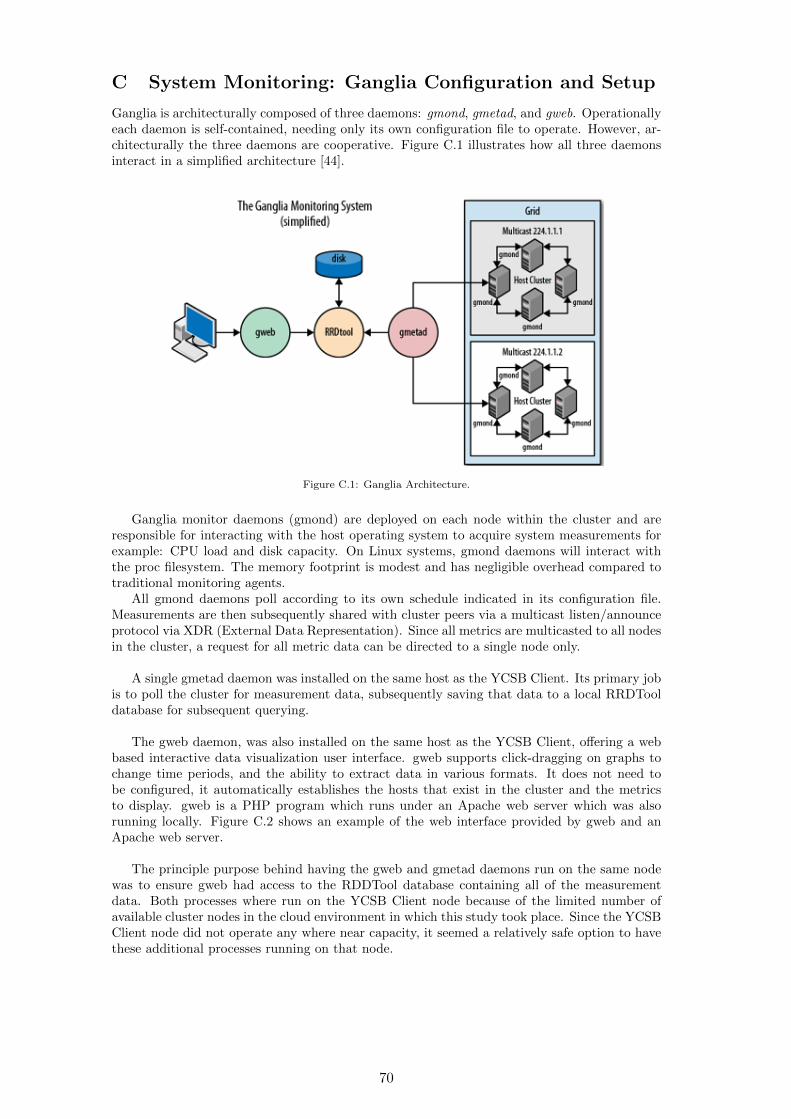
C System Monitoring: Ganglia Configuration and Setup

Ganglia is architecturally composed of three daemons: gmond, gmetad, and gweb. Operationallyeach daemon is self-contained, needing only its own configuration file to operate. However, ar-chitecturally the three daemons are cooperative. Figure C.1 illustrates how all three daemonsinteract in a simplified architecture [44].

Figure C.1: Ganglia Architecture.

Ganglia monitor daemons (gmond) are deployed on each node within the cluster and areresponsible for interacting with the host operating system to acquire system measurements forexample: CPU load and disk capacity. On Linux systems, gmond daemons will interact withthe proc filesystem. The memory footprint is modest and has negligible overhead compared totraditional monitoring agents.

All gmond daemons poll according to its own schedule indicated in its configuration file.Measurements are then subsequently shared with cluster peers via a multicast listen/announceprotocol via XDR (External Data Representation). Since all metrics are multicasted to all nodesin the cluster, a request for all metric data can be directed to a single node only.

A single gmetad daemon was installed on the same host as the YCSB Client. Its primary jobis to poll the cluster for measurement data, subsequently saving that data to a local RRDTooldatabase for subsequent querying.

The gweb daemon, was also installed on the same host as the YCSB Client, offering a webbased interactive data visualization user interface. gweb supports click-dragging on graphs tochange time periods, and the ability to extract data in various formats. It does not need tobe configured, it automatically establishes the hosts that exist in the cluster and the metricsto display. gweb is a PHP program which runs under an Apache web server which was alsorunning locally. Figure C.2 shows an example of the web interface provided by gweb and anApache web server.

The principle purpose behind having the gweb and gmetad daemons run on the same nodewas to ensure gweb had access to the RDDTool database containing all of the measurementdata. Both processes where run on the YCSB Client node because of the limited number ofavailable cluster nodes in the cloud environment in which this study took place. Since the YCSBClient node did not operate any where near capacity, it seemed a relatively safe option to havethese additional processes running on that node.

70

Figure C.2: Example Ganglia Web Interface.

71

Documents

Benchmarking Replication in NoSQL Data Stores · Benchmarking Replication in NoSQL Data Stores by Gerard Haughian ... As such this study paves the way for a new replication benchmarking