Benchmarking Quantum Annealing Controls with Portfolio Optimization

Erica Grant∗ and Travis S. Humble†

Quantum Computing Institute,Oak Ridge National Laboratory

Oak Ridge, TN, 37830

Benjamin Stump‡

National Transportation Research CenterOak Ridge National Laboratory

Knoxville, TN, 37932

Quantum annealing offers a novel approach to finding the optimal solutions for a variety ofcomputational problems, where the quantum annealing controls influence the observed performanceand error mechanisms by tuning the underlying quantum dynamics. However, the influence of theavailable controls is often poorly understood, and methods for evaluating the effects of these controlsare necessary to tune quantum computational performance. Here we use portfolio optimizationas a case study by which to benchmark quantum annealing controls and their relative effects oncomputational accuracy. We compare empirical results from the D-Wave 2000Q quantum annealerto the computational ground truth for a variety of portfolio optimization instances. We evaluateboth forward and reverse annealing methods and we identify control variations that yield optimalperformance in terms of probability of success and probability of chain breaks.

I. INTRODUCTION

Optimization is integral to many scientific and indus-trial applications of applied mathematics including ver-ification and validation, operations research, data ana-lytics, and logistics, among others [1, 2]. In many cases,exact methods of solution, including stochastic optimiza-tion and quadratic programming, are computationally in-tractable and novel heuristics are used frequently to solveproblems in practice [3]. Quantum annealing (QA) of-fers a novel meta-heuristic that uses quantum mechanicsfor unconstrained optimization by encoding the problemcost function in a Hamiltonian [4, 5]. Recovery of theHamiltonian ground state solves the original optimiza-tion problem and this approach has been mapped to avariety of application areas [6–9]. Several experimentalefforts have realized quantum annealers [10–12], and ap-plication benchmarking of these systems has shown QAis capable of finding the correct result with varying prob-ability of success [13–19].

QA performance depends implicitly on the complexityof the underlying problem instance as well as the controlsthat implement the heuristic [20, 21]. Presently, thereare multiple controls available to program quantum an-nealers that may each impact the observed probabilityof success. Notionally, the controls may be categorizedas pre-processing, annealing, and post-processing meth-ods. Whereas pre-processing controls define the encoded

∗ Also at Bredesen Center,University of TennesseeKnoxville, TN, 37996; egrant8@vols.utk.edu† Also at Bredesen Center,University of TennesseeKnoxville, TN, 37996; humblets@ornl.gov‡ stumpbc@ornl.gov

Hamiltonian and embedding onto the quantum annealer[22, 23], the annealing controls drive the time-dependentphysics of the device and the underlying quantum state[20, 24] while post-processing controls influence the read-out and decoding of the observed results [25, 26]. Col-lectively, the choice for each type of control may eitherenhance or impede the probability of reaching the en-coded ground state and, therefore, impact the resultingsolution state.

Here we benchmark a selection of pre-processing andannealing controls available in a programmable quan-tum annealer [10] using a well-defined class of uncon-strained optimization problems derived from the appli-cation of Markowitz portfolio theory [27]. As a variantof binary optimization, Markowitz portfolio optimizationselects the subset of investment assets expected to yieldthe highest return value and minimal risk while stay-ing within a total budget constraint [27, 28]. We castthis problem which forms a complete graph as uncon-strained optimization and benchmark the probability ofsuccess for QA to recover the global optimum. In par-ticular, we benchmark the pre-processing and annealingcontrols available in the 2000Q, a programmable quan-tum annealer from D-Wave Systems [10]. This includescontrols for mapping the logical problem onto hardwareand scheduling the annealing process. We gather insightinto the underlying dynamics using multiple measures ofsuccess tested across an ensemble of randomly generatedinstances of portfolio optimization.

Previous research has benchmarked QA in compari-son to classical heuristics for solving various optimizationproblems [14, 29, 30]. In particular, several variationsof portfolio optimization have been used to benchmarkQA performance [20, 31, 32]. Rosenberg et al. demon-strated several encodings of a multi-period Markowitzportfolio optimization formulation to be solvable using a

arX

iv:2

007.

0300

5v1

[qu

ant-

ph]

6 J

ul 2

020

2

quantum annealer and found promising initial results inprobability to find the optimal result [32]. Venturelli etal. benchmarked a similar mean-variance model of portfo-lio optimization using a hybrid solver that couples quan-tum annealing with a genetic algorithm [20]. This hybridalgorithm was found to be 100x faster than forward an-nealing alone. In this work, we present a formulation ofportfolio optimization to benchmark the behaviour of QAcontrols. We present studies focused on the variability insuccess with respect to available quantum annealing con-trols in an attempt to establish a methodology for findingan optimal set of controls which yield the highest solutionquality [33, 34].

The presentation is organized as follows. In Sec. II, wereview quantum annealing and the the available controls.In Sec. III, we provide an overview of the benchmarkingmethods and the use of Markowitz portfolio selection forproblem specification. In Sec. IV, we present the resultsfrom experimental testing using different quantum an-nealing controls with the 2000Q. We offer conclusions inSec. V.

II. QUANTUM ANNEALING

Under ideal conditions, forward annealing evolvesa quantum state |Ψ(t)〉 under the time-dependentSchrodinger equation

i~∂

∂t|Ψ(t)〉 = H(t)|Ψ(t)〉 t ∈ [0, T ] (1)

where T is the total forward annealing time and the time-dependent Hamiltonian is

H(t) = A(s(t))H0 +B(s(t))H1. (2)

where s(t) ∈ [0, 1] is the control schedule and time-dependent amplitudes A(s) and B(s) satisfy the condi-tions A(0) � B(0) and A(1) � B(1). We consider theinitial Hamiltonian H0 = −

∑ni σ

xi as a sum of Pauli-

X operators σxi over n spins. The final Hamiltonian H1

represents the unconstrained optimization problem witha corresponding ground state that encodes the compu-tational solution. We will consider below only problemsrepresented using the Ising Hamiltonian

H1 =∑i

hiσzi +

∑i,j

Ji,jσzi σ

zj + β (3)

where hi is the bias on the ith spin, Ji,j is the couplingstrength between the ith and jth spin, σz

i is the Pauli-Z operator for the ith spin, and β is a problem-specificconstant. The Ising Hamiltonian is well known for repre-senting a variety of unconstrained optimization problems[35].

Instantaneous eigenstates at time t are defined as

H(t)|Φj(t)〉 = Ej(t)|Φj(t)〉 (4)

where j ranges from 0 to N − 1 with N = 2n the di-mension of the Hilbert space. For an initial quantumstate prepared in the lowest-energy eigenstate at timet = 0, i.e, |Ψ(0)〉 = |Φ0(0)〉, adiabatic evolution underthe Hamiltonian in Eq. (2) to time T will prepare thefinal state |Ψ(T )〉 = |Φ0(T )〉 with high probability pro-vided T is sufficiently large. In particular, the evolutionmust be much longer than the inverse square of the min-imum energy gap between the ground and first excitedstates [4]. At time T , the prepared quantum state is mea-sured in the computational basis to generate a candidatesolution for the encoded problem.

Another variation of quantum annealing reverses thetime-evolution process by beginning in an eigenstate ofH1. Known as reverse annealing, the initial quantumstate evolves under Eq. (2) in the reverse direction. TheHamiltonian starts as H1 at time t = 0 and evolves back-ward to a point sp in the control schedule that corre-sponds to time t1. The Hamiltonian then pauses for atime tp = t2− t1 before evolving in the forward directionfrom the value sp at time t2 back to the final Hamil-tonian at time T ′, where the latter time represent thereverse annealing time. The control schedule for reverseannealing is then defined as [36, 37]

s′(t) =

1 +

(sp−1)t1

t, 0 ≤ t ≤ t1sp, t1 ≤ t ≤ t2sp +

(1−sp)(T ′−t2) (t− t2) t2 ≤ t ≤ T ′

(5)

The differences in the control schedules of forwardand reverse annealing are demonstrated in Fig. 1, wherea linear reverse annealing schedule is compared to alinear forward annealing schedule using the amplitudesA(s) = (1 − s) and B(s) = s. Notably, forward anneal-ing controls increase monotonically with time whereasreverse annealing controls include a change in the direc-tion of the control schedule where the ramp time froms = 1 to sp is tr = t1, the time paused at sp is tp, andthe quench time back from sp to s = 1 is tq = T ′ − t2.

A. Quantum Annealing Controls

In practice, there are non-ideal behaviours that arise inpractical implementations of quantum annealing. Equa-tions (1)-(5) represent quantum annealing under idealadiabatic conditions that are difficult to realize in ac-tual quantum devices. Real-world quantum annealershave limits in the ability to control the Hamiltonian andquantum dynamics [38]. In addition, the presence of ill-characterized environmental couplings give rise to fluxnoise [39]. The imperfect setting of the Hamiltonian pa-rameters (h, Ji,j) by the analog control circuits gives riseto a small intrinsic control error [34]. These errors un-dermine the accuracy of the physical hardware [22, 38].Finally, annealing too quickly may violate the essentialadiabatic condition [4], while annealing too slowly maylead to undesired thermal excitations of the quantum

3

FIG. 1. The control schedule for reverse annealing (RA)compared to forward annealing (FA) plotted with respect totime. The control schedule for forward annealing starts att = 0, s = 0 and anneals at a constant rate to t = T, s = 1,while the control schedule for reverse annealing starts at t = 0with s = 1, decreases to a value sp at time t1, pauses for timetp = t2 − t1, and then increases to s = 1 at time T ′.

state due non-zero temperature fluctuations [40]. Thismultitude of effects complicates both the description ofquantum annealing as well as the assessment of its per-formance.

Given the implicit dependence on several competingfactors, a variety of strategies have emerged for control-ling quantum annealing to maximize probability of suc-cess in recovering the ground state and minimizing errorsin the quantum computational solution. These controlstrategies include efficiently mapping the problem Hamil-tonian onto the physical hardware Hamiltonian, tuningannealing schedule, applying variable transformations tomitigate control biases, and using reverse annealing torefine initial solutions [34, 36].

We investigate a subset of controls available in the D-Wave 2000Q, a programmable quantum annealer com-posed from an array of superconducting flux qubits oper-ated at cryogenic temperatures [41]. The 2000Q consistsof up to 2048 physical qubits arranged in a sparsely con-nected array whose governing Hamiltonian is describedby a time-dependent, transverse Ising Hamiltonian [42]for which with the Hamiltonian parameters in the de-vice can be programmed individually. This enables abroad variety of computational problems, including port-folio optimization, to be realized. We briefly review someof the controls available to influence the success of solvingthese problems using quantum annealing.

1. Problem Embedding

The Hamiltonian encoding the computational prob-lem must be mapped into the physical hardware while

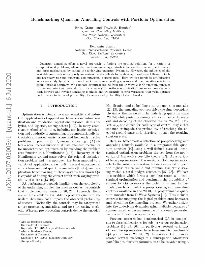
satisfying the constraints of limited connectivity. The2000Q hardware supports a sparse Chimera graph inwhich physical qubits are not fully connected but haveaverage degree 6. A fully connected graph, like in Fig. 2,must be mapped onto the more sparse Chimera graph.A single spin from the input Hamiltonian may be re-alized in hardware using multiple physical qubits thatform a strongly interacting representative chain of spins.By judiciously choosing these chains and their interac-tions, the original input Hamiltonian may be constructed.This process, known as embedding, depends on the inputproblem as well as the target hardware connectivity. Ingeneral, embedding is NP-hard for arbitrary input graphs[43], and there are upper limits on the maximum graphthat can be embedded [44]. For example, the largest fullyconnected problem that can be embedded onto the 2000Qhas ∼ 60 spins, while the limit in practice depends on thenumber of faulty/inactive physical qubits in the device.

Embedding algorithms that optimize chain length maygreatly reduce the number of physical qubits required byconsidering problem symmetry as well as the location offaults in the hardware. We highlight two embedding algo-rithms widely used in programming the 2000Q. The firstmethod by Cai, Macready, and Roy is based on random-ized placement and search for the weighted shortest pathbetween spin chains [45]. This method, which we denoteas CMR, applies to arbitrary input graphs but typicallycreates a distribution of chain lengths. By contrast, asecond method by Boothby, King, and Roy based on aclique embedding typically generates shorter and uniformchain lengths of size

lc =n

4+ 1 (6)

for n logical spins [46]. A representative example of theoutput from these different methods is shown in Fig. 2using a fully connected problem with 20 logical spins.Both methods are available in the D-Wave Ocean soft-ware library [47].

Ensuring an embedded chain of qubits collectively rep-resents a single logical variable requires an intra-chaincoupling that is larger in magnitude than the the inter-chain couplings between chains. In other words, the chainof physical qubits must be strongly coupled to remain asingle logical spin. However, it is possible for chains tobecome “broken” in so far as individual physical spinswithin the chain differ in their final state. In general,chain breaks arise from non-adiabatic dynamics that leadto local excitation out of the lowest energy state withlonger chains more susceptible to these effects [34, 48].

An additional control is required for decoding embed-ded chains to recover the computed logical spin state. Inthe absence of chain breaks, the logical value is inferreddirectly from the unanimous selection of a single spinstate by every physical qubit. In the presence of chainbreaks, several strategies may be employed to decide thelogical value including majority vote [34], which selectsthe logical spin value as the value that occurs with thehighest frequency in a chain.

4

FIG. 2. The embedding of a 20 logical spin complete graphonto a Chimera graph structure. Figure a) is complete K20

graph which is fully connected with 20 nodes and 190 edgeswhere each node represents a logical spin and each edge isa coupling between spins. Figure b) is the CMR algorithmwhich requires the allocation of 23 unit cells and c) is theclique embedding algorithm which requires the allocation of15 unit cells. The nodes represent physical qubits, lines arethe couplings between physical qubits, and each color is adifferent physical spin chain corresponding to a logic spin.

2. Spin Reversal

Interactions between embedded chains arise from therequired coupling between the logical spins. However,imperfections in the control of these spins lead to smallbiases that can become non-negligible for larger qubitchains and contribute to the complex dynamics describ-ing the device. In turn, the probability for finding theexpected ground state solution can decrease do to thesebias errors. The influence of these errors on the compu-

tational result may be mitigated by using spin reversaltransforms to average out biases.

As a gauge transformation, spin reversal redefines theHamiltonian by replacing the biases and couplings for asubset of spins with their negated value [33, 34]. Thistransformation maintains the ground state of the logicalproblem. However, this transformation flips the sign ofrandomly selected qubits so that on average their biasis reduced. This strategy mitigates errors on individualspins by balancing the noise on the device prior to an-nealing [26]. The number of selected spins as well as theparameter g that defines the number of times to performthe transformation.

3. Annealing Schedules

Tailoring the annealing amplitudes A(s) and B(s) isperhaps the most direct method to control forward an-nealing. The annealing schedules control the rate ofchange of the H(t), which must be sufficiently slow toapproximate the adiabatic condition [49]. An exam-ple of the amplitudes in a D-Wave 2000Q is shown inFig. 3. While forward annealing on the D-Wave 2000Q,A(s(t)) >> B(s(t)) at t = 0, A(s(t)) decreases andB(s(t)) increases for 0 < t < T , and B(s(t)) >> A(s(t))at t = T .

FIG. 3. The amplitudes of the D-Wave 2000Q over the rangeof control schedule as measured from s = 0 to s = 1 in incre-ments of 0.001.

The optimal annealing time is problem dependent andinversely proportional to the minimum energy gap [4],and, in general, the value and position of the minimumenergy gap for a given H(t) is typically unknown andhard to identify. Extending the annealing time T arbi-trarily long may not only be limited by hardware pa-rameters but also be counter-productive due to compet-ing thermal processes that depopulate the ground state[25, 50]. There is an upper limit to the total job time(NsT ≤ 1 s) as well as total annealing time (T ≤ 2 s) onthe D-Wave 2000Q.

5

When reverse annealing, the three primary parametersfor control are the initial state ei, the pause point sp, andthe pause duration tp. The times tr and tq can also bemanipulated, but we keep these constant and symmetricfor our experiments. Reverse annealing uses ei to set theinitial quantum state, which may be based on the outputof forward annealing, a heuristically computed candidate,a random state or other methods. Our experiments use apre-computed initial state, e.g., using forward annealing.An iterative procedure is then used which replaces theei of each subsequent reverse annealing sample with theoutput from previous reverse annealing iteration.

B. Quantum Annealing Metrics

We characterize quantum annealing using the proba-bility of success

ps = |〈Φ0(T )|ρ|Φ0(T )〉|2 (7)

defined as the overlap of the final, potentially mixedquantum state ρ prepared by QA with the pure-statedescribing the expected computational outcome Φ0(T ).Empirically, the probability of success is estimated fromthe frequency with which the observed solution statematches the expected outcome. When the expectedground state solution is known, we define the statisticδi = 1 if the i-th sample matches the known ground stateand δi = 0 if it does not. For the k-th problem Hamil-tonian instance, the estimated probability of success isthen defined as

p(k)s =1

Ns

Ns∑i=1

δi (8)

where Ns is the total number of samples. The averageover an ensemble of Np problem instances is defined as

ps =1

Np

Np∑k

p(k)s . (9)

A second metric for characterizing quantum annealingperformance, and especially the non-adiabatic dynamics,is the number of chain breaks observed in the recoveredsolution samples. As noted above, a chain break is ob-served when the chain of physical qubits embedding alogical spin has more than one unique spin value. Weestimate the probability of chain breaks for a probleminstance

p(k)b =

1

Ns

Ns∑i=1

εi (10)

where the statistic εi = 1 when the i-th sample solutioncontains at least one broken chain for any of the logicalspins and εi = 0 when no embedded chain is broken. The

average probability of chain breaks over an ensemble ofNp problem instances is then defined as

pb =1

Np

Np∑k

p(k)b . (11)

It is important to note that the effects of chain breakscan be mitigated by post-processing methods, such asmajority vote, which make hard decisions on the logicalspin value.

While the above metrics quantify the probability withwhich quantum annealing recovers the correct solution,additional information about computational performancecomes from the distribution of all solution samples ob-tained. In particular, the distribution over sample ener-gies provides a representation for the weight of errors inthe solution samples. A distribution concentrated aroundthe lowest energy indicates a small number of errors inthe computed solutions, while a broad or shifted distri-bution hints at a larger number of errors. We denotethe energy computed from the i-th solution sample asE(i) and we define the j-th energy bin as hj . The bin hjcounts the number of samples with an energy in the range[j, j+1]∆ where ∆ controls the granularity of binning theenergies. The resulting set {(j∆, hj)} approximates theenergy distribution of the sampled solutions.

III. BENCHMARKING METHODS

We benchmark performance of the quantum anneal-ing controls presented in Sec. II using a variant of con-strained optimization derived from Markowitz portfoliotheory. We recast this problem as unconstrained op-timization before reducing to quadratic unconstrainedbinary optimization (QUBO) form. The latter form iseasily translated to the classical Ising spin Hamiltonianand, subsequently, to the problem Hamiltonian definedby Eq. (3).

A. Markowitz Portfolio Selection

Portfolio optimization selects the best allocation of as-sets to maximize expected returns while staying withinthe budget and minimizing financial risk. The Markowitztheory for portfolio selection focuses on diversificationof the portfolio for risk mitigation [27]. Instead of allo-cating high percentages of a budget toward assets withthe highest projected returns, the budget is distributedover assets that minimize correlation between the asset’shistorical prices. In this model, the covariance betweenpurchasing prices serves as a proxy for risk in which pos-itively correlated assets are considered to be more risky.We review the methods by which the benchmark prob-lems are generated and solved in this section.

We consider Markowitz portfolio optimization as aquadratic programming problem that determines the

6

fraction of available budget b to allocate toward pur-chasing assets with the goal of maximizing returns whileminimizing risk. By selecting a partition number w, thefraction pw = 1

2(w−1) represents the granularity of the par-tition. The portfolio optimization problem selects howmany of those partitions to allocate toward each assetwith an integer zu. Thus, the fraction of b to invest ineach uth asset is given by pwbzu, and portfolio optimiza-tion identifies how much of the m assets to select giventhe budget b and a risk threshold c. Thus, portfolio se-lection is cast as

maxz

m∑u=1

ruzu

s.t.

m∑u=1

pwbzu = b,

m∑u,v=1

cu,vzuzv ≤ c

(12)

where for the uth asset ru is the expected return and cu,vis the historical price correlation between assets u, v.

In Eq. (12), the first term represents maximization ofthe expected returns over the available assets. Thereare many methods for forecasting expected returns, e.g.,based on market price, expert judgement, and historicalprice data [51, 52]. For simplicity, we model expectedreturns as

ru = pwau (13)

where au is the average of au, the history of price datafor the uth asset. The first constraint in Eq. (12) placesa hard constraint on the total allocation of assets to sumto b. We emphasize that this constraint penalizes port-folios that do not allocate the entire budget as well asthose that over commit. Finally, the second constraintaccounts for diversification by asserting that the sum ofcovariance between asset prices cu,v be less than or equalto the risk threshold c. The historical price covariance iscalculated as the correlation between pairs of assets bycomparing the pw fraction of each asset’s historical pricedata. Here covariance is defined as

cu,v =p2w∑Nf

l=1(au,l − au)(av,l − av)

Nf − 1(14)

where au,l is the lth historical price value for asset u andNf is the number of price points in the historical data.

We solve this variation of Markowitz portfolio selectionusing quantum annealing by casting the formulation inEq. (12) into quadratic unconstrained binary optimiza-tion (QUBO). We express the integer variable zu as aw-bit binary expansion

zu =

w∑k=1

2k−1xi(u,k) (15)

with xi ∈ {0, 1} and the composite index i(u, k) = (u −1)w + k. The expected returns are then expressed as

ruzu =

w∑k=1

2k−1ruxi(u,k) (16)

while the allocation constraint becomes the penalty term

−( m∑u=1

w∑k=1

2k−1pwbxi(u,k) − b)2

(17)

We consider a correlation threshold c = 0 such that thecorrelation constraint becomes

m∑u,v

cu,vzuzv =

m∑u,v

w∑k,k′

2k−12k′−1cu,vxi(u,k)xj(v,k′). (18)

Our formulation of Markowitz portfolio selection as anunconstrained optimization problem then becomes

maxx

θ1

n∑i

rixi

− θ2(

n∑i

2k−1bpwxi − b)2

− θ3n∑i,j

ci,jxixj

(19)

where the problem size n = mw, ri = 2k−1ru, ci,j =

2k−12k′−1cu,v, and θ1, θ2 and θ3 are Lagrange multipliers

used to weight each term for maximization or penaliza-tion.

For purposes of benchmarking, we generate an ensem-ble of problem instances by sampling from uniform ran-dom price data with a seed of b/5 . A random numberis drawn as the initial price au,1 and every subsequenthistorical price point up to the purchasing price is −25%to +25% of the previous price au,l. The price range wasset to be between b/10 and b with Nf = 100 historicalprice points per asset. In addition, we normalize all au,lby au,Nf

to keep all asset prices to a similar range.We set θ1 = 0.3, θ2 = 0.5, θ3 = 0.2 in the problem in-

stances where θ2 is set higher to enforce the budget con-straint. These weights were chosen after testing whichcombination stayed on budget and gave some diversity.By keeping θ2 constant and increasing θ3 while decreas-ing θ1, an investor could increase the diversity relativeto the potential returns and vice versa when decreasingθ3 relative to θ1. We generate 1000 problems for eachproblem size with m = 2, 3, 4, 5 assets and w = 4 slices.

B. QUBO to Ising Hamiltonian

We formalize the unconstrained portfolio optimizationproblem in Eq. (19) to quadratic unconstrained binary

7

optimization (QUBO) as

minx

( n∑i

qixi +

n∑i,j

Qi,jxixj + γ)

(20)

where qi is the linear weight for the ith spin, Qi,j is thequadratic weight for interactions between the ith and jth

bits, and γ is a constant. Note that our definition ofQUBO expresses optimization as minimization by switch-ing the sign of Eq. (19) to be consistent with the use ofquantum annealing to recover the lowest-energy state.The corresponding relationships with the original prob-lem instance are given as

qi = −θ1ri − 2θ2b2pw

Qi,j = θ2b2p2w + θ3ci,j

γ = θ2b2

(21)

Similarly, the quadratic binary form may be reduced toa classical Ising Hamiltonian

H(s) =∑i

sihi +∑i,j

sisjJij + β (22)

where spin si ∈ {−1, 1} is defined by si = 2x1 − 1 withs = (s1, s2, . . . , sn) while hi is the spin weight, Jij is thecoupling strength, and β is a problem-specific constant.The parameters for the Ising Hamiltonian are given as

Ji,j =1

4Qi,j

hi =qi2

+∑j

Ji,j

β =1

4

∑i,j

Qi,j +1

2

∑i

qi + γ

(23)

The classical Ising formulation is then converted intoa corresponding quantum Ising Hamiltonian given byEq. (3) using the correspondence si → σz

i .

C. Computational Methods

We used a D-Wave 2000Q quantum annealer for ourexperiments. We calculate the probability of success,the probability of chain breaks, and the energy distri-bution across each problem instance. For each instance,we estimated these metrics by collecting Ns = 1000 sam-ples of the computed solution. We used D-Wave’s solverAPI (SAPI) with Python 2.7 to solve each instance ofMarkowitz portfolio selection using the hardware controlsoutlined in Sec. II A. We ran 1, 000 samples per problemover a set of 1, 000 problems for forward annealing exam-ples an 100 problems for revere annealing examples. Weimplement the majority vote post-processing techniquefor any broken chains to interpret raw solutions returnedby the 2000Q. The program implementation and data

sets collected from these experiments are available online[53].

For benchmarking purposes, we also solved each prob-lem instance using brute force search for the minimalenergy solutions of the QUBO formulation. We com-puted the complete energy spectrum for each portfolioinstance. These energy spectrum and the correspondingstates were then used as ground truth for testing the ac-curacy of results obtained from quantum annealing. Bysorting the spectrum, we benchmarked the success of re-verse annealing using initial states ei sampled from thesedifferent parts of the spectrum.

IV. RESULTS

We benchmark quantum annealing controls by evaluat-ing their influence on the probability of success and prob-ability of chain breaks across problem instances. We firstcharacterize how problem parameters influence the base-line performance by estimating the probability of successfor forward annealing using T = 15 µs, g = 0, and arandomized embedding strategy. As shown in Fig. 4, wecompare ps for two cases of w = 1 and w = 4 acrossincreasing n. The estimated probability of success forproblems with w = 4 is consistently higher for problemswith no slicing.

FIG. 4. The average probability of success over 1000 problemseach with 1000 samples using CMR, g = 0, and T = 15 µ s.The comparison is between a set of problems from problemsizes 8 to 20 for w = 1 (yellow) and w = 4 (blue). The prob-lems set to slices w = 1 are much less complex and thereforehave a much higher probability of success.

These results are explained by the energy spectra forthe different problem parameters, which indicate sharpdifferences in the density of states. As shown in Fig. 5, atypical problem instance with w = 4 has a much higherdensity of states than those with no slicing (w = 1). In-tuitively, the single-slice behavior results from the spec-ification that the price for each asset is proportional tobudget, and, therefore, only a single asset may be selected

8

FIG. 5. Probability histogram (100 bins) of all possible ener-gies for problem of size 20 where a) is of w = 1 and b) is ofw = 4. There is a higher density of states close to e0 in figureb) and therefore more opportunities to jump to an excitedstate throughout the sample.

without penalty when w = 1. However, the number ofsatisfying solutions v increases for arbitrary w combina-torially and, as shown in Appendix A,

v =(2w−1 +m− 1)!

(2w−1)!(w − 2)!. (24)

Consequently, the probability to recover the lowest-energy state competes with these closely spaced, higherenergy solutions, which leads to a corresponding decreasein the probability of success. For the remaining bench-mark tests below, we chose w = 4 as it represents a morechallenging test for the quantum annealer as well as agreater interest to real-world financial applications.

A. Benchmarking Forward Annealing Controls

1. Embedding

Embedding generates and places the physical spinchains for each logical spin on the quantum annealinghardware. We evaluated the CMR and clique embed-ding algorithms described in Sec. IV A 1 by estimat-ing the probability of success across problem sizes ofm = 8, 12, 16, and 20 logical spins. For all problem in-stances of a same problem size, we use the same em-bedding because they require the same number of fullyconnected logical spins. We set the parameters of theembedded Ising Hamiltonian by scaling the inter-chaincouplings Ji,j to lie in the range [−1,+1]. We scale all

Ji,j using a rescale factor of 1jmax

where jmax is the largest

Ji,j so all embedded Ji,j = 1jmax

Ji,j . This scales all Ji,jto be between + − 1. The intra-chain coupling strengthis set to −1 to have a negative bias stronger than the Ji,jvalues which range −10−1 ≤ Ji,j ≤ 10−1 due to our datageneration and normalization techniques.

The average chain length 〈lc〉 from CMR and cliqueembedding methods grows with the number of logicalspins n. The average is computed with respect to allchains in an embedding and plotted with respect to nin Fig. 6. As expected by Eq. (6), the clique embed-ding method has a uniform chain length for each n. Bycontrast, the CMR method generates chains of variablelength as indicated by the the average chain length andvariance shown in the plot.

FIG. 6. The average chain length over all chains for a givenembedding clique and CMR embedding as n increases.

From each of the embedding methods, we estimate theprobability of success and probability of broken chains.As shown in Fig. 7, we observe very small differences inboth metrics with increasing problem size. From fittingthe resulting point to an exponential, we find ps decayssub-exponentially with respect to n with rate −0.523 forthe CMR embedding and rate −0.528 for the clique em-bedding. We find that pb grows at a sub-exponentialrate of 0.1824 for CMR embedding and 0.1656 for cliqueembedding as n increases. There is not a significant dif-ference in the ps performance between CMR and cliqueembedding, but clique embedding requires a fewer num-ber of spins as n increases and shows a slight improve-ment in pb. Therefore, we chose to use clique embeddingfor subsequent benchmarks.

2. Forward Annealing Time

According to the adiabatic theorem, forward annealingmore slowly should increase the probability of the systemremaining in the ground state and thus increase the prob-ability of success. We varied the forward annealing timeT from 1 µs to 999µs, which is the broadest range acces-sible on the D-Wave 2000Q. As shown in the upper panelof Fig. 8, we observed statistically insignificant changes

9

FIG. 7. The ps (top) and pb(bottom) on a log scale over1, 000 samples for 1, 000 problems comparing CMR to cliqueembedding for parameter settings of g = 0 and T = 100 µs.

in the probability of success as annealing time increasedat each problem size. Fitting the average probability ofsuccess with respect to problem size for the annealingtime T = 100 µs, yields a sub-exponential decay rate forps given by −0.528 and a sub-exponential growth rate forpb given by 0.1628 as n increases. We do observe a statis-tically significant difference in the estimated probabilityof chain breaks pb with respect to forward annealing timeas shown in the lower panel of Fig. 8. For T = 100 µs,we recover a growth rate of 0.1656 for the probability ofchain breaks with respect to problem size.

3. Spin Reversal

As discussed in Sec. IV A 1, embedding maps a logicalspin to many physical spins by creating strongly cou-pled chains. Coupling of these embedded spins via Ji,jin Eq. (3) can lead small biases that may be amplified byimperfections in the hardware. A spin reversal transformmitigates against bias errors by reversing the sign of aspin in the Ising Hamiltonian. This transform preservesthe logical problem but reverses the bias error on theembedded spin chain. By randomly selecting a subset ofspins to revise, we evaluate the influence of spin-reversaltransform on the probability of success. We use g trans-forms when estimating the probability of success for agiven problem instance, such that there are Ns/g sam-ples per transform. We observed nominal improvementsin Fig. 9 by using at least g = 2 with no advantage tousing g > 2. For g = 2, we observe an sub-exponentialdecay rate of −0.505 for ps and a sub-exponential growth

FIG. 8. The average ps (top) and pb(bottom) on a log scaleover 1000 samples for 1000 problems at various annealingtimes for parameter settings of g = 0 and clique embedding.

rate of 0.146 for pb as problem size increases.

FIG. 9. The ps (top) and pb (bottom) on a log scale overNs = 1000 samples for Np = 1000 problems at g = 0 → 10)for parameter setting of T = 100µs and clique embedding.

B. Benchmarking Reverse Annealing Controls

From the reverse annealing controls listed in Sec. II A 3,we designed three experiments based on the ei for the re-verse annealing heuristic that include (i) starting in theknown ground state e0, (ii) starting in the known firstexcited state e1, and (iii) starting in the lowest-energystate obtained from 1000 forward annealing samples ef .

10

We then sweep over various schedules to find the opti-mal sp with a range of [0.1, 0.9] and tp with a range of[15 → 800]µs. The tr and tqparameters were set to beconstant and symmetric at 5µs each. Thus, the totalanneal time is T ′ = tr + tp + tq where tp is the time pa-rameter that we chose to analyze. For all experiments,we ran the reverse annealing iterative heuristic with 1000samples for 100 random problems were also used in theforward annealing experiments. We estimated the prob-ability of success for reverse annealing with respect todifferent choices for ei, sp, and tp. We compared thecombined heuristic of reverse annealing with forward an-nealing to forward annealing alone with ps, pb, as wellas the frequency of finding energies in excited states toforward annealing alone [54].

By setting ei to the ground state, we tested for pa-rameters sp and tp that decrease ps when the quantumannealer is fed the correct solution. For this experiment,ps can be thought of as the probability of staying in e0

ps(e0 → e0) = pf ∗ ps (25)

pf ∗ ps =

∑Np

i αi

Np∗∑Np

i

∑Ns

j δij

Ns(26)

where pf is the probability that forward annealingfound the ground state, αi ∈ {0, 1} indicates whetherforward annealing found the ground state for the ith

problem prior to reverse annealing, and δj ∈ {0, 1} isa variable indicating whether the jth sample of the ith

problem was measured to be the ground state with re-verse annealing. By setting ei = e1, we tested whetherreverse annealing enhances the probability to populatethe ground state. For these tests, ps estimates the prob-ability of moving from an excited state to the groundstate

ps(ee → e0) = (1− pf ) ∗ ps (27)

(1− pf ) ∗ ps =

∑Np

i (1− αi)

Np∗∑Np

i

∑Ns

j δij

Ns. (28)

In addition to testing reverse annealing at ei = e0 and e1,We tested reverse annealing in combination with forwardannealing for which ps estimates the cumulative proba-bility of finding the correct solution state.

ps(R) = p(e0 → e0) + p(ee → e0) (29)

For these experiments, we found it useful to primarilyanalyze ps(R) − p(e0 → e0) = p(ee → e0) to determineif reverse annealing improved upon the ps of forward an-nealing.

The results from setting ei = e0 for each problem witha problem size of n = 20 where m = 5 and w = 4 isshown in Fig. 10. Because the computation begins in the

correct solution state, this test measures the probabil-ity by which reverse annealing introduces errors into thecorrect solution. Ideally, ps will remain near unity for allsp and tp. We observe that reverse annealing causes thesystem to leave the ground state with ps reducing to onthe order of 10−5 by annealing back to at least s = .6and increasing tp ≥ 200µs

FIG. 10. The ps (left) and pb (right) for reverse annealingwhere ei = e0 and as s = [0.1→ 0.9] and tp = [15µs→ 800µs]for n = 20 with m = 5 assets and w = 4.

The results from setting ei = e1 with a problem sizeof n = 20 where m = 5 and w = 4 for each problemis shown in Fig. 11. A maximal value of 4.8 × 10−4 forps is found with parameters s = 0.7 and tp = 800 µs.This is is a ps one order of magnitude higher than whatis observed with forward annealing. This suggests thatif ei is very close to e0, there may be some benefit tochoosing reverse annealing over forward annealing.

FIG. 11. The ps (left) and pb (right) for reverse annealingwhere ei = e1 for each problem, s = [0.1 → 0.9], and tp =[15µs→ 800µs] for problem size 20 with 5 assets and 4 slices.

When solving optimization problems for applicationsin practice, the ground state and excited state will beunknown. However, one approach is to use reverse an-nealing in addition to forward annealing by using thelowest energy state found with 1, 000 forward annealingsamples ef as ei for another 1, 000 samples of reverseannealing. The next experiment tests whether reverse

11

annealing used in combination with forward annealing in-creases ps with a problem size of n = 20 where m = 5 andw = 4 . The experimental results from setting ei = ef isshown in Fig. 12. These tests were constructed to deter-mine when combining reverse annealing with forward an-nealing can improve upon forward annealing. Therefore,we removed the 6 problems forward annealing providedan ei = e0 and thus ps for this experiment is given byps(R)− p(e0 → e0) in this analysis. Similar to the previ-ous experiment in Fig. 11, the ps is at best on the order of10−4 at parameters s = 0.7 and tp = 400µs which is oneorder of magnitude greater than the forward annealingexperiments.

FIG. 12. The ps (left) and pb (right) for reverse annealingwhere ei = ef for each problem, s = [0.1 → 0.9], and tp =[15µs→ 800µs] for problem size 20 with 5 assets and 4 slices.The 6 problems where ef = eg were excluded. Thus, ps =p(ee → e0).

Fig. 12 shows a potential for reverse annealing to im-prove upon results found with forward annealing in ps.Therefore, we take a set of 100 problems solved with re-verse annealing and forward annealing and compare theps of forward annealing (orange) alone to the ps of reverseannealing alone (blue) to the ps with a selection of eitherforward annealing or reverse annealing (green). If fora problem forward annealing found at least one groundstate the forward annealing ps was plotted for that prob-lem (6 problems) and otherwise the reverse annealing pswas plotted (94 problems). The ps is measured over nranging from [8, 20]. The reverse annealing parametersare set to have an ei = ef , s = .7, and tp = 400µs.As shown in Fig. 13, we observe that when taking thecombination of best results from forward annealing andreverse annealing with ei = ef , we get a ps that improvesby an order of magnitude over forward annealing alonefor n = [16, 20] with a sub-exponential decay at a rate of−0.309. Note that although the blue reverse annealingtrend looks to perform the best, however this trend is ar-tificially inflated because 6 of the problems have ei = e0which has been demonstrated in Fig. 10 to yield a pson the order of 10−2 at s = .7 and tp = 400µs. Wenext visualize a histogram, as seen in Fig. 14, of all ener-gies recorded from 1000 samples returned for a set of 94

FIG. 13. The ps as a function of n over a set of 100 prob-lems each with 1000 samples. We compare reverse annealing(blue) with ei = ef , s = .7, and tp = 400µs to forward an-nealing (orange) with clique embedding, g = 0, and annealingtime = 100 µs. We also compare the combination of forwardannealing and reverse annealing where the ps is chosen byproblem (green). In this green trend, the ps is calculated us-

ing the forward annealing p(k)s for the 6 problems where for-

ward annealing would have provided reverse annealing with

an ei = e0 and the reverse annealing p(k)s for the 94 problems

where ei 6= e0.

problems where forward annealing did not find e0 withn = 20. We compare forward annealing to reverse anneal-ing where ei = ef . We observe even for problems whereneither reverse annealing or forward annealing found e0,reverse annealing still on average finds a lower energysolution than forward annealing.

FIG. 14. A probability histogram (20 bins) comparing allenergies found with forward annealing and reverse annealingfrom all 1000 samples for the 94 problems where ei 6= e0 forproblems with m = 5 assets and w = 4 .

V. CONCLUSIONS

We have benchmarked quantum annealing usingMarkowitz portfolio selection to evaluate the effects ofvarious controls on probability of success and chain

12

breaks. We have explored a variety of quantum an-nealing controls including the embedding algorithm, theforward annealing time T , and the number spin rever-sal transforms g. When comparing clique embeddingagainst CMR embedding, we found little difference inthe estimated probability of success ps as both techniquesyielded a sub-exponential decay for ps with exponents of−0.528 and −0.523, respectively. We did observe thatCMR demonstrated a slightly higher probability of chainbreaks pb, and we considered this a sufficient justificationto use the clique embedding for studying the fully con-nected problems Markowitz portfolio selection problem.

When varying the forward annealing time T ∈[1µs, 999µs], we found that pb was slightly higher in therange T = [1µs, 5µs] while increasing the annealing timefurther yielded little to no improvement. For this reason,we chose to continue all future forward annealing experi-ments using T = 100µs where the exponential decay ratein ps was −0.528. When varying g = [0, 10], we foundsmall improvements in ps between g = 0 and g = 2 wherethe exponential decay rate became −0.505 without muchchange from increasing the value of g further, and therewas no consistent difference in pb.

We benchmarked reverse annealing controls with re-spect to the parameters ei, s, and tp. We began by ob-serving the results in ps and pb at n = 20. We consis-tently observed that pb was the same order of magnitudeas with the forward annealing experiments and pb wasconsistently highest for s = 0.8. By setting ei = e0, weobserved that the ps decreases exponential as s increased.By setting ei = e1, we observed that reverse annealinghad a ps an order of magnitude higher than forward an-nealing. From these results, we conclude that when eiis close to the ground state, reverse annealing providedsome advantage over forward annealing. Because in gen-eral the ground state won’t be known for a problem, wedeveloped a heuristic which sets ei = ef where we againobserved ps to be an order of magnitude higher than us-ing forward annealing alone.

We further evaluated ps as a function of n to comparereverse annealing with ei = ef , s = 0.7, and tp = 400µsto forward annealing with clique embedding, T = 100µs,

and g = 0 alone. In particular, we used the p(k)s of

forward annealing for the 6 problem instances in which

ei = e0 and the p(k)s of reverse annealing for the 94 prob-

lems where ei 6= e0. We continued to observe reverseannealing demonstrate an order of magnitude increase inps over forward annealing alone. Lastly, by creating a his-togram which plots the lowest energies found across 1000samples for the 94 problems where ei 6= e0, we found thatreverse annealing(ei = ef ) on average finds lower energysolutions as compared to forward annealing.

In summary, the benchmarks presented here evaluate avariety of quantum annealing controls with respect to thebaseline ground truth for portfolio selection. By compar-ing the observed influence of these controls on the perfor-mance of solution accuracy, we have developed insightsinto the best selections of controls for solving these prob-lems with the highest accuracy which may help guide thefuture use of quantum annealing as a meta-heuristics foroptimization.

ACKNOWLEDGEMENTS

This work is supported by the Department of En-ergy, Office of Science, Early Career Research Program.This research used quantum computing resources of theOak Ridge Leadership Computing Facility, which is aDOE Office of Science User Facility supported underContract DE-AC05-00OR22725. This manuscript hasbeen authored by UT-Battelle, LLC under ContractNo. DE-AC05-00OR22725 with the U.S. Departmentof Energy. The United States Government retains andthe publisher, by accepting the article for publication,acknowledges that the United States Government re-tains a non-exclusive, paid-up, irrevocable, world-widelicense to publish or reproduce the published form of thismanuscript, or allow others to do so, for United StatesGovernment purposes. The Department of Energy willprovide public access to these results of federally spon-sored research in accordance with the DOE Public AccessPlan. (http://energy.gov/downloads/doe-public-access-plan).

[1] Panos M Pardalos and Judah Ben Rosen. Constrainedglobal optimization: algorithms and applications, volume268. Springer, 1987.

[2] Jung-Fa Tsai, John Gunnar Carlsson, Dongdong Ge,Yi-Chung Hu, and Jianming Shi. Optimization theory,methods, and applications in engineering 2013. Mathe-matical Problems in Engineering, 2014, 2014.

[3] Mark W Krentel. The complexity of optimization prob-lems. In Proceedings of the eighteenth annual ACM sym-posium on Theory of computing, pages 69–76, 1986.

[4] Edward Farhi, Jeffrey Goldstone, Sam Gutmann, andMichael Sipser. Quantum computation by adiabatic evo-

lution. arXiv preprint quant-ph/0001106, 2000.[5] Satoshi Morita and Hidetoshi Nishimori. Mathematical

foundation of quantum annealing. Journal of Mathemat-ical Physics, 49(12):125210, 2008.

[6] Hristo N Djidjev, Guillaume Chapuis, Georg Hahn,and Guillaume Rizk. Efficient combinatorial opti-mization using quantum annealing. arXiv preprintarXiv:1801.08653, 2018.

[7] Florian Neukart, Gabriele Compostella, Christian Seidel,David Von Dollen, Sheir Yarkoni, and Bob Parney. Traf-fic flow optimization using a quantum annealer. Frontiersin ICT, 4:29, 2017.

13

[8] Tobias Stollenwerk, Bryan OGorman, Davide Venturelli,Salvatore Mandra, Olga Rodionova, Hokkwan Ng, Ba-navar Sridhar, Eleanor Gilbert Rieffel, and RupakBiswas. Quantum annealing applied to de-conflicting op-timal trajectories for air traffic management. IEEE trans-actions on intelligent transportation systems, 21(1):285–297, 2019.

[9] Roman Martonak, Giuseppe E Santoro, and Erio Tosatti.Quantum annealing of the traveling-salesman problem.Physical Review E, 70(5):057701, 2004.

[10] Mark W Johnson, Mohammad HS Amin, SuzanneGildert, Trevor Lanting, Firas Hamze, Neil Dickson,Richard Harris, Andrew J Berkley, Jan Johansson, PaulBunyk, et al. Quantum annealing with manufacturedspins. Nature, 473(7346):194–198, 2011.

[11] Trevor Lanting, Anthony J Przybysz, A Yu Smirnov,Federico M Spedalieri, Mohammad H Amin, Andrew JBerkley, Richard Harris, Fabio Altomare, Sergio Boixo,Paul Bunyk, et al. Entanglement in a quantum annealingprocessor. Physical Review X, 4(2):021041, 2014.

[12] S. H. W. van der Ploeg, A. Izmalkov, M. Grajcar, U. Hub-ner, S. Linzen, S. Uchaikin, Th. Wagner, A. Yu. Smirnov,A. Maasen van den Brink, M. H. S. Amin, and et al.Adiabatic quantum computation with flux qubits, firstexperimental results. IEEE Transactions on Applied Su-perconductivity, 17(2):113119, Jun 2007.

[13] Helmut G Katzgraber, Firas Hamze, and Ruben S An-drist. Glassy chimeras could be blind to quantumspeedup: Designing better benchmarks for quantum an-nealing machines. Physical Review X, 4(2):021008, 2014.

[14] James King, Sheir Yarkoni, Mayssam M Nevisi, Jeremy PHilton, and Catherine C McGeoch. Benchmarking aquantum annealing processor with the time-to-targetmetric. arXiv preprint arXiv:1508.05087, 2015.

[15] Zheng Zhu, Andrew J Ochoa, Stefan Schnabel, FirasHamze, and Helmut G Katzgraber. Best-case perfor-mance of quantum annealers on native spin-glass bench-marks: How chaos can affect success probabilities. Phys-ical Review A, 93(1):012317, 2016.

[16] Michael Jarret, Stephen P Jordan, and Brad Lackey. Adi-abatic optimization versus diffusion monte carlo meth-ods. Physical Review A, 94(4):042318, 2016.

[17] Daniel OMalley, Velimir V Vesselinov, Boian S Alexan-drov, and Ludmil B Alexandrov. Nonnegative/binarymatrix factorization with a d-wave quantum annealer.PloS one, 13(12), 2018.

[18] Tameem Albash and Daniel A Lidar. Demonstration of ascaling advantage for a quantum annealer over simulatedannealing. Physical Review X, 8(3):031016, 2018.

[19] Akshay Ajagekar, Travis Humble, and Fengqi You. Quan-tum computing based hybrid solution strategies for large-scale discrete-continuous optimization problems. Com-puters & Chemical Engineering, 132:106630, 2020.

[20] Davide Venturelli and Alexei Kondratyev. Reverse quan-tum annealing approach to portfolio optimization prob-lems. Quantum Machine Intelligence, 1(1-2):17–30, 2019.

[21] Gregory Quiroz. Robust quantum control for adiabaticquantum computation. Physical Review A, 99(6):062306,2019.

[22] Walter Vinci, Tameem Albash, Gerardo Paz-Silva, ItayHen, and Daniel A Lidar. Quantum annealing correctionwith minor embedding. Physical Review A, 92(4):042310,2015.

[23] Zhengbing Bian, Fabian Chudak, Robert Brian Israel,Brad Lackey, William G Macready, and Aidan Roy. Map-ping constrained optimization problems to quantum an-nealing with application to fault diagnosis. Frontiers inICT, 3:14, 2016.

[24] Jeffrey Marshall, Davide Venturelli, Itay Hen, andEleanor G Rieffel. Power of pausing: Advancing un-derstanding of thermalization in experimental quantumannealers. Physical Review Applied, 11(4):044083, 2019.

[25] Kristen L Pudenz, Tameem Albash, and Daniel A Li-dar. Error-corrected quantum annealing with hundredsof qubits. Nature communications, 5(1):1–10, 2014.

[26] Kristen L Pudenz. Parameter setting for quantum an-nealers. In 2016 IEEE high performance extreme com-puting conference (HPEC), pages 1–6. IEEE, 2016.

[27] Harry Markowitz. Portfolio selection. The journal offinance, 7(1):77–91, 1952.

[28] Nada Elsokkary, Faisal Shah Khan, Davide La Torre,Travis S Humble, and Joel Gottlieb. Financial portfoliomanagement using d-wave quantum optimizer: The caseof abu dhabi securities exchange. Technical report, OakRidge National Lab.(ORNL), Oak Ridge, TN (UnitedStates), 2017.

[29] Catherine C McGeoch and Cong Wang. Experimentalevaluation of an adiabiatic quantum system for combina-torial optimization. In Proceedings of the ACM Interna-tional Conference on Computing Frontiers, pages 1–11,2013.

[30] Damian S Steiger, Troels F Rønnow, and MatthiasTroyer. Heavy tails in the distribution of time to solu-tion for classical and quantum annealing. Physical reviewletters, 115(23):230501, 2015.

[31] Michael Marzec. Portfolio optimization: applications inquantum computing. Handbook of High-Frequency Trad-ing and Modeling in Finance (John Wiley & Sons, Inc.,2016) pp, pages 73–106, 2016.

[32] Gili Rosenberg, Poya Haghnegahdar, Phil Goddard, Pe-ter Carr, Kesheng Wu, and Marcos Lopez De Prado.Solving the optimal trading trajectory problem using aquantum annealer. IEEE Journal of Selected Topics inSignal Processing, 10(6):1053–1060, 2016.

[33] Elijah Pelofske, Georg Hahn, and Hristo Djidjev. Opti-mizing the spin reversal transform on the d-wave 2000q.In 2019 IEEE International Conference on RebootingComputing (ICRC), pages 1–8. IEEE, 2019.

[34] Andrew D King and Catherine C McGeoch. Algorithmengineering for a quantum annealing platform. arXivpreprint arXiv:1410.2628, 2014.

[35] Andrew Lucas. Ising formulations of many np problems.Frontiers in Physics, 2:5, 2014.

[36] Yu Yamashiro, Masaki Ohkuwa, Hidetoshi Nishimori,and Daniel A. Lidar. Dynamics of reverse annealing forthe fully connected p -spin model. Physical Review A,100(5), Nov 2019.

[37] Gianluca Passarelli, Ka-Wa Yip, Daniel A. Lidar,Hidetoshi Nishimori, and Procolo Lucignano. Reversequantum annealing of the p -spin model with relaxation.Physical Review A, 101(2), Feb 2020.

[38] Adam Pearson, Anurag Mishra, Itay Hen, and DanielLidar. Analog errors in quantum annealing: Doom andhope, 2019.

[39] John M Martinis, S Nam, J Aumentado, KM Lang, andC Urbina. Decoherence of a superconducting qubit dueto bias noise. Physical Review B, 67(9):094510, 2003.

14

[40] Sergey Novikov, Robert Hinkey, Steven Disseler, James IBasham, Tameem Albash, Andrew Risinger, David Fer-guson, Daniel A Lidar, and Kenneth M Zick. Exploringmore-coherent quantum annealing. In 2018 IEEE In-ternational Conference on Rebooting Computing (ICRC),pages 1–7. IEEE, 2018.

[41] P. I. Bunyk, Emile M. Hoskinson, Mark W. Johnson,Elena Tolkacheva, Fabio Altomare, Andrew J. Berkley,Richard Harris, Jeremy P. Hilton, Trevor Lanting, An-thony J. Przybysz, and et al. Architectural considerationsin the design of a superconducting quantum annealingprocessor. IEEE Transactions on Applied Superconduc-tivity, 24(4):110, Aug 2014.

[42] Walter Tichy. Is quantum computing for real? an inter-view with catherine mcgeoch of d-wave systems. Ubiquity,2017(July):1–20, 2017.

[43] Vicky Choi. Minor-embedding in adiabatic quantumcomputation: I. the parameter setting problem, 2008.

[44] Christine Klymko, Blair D. Sullivan, and Travis S. Hum-ble. Adiabatic quantum programming: Minor embeddingwith hard faults, 2012.

[45] Jun Cai, William G. Macready, and Aidan Roy. A prac-tical heuristic for finding graph minors, 2014.

[46] Tomas Boothby, Andrew D. King, and Aidan Roy. Fastclique minor generation in chimera qubit connectivitygraphs, 2015.

[47] Inc. D-Wave Systems. Ocean tools library embeddingdocumentation. https://docs.ocean.dwavesys.com/

projects/system/en/latest/reference/embedding.

html.[48] Jacek Dziarmaga. Dynamics of a quantum phase transi-

tion: Exact solution of the quantum ising model. PhysicalReview Letters, 95(24), Dec 2005.

[49] Andrew M Childs, Edward Farhi, and John Preskill. Ro-bustness of adiabatic quantum computation. PhysicalReview A, 65(1):012322, 2001.

[50] Tameem Albash and Daniel A Lidar. Decoherence inadiabatic quantum computation. Physical Review A,91(6):062320, 2015.

[51] Xiaoxia Huang. Mean–variance models for portfolio se-lection subject to experts estimations. Expert Systemswith Applications, 39(5):5887–5893, 2012.

[52] Ian Martin. What is the expected return on the mar-ket? The Quarterly Journal of Economics, 132(1):367–433, 2017.

[53] Erica Grant and Travis Humble. Qa controls forportfolio optimization. https://code.ornl.gov/egy/

qa-controls-for-portfolio-optimization/. Data isavailable upon request.

[54] After completing the majority of experiments onthe D-Wave processor DW 2000Q 2 1, the remain-ing experiments were performed on D-Wave processorDW 2000Q 5. This included the parametric tests of re-verse annealing with respect to s and tp. Prior to test-ing, we confirmed computational consistency between theresults generated using the first device and those usingthe second. We evaluated differences in ps and standarddeviation between the processors by comparing a previ-ous reverse annealing experiment on the DW 2000Q 2 1to the same experiment on the DW 2000Q 5. We foundthat the same ps using both devices and a standard de-viation that was within 10−5 of the measurements on theprevious D-Wave processor.

Appendix A: Number of Combinations Constrainedto the Budget

Assuming the optimal solution lies where the totalvalue of assets bought equals the budget, the number ofsolutions which need to be checked is drastically reduced.If we have 1 asset, the only solution is buying the sliceequal to 1. If we have 2 assets, the slice of the 2nd asset isdictated by whichever slice is chosen from the 1st asset.If the number of slices chosen is w, then we know thatthe slices correspond to 1, 12 ,

14 ,

18 ..

12w . This gives a total

of 2w +1 (since we can also buy 0 for all slices) which areless than or equal to the budget. Mathematically, thiscan be expressed as:

# solutions =

2w∑a1=0

2w−a1∑a2=0

1 = 2w + 1 (A1)

This is an equivalent problem to stating how manydistinct terms are in the binomial (a1 + a2)2

w

.Extending this to an arbitrary amount of assets (m),

this equates to finding how many distinct terms are inthe multinomial expansion (a1 + a2 + ... + am)2

w

whichcan be found using the following equation

# solutions =

m−1∏a=1

2w + a

a=

(2w +m− 1)!

(2w)!(m− 1)!(A2)