The Rockwool Foundation Research Unit

Study Paper No. 79

Benchmarking Danish vocational education and training programmes

Peter Bogetoft and Jesper Wittrup

University Press of Southern Denmark

Odense 2015

Benchmarking Danish vocational education and training programmes

Study Paper No. 79

Published by:

© The Rockwool Foundation Research Unit

Address:

The Rockwool Foundation Research Unit

Soelvgade 10, 2.tv.

DK-1307 Copenhagen K

Telephone +45 33 34 48 00

E-mail forskningsenheden@rff.dk

web site: www.en.rff.dk

ISBN 978-87-93119-20-8

ISSN 0908-3979

January 2015

Benchmarking Danish vocational education and training programmes By Peter Bogetoft and Jesper Wittrup

Summary This study paper discusses methods whereby Danish vocational education and training colleges can be benchmarked, and presents results from a number of models.

It is conceptually complicated to benchmark vocational colleges, as the various colleges in Denmark offer a wide range of course programmes. This makes it difficult to compare the resources used, since some programmes by their nature require more classroom time and equipment than others. It is also far from straightforward to compare college effects with respect to grades, since the various programmes apply very different forms of assessment.

In addition to these conceptual challenges, analyses of vocational colleges present problems with respect to data. It is difficult in many cases to be certain of the correspondences between resources used and student-related factors, since students are registered at a college level, while resources used are recorded at a higher level, i.e. that of umbrella institutions administering programmes at several colleges.

In this study paper, analyses are restricted to around 40 vocational colleges where it was possible to be certain of the correspondence between resource use and student-related achievement.1 We attempt to summarise the various effects that the colleges have in two relevant figures, namely retention rates of students and employment rates among students who have completed training programmes.

The analyses show that the efficiency of Danish vocational colleges varies considerably. If all the programmes are assumed to be of equal value to society, then an average saving of 9-33% could be made in the ‘taxi-meter’2 grants for teaching made to vocational colleges. Such a saving could be achieved without any reduction in the colleges’ retention of students or levels of employment among students who complete their programmes.

Danish register data make it possible to carry out accurately certain relevant measurements of colleges’ productivity, including their ability to retain students and the success of their students in finding employment after completion. On the other hand, the calculations that can be made of the resources used are rather less precise. In the future, it would therefore be useful to have additional data available on resources used, and on procedures at the various colleges. This would make it possible to achieve a deeper understanding of what does and does not work in vocational education and training programmes, and of ways in which the vocational colleges could learn from one another.

1 The Appendix presents corresponding analyses for a group of vocational education and training schools for which we have used weighted student effects at the higher organisational level. That sample consists of over 60 schools, and the results of the two analyses are generally very similar.

2 The operating costs of Danish educational institutions are by and large financed through the so-called ‘taxi-meter’ system, which provides funding at a certain rate per active unit (e.g. and most particularly per active student). The rates vary from one educational programme to another, largely on the basis of assumed costs of the programmes.

1

Benchmarking Danish vocational education and training programmes By Peter Bogetoft and Jesper Wittrup

Summary This study paper discusses methods whereby Danish vocational education and training colleges can be benchmarked, and presents results from a number of models.

It is conceptually complicated to benchmark vocational colleges, as the various colleges in Denmark offer a wide range of course programmes. This makes it difficult to compare the resources used, since some programmes by their nature require more classroom time and equipment than others. It is also far from straightforward to compare college effects with respect to grades, since the various programmes apply very different forms of assessment.

In addition to these conceptual challenges, analyses of vocational colleges present problems with respect to data. It is difficult in many cases to be certain of the correspondences between resources used and student-related factors, since students are registered at a college level, while resources used are recorded at a higher level, i.e. that of umbrella institutions administering programmes at several colleges.

In this study paper, analyses are restricted to around 40 vocational colleges where it was possible to be certain of the correspondence between resource use and student-related achievement.1 We attempt to summarise the various effects that the colleges have in two relevant figures, namely retention rates of students and employment rates among students who have completed training programmes.

The analyses show that the efficiency of Danish vocational colleges varies considerably. If all the programmes are assumed to be of equal value to society, then an average saving of 9-33% could be made in the ‘taxi-meter’2 grants for teaching made to vocational colleges. Such a saving could be achieved without any reduction in the colleges’ retention of students or levels of employment among students who complete their programmes.

Danish register data make it possible to carry out accurately certain relevant measurements of colleges’ productivity, including their ability to retain students and the success of their students in finding employment after completion. On the other hand, the calculations that can be made of the resources used are rather less precise. In the future, it would therefore be useful to have additional data available on resources used, and on procedures at the various colleges. This would make it possible to achieve a deeper understanding of what does and does not work in vocational education and training programmes, and of ways in which the vocational colleges could learn from one another.

1 The Appendix presents corresponding analyses for a group of vocational education and training schools for which we have used weighted student effects at the higher organisational level. That sample consists of over 60 schools, and the results of the two analyses are generally very similar.

2 The operating costs of Danish educational institutions are by and large financed through the so-called ‘taxi-meter’ system, which provides funding at a certain rate per active unit (e.g. and most particularly per active student). The rates vary from one educational programme to another, largely on the basis of assumed costs of the programmes.

1. IntroductionVocational education and training programmes in Denmark are practically oriented and expected to have the students enrolled between 1½ and 5 years depending on the programme. Most programmeslast three to four years and begin with an introductory module taught at the college, followed by a main module that alternates between courses at the college and periods of practical training. Thegreater part of the main module comprises periods of practical training, which are normally organised in workplaces outside the college; however, if suitable internship places are not available, equivalent training must be offered within the college. Vocational education and training programmes are offered at a variety of institutions with a variety of designations, including vocational colleges, business colleges, job centres, agricultural colleges and health and social care colleges, referred to collectively here as vocational colleges. A single educational institution may offer several vocational education and training programmes, and many institutions also run upper-secondary level courses leading to the Higher Commercial Examination or the Higher Technical Examination.

The heterogeneous nature of the colleges and the programmes offered makes the benchmarking of these institutions conceptually complex. It is difficult to compare the resources used, since some programmes by their nature require more classroom time and equipment than others. It is also difficult to compare the increases in the levels of skills and academic achievement, which the colleges succeed in providing for their students. For example, we cannot compare the grades obtained on the various programmes, since the assessments are very different in nature and involve very different vocational fields. Benchmarking Danish vocational colleges is therefore somewhat more difficult than benchmarking upper-secondary schools, which we analysed in Bogetoft and Wittrup (2014), and primary/lower-secondary schools, which we analysed in Bogetoft and Wittrup (2011).

There are two different approaches to the variation in resource use by vocational colleges. One approach is to ask what society gains from each Danish krone spent at each of the various colleges. Such analyses use as input the total taxi-meter grant to each college or total salaries paid to staff. In socioeconomic terms, the taxi-meter approach would be particularly useful if at the same time we could calculate the benefit to society of the various educational programmes and thus carry out a true cost-benefit analysis. Since, however, we are unable to do this, we must instead assume for the purposes of such an analysis that all the different educational programmes are of equal socioeconomic value. From a cost-benefit viewpoint this will naturally mean that the cheaper programmes appear in a more favourable light.

The other approach is to assume that the official taxi-meter grant rates for the various study programmes reflect real differences in costs when courses are run efficiently. If this is indeed the case, we should basically discard the differences in taxi-meter payment and assume that each college have the same unit costs per student, regardless of the differences in the actual amounts that are used. The unit cost approach is particularly useful if we assume that the taxi-meter rates reflect the true socioeconomic values of the various educational programmes. If such is the case, a unit cost analysis will be equivalent to an overall cost-benefit analysis. Since it is unlikely that either of these assumptions (that all vocational education and training programmes are of equal socioeconomic value, or that the socioeconomic values of the programmes are proportional to the taxi-meter rates allocated to them) completely represents the true situation, we have conducted analyses under both assumptions for this paper.

3

1. IntroductionVocational education and training programmes in Denmark are practically oriented and expected to have the students enrolled between 1½ and 5 years depending on the programme. Most programmeslast three to four years and begin with an introductory module taught at the college, followed by a main module that alternates between courses at the college and periods of practical training. Thegreater part of the main module comprises periods of practical training, which are normally organised in workplaces outside the college; however, if suitable internship places are not available, equivalent training must be offered within the college. Vocational education and training programmes are offered at a variety of institutions with a variety of designations, including vocational colleges, business colleges, job centres, agricultural colleges and health and social care colleges, referred to collectively here as vocational colleges. A single educational institution may offer several vocational education and training programmes, and many institutions also run upper-secondary level courses leading to the Higher Commercial Examination or the Higher Technical Examination.

The heterogeneous nature of the colleges and the programmes offered makes the benchmarking of these institutions conceptually complex. It is difficult to compare the resources used, since some programmes by their nature require more classroom time and equipment than others. It is also difficult to compare the increases in the levels of skills and academic achievement, which the colleges succeed in providing for their students. For example, we cannot compare the grades obtained on the various programmes, since the assessments are very different in nature and involve very different vocational fields. Benchmarking Danish vocational colleges is therefore somewhat more difficult than benchmarking upper-secondary schools, which we analysed in Bogetoft and Wittrup (2014), and primary/lower-secondary schools, which we analysed in Bogetoft and Wittrup (2011).

There are two different approaches to the variation in resource use by vocational colleges. One approach is to ask what society gains from each Danish krone spent at each of the various colleges. Such analyses use as input the total taxi-meter grant to each college or total salaries paid to staff. In socioeconomic terms, the taxi-meter approach would be particularly useful if at the same time we could calculate the benefit to society of the various educational programmes and thus carry out a true cost-benefit analysis. Since, however, we are unable to do this, we must instead assume for the purposes of such an analysis that all the different educational programmes are of equal socioeconomic value. From a cost-benefit viewpoint this will naturally mean that the cheaper programmes appear in a more favourable light.

The other approach is to assume that the official taxi-meter grant rates for the various study programmes reflect real differences in costs when courses are run efficiently. If this is indeed the case, we should basically discard the differences in taxi-meter payment and assume that each college have the same unit costs per student, regardless of the differences in the actual amounts that are used. The unit cost approach is particularly useful if we assume that the taxi-meter rates reflect the true socioeconomic values of the various educational programmes. If such is the case, a unit cost analysis will be equivalent to an overall cost-benefit analysis. Since it is unlikely that either of these assumptions (that all vocational education and training programmes are of equal socioeconomic value, or that the socioeconomic values of the programmes are proportional to the taxi-meter rates allocated to them) completely represents the true situation, we have conducted analyses under both assumptions for this paper.

4

On the output side, the various vocational colleges produce not only different training programmes, but also programmes of differing quality. The heterogeneity of the programmes and the examination formats associated with them means that it is not possible to use students’ grades to measure the improvement in their abilities that the colleges bring about, in contrast to the situation in our studies of upper-secondary and primary/lower-secondary schools, cf. Bogetoft and Wittrup (2011,2014. It is therefore necessary to find some other method of measuring students’ achievement. It could certainly be argued that the actual improvement in students’ academic level and work-related skills is of lesser interest, and that the important thing is to examine the overall effect of attending college. In this respect, it is useful to examine whether students actually complete their educational programmes and whether they find employment afterwards. These effects of educational input can be measured in both cases in terms of probabilities, i.e. the probability of students completing their programmes and the probability of them finding employment afterwards. It is clear that these effects must be calculated with care if they are to reflect the input provided by the colleges. Both effects must be corrected for students’ socioeconomic backgrounds and for the results they achieved at lower-secondary level, and the effect on employment must be adjusted to take into account the employment opportunities available in the locality of the college. We have analysed comprehensive sets of register data to this end.

In addition to the conceptual challenges, analyses of vocational colleges present difficulties with respect to data. In any benchmarking analysis it is important that there should be a clear correspondence between input and output. This means that we must include in the calculations all the resources that contribute to the output, and we must not include any resources that are used for other purposes. This correspondence is difficult to establish in the case of vocational education and training institutions, since students (and thus retention and employment rates) are recorded at the college level, while resources used are calculated at the level of umbrella institutions administering courses at several colleges. Since we do not in all cases have students’ results for all the colleges attached to an umbrella institution, we cannot be certain of obtaining correspondence between inputs and outputs if we aggregate student results at this superior level. We decided to tackle this challenge with considerable care. We used data from only 39 (and for some analyses from 66) vocational colleges for which we could be certain that correspondence could be established between resource use and performance. In the Appendix we also present results for a group of more than 60 higher level institutions for which we have used a weighted combination of the results for students at the relevant lower level colleges.

The analyses of this large quantity of data naturally require the application of advanced statistical tools. We do not describe the technical aspects of this in detail, since the procedures are generally well documented in the relevant academic literature. In general terms, however, we wish to highlight the use of two main approaches, namely averaging and frontier methods.

The averaging methods attempt to explain the average relationships between a number of socioeconomic factors on the one hand and retention and employment rates on the other. Deviations from these average relationships can then be broken down into student-related and college contributions. This is important, for example, when we wish to evaluate colleges. Their contribution is to retain students on courses and to get them into employment at rates higher than those governed solely by their home backgrounds and their scholastic achievements at primary/lower-secondary

school. Colleges must be evaluated according to their ability to raise these rates, and not simply on student outcomes.

Frontier methods are used to attempt to find the best institutions. The thinking behind these methods has gradually found widespread acceptance, and the concept of best practice is now part of standard policy terminology. There are many ways of defining which are the ‘best’ institutions, but the general idea is to identify the institutions that use the fewest possible resources to produce the best possible performance. In this study paper we use Data Envelopment Analysis (DEA)3 methods to identify such model colleges. It is necessary to identify best practice in order to be able to calculate the maximum amount that could be saved in a best-case scenario, that is, if all colleges were to adopt best practice. It is similarly necessary to know what constitutes best practice in order to evaluate the amount by which the level of service provided could be raised without expending additional resources. Finally, best practice is relevant from a learning perspective. It is naturally better to learn from the best institutions than from average institutions. However, comparisons of best practice can also be dangerous. They can be particularly misleading if the institutions being compared are operating under fundamentally different circumstances, for example in terms of the composition of the student body, the local employment situation, etc. In the analyses, therefore, it is important not only to correct retention and employment rates to take such circumstances into account, but also to identify and include a number of restrictions on the comparison.

In the following section, we provide a brief description of the vocational colleges in Denmark and the many training programmes that they offer. Next, in Section 3, we give an account of the calculation of resource use and the measurement of college effects, retention and employment, including the econometric models that we have used to calculate these effects. In Section 4 we turn to various models for measuring colleges’ efficiency. The results are presented in Section 5, with concluding comments in Section 6.

2. Danish vocational colleges There are 12 major-subject clusters for vocational education and training programmes in Denmark. These divide up the training programmes by subject area, e.g. Building and Construction or Transport and Logistics. Within these categories, there are in total around 130 separate programmes (129 precisely in 2009). These include well-known programmes in, for example, building, agriculture, commerce and personal care, but there are also less familiar courses, such as a programme for training fitness instructors. Table 1 shows the numbers of students in the various major-subject clusters.

3 For discussions of DEA and other frontier analysis methods, see, for example, Bogetoft and Otto (2011) and Bogetoft(2012). These methods have been used for efficiency evaluations of a large number of private and public institutions, including schools, universities, hospitals, military units, post offices, the police and the courts. In Denmark, too, the methods have been used by ministries and consultants within a variety of areas. The first applications in Denmark concerned the evaluations of research institutions and hospitals; see Jennergren and Obel (1986) and Bogetoft, Olesen and Petersen (1987). In this chapter we apply an approach which is described in more detail in Bogetoft and Wittrup (2011), where we also present an introduction to key international analyses of educational institutions. The upper secondary educations in Denmark, including the vocational education, are compared to international best practices in Bogetoft, Heinesen and Tranæs (2014).

5

On the output side, the various vocational colleges produce not only different training programmes, but also programmes of differing quality. The heterogeneity of the programmes and the examination formats associated with them means that it is not possible to use students’ grades to measure the improvement in their abilities that the colleges bring about, in contrast to the situation in our studies of upper-secondary and primary/lower-secondary schools, cf. Bogetoft and Wittrup (2011,2014. It is therefore necessary to find some other method of measuring students’ achievement. It could certainly be argued that the actual improvement in students’ academic level and work-related skills is of lesser interest, and that the important thing is to examine the overall effect of attending college. In this respect, it is useful to examine whether students actually complete their educational programmes and whether they find employment afterwards. These effects of educational input can be measured in both cases in terms of probabilities, i.e. the probability of students completing their programmes and the probability of them finding employment afterwards. It is clear that these effects must be calculated with care if they are to reflect the input provided by the colleges. Both effects must be corrected for students’ socioeconomic backgrounds and for the results they achieved at lower-secondary level, and the effect on employment must be adjusted to take into account the employment opportunities available in the locality of the college. We have analysed comprehensive sets of register data to this end.

In addition to the conceptual challenges, analyses of vocational colleges present difficulties with respect to data. In any benchmarking analysis it is important that there should be a clear correspondence between input and output. This means that we must include in the calculations all the resources that contribute to the output, and we must not include any resources that are used for other purposes. This correspondence is difficult to establish in the case of vocational education and training institutions, since students (and thus retention and employment rates) are recorded at the college level, while resources used are calculated at the level of umbrella institutions administering courses at several colleges. Since we do not in all cases have students’ results for all the colleges attached to an umbrella institution, we cannot be certain of obtaining correspondence between inputs and outputs if we aggregate student results at this superior level. We decided to tackle this challenge with considerable care. We used data from only 39 (and for some analyses from 66) vocational colleges for which we could be certain that correspondence could be established between resource use and performance. In the Appendix we also present results for a group of more than 60 higher level institutions for which we have used a weighted combination of the results for students at the relevant lower level colleges.

The analyses of this large quantity of data naturally require the application of advanced statistical tools. We do not describe the technical aspects of this in detail, since the procedures are generally well documented in the relevant academic literature. In general terms, however, we wish to highlight the use of two main approaches, namely averaging and frontier methods.

The averaging methods attempt to explain the average relationships between a number of socioeconomic factors on the one hand and retention and employment rates on the other. Deviations from these average relationships can then be broken down into student-related and college contributions. This is important, for example, when we wish to evaluate colleges. Their contribution is to retain students on courses and to get them into employment at rates higher than those governed solely by their home backgrounds and their scholastic achievements at primary/lower-secondary

school. Colleges must be evaluated according to their ability to raise these rates, and not simply on student outcomes.

Frontier methods are used to attempt to find the best institutions. The thinking behind these methods has gradually found widespread acceptance, and the concept of best practice is now part of standard policy terminology. There are many ways of defining which are the ‘best’ institutions, but the general idea is to identify the institutions that use the fewest possible resources to produce the best possible performance. In this study paper we use Data Envelopment Analysis (DEA)3 methods to identify such model colleges. It is necessary to identify best practice in order to be able to calculate the maximum amount that could be saved in a best-case scenario, that is, if all colleges were to adopt best practice. It is similarly necessary to know what constitutes best practice in order to evaluate the amount by which the level of service provided could be raised without expending additional resources. Finally, best practice is relevant from a learning perspective. It is naturally better to learn from the best institutions than from average institutions. However, comparisons of best practice can also be dangerous. They can be particularly misleading if the institutions being compared are operating under fundamentally different circumstances, for example in terms of the composition of the student body, the local employment situation, etc. In the analyses, therefore, it is important not only to correct retention and employment rates to take such circumstances into account, but also to identify and include a number of restrictions on the comparison.

In the following section, we provide a brief description of the vocational colleges in Denmark and the many training programmes that they offer. Next, in Section 3, we give an account of the calculation of resource use and the measurement of college effects, retention and employment, including the econometric models that we have used to calculate these effects. In Section 4 we turn to various models for measuring colleges’ efficiency. The results are presented in Section 5, with concluding comments in Section 6.

2. Danish vocational colleges There are 12 major-subject clusters for vocational education and training programmes in Denmark. These divide up the training programmes by subject area, e.g. Building and Construction or Transport and Logistics. Within these categories, there are in total around 130 separate programmes (129 precisely in 2009). These include well-known programmes in, for example, building, agriculture, commerce and personal care, but there are also less familiar courses, such as a programme for training fitness instructors. Table 1 shows the numbers of students in the various major-subject clusters.

3 For discussions of DEA and other frontier analysis methods, see, for example, Bogetoft and Otto (2011) and Bogetoft(2012). These methods have been used for efficiency evaluations of a large number of private and public institutions, including schools, universities, hospitals, military units, post offices, the police and the courts. In Denmark, too, the methods have been used by ministries and consultants within a variety of areas. The first applications in Denmark concerned the evaluations of research institutions and hospitals; see Jennergren and Obel (1986) and Bogetoft, Olesen and Petersen (1987). In this chapter we apply an approach which is described in more detail in Bogetoft and Wittrup (2011), where we also present an introduction to key international analyses of educational institutions. The upper secondary educations in Denmark, including the vocational education, are compared to international best practices in Bogetoft, Heinesen and Tranæs (2014).

6

Teaching grant

Completion grant

Common expenses

grantBuildings

grantPer student

year Per studentPer student

yearPer student

yearBaker and confectioner 76,900 6,950 11,900 17,700

Retail butcher 96,500 6,950 11,900 22,350

Assistant nutritionist 85,400 6,950 11,900 17,700

Fresh-food assistant 76,900 6,950 11,900 17,700

Gastronome 76,900 6,950 11,900 17,700

Hotel and leisure assistant 76,900 6,950 11,900 12,700

Individual vocational programme, Food for people 85,400 6,950 15,950 17,700

Industrial butcher 139,900 6,950 18,000 43,450

Dairyman 76,900 6,950 11,900 22,350

Receptionist 65,400 6,950 11,900 12,700

Gut-cleaner 139,900 6,950 11,900 22,350

Waiter 65,400 6,950 11,900 12,700

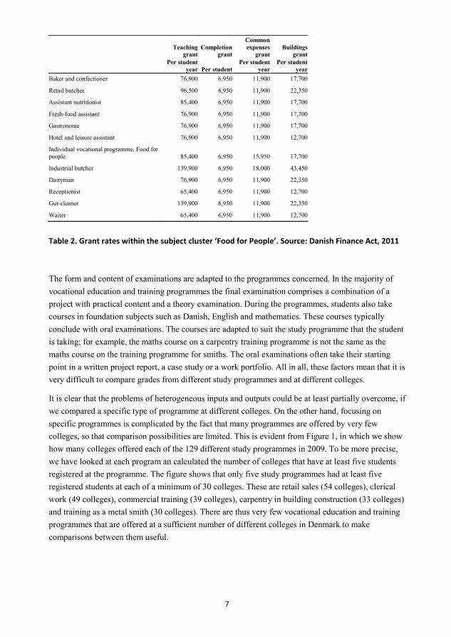
Table 2. Grant rates within the subject cluster ‘Food for People’. Source: Danish Finance Act, 2011

The form and content of examinations are adapted to the programmes concerned. In the majority of vocational education and training programmes the final examination comprises a combination of a project with practical content and a theory examination. During the programmes, students also take courses in foundation subjects such as Danish, English and mathematics. These courses typically conclude with oral examinations. The courses are adapted to suit the study programme that the student is taking; for example, the maths course on a carpentry training programme is not the same as the maths course on the training programme for smiths. The oral examinations often take their starting point in a written project report, a case study or a work portfolio. All in all, these factors mean that it is very difficult to compare grades from different study programmes and at different colleges.

It is clear that the problems of heterogeneous inputs and outputs could be at least partially overcome, if we compared a specific type of programme at different colleges. On the other hand, focusing on specific programmes is complicated by the fact that many programmes are offered by very few colleges, so that comparison possibilities are limited. This is evident from Figure 1, in which we show how many colleges offered each of the 129 different study programmes in 2009. To be more precise, we have looked at each program an calculated the number of colleges that have at least five students registered at the programme. The figure shows that only five study programmes had at least five registered students at each of a minimum of 30 colleges. These are retail sales (54 colleges), clerical work (49 colleges), commercial training (39 colleges), carpentry in building construction (33 colleges) and training as a metal smith (30 colleges). There are thus very few vocational education and training programmes that are offered at a sufficient number of different colleges in Denmark to make comparisons between them useful.

Virtually all the technical and commercial colleges offer both vocational education and training programmes and vocationally-oriented upper-secondary school courses. The colleges are self-governing institutions; the majority are in private self-ownership, though some are in the state sector. In recent years, there have been many amalgamations, and the number of vocational colleges in Denmark has halved during the past 15 years. This has not led to fewer physical locations for teaching vocational programmes, but rather to a reduction in the number of administrative units.

Vocational cluster 2002 2003 2004 2005 2006 2007 2008 2009 2010 2011 2012

Health, care and education 13,396 15,244 15,524 16,155 15,552 14,577 1,397 16,318 20,679 20,977 1,962

Motor vehicles, aircraft and other forms of transport

4,553 4,619 4,649 4,766 4,917 5,174 5,437 5,446 5,393 5,268 5,711

Building and construction 11,669 11,733 1,171 12,415 13,532 1,478 15,061 13,516 11,757 10,783 10,954

Building and user services 354 309 689 559 499 439 565 454 623 884 1,033

Animals, plants and nature 1,859 1,907 1,996 2,058 2,217 2,244 2,642 3,908 4,514 4,761 4,817

Commerce and office 18,077 17,584 16,889 16,752 17,768 18,364 17,773 1,546 15,623 16,896 17,268

Body and style 1,653 1,576 1,408 1,512 1,687 1,916 2,179 2,311 2,212 1,934 1,719

Food for people 6,332 6,198 6,037 5,847 5,695 5,548 5,261 5,051 5,222 5,453 5,866

Media production 1,586 1,538 1,263 1,262 1,365 1,397 1,546 1,811 1,923 2,005 2,017

Production and development

6,993 7,028 6,317 6,074 5,757 6,045 6,138 6,135 5,747 5,361 5,386

Power, control and IT 7,538 7,495 7,144 6,563 6,248 6,267 6,694, 643 5,843 5,457 5,429

Transport and logistics 1,279 1,446 1,539 1,568 1,674 1,812 193 1,952 2,042 2,356 2,396

Total 75,289 76,677 75,165 75,531 76,911 78,563 79,196 78,792 81,578 82,135 82,216

Table 1. Number of students enrolled in major subject clusters as of 30 September in various years.

Source: Danish Ministry of Education, Uni-C data bank

Vocational colleges are financed in the same way as upper-secondary schools, with a basic grant, a grant related to activities and a grant linked to the number of students who complete their programmes. The system of grants is, however, rather complex; for example, there are 48 different grant rates for operating costs. There is no correspondence between subject clusters and rates of grants. All clusters involve students taking major subjects, for which different grant rates apply. For example, within the ‘Food for People’ cluster, the grant rates vary from DKK 65,400 for training a waiter or receptionist up to 139,900 for training an industrial butcher or gut-cleaner; see Table 2.

7

Teaching grant

Completion grant

Common expenses

grantBuildings

grantPer student

year Per studentPer student

yearPer student

yearBaker and confectioner 76,900 6,950 11,900 17,700

Retail butcher 96,500 6,950 11,900 22,350

Assistant nutritionist 85,400 6,950 11,900 17,700

Fresh-food assistant 76,900 6,950 11,900 17,700

Gastronome 76,900 6,950 11,900 17,700

Hotel and leisure assistant 76,900 6,950 11,900 12,700

Individual vocational programme, Food for people 85,400 6,950 15,950 17,700

Industrial butcher 139,900 6,950 18,000 43,450

Dairyman 76,900 6,950 11,900 22,350

Receptionist 65,400 6,950 11,900 12,700

Gut-cleaner 139,900 6,950 11,900 22,350

Waiter 65,400 6,950 11,900 12,700

Table 2. Grant rates within the subject cluster ‘Food for People’. Source: Danish Finance Act, 2011

The form and content of examinations are adapted to the programmes concerned. In the majority of vocational education and training programmes the final examination comprises a combination of a project with practical content and a theory examination. During the programmes, students also take courses in foundation subjects such as Danish, English and mathematics. These courses typically conclude with oral examinations. The courses are adapted to suit the study programme that the student is taking; for example, the maths course on a carpentry training programme is not the same as the maths course on the training programme for smiths. The oral examinations often take their starting point in a written project report, a case study or a work portfolio. All in all, these factors mean that it is very difficult to compare grades from different study programmes and at different colleges.

It is clear that the problems of heterogeneous inputs and outputs could be at least partially overcome, if we compared a specific type of programme at different colleges. On the other hand, focusing on specific programmes is complicated by the fact that many programmes are offered by very few colleges, so that comparison possibilities are limited. This is evident from Figure 1, in which we show how many colleges offered each of the 129 different study programmes in 2009. To be more precise, we have looked at each program an calculated the number of colleges that have at least five students registered at the programme. The figure shows that only five study programmes had at least five registered students at each of a minimum of 30 colleges. These are retail sales (54 colleges), clerical work (49 colleges), commercial training (39 colleges), carpentry in building construction (33 colleges) and training as a metal smith (30 colleges). There are thus very few vocational education and training programmes that are offered at a sufficient number of different colleges in Denmark to make comparisons between them useful.

8

Figure 1. Distribution of the 129 Danish vocational education and training programmes according

to the number of colleges offering them and having at least five students enrolled on the

programmes, 2009

Focusing on specific courses is further complicated by the fact that from an accounting point of view, it is problematic to identify the costs connected to each programme. One possibility is obviously to assume that the taxi-meter rates correctly indicate resource expenditure. Another possibility would be to group programmes together, allowing comparison of a group of programmes across colleges. However, this is no easy task either, given that it first requires identification of groups of programmes, followed by determination of the key financial figures at group level. The Danish Education Ministry has attempted this in its ‘resource accounts’ project, but after five years of development work and the expenditure of DKK 36 million the project was abandoned in 2012 (see for example Sandal (2012)).

Using colleges as the unit for analysis makes it easier to identify resources expended. Comparing colleges has the disadvantage, however, that different colleges offer different combinations of training programmes, and it is easier to generate a positive effect from training in some programmes than in others. A college offering many courses for which it is easy to generate positive effects can thus appear in a highly favourable light in such comparisons. Nevertheless, we can overcome this problem to a considerable degree by using conditional results indicators – i.e. by accepting that, for example, the graduates from different programmes have differing prospects for employment, and then calculating each college’s contribution relative to the general employment prospects for the programmes that the college offers.

For these reasons, we decided in the first instance to use colleges as the units for analysis, but we do not exclude the possibility that benchmarking specific programmes may also be relevant in the future. In particular, it might be useful to carry out analyses of the five programmes which have at least five students enrolled at each of at least 30 colleges, namely retail sales, clerical work, commercial training, carpentry in building construction and training as a metal smith.

3. Resource and effects measurements It is normal to distinguish between effectiveness and efficiency analyses. Effectiveness analyses compare the goal of an activity with the actual effect that the activity has, while an efficiency analysis focuses more narrowly on comparing input (resource use) with the output produced (services), an efficient organisation being one that uses least input for most output. Productivity is a measure of the development over time.

In general it is difficult to measure both the goals of an activity and its final effects, and therefore it is more common to analyse efficiency than effectiveness. However, the taxi-meter system for the upper-secondary level in Denmark (including vocational education and training) means that it is slightly less useful to conduct efficiency analyses in this area. With the fixed grants per student, the taxi-meter system determines the efficiency of educational institutions to a high degree, in that there is a relationship between the number of students on the one hand and both income and expenditure on the other. For this reason, we have chosen to concentrate on analyses that include measurements of effects, both in the form of pure effectiveness analyses, in which indicators of effects are used as output, and in the form of advanced efficiency analyses that include a measurement of effects through the establishment of comparison groups.

A good effectiveness analysis requires ideally the inclusion of all resources and the identification of all relevant services and effects delivered. Thus, we are looking for complete descriptions. It is also important that there is a clear correspondence between input and output. The calculation of resources should not include elements that are used for purposes other than the measured output. Similarly, the measurement of services provided must not include output that derives from resources other than those recorded on the input side. In practice it is almost impossible to achieve this ideal, especially whenresearchers have to base their calculations on pre-existing data rather than having the opportunity to arrange the collection and standardisation of data for the specific purpose of benchmarking. It is therefore necessary to make do with using a variety of indicators to measure the input resources and the output and effects delivered.

Table 3 provides examples of possible inputs and outputs. A distinction is made here between analyses at the aggregated level, in which input and/or output are stated in the most condensed form possible, and disaggregated analyses, in which input and/or output are described in more detail. The advantage of using aggregated models is that they make it easier to find a correspondence between input and output. The quality of the data is probably also higher at the aggregated level than at the disaggregated level, because at the more detailed level various accounting distribution keys, etc. can generate artificial differences. On the other hand, disaggregated analyses have the advantage that they allow better understanding of the differences in the activities of the various institutions, and thus also distinguish the more productive institutions from the less productive ones. If the data available are of high quality, it is therefore more useful to apply disaggregated analyses.

9

Figure 1. Distribution of the 129 Danish vocational education and training programmes according

to the number of colleges offering them and having at least five students enrolled on the

programmes, 2009

Focusing on specific courses is further complicated by the fact that from an accounting point of view, it is problematic to identify the costs connected to each programme. One possibility is obviously to assume that the taxi-meter rates correctly indicate resource expenditure. Another possibility would be to group programmes together, allowing comparison of a group of programmes across colleges. However, this is no easy task either, given that it first requires identification of groups of programmes, followed by determination of the key financial figures at group level. The Danish Education Ministry has attempted this in its ‘resource accounts’ project, but after five years of development work and the expenditure of DKK 36 million the project was abandoned in 2012 (see for example Sandal (2012)).

Using colleges as the unit for analysis makes it easier to identify resources expended. Comparing colleges has the disadvantage, however, that different colleges offer different combinations of training programmes, and it is easier to generate a positive effect from training in some programmes than in others. A college offering many courses for which it is easy to generate positive effects can thus appear in a highly favourable light in such comparisons. Nevertheless, we can overcome this problem to a considerable degree by using conditional results indicators – i.e. by accepting that, for example, the graduates from different programmes have differing prospects for employment, and then calculating each college’s contribution relative to the general employment prospects for the programmes that the college offers.

For these reasons, we decided in the first instance to use colleges as the units for analysis, but we do not exclude the possibility that benchmarking specific programmes may also be relevant in the future. In particular, it might be useful to carry out analyses of the five programmes which have at least five students enrolled at each of at least 30 colleges, namely retail sales, clerical work, commercial training, carpentry in building construction and training as a metal smith.

3. Resource and effects measurements It is normal to distinguish between effectiveness and efficiency analyses. Effectiveness analyses compare the goal of an activity with the actual effect that the activity has, while an efficiency analysis focuses more narrowly on comparing input (resource use) with the output produced (services), an efficient organisation being one that uses least input for most output. Productivity is a measure of the development over time.

In general it is difficult to measure both the goals of an activity and its final effects, and therefore it is more common to analyse efficiency than effectiveness. However, the taxi-meter system for the upper-secondary level in Denmark (including vocational education and training) means that it is slightly less useful to conduct efficiency analyses in this area. With the fixed grants per student, the taxi-meter system determines the efficiency of educational institutions to a high degree, in that there is a relationship between the number of students on the one hand and both income and expenditure on the other. For this reason, we have chosen to concentrate on analyses that include measurements of effects, both in the form of pure effectiveness analyses, in which indicators of effects are used as output, and in the form of advanced efficiency analyses that include a measurement of effects through the establishment of comparison groups.

A good effectiveness analysis requires ideally the inclusion of all resources and the identification of all relevant services and effects delivered. Thus, we are looking for complete descriptions. It is also important that there is a clear correspondence between input and output. The calculation of resources should not include elements that are used for purposes other than the measured output. Similarly, the measurement of services provided must not include output that derives from resources other than those recorded on the input side. In practice it is almost impossible to achieve this ideal, especially whenresearchers have to base their calculations on pre-existing data rather than having the opportunity to arrange the collection and standardisation of data for the specific purpose of benchmarking. It is therefore necessary to make do with using a variety of indicators to measure the input resources and the output and effects delivered.

Table 3 provides examples of possible inputs and outputs. A distinction is made here between analyses at the aggregated level, in which input and/or output are stated in the most condensed form possible, and disaggregated analyses, in which input and/or output are described in more detail. The advantage of using aggregated models is that they make it easier to find a correspondence between input and output. The quality of the data is probably also higher at the aggregated level than at the disaggregated level, because at the more detailed level various accounting distribution keys, etc. can generate artificial differences. On the other hand, disaggregated analyses have the advantage that they allow better understanding of the differences in the activities of the various institutions, and thus also distinguish the more productive institutions from the less productive ones. If the data available are of high quality, it is therefore more useful to apply disaggregated analyses.

10

Level Aggregated Disaggregated

Resources used (input) Total costs Listing of numbers of employees, buildings used, etc.

or or

Total costs to the state (taxi-meter payments)

Costs of salaries, other operating costs, capital costs, etc.

Services provided (output) Increase in students’ skills/academic level Retention rate

Increases in students’ skills/academic level in different subjects, and possibly for different groups of students.

Post-course employment rate and rate of entry to higher education

Retention rates for different programmes.Post-course employment rates for students from different programmes

Table 3. Possible inputs and outputs in models of vocational education and training programmes

As far as the input side is concerned, it is unfortunately difficult in the case of vocational programmes to ensure that disaggregated calculations are accurate. This is because the units for inputs are higher level umbrella institutions which can cover several sub-institutions and types of educational programme. The problem affects both financial key figures, as reported in the Ministry of Education accounts database, and the numbers of personnel employed, etc., which are recorded by Statistics Denmark. On the input side, therefore, we have based our assessment of resource use on aggregated calculations.4 In order to ensure that there is a correspondence between input and output, we have been obliged to limit the number of vocational colleges used in the comparisons. The reason for this is that resource use accounting is carried out at the level of umbrella organisational institutions, while student characteristics are reported for the lower organisational level of sub-institutions. We have chosen to approach this problem with caution, and in the first instance5 we have included only the 39 vocational colleges where we can directly ensure that there is correspondence between resource use and student impact calculations. In those analyses which do not draw directly on resource use data we have instead used data from 66 vocational colleges. The colleges included in these analyses are listed in Table 4 below.

4 The analyses are based on register data for all Danish students who sat examinations in the period 2002-13 at upper-secondary schools, or who completed upper-secondary level courses. We have also obtained data from Statistics Denmark on the personnel employed at educational institutions, including information concerning their educational background, seniority and gender. Finally, we have used information on the financial situation of upper-secondary level educational institutions from the Ministry of Education database and from Statistics Denmark.

5 As mentioned previously, the Appendix presents corresponding analyses for a group of vocational education and training institutions for which we have used weighted student effects at the higher level of umbrella organisations. The sample used consists of over 60 institutions. The results of the two analyses are generally very similar.

39-college dataset 66-college dataset

København Nord SOPU KøbenhavnErhvervsskolen Nordsjælland København NordKøge Handelsskole SOPU NordsjællandRoskilde Handelsskole Erhvervsskolen NordsjællandCELF - Center for erhv.rettede udd. Lolland-Falster SOSU Sjælland GreveCampus Bornholm Køge HandelsskoleVestfyns Handelsskole og Handelsgymnasium Slagteriskolen i RoskildeKold College Roskilde HandelsskoleSyddansk Erhvervsskole Odense-Vejle Social- og Sundhedsskolen VestsjællandGråsten Landbrugsskole EUC NordvestsjællandHaderslev Handelsskole EUC LollandTønder Handelsskole SOSU Nykøbing F.Kjærgård Landbrugsskole SOSU Sjælland NæstvedEUC Vest CELF - Center for erhv.rettede udd. Lolland-FalsterGrindsted Landbrugsskole Bornholms Sundheds- og SygeplejeskoleErhvervsgymnasiet Grindsted Campus BornholmHandelsgymnasiet Ribe Vestfyns Handelsskole og HandelsgymnasiumVejen Business College Kold CollegeEUC Lillebælt Odense Tekniske SkoleBygholm Landbrugsskole Syddansk Erhvervsskole Odense-VejleLearnmark Horsens Gråsten LandbrugsskoleHANSENBERG Haderslev HandelsskoleCampus Vejle Tønder HandelsskoleAgroskolen Hammerum Social- og Sundhedsskolen SydLemvig Gymnasium; STX; HHX og HG Kjærgård LandbrugsskoleRingkjøbing Handelsskole & Handelsgymnasium EUC VestVestjydsk Handelsskole & Handelsgymnasium Rybners Erhverv HGDen jydske Haandværkerskole Social- og Sundhedsskolen EsbjergTradium tekniske erhvervsuddannelser og HTX Grindsted LandbrugsskoleTeknisk Skole Silkeborg Erhvervsgymnasiet GrindstedHandelsskolen Silkeborg Handelsgymnasiet RibeAARHUS TECH Varde Handelsskole og HandelsgymnasiumUddannelsesCenter Ringkøbing-Skjern Vejen Business CollegeSkive Tekniske Skole EUC LillebæltSkive Handelsskole Bygholm LandbrugsskoleAsmildkloster Landbrugsskole Learnmark HorsensFrederikshavn Handelsskole HANSENBERGNordjyllands Landbrugsskole Vejle Tekniske SkoleErhvervsskolerne Aars Campus Vejle

Agroskolen HammerumSocial & SundhedsSkolen; HerningHolstebro HandelsskoleLemvig Gymnasium; STX; HHX og HGRingkjøbing Handelsskole & HandelsgymnasiumUddannelsesCenter Ringkøbing-Skjern teknisk skoleVestjydsk Handelsskole & HandelsgymnasiumDen jydske HaandværkerskoleTradium tekniske erhvervsuddannelser og HTXRanders Social- og SundhedsskoleTeknisk Skole SilkeborgHandelsskolen SilkeborgSocial- og Sundhedsskolen i SilkeborgDansk Center for JordbrugsuddannelseAARHUS TECHÅrhus Social- og SundhedsskoleUddannelsesCenter Ringkøbing-SkjernSkive Tekniske SkoleSkive HandelsskoleAsmildkloster LandbrugsskoleEUC MIDTMercantec; Vinkelvej afdelingEUC NordFrederikshavn HandelsskoleNordjyllands LandbrugsskoleAMU NordjyllandErhvervsskolerne Aars

Table 4. Vocational colleges used in the primary analyses

11

Level Aggregated Disaggregated

Resources used (input) Total costs Listing of numbers of employees, buildings used, etc.

or or

Total costs to the state (taxi-meter payments)

Costs of salaries, other operating costs, capital costs, etc.

Services provided (output) Increase in students’ skills/academic level Retention rate

Increases in students’ skills/academic level in different subjects, and possibly for different groups of students.

Post-course employment rate and rate of entry to higher education

Retention rates for different programmes.Post-course employment rates for students from different programmes

Table 3. Possible inputs and outputs in models of vocational education and training programmes

As far as the input side is concerned, it is unfortunately difficult in the case of vocational programmes to ensure that disaggregated calculations are accurate. This is because the units for inputs are higher level umbrella institutions which can cover several sub-institutions and types of educational programme. The problem affects both financial key figures, as reported in the Ministry of Education accounts database, and the numbers of personnel employed, etc., which are recorded by Statistics Denmark. On the input side, therefore, we have based our assessment of resource use on aggregated calculations.4 In order to ensure that there is a correspondence between input and output, we have been obliged to limit the number of vocational colleges used in the comparisons. The reason for this is that resource use accounting is carried out at the level of umbrella organisational institutions, while student characteristics are reported for the lower organisational level of sub-institutions. We have chosen to approach this problem with caution, and in the first instance5 we have included only the 39 vocational colleges where we can directly ensure that there is correspondence between resource use and student impact calculations. In those analyses which do not draw directly on resource use data we have instead used data from 66 vocational colleges. The colleges included in these analyses are listed in Table 4 below.

4 The analyses are based on register data for all Danish students who sat examinations in the period 2002-13 at upper-secondary schools, or who completed upper-secondary level courses. We have also obtained data from Statistics Denmark on the personnel employed at educational institutions, including information concerning their educational background, seniority and gender. Finally, we have used information on the financial situation of upper-secondary level educational institutions from the Ministry of Education database and from Statistics Denmark.

5 As mentioned previously, the Appendix presents corresponding analyses for a group of vocational education and training institutions for which we have used weighted student effects at the higher level of umbrella organisations. The sample used consists of over 60 institutions. The results of the two analyses are generally very similar.

39-college dataset 66-college dataset

København Nord SOPU KøbenhavnErhvervsskolen Nordsjælland København NordKøge Handelsskole SOPU NordsjællandRoskilde Handelsskole Erhvervsskolen NordsjællandCELF - Center for erhv.rettede udd. Lolland-Falster SOSU Sjælland GreveCampus Bornholm Køge HandelsskoleVestfyns Handelsskole og Handelsgymnasium Slagteriskolen i RoskildeKold College Roskilde HandelsskoleSyddansk Erhvervsskole Odense-Vejle Social- og Sundhedsskolen VestsjællandGråsten Landbrugsskole EUC NordvestsjællandHaderslev Handelsskole EUC LollandTønder Handelsskole SOSU Nykøbing F.Kjærgård Landbrugsskole SOSU Sjælland NæstvedEUC Vest CELF - Center for erhv.rettede udd. Lolland-FalsterGrindsted Landbrugsskole Bornholms Sundheds- og SygeplejeskoleErhvervsgymnasiet Grindsted Campus BornholmHandelsgymnasiet Ribe Vestfyns Handelsskole og HandelsgymnasiumVejen Business College Kold CollegeEUC Lillebælt Odense Tekniske SkoleBygholm Landbrugsskole Syddansk Erhvervsskole Odense-VejleLearnmark Horsens Gråsten LandbrugsskoleHANSENBERG Haderslev HandelsskoleCampus Vejle Tønder HandelsskoleAgroskolen Hammerum Social- og Sundhedsskolen SydLemvig Gymnasium; STX; HHX og HG Kjærgård LandbrugsskoleRingkjøbing Handelsskole & Handelsgymnasium EUC VestVestjydsk Handelsskole & Handelsgymnasium Rybners Erhverv HGDen jydske Haandværkerskole Social- og Sundhedsskolen EsbjergTradium tekniske erhvervsuddannelser og HTX Grindsted LandbrugsskoleTeknisk Skole Silkeborg Erhvervsgymnasiet GrindstedHandelsskolen Silkeborg Handelsgymnasiet RibeAARHUS TECH Varde Handelsskole og HandelsgymnasiumUddannelsesCenter Ringkøbing-Skjern Vejen Business CollegeSkive Tekniske Skole EUC LillebæltSkive Handelsskole Bygholm LandbrugsskoleAsmildkloster Landbrugsskole Learnmark HorsensFrederikshavn Handelsskole HANSENBERGNordjyllands Landbrugsskole Vejle Tekniske SkoleErhvervsskolerne Aars Campus Vejle

Agroskolen HammerumSocial & SundhedsSkolen; HerningHolstebro HandelsskoleLemvig Gymnasium; STX; HHX og HGRingkjøbing Handelsskole & HandelsgymnasiumUddannelsesCenter Ringkøbing-Skjern teknisk skoleVestjydsk Handelsskole & HandelsgymnasiumDen jydske HaandværkerskoleTradium tekniske erhvervsuddannelser og HTXRanders Social- og SundhedsskoleTeknisk Skole SilkeborgHandelsskolen SilkeborgSocial- og Sundhedsskolen i SilkeborgDansk Center for JordbrugsuddannelseAARHUS TECHÅrhus Social- og SundhedsskoleUddannelsesCenter Ringkøbing-SkjernSkive Tekniske SkoleSkive HandelsskoleAsmildkloster LandbrugsskoleEUC MIDTMercantec; Vinkelvej afdelingEUC NordFrederikshavn HandelsskoleNordjyllands LandbrugsskoleAMU NordjyllandErhvervsskolerne Aars

Table 4. Vocational colleges used in the primary analyses

12

Resource useThe datasets we have created allow access to various indicators of resources used.

The taxi-meter grant is viewed as a particularly sound indicator in this context. It is also possible to argue that from a societal viewpoint it is the most relevant input. In socioeconomic terms, the crucial issue is what is achieved, and what it costs. How institutions use their resources is less important, provided they deliver value for money. We therefore believe that in principle, the taxi-meter-based analyses are the ones that are of the highest quality. The disaggregated calculations are also interesting, especially for learning purposes, and we therefore also want to present analyses using them; however, it is important to be aware that the basis for these analyses is less reliable. Disaggregated information can also be used in post-analyses (second stage analyses), in which any relationship found between effectiveness and specific choices made in the combination of inputs is analysed.

A simple variant on the idea of using taxi-meter grants as input is the notion of unit costs. As we saw previously, the students enrolled on the various training programmes trigger a variety of taxi-meter grants, and we can assume that these grants reflect real costs to a reasonably high degree. Assuming then that study programmes which attract the same grants have roughly the same efficient costs, we can expect it to be reasonable to compare the results generated by these various programmes without looking too closely at what they cost. In other words, we can assume that all programs have the same unit costs. Another benefit of using unit costs is that any taxi-meter grants for student completion of programmes will not make colleges which are good at taking students through their programmes to completion appear ineffective. It is after all a political aim that students should complete their studies.

In some of the analyses we have also taken into account disaggregated information about colleges’ resource usage. This mainly concerns wage costs or FTE (Full Time Equivalent) work years used for teaching and other purposes (e.g. administration). The calculations of these indicators are considered to be rather less reliable, but they are nonetheless useful as an illustration of what can be achieved with standardised calculations of resources and procedures used at the individual institutions. By including such information, it is possible to examine in more depth the reasons why some colleges perform better than others – is it, for example, that they do not have a large enough number of students, or because the administration is too large (or too small)?

The obligation to maintain anonymity (and the requirement that there should be at least five students enrolled in the relevant groups) in connection with the register data mean that unfortunately, there are a number of interesting characteristics that cannot always be identified. If colleges were to choose independently to share data in connection with benchmarking – as is common practice in a number of other sectors – then there would probably be significantly better opportunities for mutual learning and for understanding the reasons for any ineffectiveness at a given college.

Table 5 provides an overview of the main resource indicators in the sample of 39 colleges, which we compare below.

Variable Av. SD Q1(25%) Q2(50%) Q3(75%) Numberof NAs

Number of students 1,213 1,289 305 821 1,614 0Study costs 68 84 0 18 124 0Teaching taxi-meter grant, DKK millions 61 67 15 36 77 0Common expenses grant, DKK millions 14 14 4 9 19 0Buildings taxi-meter grant, DKK millions 8 12 2 5 9 0Other operating income, DKK millions 5 13 0 0 5 0Special grants, DKK millions 3 3 0 1 3 0Accounting, DKK millions 2 3 0 1 3 0Other income, including consultancy provision, DKK millions

0 1 0 0 0 0

Total state grants, DKK millions 95 107 23 75 112 0Payments by students and other income, total, DKK millions 20 22 4 11 27 0Total wage costs, DKK millions 72 78 18 53 92 0Wage costs, teaching, DKK millions 55 62 13 34 72 0Other wage costs, DKK millions 17 17 5 12 21 0Total teaching costs, DKK millions 73 80 17 47 91 0Wage costs, management and administration, DKK millions 8 9 2 6 9 0Total management costs, DKK millions 12 14 4 8 14 0Total turnover, DKK millions 118 128 31 87 137 0Total operating costs, DKK millions 113 123 30 85 132 0Unit costs 1 0 1 1 1 0Total salary costs per student 62,034 11,233 54,807 60,766 68,472 0Teaching taxi-meter rate per student 53,412 11,248 44,950 50,939 60,139 0Direct teaching staff (Eteachers) 79 82 28 40 92 26Teaching staff (all) 112 102 40 80 160 15Average salary 431,862 57,236 411,356 424,724 440,796 15Proportion of men 0.60 0.12 0.54 0.60 0.67 15Average age 47 6 44 47 48 15Teachers with other background 8 2 7 8 10 33Teachers with vocational program background 30 7 25 32 35 31Teachers with short study program background 15 5 12 13 16 35Teachers with medium-length study program background 24 5 20 23 26 26Teachers with long study program background 41 18 24 38 58 20FTEs per student 1.09 4.56 0.10 0.18 0.26 10Retention probability, average student 0.52 0.12 0.46 0.50 0.56 0Employment probability, average student 0.71 0.03 0.70 0.72 0.72 0

Table 5. Summary information about the 39 vocational colleges. All variables are calculated as

weighted averages with weights corresponding to the students who were admitted to vocational

colleges in the years 2008-10 and who took examinations in the period 2009-13

Effects indicators On the output side it is, as mentioned previously, impossible to compare grades across the numerous vocational education and training programmes. It could also be argued that grades are simply a type of intermediate product in relation to the primary goal of the vocational college, namely to prepare young people for employment. We have therefore attempted to summarise the various impacts of the colleges in the form of two generally relevant effects, namely retention of students and employment of graduates.

Data processing began with the identification of all individuals who began vocational education and training programmes during the period 2002-13. It was then possible to link various items of background information to these individuals, including information about their parents, their results from primary/lower-secondary school and their progress at upper-secondary level. Some upper-secondary level institutions in Denmark enrol a large number of students who are rather older than the norm. In order to focus exclusively on the education of young people, for the purposes of the analyses we removed from the sample all students aged above 20 years at the commencement of their upper-

13

Resource useThe datasets we have created allow access to various indicators of resources used.

The taxi-meter grant is viewed as a particularly sound indicator in this context. It is also possible to argue that from a societal viewpoint it is the most relevant input. In socioeconomic terms, the crucial issue is what is achieved, and what it costs. How institutions use their resources is less important, provided they deliver value for money. We therefore believe that in principle, the taxi-meter-based analyses are the ones that are of the highest quality. The disaggregated calculations are also interesting, especially for learning purposes, and we therefore also want to present analyses using them; however, it is important to be aware that the basis for these analyses is less reliable. Disaggregated information can also be used in post-analyses (second stage analyses), in which any relationship found between effectiveness and specific choices made in the combination of inputs is analysed.

A simple variant on the idea of using taxi-meter grants as input is the notion of unit costs. As we saw previously, the students enrolled on the various training programmes trigger a variety of taxi-meter grants, and we can assume that these grants reflect real costs to a reasonably high degree. Assuming then that study programmes which attract the same grants have roughly the same efficient costs, we can expect it to be reasonable to compare the results generated by these various programmes without looking too closely at what they cost. In other words, we can assume that all programs have the same unit costs. Another benefit of using unit costs is that any taxi-meter grants for student completion of programmes will not make colleges which are good at taking students through their programmes to completion appear ineffective. It is after all a political aim that students should complete their studies.

In some of the analyses we have also taken into account disaggregated information about colleges’ resource usage. This mainly concerns wage costs or FTE (Full Time Equivalent) work years used for teaching and other purposes (e.g. administration). The calculations of these indicators are considered to be rather less reliable, but they are nonetheless useful as an illustration of what can be achieved with standardised calculations of resources and procedures used at the individual institutions. By including such information, it is possible to examine in more depth the reasons why some colleges perform better than others – is it, for example, that they do not have a large enough number of students, or because the administration is too large (or too small)?

The obligation to maintain anonymity (and the requirement that there should be at least five students enrolled in the relevant groups) in connection with the register data mean that unfortunately, there are a number of interesting characteristics that cannot always be identified. If colleges were to choose independently to share data in connection with benchmarking – as is common practice in a number of other sectors – then there would probably be significantly better opportunities for mutual learning and for understanding the reasons for any ineffectiveness at a given college.

Table 5 provides an overview of the main resource indicators in the sample of 39 colleges, which we compare below.

Variable Av. SD Q1(25%) Q2(50%) Q3(75%) Numberof NAs

Number of students 1,213 1,289 305 821 1,614 0Study costs 68 84 0 18 124 0Teaching taxi-meter grant, DKK millions 61 67 15 36 77 0Common expenses grant, DKK millions 14 14 4 9 19 0Buildings taxi-meter grant, DKK millions 8 12 2 5 9 0Other operating income, DKK millions 5 13 0 0 5 0Special grants, DKK millions 3 3 0 1 3 0Accounting, DKK millions 2 3 0 1 3 0Other income, including consultancy provision, DKK millions

0 1 0 0 0 0

Total state grants, DKK millions 95 107 23 75 112 0Payments by students and other income, total, DKK millions 20 22 4 11 27 0Total wage costs, DKK millions 72 78 18 53 92 0Wage costs, teaching, DKK millions 55 62 13 34 72 0Other wage costs, DKK millions 17 17 5 12 21 0Total teaching costs, DKK millions 73 80 17 47 91 0Wage costs, management and administration, DKK millions 8 9 2 6 9 0Total management costs, DKK millions 12 14 4 8 14 0Total turnover, DKK millions 118 128 31 87 137 0Total operating costs, DKK millions 113 123 30 85 132 0Unit costs 1 0 1 1 1 0Total salary costs per student 62,034 11,233 54,807 60,766 68,472 0Teaching taxi-meter rate per student 53,412 11,248 44,950 50,939 60,139 0Direct teaching staff (Eteachers) 79 82 28 40 92 26Teaching staff (all) 112 102 40 80 160 15Average salary 431,862 57,236 411,356 424,724 440,796 15Proportion of men 0.60 0.12 0.54 0.60 0.67 15Average age 47 6 44 47 48 15Teachers with other background 8 2 7 8 10 33Teachers with vocational program background 30 7 25 32 35 31Teachers with short study program background 15 5 12 13 16 35Teachers with medium-length study program background 24 5 20 23 26 26Teachers with long study program background 41 18 24 38 58 20FTEs per student 1.09 4.56 0.10 0.18 0.26 10Retention probability, average student 0.52 0.12 0.46 0.50 0.56 0Employment probability, average student 0.71 0.03 0.70 0.72 0.72 0

Table 5. Summary information about the 39 vocational colleges. All variables are calculated as

weighted averages with weights corresponding to the students who were admitted to vocational

colleges in the years 2008-10 and who took examinations in the period 2009-13

Effects indicators On the output side it is, as mentioned previously, impossible to compare grades across the numerous vocational education and training programmes. It could also be argued that grades are simply a type of intermediate product in relation to the primary goal of the vocational college, namely to prepare young people for employment. We have therefore attempted to summarise the various impacts of the colleges in the form of two generally relevant effects, namely retention of students and employment of graduates.

Data processing began with the identification of all individuals who began vocational education and training programmes during the period 2002-13. It was then possible to link various items of background information to these individuals, including information about their parents, their results from primary/lower-secondary school and their progress at upper-secondary level. Some upper-secondary level institutions in Denmark enrol a large number of students who are rather older than the norm. In order to focus exclusively on the education of young people, for the purposes of the analyses we removed from the sample all students aged above 20 years at the commencement of their upper-

14

It is therefore important to apply a statistical model that can correct for such differences in estimating the contribution of each individual college. We have used a multi-level model (Steele, 2009) to determine the probability of an ‘average student’ completing a programme at a given college.

Figure 2 shows the retention effects for vocational education and training programmes at around 100 colleges, calculated as the additive impact from the colleges on the probability of retention for the average student. The students analysed began their courses between 2008 and 2010. There are very significant differences among the colleges in their ability to retain the average student. In interpreting the retention effects of vocational education and training programmes, it is important to note that we have controlled for the differences that can be attributed to the different subject clusters. The retention rates for some clusters – the commercial cluster, for example – are higher than for others; however, the retention effects we report take into account the different levels in different clusters. On the other hand, the calculations do not take into account differences in the different programmes availablewithin the program clusters, and a low retention rate may be attributable to the combination of programmes offered by a given college. Nor do the calculations take into account the availability of workplace practical training places for each college. From a societal perspective, the indicator remains a useful tool for revealing colleges’ effectiveness, but it is obviously more difficult for some colleges than for others to improve their results.

Figure 2. Retention effects

secondary level education. Thus, colleges were evaluated solely on the results achieved with young people aged 20 or below at the start of their educational programmes.

It was important to include both retention percentages (completion percentages) and rate of employment after completion in the data, since it was thought that there might be a trade-off between the two indicators.

Completion percentages must be viewed in relation to the average national completion rates for the subject cluster concerned, and must take into account students’ socioeconomic background and scholastic level at the end of the ninth grade in lower-secondary school. This makes it possible to estimate for each training programme whether each college does better or worse than should be expected.

Employment rates must similarly be assessed in relation to the average or ‘normal’ rate of employment for the subject cluster concerned, again taking into account students’ socioeconomic backgrounds and scholastic achievement in the ninth grade.

Retention rate As described in detail in Wittrup, Jacobsen and Andersen (2014), there are correlations between drop-out rate and both socioeconomic factors and scholastic level at primary/lower-secondary school. School grades in mathematics and physics are of particular importance, in that students who achieve good grades in these topics are significantly less likely to drop out. In addition, the probability of students dropping out of vocational college increases if their parents do not live together, and if they come from non-Western families. The effects are shown in the regression table below.

Variable Coefficient t value p value Retention probability, % High grade (76 or more) in written maths 0.2207 10.00 0.000 74.60 High grade (7 or more) in physics/chemistry 0.1433 6.54 0.000 73.11 High grade (7 or more) in oral maths 0.0728 3.56 0.000 71.70 High grade (7 or more) in oral English -0.0801 -3.89 0.000 68.50 High grade (7 or more) in Danish written presentation 0.0575 3.25 0.001 71.39 High grade (7 or more) in Danish spelling -0.1021 -3.54 0.000 68.02 No lower-secondary school grades -0.4623 -13.80 0.000 59.74 Parents not cohabiting -0.3260 -21.90 0.000 62.97 Non-Western origin -0.3215 -11.99 0.000 63.07 Non-Danish Western origin -0.2011 -4.07 0.000 65.83 Girl 0.0988 5.37 0.000 72.22 Each additional year of student’s age at programme start -0.0770 -4.70 0.000 68.56 Father in high income group 0.0286 8.35 0.000 70.79 Mother in high income group 0.0261 7.42 0.000 70.74 Each additional 10 points higher status of father’s job (SIOPS) -0.0354 -5.09 0.000 69.45 Father self-employed 0.1920 6.54 0.000 74.05 Mother self-employed 0.2448 5.90 0.000 75.06 Mother is senior executive 0.1334 4.45 0.000 72.91 Mother is drawing unemployment benefit 0.1197 5.56 0.000 72.64 School-friends in higher level on social index 0.3987 7.32 0.000 77.83

6 A grade of 7 represents the third level down (‘good’) on the ‘7-step’ Danish academic grading scale, and is thus above average.

15

It is therefore important to apply a statistical model that can correct for such differences in estimating the contribution of each individual college. We have used a multi-level model (Steele, 2009) to determine the probability of an ‘average student’ completing a programme at a given college.

Figure 2 shows the retention effects for vocational education and training programmes at around 100 colleges, calculated as the additive impact from the colleges on the probability of retention for the average student. The students analysed began their courses between 2008 and 2010. There are very significant differences among the colleges in their ability to retain the average student. In interpreting the retention effects of vocational education and training programmes, it is important to note that we have controlled for the differences that can be attributed to the different subject clusters. The retention rates for some clusters – the commercial cluster, for example – are higher than for others; however, the retention effects we report take into account the different levels in different clusters. On the other hand, the calculations do not take into account differences in the different programmes availablewithin the program clusters, and a low retention rate may be attributable to the combination of programmes offered by a given college. Nor do the calculations take into account the availability of workplace practical training places for each college. From a societal perspective, the indicator remains a useful tool for revealing colleges’ effectiveness, but it is obviously more difficult for some colleges than for others to improve their results.

Figure 2. Retention effects

16

Variable Coefficient t value p valueProbability ofbeing inemployment, %

No lower-secondary school grades -1.0087 -17.03 0.000 56.02High grade (7 or more) in physics/chemistry 0.2038 5.21 0.000 81.07High grade (7 or more) in Danish spelling 0.1595 3.78 0.000 80.38High grade (7 or more) in mathematical problem-solving 0.1444 3.58 0.000 80.14

Low grade (4 or less) in Danish written presentation -0.1069 -3.11 0.002 75.84

Student one year older than normal at programme start -0.0996 -7.49 0.000 75.97

Father in high income group 0.0490 7.23 0.000 78.58Non-Western origin -0.3600 -6.24 0.000 70.91Mother is senior executive 0.2267 3.70 0.000 81.42Each additional year in age of mother at student’s birth 0.0130 3.26 0.001 77.97

Mother self-employed 0.2696 3.19 0.001 82.06Each additional year in age of father at student’s birth -0.0098 -2.97 0.003 77.57

School-friends in higher level on social index -0.3306 -2.70 0.007 71.51Mother is drawing unemployment benefit 0.1194 2.69 0.007 79.74

Table 7. Regression model for explaining the probability of being in employment after completing a

vocational education and training programme. Comparisons with the median student’s probability

of being in employment of 77.74%

To evaluate colleges’ success in getting their students into employment, it is therefore necessary to correct for differences in students’ backgrounds. We have calculated an employment effect that identifies the impact on subsequent employment that can be attributed to the work of the college.Figure 3 shows the distribution of the employment effects of around 100 colleges, calculated as theadditive impact from the colleges on the probability of employment for the average student. As the confidence intervals indicate, there is a significant degree of uncertainty associated with these measurements.

Figure 3. Employment effects

Employment Employment is an important parameter by which to assess vocational education and training programmes, and it is described as a central goal of such programmes in the relevant legislation (Consolidated Act of Parliament No. 439 of 29.04.2013). According to Section 1, vocational education and training programmes must give young people an education that provides the basis for their future employment, and must meet the needs of the labour market with respect to both trade and general qualifications (Section 1, Subsection 2). It is thus Danish policy that vocational colleges, unlike upper-secondary schools, should provide their students with skills that are immediately usable on the labour market. At the same time, the training programmes must be responsive to the needs of the labour market. Efforts are made to ensure this through the organisational setup, with the parties to the labour market being strongly represented on the boards of vocational colleges. It seems self-evident that both employers and employees will have no hesitation in agreeing that employment is a central goal for the colleges.

As described in Jacobsen & Wittrup (2014), we again used individual-level data from Statistics Denmark to examine students’ rates of employment. We identified the students who commenced their vocational education and training programmes in or after 2002 and completed them by 2010 at the latest. As with the other analyses, we included only students aged 20 years or less at the start of their study. We then determined whether the former students were in employment one year after completing their vocational education and training programmes. If students were enrolled in higher education or were on parental leave, we decided to count them as being ‘in employment’.

The analysis shows that students who achieved good results in the lower-secondary school leaving examinations in the ninth grade were more likely find employment after completing vocational education and training. It is noticeable that students who did not have a lower-secondary leaving examination with grades had particular difficulty in finding a job. Social background variables also continue to be of significance after the completion of the training programme. In particular, it seems that students from non-Western families, students whose fathers have low incomes and students who began their training programme relatively late in life have greater difficulty in finding work. The effects are shown in the regression table (Table 7) below.7

7 Only variables that are significant at the 99% level are shown in the table.

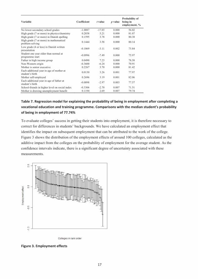
17

Variable Coefficient t value p valueProbability ofbeing inemployment, %

No lower-secondary school grades -1.0087 -17.03 0.000 56.02High grade (7 or more) in physics/chemistry 0.2038 5.21 0.000 81.07High grade (7 or more) in Danish spelling 0.1595 3.78 0.000 80.38High grade (7 or more) in mathematical problem-solving 0.1444 3.58 0.000 80.14

Low grade (4 or less) in Danish written presentation -0.1069 -3.11 0.002 75.84

Student one year older than normal at programme start -0.0996 -7.49 0.000 75.97

Father in high income group 0.0490 7.23 0.000 78.58Non-Western origin -0.3600 -6.24 0.000 70.91Mother is senior executive 0.2267 3.70 0.000 81.42Each additional year in age of mother at student’s birth 0.0130 3.26 0.001 77.97

Mother self-employed 0.2696 3.19 0.001 82.06Each additional year in age of father at student’s birth -0.0098 -2.97 0.003 77.57

School-friends in higher level on social index -0.3306 -2.70 0.007 71.51Mother is drawing unemployment benefit 0.1194 2.69 0.007 79.74

Table 7. Regression model for explaining the probability of being in employment after completing a

vocational education and training programme. Comparisons with the median student’s probability

of being in employment of 77.74%

To evaluate colleges’ success in getting their students into employment, it is therefore necessary to correct for differences in students’ backgrounds. We have calculated an employment effect that identifies the impact on subsequent employment that can be attributed to the work of the college.Figure 3 shows the distribution of the employment effects of around 100 colleges, calculated as theadditive impact from the colleges on the probability of employment for the average student. As the confidence intervals indicate, there is a significant degree of uncertainty associated with these measurements.

Figure 3. Employment effects

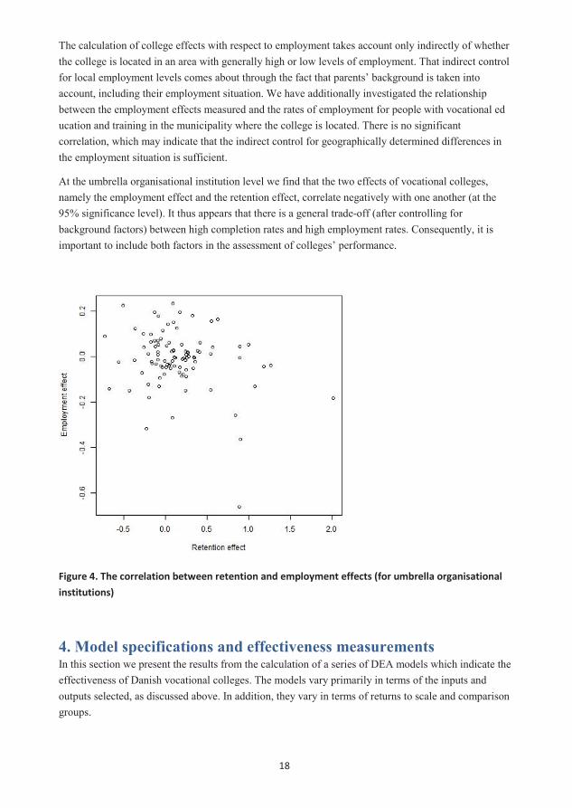
18

The calculation of college effects with respect to employment takes account only indirectly of whether the college is located in an area with generally high or low levels of employment. That indirect control for local employment levels comes about through the fact that parents’ background is taken into account, including their employment situation. We have additionally investigated the relationship between the employment effects measured and the rates of employment for people with vocational education and training in the municipality where the college is located. There is no significant correlation, which may indicate that the indirect control for geographically determined differences in the employment situation is sufficient.

At the umbrella organisational institution level we find that the two effects of vocational colleges, namely the employment effect and the retention effect, correlate negatively with one another (at the 95% significance level). It thus appears that there is a general trade-off (after controlling for background factors) between high completion rates and high employment rates. Consequently, it is important to include both factors in the assessment of colleges’ performance.

Figure 4. The correlation between retention and employment effects (for umbrella organisational

institutions)

4. Model specifications and effectiveness measurementsIn this section we present the results from the calculation of a series of DEA models which indicate the effectiveness of Danish vocational colleges. The models vary primarily in terms of the inputs and outputs selected, as discussed above. In addition, they vary in terms of returns to scale and comparison groups.

Returns to scale In addition to inputs and outputs, it is necessary to include in the model set-ups an assumption concerning returns to scale. Returns to scale refers here to the way in which the size of a college affects the costs per unit produced. The most important assumptions are:

• Variable returns to scale (VRS), where there may be disadvantages in being either too large or too small an institution

• Increasing returns to scale (IRS), where it may be a disadvantage to be too small an institution

• Constant returns to scale (CRS), where there is no significant disadvantage in being either a large or a small institution.

If the model operates with costs per student, we can apply equivalent assumptions, though the interpretation of the results is naturally a little different. CRS, for example, would mean that there is no marginal increase in costs associated with increasing retention rate, even when the retention rate is already high.

We have tested the various possible assumptions concerning returns to scale in all cases, and used the assumptions best supported by the data. We also believe that the resulting assumptions concerning returns to scale make good sense intuitively.

Comparison groups Benchmarking involves making comparisons with the aim of assessing the position of a given institution in relation to those institutions which provide the basis for the comparison. Consequently, the choice of institutions with which to make comparisons is a key issue.

A fundamental principle in all DEA models is that a given institution should be compared only with another institution or a combination of other institutions which have used at most the same resources to produce at least the same level of services as the institution being compared. This requirement applies for every input and every output.

This simple principle has proved to be highly practicable and has contributed to ensuring effective, data-based identification of relevant comparable institutions. Traditional DEA analyses are based solely on this comparison requirement.

However, we go further and implement additional institution-specific restrictions on the comparisons involved. In this regard, we use the principles presented in Table 8.

Group Definition All Relevant to compare all institutions Employment effect Relevant to make comparisons with institutions which have at least the same employment

effect Retention effect Relevant to make comparisons with institutions which have at least the same level of

retention

Table 8. Comparison groups

19

The calculation of college effects with respect to employment takes account only indirectly of whether the college is located in an area with generally high or low levels of employment. That indirect control for local employment levels comes about through the fact that parents’ background is taken into account, including their employment situation. We have additionally investigated the relationship between the employment effects measured and the rates of employment for people with vocational education and training in the municipality where the college is located. There is no significant correlation, which may indicate that the indirect control for geographically determined differences in the employment situation is sufficient.

At the umbrella organisational institution level we find that the two effects of vocational colleges, namely the employment effect and the retention effect, correlate negatively with one another (at the 95% significance level). It thus appears that there is a general trade-off (after controlling for background factors) between high completion rates and high employment rates. Consequently, it is important to include both factors in the assessment of colleges’ performance.

Figure 4. The correlation between retention and employment effects (for umbrella organisational

institutions)

4. Model specifications and effectiveness measurementsIn this section we present the results from the calculation of a series of DEA models which indicate the effectiveness of Danish vocational colleges. The models vary primarily in terms of the inputs and outputs selected, as discussed above. In addition, they vary in terms of returns to scale and comparison groups.

Returns to scale In addition to inputs and outputs, it is necessary to include in the model set-ups an assumption concerning returns to scale. Returns to scale refers here to the way in which the size of a college affects the costs per unit produced. The most important assumptions are:

• Variable returns to scale (VRS), where there may be disadvantages in being either too large or too small an institution

• Increasing returns to scale (IRS), where it may be a disadvantage to be too small an institution

• Constant returns to scale (CRS), where there is no significant disadvantage in being either a large or a small institution.

If the model operates with costs per student, we can apply equivalent assumptions, though the interpretation of the results is naturally a little different. CRS, for example, would mean that there is no marginal increase in costs associated with increasing retention rate, even when the retention rate is already high.

We have tested the various possible assumptions concerning returns to scale in all cases, and used the assumptions best supported by the data. We also believe that the resulting assumptions concerning returns to scale make good sense intuitively.

Comparison groups Benchmarking involves making comparisons with the aim of assessing the position of a given institution in relation to those institutions which provide the basis for the comparison. Consequently, the choice of institutions with which to make comparisons is a key issue.

A fundamental principle in all DEA models is that a given institution should be compared only with another institution or a combination of other institutions which have used at most the same resources to produce at least the same level of services as the institution being compared. This requirement applies for every input and every output.

This simple principle has proved to be highly practicable and has contributed to ensuring effective, data-based identification of relevant comparable institutions. Traditional DEA analyses are based solely on this comparison requirement.

However, we go further and implement additional institution-specific restrictions on the comparisons involved. In this regard, we use the principles presented in Table 8.

Group Definition All Relevant to compare all institutions Employment effect Relevant to make comparisons with institutions which have at least the same employment

effect Retention effect Relevant to make comparisons with institutions which have at least the same level of

retention

Table 8. Comparison groups

20

Quantitative models with qualitative restrictions We analysed a number of quantitative models with qualitative restrictions, and these are presented in Table 9.

Model Input: Costs Output: Students Comparison group Returns to scale

A Teaching taxi-meter grant Students High employment and retention effects IRS

B1 Total wage costs Students High employment and retention effects IRS

B2 Wage costs, teaching Wage costs, other Students High employment and retention effects IRS

C1 Total FTEs Students High employment and retention effects IRS

C2 FTEs, teaching FTEs, other Students High employment and retention effects IRS

Table 9. Quantitative models in which the output is the number of students

In all the models in Table 9, the output is the number of students. Input is calculated in three different ways. The most highly aggregated measure of input is the total teaching taxi-meter grant (A). One alternative approach is to use total wage costs (B1) or total FTEs worked (C1) at the associated institutions. Finally, there are two more disaggregated models in which wage costs and FTEs are divided up into those resources which are directly linked to teaching and those which are related to support functions (B2 and C2). There is reason to expect that the correspondence between input and output will be best in the A model, next best in the B models and poorest in the C models.

Furthermore, the FTE models (C1 and C2) fail to capture variations in the quality of the various types of employees, such as those that may be evidenced by a higher wage level.

It must be emphasised that quantitative models will penalise colleges that teach very resource-demanding programmes. In socioeconomic terms, the taxi-meter and the FTE approaches are particularly useful if, at the same time, we can calculate the societal benefit of the various educational programmes and thus perform a true cost-benefit analysis. Since, however, we are unable to do this, we can instead assume that all the different educational programmes are of equal socioeconomic value. If we do so, then the quantitative models are equivalent to a ‘value for money’ approach; that is to say, we ask what society gets from each Danish krone spent, and make comparisons with the colleges that train the greatest number of students for the resources expended.

In all cases, efficiency is calculated in such a way that no institution is compared with others unless those other institutions display a greater level of effectiveness in terms of retention and employment. It is thus not possible for an institution to appear particularly cost-efficient by compromising on quality.

Note that all the models are based on increasing (non-diminishing) returns to scale. We thus assume that there may be extra costs (per student) involved in being a small institution, but not in being a large institution. The data support this assumption, which also makes good intuitive sense in relation to normal production models, since an institution which experiences diminishing returns to scale should, in principle, be able to reorganise itself into several smaller units.

The application of these additional restrictions leads to more conservative results, which naturally then means that the potentials for improvements are reduced.

In the case of institutions for which there is a very small comparison group, the results can be significantly skewed. This is intuitively evident; such institutions are ‘competing’ with very few others and therefore have a greater chance of being among the best. However, it is possible to correct statistically for this skewness in order to ensure fair and useful comparisons. This is done by using bootstrapping, which allows us to calculate bias-corrected efficiency results.

5. Results All the results are calculated for the students who enrolled at Danish vocational colleges during the period 2008-10, and who took examinations during the period 2009-13. However, the employment effects calculated are for students who enrolled in 2005 and onwards. In order to create the best possible correspondence between inputs and outputs, all measurements of costs are calculated in the same way: the years 2008-13 are weighted in proportion to their relative use of resources for the student group identified, taking into account the resource data which were available at the time the calculations were made – primarily information for the period 2008-11.8

Note that it is not clear how well the resource accounting, which is by the calendar year, matches the study programme information, which is for the academic year; nor is it clear when exactly a given student received teaching in the course of a multi-year programme. For reasons of caution, we have decided to focus on average values over a period using three student cohorts. The shorter we set the limits, the more that random variations in examination results will impact on the results of the analysis. Since best practice analyses generally derive their usefulness from differences in output from given resource use, and since resources presumably cannot be adjusted precisely from year to year, the choice of a short analysis period would cause the apparent potential for improvement to be larger. Colleges which have a particularly good outcome in a given year will show up as a role model in calculations made for that year, but not necessarily in other years.9

The models used can be divided into two groups, namely quantitative models with qualitative restrictions and effect models. In all cases, returns to scale are determined by statistical tests and with the requirement that they should be conceptually reasonable.

8 The resource calculations we have used are based on data from the Ministry of Education accounts database, which contains information about taxi-meter grants and student numbers, and from Statistics Denmark, from whom we have obtained information on work years, educational background, seniority, etc. Some of the resource characteristics were only used for a post-analysis (second stage) check of whether efficiencies varied with these characteristics.

9 This does not necessarily mean that single year analyses are without interest. If, for example, it makes a difference which teacher teaches students in a given year, then that is certainly useful to know. Variations from one year to another in an institution’s efficiency will thus provide information on internal possibilities for learning best practice from other teachers in the same institution, and comparisons between institutions can now be interpreted as opportunities to learn best practice by learning from other institutions and their teachers.

21

Quantitative models with qualitative restrictions We analysed a number of quantitative models with qualitative restrictions, and these are presented in Table 9.

Model Input: Costs Output: Students Comparison group Returns to scale

A Teaching taxi-meter grant Students High employment and retention effects IRS

B1 Total wage costs Students High employment and retention effects IRS

B2 Wage costs, teaching Wage costs, other Students High employment and retention effects IRS

C1 Total FTEs Students High employment and retention effects IRS

C2 FTEs, teaching FTEs, other Students High employment and retention effects IRS

Table 9. Quantitative models in which the output is the number of students

In all the models in Table 9, the output is the number of students. Input is calculated in three different ways. The most highly aggregated measure of input is the total teaching taxi-meter grant (A). One alternative approach is to use total wage costs (B1) or total FTEs worked (C1) at the associated institutions. Finally, there are two more disaggregated models in which wage costs and FTEs are divided up into those resources which are directly linked to teaching and those which are related to support functions (B2 and C2). There is reason to expect that the correspondence between input and output will be best in the A model, next best in the B models and poorest in the C models.

Furthermore, the FTE models (C1 and C2) fail to capture variations in the quality of the various types of employees, such as those that may be evidenced by a higher wage level.

It must be emphasised that quantitative models will penalise colleges that teach very resource-demanding programmes. In socioeconomic terms, the taxi-meter and the FTE approaches are particularly useful if, at the same time, we can calculate the societal benefit of the various educational programmes and thus perform a true cost-benefit analysis. Since, however, we are unable to do this, we can instead assume that all the different educational programmes are of equal socioeconomic value. If we do so, then the quantitative models are equivalent to a ‘value for money’ approach; that is to say, we ask what society gets from each Danish krone spent, and make comparisons with the colleges that train the greatest number of students for the resources expended.

In all cases, efficiency is calculated in such a way that no institution is compared with others unless those other institutions display a greater level of effectiveness in terms of retention and employment. It is thus not possible for an institution to appear particularly cost-efficient by compromising on quality.

Note that all the models are based on increasing (non-diminishing) returns to scale. We thus assume that there may be extra costs (per student) involved in being a small institution, but not in being a large institution. The data support this assumption, which also makes good intuitive sense in relation to normal production models, since an institution which experiences diminishing returns to scale should, in principle, be able to reorganise itself into several smaller units.

22

Summary results for these models are presented in Table 10. The various models are described in different rows. The numbers of institutions included are given. It is generally the case that efficiencies fall with the number of observations, because there are more instances to compare with, and because achieving best practice in a large group, all else being equal, is more demanding than achieving it in a small group.

After the numbers of observations, two alternative measures of efficiency are given. The first, ‘Efficiency’, is directly calculated as the individual institutions’ efficiency in relation to the institution-specific comparison groups. The other efficiency measurement is the ‘Bias corrected’ measurement. For each institution we have calculated by how much the measurement of efficiency is overestimated because of the limited size of the comparison group. For both measures of efficiency, the table provides an average value, the standard deviation and the 25, 50 and 75 percentiles of the distribution.

For example, in Model B2 we see that the average efficiency is 0.91. This means that if the average institution adopted best practice, it would be able to save 9% of wage costs with the given number of students, without any detrimental effect on retention or employment rates. We can also see that 25 percent of institutions could save at least 17 percent (1-0.83). When we correct for bias, the potentials for improvement increase by 10-15 percentage points.

The models thus estimate average efficiencies of between 0.73 and 0.91 percent, equivalent to improvement potentials of between 9 and 27 percent. Improvement potentials can be interpreted, as above, as possible proportional savings in input. Given that at a local level there are probably constant returns to scale, they can also be viewed as an approximate expression of potential additional student admissions through the application of best practice without the expenditure of additional resources. Improvement potentials of this magnitude in a group of under 40 institutions are by no means insignificant. The improvement potential should actually be viewed as even larger, insofar as normal DEA analyses do not apply restrictions with regard to quality; in other words, we have been especially cautious in our calculation of efficiencies.

Model Number of Efficiency Bias-corrected efficiency

observations Av. SD 25% 50% 75% Av. SD 25% 50% 75%

A 39 0.82 0.14 0.74 0.82 0.96 0.67 0.14 0.61 0.71 0.74

B1 39 0.88 0.14 0.80 0.94 1.00 0.77 0.18 0.65 0.80 0.92

B2 39 0.91 0.13 0.83 0.99 1.00 0.82 0.14 0.71 0.90 0.93

C1 29 0.73 0.31 0.44 0.88 1.00

C2 13 0.82 0.25 0.61 1.00 1.00

Table 10. Efficiencies in the quantitative models

If we compare the B1 and B2 results (or the C1 and C2 results), we see that the disaggregated models indicate higher efficiencies than the aggregated ones. The difference is the allocative inefficiency, the amount which colleges could save by making an optimal allocation of staffing costs between staff

directly involved in teaching and support personnel. The differences are not large in the most reliable of the models, namely model B, but insofar as the data are of sufficiently high quality, a comparison ofC1 and C2 indicates that on average staff costs are around 9 percent higher if colleges do not find the optimal allocation of expenditure on personnel. Some colleges appear to have too many support staff, and others too few.

Effect modelsThe models described below are effect models. Table 11 provides an overview. In all the effect models, the focus is on the retention effect, the employment effect, or both. This focus is achieved in part through the specification of the output, and in part through the choice of comparison groups. In the final classes of model (F, F1 and F2), where both effects are regarded as output, we seek to find a combination of institutions which have on average at least the same retention effect and employment effect. This means that some of the role model colleges that contribute to the average may have a lower educational effect than the institution being evaluated, but there are others that have a greater effect, so that the average dominates the evaluated institution. In this sense, the limitations on quality in this class of model are a little less restrictive than in the quantitative models.

The inputs in all these models are an expression of the resources used per student. The resources used are expressed either as taxi-meter grants or salary costs. In addition, we have used the most aggregated expression of resources used, namely unit costs.

The returns to scale in these models are variable (VRS). This means that it may be relatively expensive to increase effectiveness, and that it may be very difficult to raise retention or employmenteffects above certain levels.

Model Input: Costs per student Output: Effect Comparison group Returns to scale

D Unit costs Employment effect Higher retention effect VRS

D1 Taxi-meter grants per student Employment effect Higher retention effect VRS

D2 Total wage costs per student Employment effect Higher retention effect VRS

E Unit costs Retention effect Higher employment effect VRS

E1 Taxi-meter grants per student Retention effect Higher employment effect VRS

E2 Total wage costs per student Retention effect Higher employment effect VRS

F Unit costs Employment effect + retention effect All VRS

F1 Taxi-meter grants per student Employment effect + retention effect All VRS

F2 Total wage costs per student Employment effect + retention effect All VRS

Table 11. Effect models, where outputs are employment and retention effects

Summary results for the effect models are presented in Table 12. The form of the table and the interpretation of the figures are the same as in Table 10. The comparison groups in these models are generally rather larger than those used in the pure quantitative models, because there are now no

23

Summary results for these models are presented in Table 10. The various models are described in different rows. The numbers of institutions included are given. It is generally the case that efficiencies fall with the number of observations, because there are more instances to compare with, and because achieving best practice in a large group, all else being equal, is more demanding than achieving it in a small group.

After the numbers of observations, two alternative measures of efficiency are given. The first, ‘Efficiency’, is directly calculated as the individual institutions’ efficiency in relation to the institution-specific comparison groups. The other efficiency measurement is the ‘Bias corrected’ measurement. For each institution we have calculated by how much the measurement of efficiency is overestimated because of the limited size of the comparison group. For both measures of efficiency, the table provides an average value, the standard deviation and the 25, 50 and 75 percentiles of the distribution.

For example, in Model B2 we see that the average efficiency is 0.91. This means that if the average institution adopted best practice, it would be able to save 9% of wage costs with the given number of students, without any detrimental effect on retention or employment rates. We can also see that 25 percent of institutions could save at least 17 percent (1-0.83). When we correct for bias, the potentials for improvement increase by 10-15 percentage points.

The models thus estimate average efficiencies of between 0.73 and 0.91 percent, equivalent to improvement potentials of between 9 and 27 percent. Improvement potentials can be interpreted, as above, as possible proportional savings in input. Given that at a local level there are probably constant returns to scale, they can also be viewed as an approximate expression of potential additional student admissions through the application of best practice without the expenditure of additional resources. Improvement potentials of this magnitude in a group of under 40 institutions are by no means insignificant. The improvement potential should actually be viewed as even larger, insofar as normal DEA analyses do not apply restrictions with regard to quality; in other words, we have been especially cautious in our calculation of efficiencies.

Model Number of Efficiency Bias-corrected efficiency

observations Av. SD 25% 50% 75% Av. SD 25% 50% 75%

A 39 0.82 0.14 0.74 0.82 0.96 0.67 0.14 0.61 0.71 0.74

B1 39 0.88 0.14 0.80 0.94 1.00 0.77 0.18 0.65 0.80 0.92

B2 39 0.91 0.13 0.83 0.99 1.00 0.82 0.14 0.71 0.90 0.93

C1 29 0.73 0.31 0.44 0.88 1.00

C2 13 0.82 0.25 0.61 1.00 1.00

Table 10. Efficiencies in the quantitative models

If we compare the B1 and B2 results (or the C1 and C2 results), we see that the disaggregated models indicate higher efficiencies than the aggregated ones. The difference is the allocative inefficiency, the amount which colleges could save by making an optimal allocation of staffing costs between staff

directly involved in teaching and support personnel. The differences are not large in the most reliable of the models, namely model B, but insofar as the data are of sufficiently high quality, a comparison ofC1 and C2 indicates that on average staff costs are around 9 percent higher if colleges do not find the optimal allocation of expenditure on personnel. Some colleges appear to have too many support staff, and others too few.

Effect modelsThe models described below are effect models. Table 11 provides an overview. In all the effect models, the focus is on the retention effect, the employment effect, or both. This focus is achieved in part through the specification of the output, and in part through the choice of comparison groups. In the final classes of model (F, F1 and F2), where both effects are regarded as output, we seek to find a combination of institutions which have on average at least the same retention effect and employment effect. This means that some of the role model colleges that contribute to the average may have a lower educational effect than the institution being evaluated, but there are others that have a greater effect, so that the average dominates the evaluated institution. In this sense, the limitations on quality in this class of model are a little less restrictive than in the quantitative models.

The inputs in all these models are an expression of the resources used per student. The resources used are expressed either as taxi-meter grants or salary costs. In addition, we have used the most aggregated expression of resources used, namely unit costs.

The returns to scale in these models are variable (VRS). This means that it may be relatively expensive to increase effectiveness, and that it may be very difficult to raise retention or employmenteffects above certain levels.

Model Input: Costs per student Output: Effect Comparison group Returns to scale

D Unit costs Employment effect Higher retention effect VRS

D1 Taxi-meter grants per student Employment effect Higher retention effect VRS

D2 Total wage costs per student Employment effect Higher retention effect VRS

E Unit costs Retention effect Higher employment effect VRS

E1 Taxi-meter grants per student Retention effect Higher employment effect VRS

E2 Total wage costs per student Retention effect Higher employment effect VRS

F Unit costs Employment effect + retention effect All VRS

F1 Taxi-meter grants per student Employment effect + retention effect All VRS

F2 Total wage costs per student Employment effect + retention effect All VRS

Table 11. Effect models, where outputs are employment and retention effects

Summary results for the effect models are presented in Table 12. The form of the table and the interpretation of the figures are the same as in Table 10. The comparison groups in these models are generally rather larger than those used in the pure quantitative models, because there are now no

24

limitations on retention and employment effects. This means that, all else being equal, we should expect slightly lower efficiencies. On the other hand, the efficiencies are now dependent in part on how much the college effects – now the output – vary. This means that insofar as the multi-level models of retention and employment effects are able to explain a large part of the variation through socioeconomic conditions, the college effects will also be limited, and consequently the variations in the output in the effect models. This will tend towards giving higher efficiencies, simply because the analyses will indicate that the efforts of the institutions only affect students to a limited extent.

If we focus on the employment effect, it seems that on average it is possible to improve the proportion of former students in employment by around five percent in the most cautious scenario. In this context, all institutions are assumed to have the same expenditures per student (D). The average potentials are somewhat larger with respect to improving retention without compromising on employment; the average improvement in this case is around 25 percent.

We see that savings potentials are generally larger when we use taxi-meter costs per student or wage costs per student at the individual institutions. There are several possible explanations for this. One is that the calculation of wage costs does not correspond perfectly with the calculations related to students, thus introducing an ‘artificial’ variation that is captured in the best practice model as a difference in efficiency. Another is that some colleges are better at employing staff who will make a positive contribution to retention and employment. A final and more obvious explanation is simply that some colleges offer a greater number of costly programmes, so that in reality these additional savings cannot be achieved.

Model Number of Efficiency Bias-corrected efficiency

observations Av. SD 25% 50% 75% Av. SD 25% 50% 75%

D 66 0.95 0.04 0.93 0.95 0.97 0.94 0.04 0.93 0.94 0.96

D 39 0.96 0.04 0.94 0.96 0.99 0.95 0.02 0.94 0.96 0.97

D1 39 0.74 0.17 0.59 0.72 0.88 0.59 0.18 0.46 0.58 0.74

D2 39 0.82 0.15 0.71 0.82 0.99 0.70 0.20 0.60 0.70 0.89

E 66 0.74 0.15 0.65 0.72 0.85 0.69 0.16 0.61 0.68 0.78

E 39 0.73 0.17 0.64 0.71 0.81 0.65 0.18 0.55 0.65 0.71

E1 39 0.72 0.18 0.57 0.65 0.87 0.50 0.18 0.41 0.51 0.59

E2 39 0.76 0.15 0.68 0.76 0.84 0.59 0.14 0.52 0.62 0.71

F 66 0.95 0.03 0.93 0.95 0.97 0.94 0.03 0.93 0.94 0.97

F 39 0.96 0.03 0.94 0.95 0.98 0.95 0.03 0.93 0.95 0.96

F1 39 0.69 0.17 0.56 0.65 0.79 0.52 0.18 0.44 0.54 0.66

F2 39 0.75 0.15 0.66 0.73 0.81 0.61 0.14 0.52 0.65 0.73

Table 12. Efficiencies in the effect models

Concretization of the potentials In order to concretize the potentials for improvement, it can be useful to bear in mind that the probability of former students being in employment among the 39 (66) vocational colleges is 0.72 (0.70), while the average retention rate among the 39 (66) vocational colleges is 0.52 (0.52). A five percent increase in the employment effect, as in Model D, would mean that average employment would increase in round figures from 72 percent to 1.05*0.72 = 0.76 = 76 percent. Similarly, a 27 percent improvement in retention, as in Model E, would mean an increase from 52 percent to 1.27* 0.52 = 0.66 = 66 percent.

These figures are only approximate, for two reasons. First, the efficiencies are calculated as input efficiencies, not output efficiencies. In other words, the efficiency calculations represent potential savings in resources used. As returns to scale are not constant, there is no complete symmetry between what can be saved on the input side and what can be improved on the output side. The second reason that the potentials can only be calculated approximately in this way is that units with greater potential for improvement will tend to be those with low retention and employment effects. This means that the average savings percentage cannot be applied equally to all units.

In those models which use unit costs, the efficiencies can be interpreted directly as the proportional savings in unit costs that are necessary to achieve effective, best-practice operation. In the other models, it is possible to state a monetary amount using the same system. In model D1, for example, where we calculate an efficiency of 0.74, this can be interpreted as meaning that the taxi-meter grant could be reduced from DKK 53,412 per student in the colleges analysed to 0.74*53,412 = DKK 39,525 per student, i.e. a saving per student of DKK 13,887 per year. With a total of 47,307 students attending the colleges in the analysis, this represents a potential annual saving of DKK 657 million. If, instead of calculating average savings potentials and average taxi-meter values, we calculate specific savings, college by college, we arrive at a division of savings potentials as shown in Figure 5. Here we can see that 17 colleges could save between DKK 0 and 5 million, seven colleges between 5 and 10 million, and so on. The potential total socioeconomic savings in this case can be calculated as being DKK 602 million. If, finally, we consider that our analyses only cover around one third of all students at vocational colleges, and if we assume that the colleges analysed are reasonably representative of all such colleges, we find that the calculated efficiency of 0.74 in Model D1 would represent a potential saving in excess of DKK 1.5-2 billion at vocational colleges.

25

limitations on retention and employment effects. This means that, all else being equal, we should expect slightly lower efficiencies. On the other hand, the efficiencies are now dependent in part on how much the college effects – now the output – vary. This means that insofar as the multi-level models of retention and employment effects are able to explain a large part of the variation through socioeconomic conditions, the college effects will also be limited, and consequently the variations in the output in the effect models. This will tend towards giving higher efficiencies, simply because the analyses will indicate that the efforts of the institutions only affect students to a limited extent.

If we focus on the employment effect, it seems that on average it is possible to improve the proportion of former students in employment by around five percent in the most cautious scenario. In this context, all institutions are assumed to have the same expenditures per student (D). The average potentials are somewhat larger with respect to improving retention without compromising on employment; the average improvement in this case is around 25 percent.

We see that savings potentials are generally larger when we use taxi-meter costs per student or wage costs per student at the individual institutions. There are several possible explanations for this. One is that the calculation of wage costs does not correspond perfectly with the calculations related to students, thus introducing an ‘artificial’ variation that is captured in the best practice model as a difference in efficiency. Another is that some colleges are better at employing staff who will make a positive contribution to retention and employment. A final and more obvious explanation is simply that some colleges offer a greater number of costly programmes, so that in reality these additional savings cannot be achieved.

Model Number of Efficiency Bias-corrected efficiency

observations Av. SD 25% 50% 75% Av. SD 25% 50% 75%

D 66 0.95 0.04 0.93 0.95 0.97 0.94 0.04 0.93 0.94 0.96

D 39 0.96 0.04 0.94 0.96 0.99 0.95 0.02 0.94 0.96 0.97

D1 39 0.74 0.17 0.59 0.72 0.88 0.59 0.18 0.46 0.58 0.74

D2 39 0.82 0.15 0.71 0.82 0.99 0.70 0.20 0.60 0.70 0.89

E 66 0.74 0.15 0.65 0.72 0.85 0.69 0.16 0.61 0.68 0.78

E 39 0.73 0.17 0.64 0.71 0.81 0.65 0.18 0.55 0.65 0.71

E1 39 0.72 0.18 0.57 0.65 0.87 0.50 0.18 0.41 0.51 0.59

E2 39 0.76 0.15 0.68 0.76 0.84 0.59 0.14 0.52 0.62 0.71

F 66 0.95 0.03 0.93 0.95 0.97 0.94 0.03 0.93 0.94 0.97

F 39 0.96 0.03 0.94 0.95 0.98 0.95 0.03 0.93 0.95 0.96

F1 39 0.69 0.17 0.56 0.65 0.79 0.52 0.18 0.44 0.54 0.66

F2 39 0.75 0.15 0.66 0.73 0.81 0.61 0.14 0.52 0.65 0.73

Table 12. Efficiencies in the effect models

Concretization of the potentials In order to concretize the potentials for improvement, it can be useful to bear in mind that the probability of former students being in employment among the 39 (66) vocational colleges is 0.72 (0.70), while the average retention rate among the 39 (66) vocational colleges is 0.52 (0.52). A five percent increase in the employment effect, as in Model D, would mean that average employment would increase in round figures from 72 percent to 1.05*0.72 = 0.76 = 76 percent. Similarly, a 27 percent improvement in retention, as in Model E, would mean an increase from 52 percent to 1.27* 0.52 = 0.66 = 66 percent.

These figures are only approximate, for two reasons. First, the efficiencies are calculated as input efficiencies, not output efficiencies. In other words, the efficiency calculations represent potential savings in resources used. As returns to scale are not constant, there is no complete symmetry between what can be saved on the input side and what can be improved on the output side. The second reason that the potentials can only be calculated approximately in this way is that units with greater potential for improvement will tend to be those with low retention and employment effects. This means that the average savings percentage cannot be applied equally to all units.

In those models which use unit costs, the efficiencies can be interpreted directly as the proportional savings in unit costs that are necessary to achieve effective, best-practice operation. In the other models, it is possible to state a monetary amount using the same system. In model D1, for example, where we calculate an efficiency of 0.74, this can be interpreted as meaning that the taxi-meter grant could be reduced from DKK 53,412 per student in the colleges analysed to 0.74*53,412 = DKK 39,525 per student, i.e. a saving per student of DKK 13,887 per year. With a total of 47,307 students attending the colleges in the analysis, this represents a potential annual saving of DKK 657 million. If, instead of calculating average savings potentials and average taxi-meter values, we calculate specific savings, college by college, we arrive at a division of savings potentials as shown in Figure 5. Here we can see that 17 colleges could save between DKK 0 and 5 million, seven colleges between 5 and 10 million, and so on. The potential total socioeconomic savings in this case can be calculated as being DKK 602 million. If, finally, we consider that our analyses only cover around one third of all students at vocational colleges, and if we assume that the colleges analysed are reasonably representative of all such colleges, we find that the calculated efficiency of 0.74 in Model D1 would represent a potential saving in excess of DKK 1.5-2 billion at vocational colleges.

26

Figure 5. Potential savings in the education taxi-meter rates in DKK millions among 39 vocational

colleges

5. Conclusion The analyses show that vocational colleges vary considerably with respect to resource spending per student. This variation, and consequently the potentials for improvement, appear to be significantly larger for vocational colleges than for normal upper-secondary schools, as analysed in Bogetoft and Wittrup (2014). In this connection it should be borne in mind that the number of vocational colleges analysed was rather small. This means – especially for the ‘normal’ measurements of efficiency – that, all else being equal, the potentials for improvement among vocational colleges should have been lower, since fewer colleges were ‘competing’ with each other. On the other hand, the results are naturally dependent on which vocational colleges are selected for comparison. Furthermore, the model specifications for the vocational colleges analysis are different, in that we cannot use corrected grades to measure the educational advances among students at these colleges, making direct comparisons of results impossible.

If all the programmes are assumed to be of equal value to society, then average savings of 9-33% could be made without any reduction in the colleges’ retention of students or levels of employment among former students. The savings calculation is based on the assumption that the colleges adopt best practice and also change their course programme profiles, so that expensive programmes are replaced by less resource-demanding ones. This is indicated by the quantitative models A, B1, B2, C1 and C2.

If instead we assume that all programmes are in reality equally costly (or that their relevance for society is proportional to the taxi-meter grants allocated to them), then it is possible on average to save between 4 and 48 percent, as is indicated by the effect models, D, E and F. To be more precise, we can

say that on average it is possible to improve the employment effect by 5-6 percent without affecting retention, to improve retention by 31-35 percent without affecting the employment effect, and to improve both retention and employment by 5-6 percent without increasing costs and without changing the range of programmes that colleges offer.

It must also be emphasised that the average savings and improvement potentials often conceal the fact that a number of specific institutions have significant potentials for increasing efficiency. This is indicated by the percentiles. We have not presented results for individual colleges in this study paper, since it is not our intention to publicly pillory institutions, but readers who are interested in using the methods and results for learning purposes are welcome to contact the authors.10

Another interesting insight from these analyses concerns the data that are accessible. Undoubtedly, comprehensive data do exist in some areas. Denmark is in an almost unique position, for example, with regard to register-based information available for analyses concerning individuals. In other areas, however, our experience shows that there is a lack of standardised data. This is the case at institutional level, for example, where comparable data concerning resource use and organisation is of crucial importance for the evaluation of efficiency. If benchmarking and identification of best practice are to become systematised and form a natural part of management in institutions – both centrally and locally – it is vital that standardised accounting of resource use, etc. should be established.

10 Peter Bogetoft (pb.eco@cbs.dk) and Jesper Wittrup (JeWi@kora.dk).

27

Figure 5. Potential savings in the education taxi-meter rates in DKK millions among 39 vocational

colleges

5. Conclusion The analyses show that vocational colleges vary considerably with respect to resource spending per student. This variation, and consequently the potentials for improvement, appear to be significantly larger for vocational colleges than for normal upper-secondary schools, as analysed in Bogetoft and Wittrup (2014). In this connection it should be borne in mind that the number of vocational colleges analysed was rather small. This means – especially for the ‘normal’ measurements of efficiency – that, all else being equal, the potentials for improvement among vocational colleges should have been lower, since fewer colleges were ‘competing’ with each other. On the other hand, the results are naturally dependent on which vocational colleges are selected for comparison. Furthermore, the model specifications for the vocational colleges analysis are different, in that we cannot use corrected grades to measure the educational advances among students at these colleges, making direct comparisons of results impossible.

If all the programmes are assumed to be of equal value to society, then average savings of 9-33% could be made without any reduction in the colleges’ retention of students or levels of employment among former students. The savings calculation is based on the assumption that the colleges adopt best practice and also change their course programme profiles, so that expensive programmes are replaced by less resource-demanding ones. This is indicated by the quantitative models A, B1, B2, C1 and C2.

If instead we assume that all programmes are in reality equally costly (or that their relevance for society is proportional to the taxi-meter grants allocated to them), then it is possible on average to save between 4 and 48 percent, as is indicated by the effect models, D, E and F. To be more precise, we can

say that on average it is possible to improve the employment effect by 5-6 percent without affecting retention, to improve retention by 31-35 percent without affecting the employment effect, and to improve both retention and employment by 5-6 percent without increasing costs and without changing the range of programmes that colleges offer.

It must also be emphasised that the average savings and improvement potentials often conceal the fact that a number of specific institutions have significant potentials for increasing efficiency. This is indicated by the percentiles. We have not presented results for individual colleges in this study paper, since it is not our intention to publicly pillory institutions, but readers who are interested in using the methods and results for learning purposes are welcome to contact the authors.10

Another interesting insight from these analyses concerns the data that are accessible. Undoubtedly, comprehensive data do exist in some areas. Denmark is in an almost unique position, for example, with regard to register-based information available for analyses concerning individuals. In other areas, however, our experience shows that there is a lack of standardised data. This is the case at institutional level, for example, where comparable data concerning resource use and organisation is of crucial importance for the evaluation of efficiency. If benchmarking and identification of best practice are to become systematised and form a natural part of management in institutions – both centrally and locally – it is vital that standardised accounting of resource use, etc. should be established.

10 Peter Bogetoft (pb.eco@cbs.dk) and Jesper Wittrup (JeWi@kora.dk).

28

Appendix This appendix presents the results from parallel analyses we have conducted using data from over 60 colleges, as opposed to the under 40 colleges in the primary analyses. The larger dataset has been created by calculating the student effects for higher organisational level umbrella institutions as a weighted combination of the student effects at the sub-institutions for which we have data. The models and the analytical tools used are otherwise exactly the same as for the primary analyses.

The results of these supplementary analyses are very similar to those obtained with the primary analyses. Since the sample of colleges is somewhat larger, however, there is a tendency for the extended analyses to indicate lower efficiencies.

Data

Aalborg Handelsskole IBC International Business College

AARHUS TECH Jordbrugets UddannelsesCenter Århus

Agroskolen Hammerum Kjærgård Landbrugsskole

Århus Købmandsskole København Nord

Asmildkloster Landbrugsskole Københavns Tekniske Skole

Business College Syd Mommark HkS - Sønderborg HS Køge Handelsskole

Bygholm Landbrugsskole Kold College

Campus Bornholm Learnmark Horsens

Campus Vejle Lemvig Gymnasium; STX; HHX og HG

CELF - Center for erhv.rettede udd. Lolland-Falst Mercantec

CPH - Uddannelsescenter København Vest Niels Brock - Copenhagen Business College

Dalum Landbrugsskole Nordjyllands Landbrugsskole

Den jydske Haandværkerskole Ringkjøbing Handelsskole & Handelsgymnasium

Erhvervsgymnasiet Grindsted Roskilde Handelsskole

Erhvervsskolen Nordsjælland Roskilde Tekniske Skole

Erhvervsskolerne Aars Selandia – CEU

EUC Lillebælt Skanderborg-Odder Center for uddannelse

EUC Nord Skive Handelsskole

EUC Nordvestsjælland Skive Tekniske Skole

EUC Sjælland Svendborg Erhvervsskole

EUC Syd Syddansk Erhvervsskole Odense-Vejle

EUC Vest TEC Teknisk Erhvervsskole Center

Frederikshavn Handelsskole Tech College Aalborg

Gråsten Landbrugsskole Teknisk Skole Silkeborg

Grindsted Landbrugsskole TietgenSkolen

Haderslev Handelsskole Tønder Handelsskole

Handelsgymnasiet Ribe UddannelsesCenter Ringkøbing-Skjern

Handelsskolen Silkeborg Vejen Business College

HANSENBERG Vestfyns Handelsskole og Handelsgymnasium

Herningsholm Erhvervsskole Vestjydsk Handelsskole & Handelsgymnasium

Hotel- og Restaurantskolen Viden Djurs

Table 13. Vocational colleges used in the extended analyses

Model Number of Efficiency Bias-corrected efficiency

observations Av. SD 25% 50% 75% Av. SD 25% 50% 75%

A 62 0.77 0.17 0.66 0.78 0.91 0.62 0.17 0.49 0.63 0.74

B1 62 0.84 0.15 0.68 0.88 1.00 0.71 0.17 0.55 0.73 0.86

B2 62 0.87 0.15 0.72 0.94 1.00 0.72 0.16 0.59 0.72 0.88

C1 43 0.66 0.27 0.49 0.60 1.00

C2 20 0.83 0.28 0.58 1.00 1.00

Table 14. Efficiencies in the quantitative models in the extended analyses

Model Number of Efficiency Bias-corrected efficiency

observations Av. SD 25% 50% 75% Av. SD 25% 50% 75%

D 62 0.95 0.04 0.93 0.95 0.97 0.94 0.03 0.92 0.94 0.96

D1 62 0.70 0.18 0.56 0.64 0.83 0.55 0.18 0.42 0.54 0.65

D2 62 0.77 0.15 0.65 0.75 0.89 0.64 0.16 0.52 0.64 0.76

E 62 0.74 0.13 0.65 0.72 0.81 0.68 0.13 0.59 0.67 0.73

E1 62 0.69 0.17 0.56 0.65 0.81 0.54 0.18 0.45 0.54 0.64

E2 62 0.76 0.15 0.64 0.75 0.86 0.63 0.16 0.51 0.63 0.73

F 62 0.95 0.03 0.93 0.95 0.97 0.94 0.03 0.93 0.94 0.96

F1 62 0.68 0.17 0.56 0.64 0.75 0.53 0.17 0.41 0.53 0.65

F2 62 0.74 0.14 0.64 0.73 0.82 0.62 0.13 0.51 0.62 0.73

Table 15. Efficiencies in the effect models

29

Appendix This appendix presents the results from parallel analyses we have conducted using data from over 60 colleges, as opposed to the under 40 colleges in the primary analyses. The larger dataset has been created by calculating the student effects for higher organisational level umbrella institutions as a weighted combination of the student effects at the sub-institutions for which we have data. The models and the analytical tools used are otherwise exactly the same as for the primary analyses.

The results of these supplementary analyses are very similar to those obtained with the primary analyses. Since the sample of colleges is somewhat larger, however, there is a tendency for the extended analyses to indicate lower efficiencies.

Data

Aalborg Handelsskole IBC International Business College

AARHUS TECH Jordbrugets UddannelsesCenter Århus

Agroskolen Hammerum Kjærgård Landbrugsskole

Århus Købmandsskole København Nord

Asmildkloster Landbrugsskole Københavns Tekniske Skole

Business College Syd Mommark HkS - Sønderborg HS Køge Handelsskole

Bygholm Landbrugsskole Kold College

Campus Bornholm Learnmark Horsens

Campus Vejle Lemvig Gymnasium; STX; HHX og HG

CELF - Center for erhv.rettede udd. Lolland-Falst Mercantec

CPH - Uddannelsescenter København Vest Niels Brock - Copenhagen Business College

Dalum Landbrugsskole Nordjyllands Landbrugsskole

Den jydske Haandværkerskole Ringkjøbing Handelsskole & Handelsgymnasium

Erhvervsgymnasiet Grindsted Roskilde Handelsskole

Erhvervsskolen Nordsjælland Roskilde Tekniske Skole

Erhvervsskolerne Aars Selandia – CEU

EUC Lillebælt Skanderborg-Odder Center for uddannelse

EUC Nord Skive Handelsskole

EUC Nordvestsjælland Skive Tekniske Skole

EUC Sjælland Svendborg Erhvervsskole

EUC Syd Syddansk Erhvervsskole Odense-Vejle

EUC Vest TEC Teknisk Erhvervsskole Center

Frederikshavn Handelsskole Tech College Aalborg

Gråsten Landbrugsskole Teknisk Skole Silkeborg

Grindsted Landbrugsskole TietgenSkolen

Haderslev Handelsskole Tønder Handelsskole

Handelsgymnasiet Ribe UddannelsesCenter Ringkøbing-Skjern

Handelsskolen Silkeborg Vejen Business College

HANSENBERG Vestfyns Handelsskole og Handelsgymnasium

Herningsholm Erhvervsskole Vestjydsk Handelsskole & Handelsgymnasium

Hotel- og Restaurantskolen Viden Djurs

Table 13. Vocational colleges used in the extended analyses

Model Number of Efficiency Bias-corrected efficiency

observations Av. SD 25% 50% 75% Av. SD 25% 50% 75%

A 62 0.77 0.17 0.66 0.78 0.91 0.62 0.17 0.49 0.63 0.74

B1 62 0.84 0.15 0.68 0.88 1.00 0.71 0.17 0.55 0.73 0.86

B2 62 0.87 0.15 0.72 0.94 1.00 0.72 0.16 0.59 0.72 0.88

C1 43 0.66 0.27 0.49 0.60 1.00

C2 20 0.83 0.28 0.58 1.00 1.00

Table 14. Efficiencies in the quantitative models in the extended analyses

Model Number of Efficiency Bias-corrected efficiency

observations Av. SD 25% 50% 75% Av. SD 25% 50% 75%

D 62 0.95 0.04 0.93 0.95 0.97 0.94 0.03 0.92 0.94 0.96

D1 62 0.70 0.18 0.56 0.64 0.83 0.55 0.18 0.42 0.54 0.65

D2 62 0.77 0.15 0.65 0.75 0.89 0.64 0.16 0.52 0.64 0.76

E 62 0.74 0.13 0.65 0.72 0.81 0.68 0.13 0.59 0.67 0.73

E1 62 0.69 0.17 0.56 0.65 0.81 0.54 0.18 0.45 0.54 0.64

E2 62 0.76 0.15 0.64 0.75 0.86 0.63 0.16 0.51 0.63 0.73

F 62 0.95 0.03 0.93 0.95 0.97 0.94 0.03 0.93 0.94 0.96

F1 62 0.68 0.17 0.56 0.64 0.75 0.53 0.17 0.41 0.53 0.65

F2 62 0.74 0.14 0.64 0.73 0.82 0.62 0.13 0.51 0.62 0.73

Table 15. Efficiencies in the effect models

References Andersen, Lotte Bøgh, Peter Bogetoft, Jørgen Grønnegård Christensen and Torben Tranæs (eds) (2014). Styring, ledelse og resultater på ungdomsuddannelserne. Odense: Syddansk Universitetsforlag.

Bogetoft, Peter (2012). Performance benchmarking – Measuring and managing performance. New York: Springer.

Bogetoft, Peter, Eskil Heinesen and Torben Tranæs (2014). The efficiency of educational production: A comparison of Denmark with other OECD countries. Study Paper 71, Odense: University Press of Southern Denmark.

Bogetoft, Peter, Eskil Heinesen and Torben Tranæs (2014). ‘Internationale effektivitetsforskelle i uddannelsesproduktion’. Chapter 11 in Andersen et al. (2014).

Bogetoft, Peter, Ole Olesen and Niels Christian Petersen (1987). ‘Produktivitetsevaluering af 96 danske sygehuse – En præsentation af DEA-metoden og et eksempel på dens anvendelse’. Ledelse og Erhvervsøkonomi, 2: 67-81.

Bogetoft, Peter and Lars Otto (2011). Benchmarking with DEA, SFA, and R. New York: Springer.

Bogetoft, Peter and Jesper Wittrup (2011). ‘Productivity and education: Benchmarking of elementary and lower-secondary Schools in Denmark’. Nordic Economic Policy Review, 2: 257-294.

Bogetoft, Peter and Jesper Wittrup (2014). ‘Effektive skoler: Benchmarking af danske ungdomsuddannelsesinstitutioner med særlig fokus på gymnasierne’. Chapter 7 in Andersen et al. (2014).

Jennergren, L. Peter and Børge Obel (1986). ‘Forskningsevaluering – Eksemplificeret ved 22 økonomiske institutter’. Økonomi og politik, 59 (2): 85-95.

Steele, Fiona (2008). ‘Introduction to multilevel modelling concepts’. Module 5 of the LEMMA course.Centre for Multilevel Modelling, University of Bristol. Accessed via http://www.cmm.bris.ac.uk/lemma/.

Steele, Fiona (2009). ‘Multilevel models for binary responses’. Module 7 of the LEMMA course.Centre for Multilevel Modelling, University of Bristol. Accessed via http://www.cmm.bris.ac.uk/lemma/.

Sandal (2012). ‘Undervisningsministeriet spilder 36 millioner på it-pilotprojekt’. http://www.version2.dk/artikel/undervisningsministeriet-spilder-36-millioner-paa-it-pilotprojekt-44242.

Wittrup, Jesper, Christian Bøtcher Jacobsen and Lotte Bøgh Andersen (2014). ‘Fastholdelse. Hvad har betydning for omfanget af frafald?’. Chapter 8 in Andersen et al. (2014).

Wittrup, Jesper, and Christian Bøtcher Jacobsen (2014), ‘Beskæftigelse. Hvad har betydning for, om eleverne efterfølgende opnår beskæftigelse?’. Chapter 10 in Andersen et al. (2014).