Benchmark on Automatic Six-Month-Old Infant Brain

IEEE TRANSACTIONS ON MEDICAL IMAGING, VOL. 38, NO. 9, SEPTEMBER 2019 2219

Benchmark on Automatic Six-Month-Old InfantBrain Segmentation Algorithms: The

iSeg-2017 ChallengeLi Wang , Senior Member, IEEE, Dong Nie , Guannan Li, Élodie Puybareau, Jose Dolz , Qian Zhang,

Fan Wang, Jing Xia, Zhengwang Wu, Jia-Wei Chen , Member, IEEE, Kim-Han Thung, Toan Duc Bui,Jitae Shin, Guodong Zeng, Guoyan Zheng, Member, IEEE, Vladimir S. Fonov, Andrew Doyle,

Yongchao Xu, Pim Moeskops, Josien P. W. Pluim, Fellow, IEEE, Christian Desrosiers,Ismail Ben Ayed, Gerard Sanroma, Oualid M. Benkarim, Adrià Casamitjana,

Verónica Vilaplana, Weili Lin, Gang Li, Senior Member, IEEE,and Dinggang Shen, Fellow, IEEE

Manuscript received December 20, 2018; revised February 17, 2019;accepted February 17, 2019. Date of publication February 27, 2019;date of current version August 30, 2019. This work was supportedin part by the National Institutes of Health under Grant MH109773,Grant MH117943, Grant MH100217, Grant MH070890, GrantEB006733, Grant EB008374, Grant EB009634, Grant AG041721, GrantAG042599, Grant MH088520, Grant MH108914, Grant MH116225, andGrant MH107815. (Li Wang, Dong Nie, Guannan Li, Élodie Puybareau,Jose Dolz, Qian Zhang, Fan Wang, Jing Xia, Zhengwang Wu, Jia-Wei Chen, and Kim-Han Thung are co-first authors.) (Correspondingauthors: Li Wang; Dinggang Shen.)

L. Wang, D. Nie, G. Li, Q. Zhang, F. Wang, J. Xia, Z. Wu, J.-W. Chen,K.-H. Thung, W. Lin, and G. Li are with the Department of Radiology andthe Biomedical Research Imaging Center, University of North Carolina atChapel Hill, Chapel Hill, NC 27599 USA (e-mail: [email protected]).

É. Puybareau and Y. Xu are with the EPITA Research and DevelopmentLaboratory, 94270 Le Kremlin-Bicêtre, France.

J. Dolz, C. Desrosiers, and I. Ben Ayed are with the Laboratoryfor Imagery, Vision and Artificial Intelligence, École de TechnologieSupérieure, Montreal, QC H3C 1K3, Canada.

T. D. Bui and J. Shin are with the Media System Laboratory, School ofElectronic and Electrical Engineering, Sungkyunkwan University, Seoul16419, South Korea.

G. Zeng and G. Zheng are with the Information Processing in MedicalIntervention Laboratory, University of Bern, 3012 Bern, Switzerland.

V. S. Fonov is with the NeuroImaging and Surgical TechnologiesLaboratory, Montreal Neurological Institute, McGill University, Montreal,QC H3A 0G4, Canada.

A. Doyle is with the McGill Centre for Integrative Neuroscience,Montreal Neurological Institute, McGill University, Montreal, QC H3A0G4, Canada.

P. Moeskops and J. P. W. Pluim are with the Medical Image AnalysisGroup, Department of Biomedical Engineering, Eindhoven University ofTechnology, 5600 MB Eindhoven, The Netherlands.

G. Sanroma is with the Population Sciences Department, GermanCenter of Neurodegenerative Diseases (DZNE), 53127 Bonn, Germany.

O. M. Benkarim is with the Simulation, Imaging and Modelling for Bio-medical Systems, Universitat Pompeu Fabra, 08002 Barcelona, Spain.

A. Casamitjana and V. Vilaplana are with the Image and Video Process-ing Unit, Department of Signal Theory and Communications, UniversitatPolitècnica de Catalunya, 08034 Barcelona, Spain.

D. Shen is with the Department of Radiology and the BiomedicalResearch Imaging Center, University of North Carolina at Chapel Hill,Chapel Hill, NC 27599 USA, and also with the Department of Brainand Cognitive Engineering, Korea University, Seoul 02841, South Korea(e-mail: [email protected]).

This article has supplementary downloadable material available athttp://ieeexplore.ieee.org, provided by the author.

Color versions of one or more of the figures in this article are availableonline at http://ieeexplore.ieee.org.

Digital Object Identifier 10.1109/TMI.2019.2901712

Abstract— Accurate segmentation of infant brain mag-netic resonance (MR) images into white matter (WM), graymatter (GM), and cerebrospinal fluid is an indispensablefoundation for early studying of brain growth patternsand morphological changes in neurodevelopmental disor-ders. Nevertheless, in the isointense phase (approximately6–9 months of age), due to inherent myelination and matura-tion process, WM and GM exhibit similar levels of intensityin both T1-weighted and T2-weighted MR images, mak-ing tissue segmentation very challenging. Although manyefforts were devoted to brain segmentation, only a fewstudies have focused on the segmentation of six-monthinfant brain images. With the idea of boosting methodolog-ical development in the community, iSeg-2017 challenge(http://iseg2017.web.unc.edu) provides a set of six-monthinfant subjects with manual labels for training and testingthe participating methods. Among the 21 automatic seg-mentation methods participating in iSeg-2017, we reviewthe eight top-ranked teams, in terms of Dice ratio, mod-ified Hausdorff distance, and average surface distance,and introduce their pipelines, implementations, as well assource codes. We further discuss the limitations and pos-sible future directions. We hope the dataset in iSeg-2017,and this paper could provide insights into methodologicaldevelopment for the community.

Index Terms— Infant, brain, segmentation, isointensephase, challenge.

I. INTRODUCTION

THE first year of life is the most dynamic phase ofthe postnatal human brain development, along with

rapid tissue growth and development of a wide rangeof cognitive and motor functions [1], [2]. The increasingavailability of non-invasive infant brain multimodal mag-netic resonance images (MRI), e.g., T1-weighted (T1w) andT2-weighted (T2w) images, provides unprecedented opportu-nities for accurate and reliable charting of dynamic early braindevelopmental trajectories in understanding normative andaberrant growth. For example, the Baby Connectome Project1

(BCP) [3] is acquiring and releasing both cross-sectional

1http://babyconnectomeproject.org

0278-0062 © 2019 IEEE. Personal use is permitted, but republication/redistribution requires IEEE permission.See http://www.ieee.org/publications_standards/publications/rights/index.html for more information.

https://orcid.org/0000-0002-8195-1582

https://orcid.org/0000-0003-2165-0080

https://orcid.org/0000-0003-0385-8988

https://orcid.org/0000-0002-2436-7750

2220 IEEE TRANSACTIONS ON MEDICAL IMAGING, VOL. 38, NO. 9, SEPTEMBER 2019

Fig. 1. The T1- and T2-weighted MR images of an infant, longitudinallyscanned at 2 weeks, 3, 6, 9 and 12 months of age. At around 6 months ofage (i.e., the isointense phase), the MR images show the lowest tissuecontrast, implying the most challenging for tissue segmentation. Thecorresponding tissue intensity distributions from T1w MR images areshown at the bottom row, where the WM and GM intensities are highlyoverlapped in the isointense phase.

and longitudinal high-resolution multimodal MRI data from500 typically-developing children from birth to 5 years of age.The Developing Human Connectome Project2 (dHCP) inthe UK is releasing MRI data from 1500 subjects acquiredfrom 20 to 44 weeks post-conceptional age. These large-scale datasets will undoubtedly greatly increase our lim-ited knowledge on normal early brain development, andprovide important insights into the origins and abnormaldevelopmental trajectories of neurodevelopmental disorders,such as autism [4], schizophrenia, bipolar disorder, andattention-deficit/hyperactivity disorder.

One fundamentally important step in studying the normaland abnormal early brain development is accurate segmenta-tion of infant brain MR images into different regions of interest(ROIs) [5], [6], e.g., white matter (WM), gray matter (GM),and cerebrospinal fluid (CSF), which is also very importantfor registration [7] and atlas building [8], [9]. There are threedistinct phases in the first-year brain MRI, as shown in Fig. 1.During the infantile phase (<=5months), GM shows highersignal intensity than WM in T1w images. The isointense phase(6-9 months) corresponds to the myelination and maturationprocess of the brain, yielding an increase of the intensity ofWM in T1w images and thus a low signal differentiationbetween GM and WM (which is also the case for T2w images).The last phase is the early adult-like phase (>9 months),where GM intensity is much lower than that of WM in T1wimages, similar to the pattern of tissue contrast in the adultMR images. The corresponding tissue intensity distributions ofthree phases are shown in the third row of Fig. 1, from whichwe can observe the relative good contrast for the infantileand early adult-like phases. However, in the isointense phase,the intensity distributions of voxels in GM and WM are largelyoverlapping (especially in the cortical regions), thus leading tothe lowest tissue contrast and creating the main challenge fortissue segmentation, in comparison to images at other phasesof brain development. Also, the appearance of exact isointensecontrast varies across different brain regions due to nonlinearbrain development [10]. These patterns, along with variousfactors, such as motion artifacts or severe partial volume

2http://www.developingconnectome.org

effect due to smaller brain size and ongoing white mattermyelination, make automatic segmentation of isointense infantbrain MRI a highly challenging task, thus causing that existingcomputational tools typically developed for processing andanalyzing adult brain MRI [11], e.g., SPM, FSL, BrainSuite,CIVET, FreeSurfer and HCP pipeline, often perform poorlyon infant brain MRI [12].

We have witnessed the spread and rise in popularity ofGrand Challenges in the medical imaging community duringthe past years (e.g., NeoBrainS12,3 [13], MRBrainS,4 [14],ISLES,5 [15], and BRATS 6 [16]). These challenges haveallowed development of public benchmarks that serve as fairand up-to-date comparisons for the methods proposed bycolleagues around the world. For example, the MICCAI chal-lenge on neonatal MRI segmentation (NeoBrainS123) and theMICCAI challenge on adult MRI segmentation (MRBrainS4)mainly focused on the infantile and adult-like phases, respec-tively, rather than the challenging isointense phase. To date,only a few studies focused on the segmentation of 6-monthinfant brain image [13], [17]–[19]. In iSeg-2017challenge(http://iseg2017.web.unc.edu), researchers were invited to par-ticipate with their automatic algorithms to segment WM, GMand CSF on isointense (6-month) infant brain MR scans,which remains scarce in the field. At the time of writingthis paper, 21 teams had submitted their results on the iSeg-2017 website. In this paper, we focus only on those methodsthat were ranked among the 8 top-ranked teams in terms ofDice Coefficient (DICE), modified Hausdorff distance (HD95)and Average Surface Distance (ASD). In the next section,we introduce the cohort employed for this challenge. Then,in Section III, the metrics used to evaluate the performanceof the proposed methods are detailed. Section IV provides acomplete description of the top-ranked methods selected forthis review. Section V discusses their performance, limitationsand possible future directions.

II. DATA

Selected MR scans for training and testing were ran-domly chosen from the pilot study of Baby ConnectomeProject (BCP, http://babyconnectomeproject.org). All infantswere term born (40±1 weeks ofgestational age) withoutany pathology. At the time of scanning, the average ageis 6.0±0.5 months. MR scans were acquired on a Siemenshead-only 3T scanners with a circular polarized head coil.During the scan, infants were asleep, unsedated, fitted with earprotection, and their heads were secured in a vacuum-fixationdevice.

1) T1-weighted MR images were acquired with 144 sagittalslices using parameters: TR/TE = 1900/4.38 ms, flipangle = 7◦, resolution = 1×1×1 mm3;

2) T2-weighted MR images were obtained with 64 axialslices: TR/TE = 7380/119 ms, flip angle = 150◦,resolution =1.25×1.25×1.95 mm3.

3http://neobrains12.isi.uu.nl4http://mrbrains13.isi.uu.nl5http://www.isles-challenge.org6https://www.med.upenn.edu/sbia/brats2017/data.html

WANG et al.: BENCHMARK ON AUTOMATIC SIX-MONTH-OLD INFANT BRAIN SEGMENTATION ALGORITHMS 2221

Fig. 2. T1w and T2w MR images of an infant subject scanned at 6 monthsof age (isointense phase), provided by iSeg-2017. From left to right: T1wMR image, T2w MR image, and manual label image.

For image preprocessing, T2w images were firstly resampledinto an isotropic 1×1×1 mm3 resolution and rigidly alignedonto their corresponding T1w images. Next, standard imagepreprocessing steps were performed before manual segmen-tation, including skull stripping [20], intensity inhomogeneitycorrection [21], and manual removal of the cerebellum andbrain stem by experts.

To generate reliable manual segmentations, we first tookadvantage of the follow-up 24-month scans of the same sub-jects, with high tissue contrast, to generate an initial automaticsegmentation for 6-month scans [22], by using a publiclyavailable software iBEAT( www.nitrc.org/projects/ibeat/) [23].This is based on the fact that, at term birth, the major sulci andgyri are already present in the neonates [24]. The pattern ofthe major sulci and gyri are generally preserved but are fine-tuned during postnatal brain development [25]. Specifically,the cortical convolutions emerge in the late gestation beforebirth [26], with extensive folding occurring during the thirdtrimester [27], [28]. At term birth, although the brain is onlyone-third of the adult brain volume [29], the major sulciand gyri present in the adult are already established [24].Second, based on the obtained initial automatic segmentation,manual editing was performed, under the guidance of an expe-rienced neuroradiologist (Dr. Valerie Jewells, UNC-ChapelHill), to correct segmentation errors (based on both T1w andT2w MR images) and geometric defects using ITK-SNAP,with the help of surface rendering. For example, if there isa hole/handle in the surface, we will first localize the relatedslices, and then check the segmentation maps of both T1w andT2w images to determine whether to fill the hole or cut thehandle. Generally, it took almost one week for correcting onesubject. Fig. 2 shows an example of a 6-month infant subjectwith T1w and T2w MR images, and manual labels of WM,GM and CSF, where WM includes both unmyelinated andmyelinated white matter; GM includes cortical and subcorticalgray matter; and CSF includes the ventricles and cerebrospinalfluid in the extracerebral space. Finally, 10 infant subjects(5 females/5 males) with manual labels were provided fortraining and 13 infant subjects (7 females/6 males) withmanual labels were provided for testing. Note that the manuallabels of testing subjects are not provided to the participantsfor fair comparison. All testing subjects were segmented off-site and uploaded for evaluation.

III. EVALUATION

To evaluate the performance of different methods,we use Dice coefficient (DICE), 95th-percentile Hausdorff

distance (HD95), and average surface distance (ASD), as met-rics to evaluate the performance.

A. DICE

DICE = 2|A ∩ B||A| + |B|

where A and B denote the binary segmentation labels gener-ated manually and computationally, respectively, |A| denotesthe number of positive elements in the binary segmentation A,and |A ∩ B| is the number of shared positive elements by Aand B .

B. HD95

HD (C, D) = max (h (C, D) , h (D, C))

where C and D are the two sets of vertices identified manuallyand computationally, respectively, for one tissue class of asubject. h (C, D) is given by:

h (C, D) = maxc∈C

maxd∈D

‖c − d‖The modified Hausdorff distance is defined as the95th-percentile Hausdorff distance (HD95).

C. ASD

ASD = 1

2

(∑Vi∈SA

minVj ∈SB d(Vi , Vj

)∑

Vi∈SA1

+∑

Vj ∈SBminVi∈SAd

(Vj , Vi

)∑

Vj ∈SB1

)

where SA is the surface of the ground-truth label map, SB isthe surface of the automatically segmented label map, andd

(Vj , Vi

)indicates the Euclidean distance from vertex Vj to

the vertex Vi .

IV. METHODS AND IMPLEMENTATIONS

First, we give an overview of all the participants of theiSeg-2017 Challenge, along with a very short description ofeach participating approach. A total of 21 teams successfullysubmitted their results to iSeg-2017 before the official dead-line. Please refer to Appendix Table I,7 in which we describeall the participating teams with affiliations and features usedin their methods. In Appendix Table II, we summarize theperformance of all these teams in terms of DICE, HD95and ASD. An interesting finding is that 20 out of 21 teamsemployed convolutional neural networks for segmentation,while only 1 team utilized a classic atlas-based segmen-tation method. Among those 20 teams using convolutionalneural networks, 8 teams adopted the U-Net architecture [30].As explained earlier, we will review only the 8 top-rankedmethods according to these metrics.

7Supplementary materials are available in the supplementary files/multimedia tab.


Fig. 3. 3D densely convolutional network architecture for infant brainsegmentation [31].

A. MSL_SKKU: Media System Laboratory atSungkyunkwan University (SKKU),Korea [31]

Bui et al. [31] extended the densely connected convolutionalnetwork [32] to deal with segmentation of 6-month infantbrain MRI. By concatenating information from shallow to deepdense blocks, the proposed network allows capturing multi-ple contextual information and yields accurate segmentationresults. Their proposed network architecture for infant brainsegmentation is shown in Fig. 3.

The network consists of two paths: 1) the down-samplingpath and 2) the up-sampling path. The down-sampling pathincludes four dense blocks. Each dense block comprises offour 3×3×3 convolutional kernels, each of which is precededby a batch normalization (BN) layer [33] and a rectified linearunit (ReLU) nonlinearity [34]. A bottleneck layer is introducedbefore each 3×3×3 convolution to improve computationalefficiency. They use a dropout layer [35] with the dropoutrate of 0.2 after each 3×3×3 convolution layer to avoid over-fitting. Between two contiguous dense blocks, a transitionblock that has 1×1×1 convolution with the compression rateof half and a convolution layer of stride 2 is used to reduce thefeature map resolutions while preserving the spatial informa-tion. In the up-sampling path, the 3D-upsampling operators areused to recover the input resolution. In particular, the shallowerlayers provide fine output maps, while the deeper layers con-tain the coarse output maps [36]. To combine multiple levelsof contextual information, up-sampling is performed after eachdense block and then those up-sampled feature maps areconcatenated. A classifier consisting of a 1×1×1 convolutionis used to classify the concatenated feature maps into targetclasses. In total, this network has 47 layers with 1.55 millionlearnable parameters.

In the implementation, T1w and T2w images were normal-ized to zero mean and unit variance before inputting theminto the network. Due to the limited GPU memory, sub-volumesamples of size 64×64×64 were used as input of the network.The network was trained with Adam [37] with a mini-batchsize of 4. The weights were initialized as in [38]. The learningrate was initially set to 0.0002 and was decreased by a factorof γ =0.1 every 50,000 iterations. Weight decay of 0.0005 anda momentum of 0.97 were set up for the network. The finalsegmentation results were obtained using the majority voting

Fig. 4. Architecture of the proposed SemiDenseNet [40], which takesthe input sub-patches of size 27 × 27 × 27 from T1w and T2w imagesand provides segmentation maps of size 9 × 9 × 9.

strategy from the predictions of the overlapped sub-volumeswith stride of 8×8×8. It took about 2 days for training and5 minutes for segmenting each subject on a TitanX PascalGPU and Caffe framework [30], [39].

B. LIVIA: Laboratory for Image, Vision and ArtificialIntelligence (LIVIA), at the École de TechnologieSupérieure (ETS) in Montreal [40]

Inspired by the recent success of dense networks in imagesegmentation problems, Dolz et al. [40] proposed an ensembleof semi-dense deep architectures to segment 6-month infantbrain MRI. In this novel architecture called SemiDenseNet,the outputs of all convolutional layers are connected directlyto the last block of the network. This semi-dense connectivitybrings some advantages: 1) efficient propagation of gradientsduring training, and 2) reducing the number of trainableparameters.

Their proposed method (Fig. 4) extends the recent deeparchitecture proposed in [41], which is composed of manyconvolutional layers, each containing several 3D convolu-tion filters. To avoid losing resolution when down-samplingthe data, the proposed architecture is a fully convolutionalnetwork (FCN) without any pooling operations. In addition,multi-scale context is modeled by embedding the outputs fromall layers into a dense feature map that is provided to thefirst fully connected layer, which gives to the architecture theappearance of a semi-dense CNN. A notable difference ofthe proposed approach with respect to most existing worksis the adopted sampling strategy. Instead of employing awhole 3D MR scan as the input, they sub-sample the wholeimage into smaller sub-volumes, which are then fed into thenetwork. This allows: 1) avoiding memory issue if poolingis not employed and 2) avoiding data augmentation for train-ing, since a high number of samples can be extracted fromeach image. Further, to achieve a more robust segmentation,an ensemble of several architectures is employed to combinetheir outputs via a majority voting strategy.

The proposed SemiDenseNet is composed of 13 layers intotal: 9 convolutional layers in each path, 3 fully-connectedlayers, and a classification layer. The number of kernels(with the size of 3×3×3) in each convolutional layer, fromshallow to deeper, is 25, 25, 25, 50, 50, 50, 75, 75 and 75,respectively. The fully-connected layers are composed of 400,200 and 150 hidden units, respectively, followed by thefinal classification layer. To preserve spatial resolution, a unit


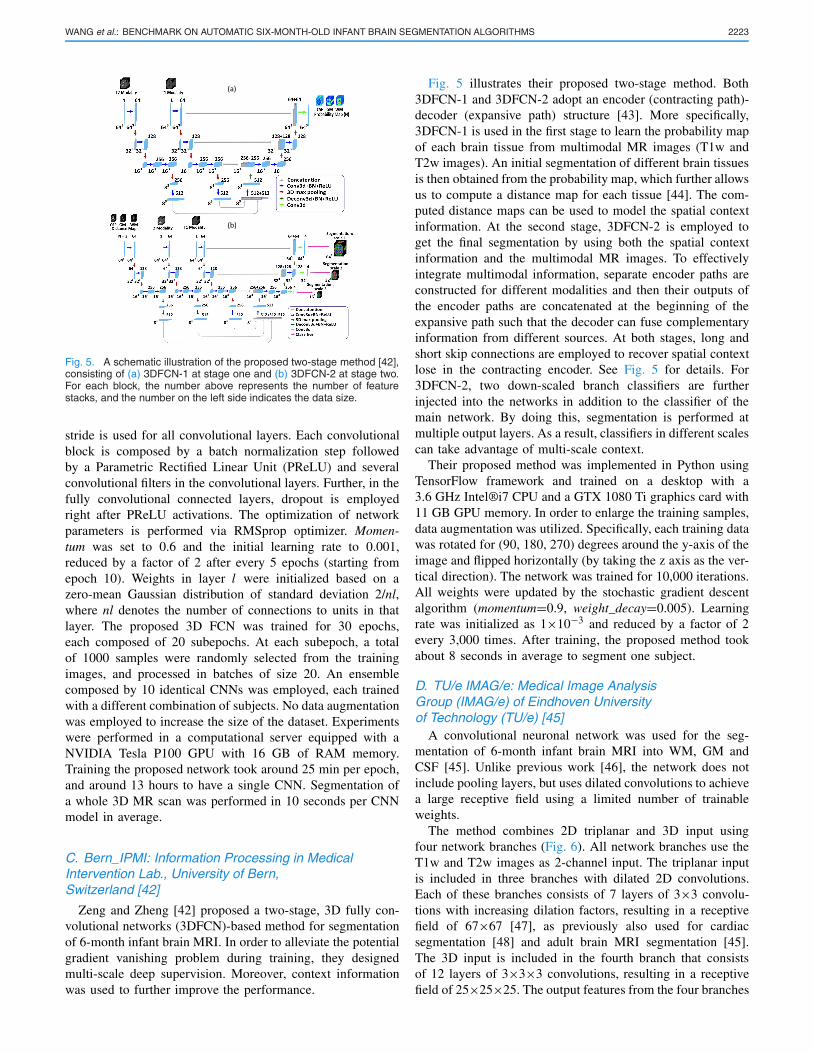
Fig. 5. A schematic illustration of the proposed two-stage method [42],consisting of (a) 3DFCN-1 at stage one and (b) 3DFCN-2 at stage two.For each block, the number above represents the number of featurestacks, and the number on the left side indicates the data size.

stride is used for all convolutional layers. Each convolutionalblock is composed by a batch normalization step followedby a Parametric Rectified Linear Unit (PReLU) and severalconvolutional filters in the convolutional layers. Further, in thefully convolutional connected layers, dropout is employedright after PReLU activations. The optimization of networkparameters is performed via RMSprop optimizer. Momen-tum was set to 0.6 and the initial learning rate to 0.001,reduced by a factor of 2 after every 5 epochs (starting fromepoch 10). Weights in layer l were initialized based on azero-mean Gaussian distribution of standard deviation 2/nl,where nl denotes the number of connections to units in thatlayer. The proposed 3D FCN was trained for 30 epochs,each composed of 20 subepochs. At each subepoch, a totalof 1000 samples were randomly selected from the trainingimages, and processed in batches of size 20. An ensemblecomposed by 10 identical CNNs was employed, each trainedwith a different combination of subjects. No data augmentationwas employed to increase the size of the dataset. Experimentswere performed in a computational server equipped with aNVIDIA Tesla P100 GPU with 16 GB of RAM memory.Training the proposed network took around 25 min per epoch,and around 13 hours to have a single CNN. Segmentation ofa whole 3D MR scan was performed in 10 seconds per CNNmodel in average.

C. Bern_IPMI: Information Processing in MedicalIntervention Lab., University of Bern,Switzerland [42]

Zeng and Zheng [42] proposed a two-stage, 3D fully con-volutional networks (3DFCN)-based method for segmentationof 6-month infant brain MRI. In order to alleviate the potentialgradient vanishing problem during training, they designedmulti-scale deep supervision. Moreover, context informationwas used to further improve the performance.

Fig. 5 illustrates their proposed two-stage method. Both3DFCN-1 and 3DFCN-2 adopt an encoder (contracting path)-decoder (expansive path) structure [43]. More specifically,3DFCN-1 is used in the first stage to learn the probability mapof each brain tissue from multimodal MR images (T1w andT2w images). An initial segmentation of different brain tissuesis then obtained from the probability map, which further allowsus to compute a distance map for each tissue [44]. The com-puted distance maps can be used to model the spatial contextinformation. At the second stage, 3DFCN-2 is employed toget the final segmentation by using both the spatial contextinformation and the multimodal MR images. To effectivelyintegrate multimodal information, separate encoder paths areconstructed for different modalities and then their outputs ofthe encoder paths are concatenated at the beginning of theexpansive path such that the decoder can fuse complementaryinformation from different sources. At both stages, long andshort skip connections are employed to recover spatial contextlose in the contracting encoder. See Fig. 5 for details. For3DFCN-2, two down-scaled branch classifiers are furtherinjected into the networks in addition to the classifier of themain network. By doing this, segmentation is performed atmultiple output layers. As a result, classifiers in different scalescan take advantage of multi-scale context.

Their proposed method was implemented in Python usingTensorFlow framework and trained on a desktop with a3.6 GHz Intel®i7 CPU and a GTX 1080 Ti graphics card with11 GB GPU memory. In order to enlarge the training samples,data augmentation was utilized. Specifically, each training datawas rotated for (90, 180, 270) degrees around the y-axis of theimage and flipped horizontally (by taking the z axis as the ver-tical direction). The network was trained for 10,000 iterations.All weights were updated by the stochastic gradient descentalgorithm (momentum=0.9, weight_decay=0.005). Learningrate was initialized as 1×10−3 and reduced by a factor of 2every 3,000 times. After training, the proposed method tookabout 8 seconds in average to segment one subject.

D. TU/e IMAG/e: Medical Image AnalysisGroup (IMAG/e) of Eindhoven Universityof Technology (TU/e) [45]

A convolutional neuronal network was used for the seg-mentation of 6-month infant brain MRI into WM, GM andCSF [45]. Unlike previous work [46], the network does notinclude pooling layers, but uses dilated convolutions to achievea large receptive field using a limited number of trainableweights.

The method combines 2D triplanar and 3D input usingfour network branches (Fig. 6). All network branches use theT1w and T2w images as 2-channel input. The triplanar inputis included in three branches with dilated 2D convolutions.Each of these branches consists of 7 layers of 3×3 convolu-tions with increasing dilation factors, resulting in a receptivefield of 67×67 [47], as previously also used for cardiacsegmentation [48] and adult brain MRI segmentation [45].The 3D input is included in the fourth branch that consistsof 12 layers of 3×3×3 convolutions, resulting in a receptivefield of 25×25×25. The output features from the four branches


Fig. 6. Network architecture [45]. The colors of the arrows indicate, fromleft to right: 3 × 3 or 3 × 3 × 3 convolutions, concatenation, and 1 × 1convolutions. Dilation factors are shown above the arrows. During thetraining, single voxels are used as output. During the testing, arbitrarilysized outputs can be used, because of the fully convolutional nature ofthe network.

are concatenated and combined in the output layer with1×1 convolutions.

Batch normalization and ReLUs were used throughout.Dropout was used before the output layer. The network wastrained with Adam based on the cross-entropy loss, using mini-batches of 200 or 300 samples in 10 epochs of 50,000 randomsamples per class per training image. The network was trainedwith a patch-based approach, randomly sampling from allimages in the training set. During the testing, arbitrarily sizedinputs can be used, because of the fully convolutional natureof all four branches. The method took about 1 minute tosegment a 3D MRI on a NVIDIA Titan X Pascal GPU.The segmentation results were obtained without any dataaugmentation. Data augmentation could possibly improve theresults in scenarios not well represented in the training set.

E. UPF_Simbiosys: Simbiosys Research Lab atUniversitat Pompeu Fabra (UPF), Barcelona [49]

There exist many segmentation approaches, such as multi-atlas label fusion [50], [51] and learning-based meth-ods [52], [53]. Each method has its own strength, and differentsegmentation approaches may potentially complement eachother. The motivation of the proposed method is to combinethe strengths of complementary methods in a cascaded fashion.

The pipeline of the method is shown in Fig. 7. The 0-levelof the cascade segments the multi-modal (T1w and T2w) inputimages independently with joint label fusion (JLF) [50]. Theestimated probability maps in level-0, along with the originalimages, are inputted to the level-1 of the cascade. In level-1,first, multi-scale features are extracted from both input imagesand probability maps of level-0. Image features consist of1) Gaussian, 2) Laplacian-of-Gaussian, and 3) gradient mag-nitude images convolved with Gaussians at multiple scales foreach modality. Probability features are obtained by convolvingthe level-0 probability maps with Gaussians at multiple scales.

Fig. 7. Dashed blocks correspond to the different levels of the cas-cade [49]. Blue columns denote input, intermediate output, and finalresults. Rounded rectangles denote segmentation methods (orange) andfeature extraction processes (green), respectively.

The multi-scale image and probability-map features are fedinto a SVM classifier for outputting the final estimated labelmap. Each sample of the SVM classifier is composed of thefeatures extracted from each voxel. The SVM classifier istrained during the training phase using the features extractedfrom the training set.

Pre-processing steps include 1) histogram matching of allthe images to the UNC 1-year-old infant template [20], and2) non-rigid registration to the same template using ANTs [54].Pair-wise registrations for multi-atlas JLF are computed byconcatenating registrations through the template. No post-processing steps are applied. The parameters for the seg-mentation methods in each level (i.e., JLF and SVM) arechosen by cross-validation in the training set. Specifically,for JLF, the patch radius is set to be 2 for both modalitiesand the search window is set to be 7 and 5 for T1w and T2wimages, respectively. For SVM, we set the regularization con-stant to C=5, use an RBF kernel, and normalize the featuresto zero-mean and unit standard deviation. The computationaltime for segmenting each subject is ∼30 minutes.

The performance of the SVM classifier in level-1 is highlyinfluenced by the features derived from JLF in level-0. Thissuggests the advantage of combining multiple complementarymethods in the proposed cascaded scheme. A slight drop inperformance is experienced by adding an extra layer in thecascade by the level-1 outputs using as the input, so the two-levels scheme is kept as the final model. Among different com-bination strategies, the proposed cascaded scheme performedbetter than an alternative ensembling strategy [55].

F. NeuroMTL: Montreal Neurological Institute, McGillUniversity, Montreal QC Canada8 [56]

First, an extended training dataset was created by applyingexisting tissue classification to scans from the longitudinaldataset of infants at-risk of autism and control subject inthe Infant Brain Imaging Study (IBIS) [57] where scans of24-month old infants for whom 6 and 12 month scans wereavailable and had T1w and T2w scans acquired at all timepoints (n=216).

8Fonov et al. acknowledged imaging data was collected as part of the InfantBrain Imaging Study (IBIS). Fonov et al. also thank IBIS children and familiesfor their ongoing participation in this longitudinal study.


Fig. 8. Automatic segmentation of 6-month old infant MRI data.

TABLE IPARAMETERS OF 3D U-NET

Tissue classification method is shown in Fig. 8: i) An unbi-ased population average of T1w scans for each age group(6 months, 12 months and 24 months) was created [58].ii) The group average for the 24-month old scans was manuallysegmented into areas of high probability of WM, GM and CSF.iii) All 24-month-old T1w scans were non-linearly registeredto the template, and tissue priors from the template were trans-formed to the space of each subject’s scan. iv) An expectation-maximization algorithm was run to obtain tissue classification.v) Longitudinal non-linear registrations between scans at 6 and12 months and then between 12 and 24 months were per-formed using ANTs with mutual information [54], using bothT1w and T2w scans. Using these registration transformations,tissue classification maps from 24 months were transformedto the 6-month scans. Segmentations from the 24-month scanswere propagated back to the 6-month scans via non-linearregistration. Then, a 3D U-Net [30] was trained in two stageswith the extra dataset to automatically segment healthy tissues.U-Net with 5 downsampling and upsampling blocks with skipconnections was trained on 80×80×80 image patches fortissue classification, with the parameters listed in Table I.Each block contained two convolutional layers with ReLUactivations, with 5×5×5 convolution layers in the first twoblocks, 3×3×3 convolution layers in the next two blocks, anda combination of 3×3×3 and 1×1×1 convolution layers inthe fifth block, with max pooling at each block. Additionally,a 3×3×3 convolution layer with 64 input and output channelswas added, followed by a1×1×1 convolutional layer with64 input and 32 output channels and then another 1×1×1 layerwith 32 input and 4 output channels with dropout, optimizingcategorical cross-entropy with Adam. The output patch wascropped to 64×64×64 to remove edge effects. Training wasdone in two stages, first on the IBIS dataset, and then fine-tuned on the iSeg-2017 challenge data (n=10).

All experiments were performed on a computer with XeonCPU E5-2620 v4 @ 2.10 GHz with 64GB of ram andNVIDIA Titan-X GPU, with deep-net implemented in Torch7.Training on ACE-IBIS dataset took approximately 32 hours(10000 mini-batches), and final training on iSeg-2017 data

Fig. 9. Augmented V-Net. It builds upon the concatenation of theV-Net core network [59] with an augmented path with higher resolution.Augmented V-Net uses a ROI-mask to train only in brain tissue voxels.Layer types are color-coded as shown in the top-right corner.

took 11 hours (4000 mini-batches). Application on a singlesubject, using GPU, took 8 seconds.

G. UPC_DLMI: Signal Theory and CommunicationsDepartment, Universitat Politècnica deCatalunya, Barcelona

Milletari and Ahmadi [59] proposed a convolutional neuralnetwork, named Augmented V-Net (Fig. 9), which is anextension of the V-Net architecture. The main changes withrespect to the original V-Net model can be summarized asfollows:

1) Augmented path: An upsampled version of the input isused to exploit high resolution features. This is doneby upsampling by repetition the input (factor of 2) andstacking several convolutional layers after the upsam-pling. The resultant features are concatenated in the lastlayers.

2) Modified residual connections: The residual connectionsare reformulated such that the propagation of the inputsignal through the network is minimally modified.

3) Mask: A mask is used before the final prediction in orderto constrain the network to train on relevant voxels.

4) Input concatenation: The raw input image is used asfeature map in the last stages of the network.

The key part of the network is the augmented path, whichhas been shown to boost the performance of the standardV-Net for the infant brain segmentation task. It provides high-resolution features by keeping small filter sizes and addingredundancy in the input, helping to detect finer regions suchas boundaries. Later in the network, the authors use the inputimage as raw features, since voxel’s intensities already containvaluable information. Finally, the mask is used to train/predictonly on voxels of brain tissue.

T1w and T2w MRIs are used as input images. Both are nor-malized to zero mean and unit variance. From the normalizedT1w image, a mask is created to mask out background voxels.When training such a big and deep network, there are two mainproblems: GPU memory constraints and the scarcity of data.Patch-wise training arises as a possible solution for the firstissue. The memory required to train Augmented V-Net doesnot allow using dense-training, which is also discouraged whendata is scarce. Larger patch sizes are preferred because theycan encode localization features (brain structures) across thenetwork, while smaller patches allow increasing the batch size


Fig. 10. Visualization of the proposed segmentation network [60].

in the optimization process. The authors finally choose patchesof size 64×64×64 and sample uniformly across the brain,forcing the central voxel to belong to brain tissue (WM, GMand CSF). This size provides the best trade-off between localand contextual information providing faster convergence andlower generalization error.

The authors used data augmentation to increase the size ofthe training set, by making sagittal reflections of each subject.Other reflections have been shown to produce worse results,and no other datasets were used to train the network. In theoptimization process, they used Adam optimizer with initiallearning rate of lr=0.0005. The loss function used was theweighted cross-entropy, where loss weights were computed asthe normalized inverse of the class frequency. At inferencetime, the whole subject can be used as input for the trainedmodel, performing dense inference and using the mask toindicate brain tissue voxels. The method is fully automatic,taking from 5 to 7 seconds to process one subject.

H. LRDE: Epita Research & DevelopmentLaboratory [60]

Xu et al.’s method is an extension from single modalityto multi-modality of the authors’ previous work on neonatalinfant brain MRI segmentation [60]. This automatic methoduses fully convolutional network (FCN) and transfer learning(see details in Fig. 10), and is very fast: the segmentation of awhole volume only takes a few seconds. The core part of the16 layers VGG network [55] is used, which was pre-trained onmillions of 2D color natural images in ImageNet (for imageclassification purpose), and fine-tuned with the MRI trainingdataset. The key contribution is to show how to build 2D colorimages from a 3D MRI volume, so that VGG effectively givesstate-of-the-art segmentation results.

The combination of the T1w and T2w slices to obtaina set of 2D color (RGB) images is very simple. For eachslice (indexed by n), the fake color image is constructed insuch a way that the “green” channel is the T2w slice n, andthe red and the blue are T1w slices respectively at indicesn-1 and n+1. Each 2D color image thus forms a 3D-likerepresentation of a part (3 consecutive slices) of the MRvolume. This representation enables incorporating some 3Dinformation, while avoiding the expensive computational andmemory requirements of fully 3D CNN. For this specificapplication, the fully connected layers at the end of VGGnetwork are discarded; only the 4 stages of convolutional

TABLE IISOURCE CODES FROM TOP-RANKED TEAMS IN ISEG-2017

parts called “base network” are retained. This base networkis composed of convolutional layers, ReLU layers and maxpooling layers between two successive stages. The three maxpooling layers divide the base network into four stages offine to coarse feature maps. A stack of specialized layers isobtained, 1 from each stage, and a softmax function yields thesegmentation result.

Before creating the set of 2D color images, a pre-processingof the T1w and T2w sequences was performed, which con-sists of: 1) shifting the voxel values of the MRI volumesto center their histograms on their maximal histogram value,and 2) requantizing the voxel values on 8 bit (values lowerthan 0 and greater than 255 are saturated). For the training,the classical data augmentation strategy by scaling and rotatingimages were adopted. 2D images were then computed foreach volume of the augmented training base using the pre-processed T1w and T2w slices as described before. Thenetwork was fine-tuned for the first 50K iterations with alearning rate of lr = 10−8, and the last 100K with a smallerlearning rate (lr = 10−10). Stochastic gradient descent wasemployed to minimize the loss function with momentum =0.99 for the first 50K iterations and 0.999 for the next 100k,and weight_decay = 0.0005. The loss function was averagedover 20 images. During test, the runtime on a 3D volumewas 1.8 seconds on average; note that this included the pre-processing step, the computation of the set of 2D color inputimages, and after inference, the reconstruction of a 3D volume(the expected segmentation output) by stacking the set of 2Doutput images.

I. Source CodesA proactive goal of this paper is to encourage authors

to make their codes publicly available for reproducibleresearch. By far, most of teams have shared their codes,as summarized in Table II. For readers who seek to comeup to speed with deep learning, these codes can be alsoserved as good starting points to understand how deep learningalgorithms can be implemented for image segmentation.

V. DISCUSSION

Based on Section IV, 7 out of 8 top-ranked teams adopteddeep learning based algorithms. Moreover, most of the deeplearning related algorithms are based on 3D U-Net (or U-Net-like structures). Thanks to the use of GPUs, most of these


Fig. 11. Performances of the eight top-ranked teams, in terms of DICE,HD95 and ASD, using box-plots. Besides medians, the means are alsoindicated by the dark dots.

algorithms have inference times between 5-10 seconds for awhole MR scan. The only non-deep learning based method isdeveloped by Sanroma et al. (UPF_simbiosys), which employsa multi-atlas based method followed by an SVM to design acascade learning segmentation algorithm.

A. Evaluation in Terms of the Whole BrainWe first evaluate the performance in terms of the whole

brain. Fig. 11 reports performances of the 8 top-ranked teamsin terms of DICE, HD95 and ASD by employing box-plots.Besides medians, the means are also indicated by the blackdiamonds. To know whether any method performs significantlybetter than the others, we calculated Wilcoxon signed-ranktest, as shown in Appendix Table III with all-against-alldiagram in terms of three metrics (DICE, HD95 and ASD).Interestingly, we did not find any method achieving strongstatistically significant better performances compared to allother methods, for segmentation of WM, GM and CSF acrossany metric (DICE, HD95 or ASD). For example, we foundthat the results from MSL_SKKU present the highest medianin terms of DICE for WM. Nevertheless, their differences withthe results obtained by LIVIA and Bern_IPMI are not stronglystatistically significant. In terms of HD95, the results obtainedwith the networks proposed by LRDE and MSL_SKKU havethe lowest median for WM and GM, respectively, but still thereis no strong, statistically significant difference with any othermethods.

B. Evaluation in Terms of ROIsBesides evaluation in terms of the whole brain, we fur-

ther evaluate the performances based on 80 ROIs. Specif-ically, a total of 33 two-year-old subjects were employedas individual atlases (www.brain-development.org) [61]. Eachatlas consists of a T1w MR image and a label imageof 80 ROIs (excluding cerebellum and brainstem). We firstemploy FreeSurfer [62] to segment each T1w MR image intoWM, GM, and CSF. Then, we warp all atlases to each testingsubject’s space based on their tissue segmentation maps usingANTs [63]. Finally, we employ a majority voting to parcellateeach testing subject into 80 ROIs. For each ROI, we employedDICE to measure the performance between automatic segmen-tations and manual segmentation. ROI-based DICE values for

Fig. 12. Error maps: all 8 top-ranked methods produce small errorsin the subcortical regions, but large errors in the cortical regions. Themost error-prone regions are the straight gyrus, lingual gyrus, and medialorbital gyrus. Average error map for all 8 top-ranked methods is shownin the right bottom, with the subcortical mask (caudate nucleus andthalamus). Color bar is from 0 to 1, with the high values indicating largeerrors.

8 top-ranked teams are shown in Appendix Table IV. Due tolarge number of ROIs, p-values for each ROI are not reportedin this paper. However, to better interpret these ROI-basedevaluations, we have generated error maps for each method,as shown in Fig. 12. They were estimated by aligning all theerror maps from 13 testing subjects to a 6-month template [64].The higher value of error map, the higher probability formiss-classification. From all these error maps, we can see allmethods consistently produce small errors in the subcorticalregions, while with larger errors in the cortical regions, whichis actually consistent with the fact that tissue contrast ismuch lower in the cortical regions than subcortical regions.Average error maps for all 8 top-ranked methods were furthergenerated, as shown in the right bottom of Fig. 12. The mosterror-prone ROI regions are the straight gyrus, lingual gyrus,and medial orbital gyrus. These regions are also consistentlyconfirmed with results given in Appendix Table IV, whereDICE values of these ROIs are relatively low, i.e., around 0.84.By contrast, the DICE values of subcortical regions, such asputamen and thalamus, are higher, i.e., around 0.94.

C. Evaluation in Terms of Gyral Landmark CurvesTo better reflect the accuracy of the 8 top-ranked methods,

we further measured the distance of gyral landmark curveson the cortical surfaces. Large curve distance indicates poorperformance on the gyral crest. We selected two major gyri,i.e., the superior temporal gyral curve and the postcentral gyralcurve, as the landmarks to measure the accuracy. We man-ually labeled two sets of gyral curves on the inner corticalsurfaces from different tissue segmentation results [65]. Onetypical example is shown in Fig. 13, in which curves weredelineated by the experts on the superior temporal gyrusand postcentral gyrus: the white curves indicate the groundtruth, and the colored curves indicate results by differentmethods. We employed HD95 to calculate the curve distance,


Fig. 13. Evaluations on gyri for 8 top-ranked methods. The left one showsthe manually labeled postcentral and superior temporal gyral landmarkcurves, used as ground truth; and the right one shows the gyral curvesfrom the segmentation results of 8 top-ranked methods, compared withthe ground truth.

Fig. 14. The boxplot shows HD95 evaluations of 8 top-ranked methodson the superior temporal gyrus and the postcentral gyrus of the 13 testingsubjects. Besides medians, the means are also indicated by the darkdiamonds.

with the median HD95 over 13 testing subjects reported inFig. 14. The p-values were calculated based on Wilcoxonsigned-rank test, as shown in Appendix Table V. We findthat Bern_IPMI achieves the lowest median HD95, but nostatistically significant difference with MSL_SKKU, LIVIA,UPF_simbiosys, and NeuroMTL.

Based on the above evaluations, in terms of the whole brain,small ROIs, and gyral curves, we can observe that none ofthese 8 top-ranked methods has achieved a strong, statisticallysignificant better performance than all other methods. Espe-cially, from the error maps in Fig. 12, these methods con-sistently have a poor performance along the cortical regions.Therefore, there is still opportunity for improvement.

First, all methods directly apply well-established models(e.g., U-Nets) on the challenge, without considering any priorknowledge of infant brain images [66], [67], e.g., corticalthickness is within a certain range. Especially, due to lowcontrast between WM and GM in the 6-month infant brainimages, WM voxels may be under/over segmented. Givena voxel with a resolution of 1×1×1 mm3, although onevoxel error will have a negligible impact on DICE or HD95,it will result in ±1 mm estimation error of cortical thickness.Fig. 15 shows a segmentation result on a testing subjectobtained by MSL_SKKU [31]. Without anatomical guidance,there are many missing gyrus in the reconstructed innersurface by MSL_SKKU [31]. Consequently, the estimatedcortical thickness is abnormally thicker. It is worth noting thatthis type of error should be seriously considered, especiallyfor possible biomarker identification, since this will lead todifficulty of accurately characterizing brain developmental

Fig. 15. Comparison with MSL_SKKU [31] in 2017 MICCAI GrandSegmentation Challenge (iSeg-2017). The results by MSL_SKKU andmanual segmentation are shown in the 1st and 2nd rows, respectively.From left to right: segmentation overlaid on T1w and T2w images, innercortical surface, cortical thickness map, and zoomed views of innercortical surface and cortical thickness map (in mm).

Fig. 16. WM DICE values for each subject by different methods, withthe average DICE represented by the red dashed line.

Fig. 17. The 10th testing subject with motion and unusual scan pose.

attributes, i.e., cortical thickness, gyrification, and convexity.For example, the cortical thickness of the zoomed regions (thelast column of Fig. 15) is abnormally larger than the groundtruth.

Second, all methods ignore a fact that tissue contrastbetween CSF and GM is much higher than that betweenGM and WM. Therefore, it might be reasonable to identifyCSF first from infant brain images to reconstruct the outercortical surface and use it as a guidance to estimate theinner cortical surface, since cortical thickness is within acertain range. Preliminary work on 6-month infant subjectswith risk of autism demonstrates the effectiveness of this kindof strategy [66], [67].

Third, we have inspected the performances of differentmethods for each subject. Fig. 16 shows DICE values foreach subject, with the average DICE represented by the reddashed line. Among all 13 testing subjects, we find that allmethods consistently performed badly on the 2nd and 10th

testing subjects, which were acquired with motion artifacts.Especially, the 10th testing subject presents severe motionartifacts, with one representative slice shown in Fig. 17.Another possible reason could be the different scan pose ofthis subject, compared to other testing subjects. Therefore,the models with robustness to the motion or the scan poseare highly desired, since the motion is inevitable and thesetypes of scan variation are normal during image acquisition.A possible solution to address these issues is to augment the


training images with different rotation degrees, flipping, andsimulated motion artifacts.

Fourth, to better compare these 8 top-ranked methods,Appendix Table VI further lists their key highlights, as well asvarious detailed implementations. For example, all these 8 top-ranked methods randomly selected samples (2D/3D patches)from the training images using moving windows, withoutevaluating the importance of each sample. For example, in theconventional machine learning algorithms, adaptive boostingis an effective strategy to learn features from those error-prone regions to improve the performance [68]. Similarly,the average error map shown in Fig. 12 could potentiallyprovide guidance for selecting effective samples for training.For example, by selecting more training samples from thoseerror-prone regions, the performance of these segmentationalgorithms could be further improved. In addition, fromAppendix Table VI, we can see the patch size used in these8 top-ranked methods varies dramatically from 24×24×24 to80×80×80, which could be further optimized for achievingbetter results.

Finally, we would like to indicate limitations for iSeg-2017.First, we only reviewed the 8 top-ranked teams. Someworks from the remaining teams are also interesting butnot included in this paper, due to space limit. For example,Bernal et al. [69] extended a multi-resolution fully convolu-tional neural to deal with segmentation of 6-month infant brainMRI. Hashemi et al. [70] proposed an exclusive multi-labelmulti-class training strategy to deal with classes that havehighly overlapping features. Second, the number of trainingsubjects and the number of testing subjects are small. Third,image resolution is low, especially for T2w images with1.25×1.25×1.95 mm3 of voxel size. Actually, in the currentBCP imaging protocol [3], T1w and T2w images are acquiredwith 0.8×0.8×0.8 mm3. These limitations will be alleviated,such as by including subjects acquired in BCP, for our planned2019 iSeg Grand Challenge (https://iseg2019.web.unc.edu).

VI. CONCLUSION

In this paper, we have reviewed and summarized 21 auto-matic segmentation methods participating in iSeg-2017. Espe-cially, we have elaborated the details of 8 top-ranked methods:including the pipeline, implementation, and source code.We further pointed out limitations and possible future direc-tions. The iSeg-2017 website is always open and we hopeour manual labels in iSeg-2017, this review article and sourcecodes could greatly advance methodological development inthe community.

REFERENCES

[1] G. Li et al., “Mapping region-specific longitudinal cortical surfaceexpansion from birth to 2 years of age,” Cerebral Cortex, vol. 23,pp. 2724–2733, Nov. 2013.

[2] G. Li et al., “Mapping longitudinal hemispheric structural asymmetriesof the human cerebral cortex from birth to 2 years of age,” CerebralCortex, vol. 24, no. 5, pp. 1289–1300, May 2014.

[3] B. R. Howell et al., “The UNC/UMN Baby Connectome Project(BCP): An overview of the study design and protocol development,”NeuroImage, vol. 185, pp. 891–905, Jan. 2019.

[4] G. Li et al., “Early diagnosis of autism disease by multi-channel CNNs,”in Machine Learning in Medical Imaging. Cham, Switzerland: Springer,2018, pp. 303–309.

[5] L. Wang et al., “Segmentation of neonatal brain MR images using patch-driven level sets,” NeuroImage, vol. 84, pp. 141–158, Jan. 2014.

[6] L. Wang et al., “LINKS: Learning-based multi-source IntegratioNframeworK for Segmentation of infant brain images,” NeuroImage,vol. 108, pp. 72–160, Mar. 2015.

[7] S. Hu et al., “Learning-based deformable image registration for infantMR images in the first year of life,” Med. Phys., vol. 44, no. 1,pp. 158–170, Jan. 2017.

[8] F. Shi et al., “Neonatal atlas construction using sparse representation,”Hum. Brain Mapping, vol. 35, no. 9, pp. 4663–4677, Sep. 2014.

[9] F. Shi et al., “Construction of multi-region-multi-reference atlasesfor neonatal brain MRI segmentation,” NeuroImage, vol. 51, no. 2,pp. 684–693, Jun. 2010.

[10] T. Paus, D. L. Collins, A. C. Evans, G. Leonard, B. Pike, andA. Zijdenbos, “Maturation of white matter in the human brain: A reviewof magnetic resonance studies,” Brain Res. Bull., vol. 54, pp. 255–266,Feb. 2001.

[11] Z. Xue, D. Shen, and C. Davatzikos, “CLASSIC: Consistent longitudinalalignment and segmentation for serial image computing,” NeuroImage,vol. 30, no. 2, pp. 388–399, Apr. 2006.

[12] G. Li et al., “Computational neuroanatomy of baby brains: A review,”NeuroImage, vol. 185, pp. 906–925, Jan. 2018.

[13] I. Išgum et al., “Evaluation of automatic neonatal brain segmentationalgorithms: The NeoBrainS12 challenge,” Med. Image Anal., vol. 20,no. 1, pp. 135–151, Feb. 2015.

[14] A. M. Mendrik et al., “MRBrainS challenge: Online evaluation frame-work for brain image segmentation in 3T MRI scans,” Comput. Intell.Neurosci., vol. 2015, Jan. 2015, pp. 1–16.

[15] S. Winzeck et al., “Isles 2016 and 2017-benchmarking ischemic strokelesion outcome prediction based on multispectral MRI,” Frontiers Neu-rol., vol. 9, p. 679, Sep. 2018.

[16] B. H. Menze et al., “The multimodal brain tumor image segmenta-tion benchmark (BRATS),” IEEE Trans. Med. Imag., vol. 34, no. 10,pp. 1993–2024, Oct. 2015.

[17] W. Zhang et al., “Deep convolutional neural networks for multi-modalityisointense infant brain image segmentation,” NeuroImage, vol. 108,pp. 214–224, Mar. 2015.

[18] L. Wang et al., “Integration of sparse multi-modality representation andanatomical constraint for isointense infant brain MR image segmenta-tion,” NeuroImage, vol. 89, pp. 64–152, Apr. 2014.

[19] D. Nie, L. Wang, E. Adeli, C. Lao, W. Lin, D. Shen, “3-D fullyconvolutional networks for multimodal isointense infant brain imagesegmentation,” IEEE Trans. Cybern., vol. 49, no. 3, pp. 1123–1136,Mar. 2019.

[20] F. Shi, L. Wang, Y. Dai, J. H. Gilmore, W. Lin, and D. Shen, “LABEL:Pediatric brain extraction using learning-based meta-algorithm,” Neu-roImage, vol. 62, no. 3, pp. 1975–1986, 2012.

[21] J. G. Sled, A. P. Zijdenbos, and A. C. Evans, “A nonparametric methodfor automatic correction of intensity nonuniformity in MRI data,” IEEETrans. Med. Imag., vol. 17, no. 1, pp. 87–97, Feb. 1998.

[22] L. Wang, F. Shi, P.-T. Yap, W. Lin, J. H. Gilmore, and D. Shen,“Longitudinally guided level sets for consistent tissue segmentation ofneonates,” Hum. Brain Mapping, vol. 34, no. 4, pp. 956–972, Apr. 2013.

[23] Y. Dai, F. Shi, L. Wang, G. Wu, and D. Shen, “iBEAT: A toolbox forinfant brain magnetic resonance image processing,” Neuroinformatics,vol. 11, no. 2, pp. 211–225 , Apr. 2013.

[24] J. G. Chi, E. C. Dooling, and F. H. Gilles, “Gyral development of thehuman brain,” Ann. Neurol., vol. 1, no. 1, pp. 86–93, Jan. 1977.

[25] E. Armstrong, A. Schleicher, H. Omran, M. Curtis, and K. Zilles,“The ontogeny of human gyrification,” Cerebral Cortex, vol. 5,pp. 56–63, Jan./Feb. 1995.

[26] J. Hill et al., “A surface-based analysis of hemispheric asymmetries andfolding of cerebral cortex in term-born human infants,” J. Neurosci.,vol. 30, pp. 2268–2276, Feb. 2010.

[27] J. Dubois et al., “Mapping the early cortical folding process in thepreterm newborn brain,” Cerebral Cortex, vol. 18, pp. 1444–1454,Jun. 2008.

[28] S. Abe, K. Takagi, T. Yamamoto, Y. Okuhata, and T. Kato, “Assessmentof cortical gyrus and sulcus formation using MR images in normalfetuses,” Prenatal Diagnosis, vol. 23, no. 3, pp. 225–231, Mar. 2003.

[29] C. Lebel, L. Walker, A. Leemans, L. Phillips, and C. Beaulieu,“Microstructural maturation of the human brain from childhood toadulthood,” NeuroImage, vol. 40, no. 3, pp. 1044–1055, Apr. 2008.


[30] Ö. Çiçek, A. Abdulkadir, S. S. Lienkamp, T. Brox, and O. Ronneberger,“3D U-Net: Learning dense volumetric segmentation from sparse anno-tation,” in Proc. MICCAI, 2016, pp. 424–432.

[31] T. D. Bui, J. Shin, and T. Moon. (2017). “3D densely convolu-tional networks for volumetric segmentation.” [Online]. Available:https://arxiv.org/abs/1709.03199

[32] G. Huang, Z. Liu, L. van der Maaten, and K. Q. Weinberger,“Densely connected convolutional networks,” in Proc. CVPR, Jun. 2017,pp. 2261–2269.

[33] S. Ioffe and C. Szegedy. (2015). “Batch normalization: Acceleratingdeep network training by reducing internal covariate shift.” [Online].Available: https://arxiv.org/abs/1502.03167

[34] X. Glorot, A. Bordes, and Y. Bengio, “Deep Sparse Rectifier Neural Net-works,” in Proc. 14th Int. Conf. Artif. Intell. Statist., 2011, pp. 315–323.

[35] N. Srivastava, G. Hinton, A. Krizhevsky, I. Sutskever, andR. Salakhutdinov, “Dropout: A simple way to prevent neural networksfrom overfitting,” J. Mach. Learn. Res., vol. 15, no. 1, pp. 1929–1958,2014.

[36] J. Long, E. Shelhamer, and T. Darrell, “Fully convolutional networksfor semantic segmentation,” in Proc. CVPR, Jun. 2015, pp. 3431–3440.

[37] D. P. Kingma and J. Ba. (2017). “Adam: A method for stochasticoptimization.” [Online]. Available: https://arxiv.org/abs/1412.6980

[38] K. He, X. Zhang, S. Ren, and J. Sun, “Delving deep into rectifiers: Sur-passing human-level performance on imagenet classification,” in Proc.ICCV, 2015, pp. 1026–1034.

[39] Y. Jia et al., “Caffe: Convolutional architecture for fast feature embed-ding,” in Proc. 22nd ACM Int. Conf. Multimedia, 2014, pp. 675–678.

[40] J. Dolz, C. Desrosiers, L. Wang, J. Yuan, D. Shen, andI. Ben Ayed. (2017). “Deep CNN ensembles and suggestive anno-tations for infant brain MRI segmentation.” [Online]. Available:https://arxiv.org/abs/1712.05319

[41] J. Dolz, C. Desrosiers, and I. B. Ayed, “3D fully convolutional networksfor subcortical segmentation in MRI: A large-scale study,” NeuroImage,vol. 170, pp. 456–470, Apr. 2018.

[42] G. Zeng and G. Zheng, “Multi-stream 3D FCN with multi-scale deepsupervision for multi-modality isointense infant brain MR image seg-mentation,” in Proc. ISBI, Apr. 2018, pp. 136–140.

[43] O. Ronneberger, P. Fischer, and T. Brox, “U-Net: Convolutional Net-works for Biomedical Image Segmentation,” in Proc. MICCAI, 2015,pp. 234–241.

[44] R. Kimmel, N. Kiryati, and A. M. Bruckstein, “Sub-pixel distance mapsand weighted distance transforms,” J. Math. Imag. Vis., vol. 6, nos. 2–3,pp. 223–233, Jun. 1996.

[45] P. Moeskops and J. P. W. Pluim. (2017). “Isointense infant brain MRIsegmentation with a dilated convolutional neural network.” [Online].Available: https://arxiv.org/abs/1708.02757

[46] P. Moeskops, M. A. Viergever, A. M. Mendrik, L. S. de Vries,M. J. N. L. Benders, and I. Išgum, “Automatic segmentation of MRbrain images with a convolutional neural network,” IEEE Trans. Med.Imag., vol. 35, no. 5, pp. 1252–1261, May 2016.

[47] F. Yu and V. Koltun. (2015). “Multi-scale context aggregation by dilatedconvolutions.” [Online]. Available: https://arxiv.org/abs/1511.07122

[48] J. M. Wolterink, T. Leiner, M. A. Viergever, and I. Išgum, “Dilatedconvolutional neural networks for cardiovascular MR segmentationin congenital heart disease,” in Reconstruction, Segmentation, andAnalysis of Medical Images. Cham, Switzerland: Springer, 2016,pp. 95–102.

[49] G. Sanroma, O. M. Benkarim, G. Piella, and M. A. G. Ballester,“Building an ensemble of complementary segmentation methods byexploiting probabilistic estimates,” in Machine Learning in MedicalImaging. Cham, Switzerland: Springer, 2016, pp. 27–35.

[50] H. Wang, J. W. Suh, S. R. Das, J. B. Pluta, C. Craige, andP. A. Yushkevich, “Multi-atlas segmentation with joint label fusion,”IEEE Trans. Pattern Anal. Mach. Intell., vol. 35, no. 3, pp. 611–623,Mar. 2013.

[51] G. Wu, Q. Wang, D. Zhang, F. Nie, H. Huang, and D. Shen,“A generative probability model of joint label fusion for multi-atlas based brain segmentation,” Med. Image Anal., vol. 18, no. 6,pp. 881–890, 2014.

[52] Y. Hao et al., “Local label learning (LLL) for subcortical structuresegmentation: Application to hippocampus segmentation,” Hum. BrainMapping, vol. 35, no. 6, pp. 2674–2697, Jun. 2014.

[53] P. Moeskops et al., “Automatic segmentation of MR brain images ofpreterm infants using supervised classification,” NeuroImage, vol. 118,pp. 628–641, Sep. 2015.

[54] B. B. Avants, N. J. Tustison, G. Song, P. A. Cook, A. Klein, andJ. C. Gee, “A reproducible evaluation of ANTs similarity metric per-formance in brain image registration,” NeuroImage, vol. 54, no. 3,pp. 2033–2044, Feb. 2011.

[55] K. Simonyan and A. Zisserman. (2015). “Very deep convolutionalnetworks for large-scale image recognition.” [Online]. Available:https://arxiv.org/abs/1409.1556

[56] V. Fonov, A. Doyle, A. C. Evans, and L. Collins. (2018).NeuroMTL iSEG Challenge Methods. [Online]. Available:https://www.biorxiv.org/content/10.1101/278465v1

[57] H. C. Hazlett, H. Gu, and The IBIS Network, “Early brain developmentin infants at high risk for autism spectrum disorder,” Nature, vol. 542,pp. 348–351, Feb. 2017.

[58] V. Fonov, A. C. Evans, K. Botteron, C. R. Almli, R. C. McKinstry, andD. L. Collins, “Unbiased average age-appropriate atlases for pediatricstudies,” NeuroImage, vol. 54, no. 1, pp. 313–327, Jan. 2011.

[59] F. Milletari, N. Navab, and S.-A. Ahmadi. (2016). “V-Net: Fully convo-lutional neural networks for volumetric medical image segmentation.”[Online]. Available: https://arxiv.org/abs/1606.04797

[60] Y. Xu, T. Géraud, and I. Bloch, “From neonatal to adult brain MR imagesegmentation in a few seconds using 3D-like fully convolutional networkand transfer learning,” in Proc. ICIP, Sep. 2017, pp. 4417–4421.

[61] I. S. Gousias et al., “Automatic segmentation of brain MRIs of 2-year-olds into 83 regions of interest,” NeuroImage, vol. 40, pp. 672–684,Apr. 2008.

[62] B. Fischl, “FreeSurfer,” NeuroImage, vol. 62, pp. 774–781, Aug. 2012.[63] B. B. Avants, C. L. Epstein, M. Grossman, and J. C. Gee, “Symmet-

ric diffeomorphic image registration with cross-correlation: Evaluatingautomated labeling of elderly and neurodegenerative brain,” Med. ImageAnal., vol. 12, no. 1, pp. 26–41, Feb. 2008.

[64] Y. Zhang, F. Shi, G. Wu, L. Wang, P.-T. Yap, and D. Shen, “Consistentspatial-temporal longitudinal atlas construction for developing infantbrains,” IEEE Trans. Med. Imag., vol. 35, no. 12, pp. 2568–2577,Dec. 2016.

[65] G. Li, L. Guo, J. Nie, and T. Liu, “An automated pipeline for corti-cal sulcal fundi extraction,” Med. Image Anal., vol. 14, pp. 343–359,Jun. 2010.

[66] L. Wang et al., “Volume-based analysis of 6-month-old infant brainMRI for autism biomarker identification and early diagnosis,” in Proc.MICCAI, 2018, pp. 411–419.

[67] L. Wang et al., “Anatomy-guided joint tissue segmentation and topolog-ical correction for 6-month infant brain MRI with risk of autism,” Hum.Brain Mapping, vol. 39, no. 6, pp. 2609–2623, Jun. 2018.

[68] S. Shalev-Shwartz. (2017). “SelfieBoost: A boosting algorithm for deeplearning.” [Online]. Available: https://arxiv.org/abs/1411.3436

[69] J. Bernal, K. Kushibar, M. Cabezas, S. Valverde, A. Oliver, andX. Lladó. (2018). “Quantitative analysis of patch-based fully con-volutional neural networks for tissue segmentation on brain mag-netic resonance imaging.” [Online]. Available: https://arxiv.org/abs/1801.06457

[70] S. R. Hashemi, S. P. Prabhu, S. K. Warfield, and A. Gholipour,“Exclusive independent probability estimation using deep 3D fullyconvolutional DenseNets: Application to IsoIntense infant brain MRIsegmentation,” in Proc. 2nd Int. Conf. Med. Imag. Deep Learn., 2019,pp. 1–14.

Documents

Benchmark on Automatic Six-Month-Old Infant Brain